Jittering and Clustering:Strategies for the Construction of Robust Designs

Abstract

We first discuss, and give examples of, methods for randomly implementing some minimax robust designs from the literature. These have the advantage, over their deterministic counterparts, of having bounded maximum loss in large and very rich neighbourhoods of the, almost certainly inexact, response model fitted by the experimenter. Their maximum loss rivals that of the theoretically best possible, but not implementable, minimax design. The procedures are then extended to more general robust designs. For two-dimensional designs we sample from contractions of Voronoi tessellations, generated by selected basis points, which partition the design space. These ideas are then extended to $k$-dimensional designs for general $k$.

1 Introduction and summary

In this article we investigate various methods of implementing experimental designs, robust against model inadequacies. We begin with a review of the ‘minimax’ theory of robustness of design, and of some minimax designs from the literature. It will be seen that the designs which protect against a large class of alternative response models are necessarily absolutely continuous, and so lose their optimality when approximated by implementable, discrete (deterministic) designs. Two remedies for this and other issues are proposed, suggested by work of Waite and Woods (2022), who propose and study random design strategies.

The first remedy is a random design strategy termed jittering. The designs are obtained by uniform sampling from small neighbourhoods of an optimal set $t^{\ast}=\left\{t_{i}|i=1,...,n\right\}$ of points, chosen to approximate the minimax design density. Both completely random and stratified random – i.e. random within each neighbourhood – are considered. We assess these designs by looking at the sample distributions of the mean squared prediction errors incurred; with respect to these measures both sampling strategies typically lead to designs very nearly optimal, with the stratification strategy clearly outperforming its completely random counterpart.

We then investigate a strategy leading to cluster designs, motivated by the observation that robust designs for a particular response model tend to place their mass near those points $t_{i}$ at which classically optimal designs, focussed solely on variance minimization, are replicated – but with their support points spread out in clusters of nearby points, rather than being replicated. In clustering the idea is to sample from densities concentrated near the $t_{i}$. An advantage to this method over jittering is that there is no need for the minimax design to already have been derived.

Both these approaches parallel the ‘random translation design strategy’ of Waite and Woods (2022), who sample uniformly in small neighbourhoods of a chosen set of points, but with some significant differences. The choice of $t^{\ast}$ in jittering allows for designs whose maximum expected loss rivals that of the minimax, absolutely continuous design. In clustering, both the support of the non-uniform densities from which we sample, and the extent of their concentration near the $t_{i}$, are governed by a user-chosen parameter $\nu$, representing the bias/variance trade-off desired by a user seeking robustness against model misspecifications.

We start by applying these ideas in several one-dimensional cases for which the minimax designs have been derived. We then consider two-dimensional applications in which intervals containing the $t_{i}$ are replaced by less regular regions formed by shrinking Voronoi tessellations generated by $t^{\ast}$. We finish with recommendations for the construction of $k$-dimensional designs for $k\geq 3$. The examples were prepared using matlab; the code is available on the author’s website.

2 Minimax robustness of design

The theory of robustness of design was largely initiated by Box and Draper (1959), who investigated the robustness of some classical experimental designs in the presence of certain model inadequacies, e.g. designs optimal for a low order polynomial response when the true response was a polynomial of higher order. Huber (1975) derived minimax designs for straight line regression; these minimize the maximum integrated mean squared error, with the maximum taken over a large class of alternative responses. Wiens (1990, 1992) extended these results to multiple regression responses and in a variety of other directions – see Wiens (2015) for a summary of these and other approached to robustness of design. Specifically, the general problem is phrased in terms of an approximate regression response

$$E\left[Y\left(\boldsymbol{x}\right)\right]\approx\boldsymbol{f}^{\prime}\left(\boldsymbol{x}\right)\boldsymbol{\theta},$$ (1)

for $p$ regressors $\boldsymbol{f}$, each functions of $q$ independent variables $\boldsymbol{x}$, and a parameter $\boldsymbol{\theta}$. Since (1) is an approximation the interpretation of $\boldsymbol{\theta}$ is unclear; we define this target parameter by

$$\boldsymbol{\theta}=\arg\min_{\boldsymbol{\eta}}\int_{\mathcal{X}}\left(E\left[Y\left(\boldsymbol{x}\right)\right]-\boldsymbol{f}^{\prime}\left(\boldsymbol{x}\right)\boldsymbol{\eta}\right)^{2}\mu\left(d\boldsymbol{x}\right),$$ (2)

where $\mu\left(d\boldsymbol{x}\right)$ represents either Lebesgue measure or counting measure, depending upon the nature of the design space $\mathcal{X}$. We then define $\psi\left(\boldsymbol{x}\right)=E\left[Y\left(\boldsymbol{x}\right)\right]-\boldsymbol{f}^{\prime}\left(\boldsymbol{x}\right)\boldsymbol{\theta}$. This results in the class of responses $E\left[Y\left(\boldsymbol{x}\right)\right]=\boldsymbol{f}^{\prime}\left(\boldsymbol{x}\right)\boldsymbol{\theta}+\psi\left(\boldsymbol{x}\right)$, with – by virtue of (2) – $\psi$ satisfying the orthogonality requirement

$$\int_{\mathcal{X}}\boldsymbol{f}\left(\boldsymbol{x}\right)\psi\left(\boldsymbol{x}\right)\mu\left(d\boldsymbol{x}\right)=\boldsymbol{0}.\$$ (3)

Assuming that $\mathcal{X}$ is large enough that the matrix $\boldsymbol{A}=\int_{\mathcal{X}}\boldsymbol{f}\left(\boldsymbol{x}\right)\boldsymbol{f}^{\prime}\left(\boldsymbol{x}\right)\mu\left(d\boldsymbol{x}\right)$ is invertible, the parameter defined by (2) and (3) is unique.

We identify a design with its design measure – a probability measure $\xi\left(d\boldsymbol{x}\right)$ on $\mathcal{X}$. Define

$$\boldsymbol{M}_{\xi}=\int_{\mathcal{X}}\boldsymbol{f}\left(\boldsymbol{x}\right)\boldsymbol{f}^{\prime}\left(\boldsymbol{x}\right)\xi\left(d\boldsymbol{x}\right),\text{ \ }\boldsymbol{b}_{\psi,\xi}=\int_{\mathcal{X}}\boldsymbol{f}\left(\boldsymbol{x}\right)\psi\left(\boldsymbol{x}\right)\xi\left(d\boldsymbol{x}\right),$$

and assume $\xi$ is such that $\boldsymbol{M}_{\xi}$ is invertible. The covariance matrix of the least squares estimator $\boldsymbol{\hat{\theta}}$, assuming homoscedastic errors with variance $\sigma_{\varepsilon}^{2}$, is $\left(\sigma_{\varepsilon}^{2}/n\right)\boldsymbol{M}_{\xi}^{-1}$, and the bias is $E\left[\boldsymbol{\hat{\theta}}-\boldsymbol{\theta}\right]=\boldsymbol{M}_{\xi}^{-1}\boldsymbol{b}_{\psi,\xi}$; together these yield the mean squared error (mse) matrix

$$\text{{mse}}\left[\boldsymbol{\hat{\theta}}\right]=\frac{\sigma_{\varepsilon}^{2}}{n}\boldsymbol{M}_{\xi}^{-1}+\boldsymbol{M}_{\xi}^{-1}\boldsymbol{b}_{\psi,\xi}\boldsymbol{b}_{\psi,\xi}^{\prime}\boldsymbol{M}_{\xi}^{-1}$$

of the parameter estimates, whence the mse of the fitted values $\hat{Y}\left(\boldsymbol{x}\right)=\boldsymbol{f}^{\prime}\left(\boldsymbol{x}\right)\boldsymbol{\hat{\theta}}$ is

$$\text{{mse}}\left[\hat{Y}\left(\boldsymbol{x}\right)\right]=\frac{\sigma_{\varepsilon}^{2}}{n}\boldsymbol{f}^{\prime}\left(\boldsymbol{x}\right)\boldsymbol{M}_{\xi}^{-1}\boldsymbol{f}\left(\boldsymbol{x}\right)+\left(\boldsymbol{f}^{\prime}\left(\boldsymbol{x}\right)\boldsymbol{M}_{\xi}^{-1}\boldsymbol{b}_{\psi,\xi}\right)^{2}.$$

A loss function that is commonly employed is the integrated mse of the predictions:

$$\text{{imse}}\left(\xi|\psi\right)=\int_{\mathcal{X}}\text{{mse}}\left[\hat{Y}\left(\boldsymbol{x}\right)\right]d\boldsymbol{x}=\frac{\sigma_{\varepsilon}^{2}}{n}tr\left(\boldsymbol{AM}_{\xi}^{-1}\right)+\boldsymbol{b}_{\psi,\xi}^{\boldsymbol{\prime}}\boldsymbol{M}_{\xi}^{-1}\boldsymbol{AM}_{\xi}^{-1}\boldsymbol{b}_{\psi,\xi}+\int_{\mathcal{X}}\psi^{2}\left(\boldsymbol{x}\right)\mu\left(d\boldsymbol{x}\right)\mathbf{.}$$ (4)

The dependence on $\psi$ is eliminated by adopting a minimax approach, according to which one first maximizes (4) over a neighbourhood of the assumed response. This neighbourhood is constrained by (3) and by a bound $\int_{\mathcal{X}}\psi^{2}\left(\boldsymbol{x}\right)\mu\left(d\boldsymbol{x}\right)\leq\tau^{2}/n$, required so that errors due to bias and to variation remain of the same order, asymptotically.

Huber (1975) took $\mathcal{X}$ to be an interval of the real line and assumed that the minimax design measure had a density $m\left(x\right)$; Wiens (1992) justified this assumption by proving that any design whose design space $\mathcal{X}$ has positive Lebesgue measure, and which places positive mass on a set of Lebesque measure zero, necessarily has $\sup_{\psi}$imse$\left(\xi|\psi\right)=\infty$. Thus in order that a design on an interval, hypercube, etc. have finite maximum loss, it must be absolutely continuous. For such a design $\max_{\psi}$imse$\left(\xi|\psi\right)$ is $\left(\sigma_{\varepsilon}^{2}+\tau^{2}\right)/n$ times

$$I_{\nu}\left(\xi\right)=\left(1-\nu\right)tr\boldsymbol{AM}_{\xi}^{-1}+\nu ch_{\max}\boldsymbol{K}_{\xi}\boldsymbol{H}_{\xi}^{-1},$$ (5)

where

$$\boldsymbol{H}\mathbf{{}_{\xi}}=\boldsymbol{M}\mathbf{{}_{\xi}}\boldsymbol{A}^{-1}\boldsymbol{M}_{\xi},\text{ }\boldsymbol{K}_{\xi}=\int_{\mathcal{X}}\boldsymbol{f}\left(\boldsymbol{x}\right)\boldsymbol{f}^{\prime}\left(\boldsymbol{x}\right)m^{2}\left(\boldsymbol{x}\right)d\boldsymbol{x},$$

$ch_{\max}$ denotes the maximum eigenvalue and $\nu=\tau^{2}\left/\left(\sigma_{\varepsilon}^{2}+\tau^{2}\right)\right.\in\left[0,1\right]$, representing the relative importance, to the experimenter, of errors due to bias rather than to variance. With

$$\boldsymbol{G}_{\xi} = \boldsymbol{K}_{\xi}-\boldsymbol{H}_{\xi}=\int_{\mathcal{X}}\left[\left(m\left(\boldsymbol{x}\right)\boldsymbol{I}_{p}-\boldsymbol{M}_{\xi}\boldsymbol{A}^{-1}\right)\boldsymbol{f}\left(\boldsymbol{x}\right)\right]\left[\left(m\left(\boldsymbol{x}\right)\boldsymbol{I}_{p}-\boldsymbol{M}_{\xi}\boldsymbol{A}^{-1}\right)\boldsymbol{f}\left(\boldsymbol{x}\right)\right]^{\boldsymbol{\prime}}d\boldsymbol{x}\mathbf{,}$$

$$\mathbf{r}_{\xi}\left(\boldsymbol{x}\right) = \frac{\tau}{\sqrt{n}}\boldsymbol{G}_{\xi}^{-1/2}\left(m\left(\boldsymbol{x}\right)\boldsymbol{I}_{p}-\boldsymbol{M}_{\xi}\boldsymbol{A}^{-1}\right)\boldsymbol{f}\left(\boldsymbol{x}\right),$$ (6)

the least favourable contaminant is

$$\psi_{\xi}\left(\boldsymbol{x}\right)=\mathbf{r}_{\xi}^{\prime}\left(\boldsymbol{x}\right)\mathbf{\beta_{\xi},\ }$$ (7)

where $\mathbf{\beta}_{\xi}$ is the unit eigenvector belonging to the maximum eigenvalue of $\boldsymbol{G}_{\xi}^{1/2}\boldsymbol{H}_{\xi}^{-1}\boldsymbol{G}_{\xi}^{1/2}+\boldsymbol{I}_{p}$. See Wiens (2015) for details and further references.

2.1 Random designs

In the following sections we construct distributions $\Phi\left(\boldsymbol{x}\right)$, with densities $\phi\left(\boldsymbol{x}\right)$, and propose randomly choosing design points from $\Phi$. An $n$-point design $D=\left\{\boldsymbol{x}_{i}\right\}_{i=1}^{n}$ chosen in this way has design measure $\delta=n^{-1}\sum\delta_{\boldsymbol{x}_{i}}$, where $\delta_{\boldsymbol{x}_{i}}$ is point mass at $\boldsymbol{x}_{i}\sim\Phi$. By the preceding any such design has unbounded imse once it is chosen. Of interest however is the expected imse against a common alternative; for this we evaluate at the least favourable contaminant $\psi_{\Phi}$, given by (6) and (7) but with $\xi$ replaced by $\Phi$. It is shown in the Appendix that

$$E_{\Phi}\left[\text{{imse}}\left(\delta|\psi_{\Phi}\right)\right]=\left(\sigma_{\varepsilon}^{2}+\tau^{2}\right)/n\times J_{\nu}\left(\Phi\right),$$ (8)

where

$$J_{\nu}\left(\Phi\right) = \left(1-\nu\right)E_{\Phi}\left[tr\boldsymbol{AM}_{\delta}^{-1}\right]+\nu E_{\Phi}\left[\gamma_{\delta}\right]\text{, for}$$ (9)

$$\gamma_{\delta} = \mathbf{\beta}_{\Phi}^{\prime}\boldsymbol{G}_{\Phi}^{-1/2}\left(\boldsymbol{M}_{\phi}\boldsymbol{M}_{\delta}^{-1}-\boldsymbol{M}_{\Phi}\boldsymbol{A}^{-1}\right)\boldsymbol{A}\left(\boldsymbol{M}_{\delta}^{-1}\boldsymbol{M}_{\phi}-\boldsymbol{A}^{-1}\leavevmode\nobreak\ \boldsymbol{M}_{\Phi}\right)\boldsymbol{G}_{\Phi}^{-1/2}\mathbf{\beta}_{\Phi}+1\text{.}$$

Here $\boldsymbol{M}_{\delta}\overset{def}{=}\frac{1}{n}\sum_{\boldsymbol{x}_{i}\in D}\boldsymbol{f}\left(\boldsymbol{x}_{i}\right)\boldsymbol{f}^{\prime}\left(\boldsymbol{x}_{i}\right)$ and $\boldsymbol{M}_{\phi}\overset{def}{=}\frac{1}{n}\sum_{\boldsymbol{x}_{i}\in D}\boldsymbol{f}\left(\boldsymbol{x}_{i}\right)\phi\left(\boldsymbol{x}_{i}\right)\boldsymbol{f}^{\prime}\left(\boldsymbol{x}_{i}\right)$; $\mathbf{\beta}_{\Phi}$ is the unit eigenvector belonging to the maximum eigenvalue of $\boldsymbol{G}_{\Phi}^{1/2}\boldsymbol{H}_{\Phi}^{-1}\boldsymbol{G}_{\Phi}^{1/2}+\boldsymbol{I}_{p}$.

Note that both $\boldsymbol{M}_{\delta}$ and $\boldsymbol{M}_{\phi}$ are random. The expectations in (9) can be estimated by averaging over a large number of realizations of $\delta$ – see §4.1 for an example of this.

In the special case that $\phi\left(\boldsymbol{x}\right)$ is constant on its support – as is the case in §3 – $\boldsymbol{M}_{\delta}^{-1}\boldsymbol{M}_{\phi}$ is a constant multiple of $\boldsymbol{I}_{p}$, $\gamma_{\delta}$ is non-random, and these formulas simplify considerably – see (12).

3 Jittering

There are obvious issues in implementing an absolutely continuous design measure within this framework, since any discrete approximation necessarily suffers from the drawback, as above, that the maximum loss is infinite. Noting that in this case the least favourable contaminating function $\psi$ is largely concentrated on a set of measure zero – an unlikely eventuality against which to seek protection – Wiens (1992, p. 355) states that “Our attitude is that an approximation to a design which is robust against more realistic alternatives is preferable to an exact solution in a neighbourhood which is unrealistically sparse.” He places one observation at each of the quantiles

$$t_{i}=\xi^{-1}\left(\frac{i-1/2}{n}\right),\ i=1,...,n,$$ (10)

which is the $n$-point design closest to $\xi$ in Kolmogorov distance (Fang and Wang 1994; see Xu and Yuen 2011 for other possibilities).

Despite the disclaimer above, such discrete implementations have become controversial; see in particular Bischoff (2010). In this article we investigate a resolution to these difficulties offered by Waite and Woods (2022), who propose randomly sampling the design points from uniform densities highly concentrated in small neighbourhoods of an optimally chosen set of deterministic points. In our case we propose random sampling from a piecewise uniform density

$$\phi\left(x;c\right)=\frac{1}{2c}\sum_{i=1}^{n}I\left[t_{i}-\frac{c}{n}\leq x\leq t_{i}+\frac{c}{n}\right],$$ (11)

for chosen $c\in\left(0,1\right)$.

We illustrate the method in the context of straight line regression – $\mathcal{X}=\left[-1,1\right]$ and $\boldsymbol{f}\left(x\right)=\left(1,x\right)^{\prime}$ – for which Huber (1975) obtained the minimax density

$$m\left(x\right)=3\left(x^{2}-\alpha\right)^{+}/d\left(\alpha\right),$$

with $\alpha$ chosen to minimize (5), which in terms of

$$\mu_{2}(\alpha)=\int_{-1}^{1}x^{2}m\left(x\right)dx,\text{ }\kappa_{0}(\alpha)=\int_{-1}^{1}m^{2}\left(x\right)dx,\text{ }\kappa_{2}(\alpha)=\int_{-1}^{1}x^{2}m^{2}\left(x\right)dx$$

is

$$K_{\nu}(\alpha)=2\left(1-\nu\right)\left(1+\frac{1}{3\mu_{2}}\right)+2\nu\max\left(\kappa_{0},\frac{\kappa_{2}}{3\mu_{2}^{2}}\right).$$

Apart from minor modifications resulting from the change in the support to $\left[-1,1\right]$ from $\left[-1/2,1/2\right]$, the details of the construction of $m$ are as in Huber (1975). We assume that $\max\left(\kappa_{0},\kappa_{2}/3\mu_{2}^{2}\right)=$ $\kappa_{0}$ and check this once $m$ is obtained. We find

$$d\left(\alpha\right)=\left\{\begin{tabular}[]{cc}$2\left(1-3\alpha\right),$&$\alpha\leq 0,$\\ $2\left(1-\sqrt{\alpha}\right)^{2}\left(1+2\sqrt{\alpha}\right),$&$\alpha\geq 0,$\end{tabular}\right.$$

with $\alpha$ and $\nu$ related by

$$\nu^{-1}=\left\{\begin{tabular}[]{cc}$1+\frac{9\left(3-5\alpha\right)^{2}}{25\left(1-3\alpha\right)^{3}},$&$\alpha\leq 0,$\\ $1+\frac{9\left(3+6\sqrt{\alpha}+4\alpha+2\alpha^{3/2}\right)^{2}}{25\left(1-\sqrt{\alpha}\right)^{2}\left(1+2\sqrt{\alpha}\right)^{3}},$&$\alpha\geq 0.$\end{tabular}\right.$$

The limiting cases are (i) $\alpha\rightarrow-\infty$, $\nu\rightarrow 1$, $m\left(x\right)\rightarrow.5$ (the uniform density), (ii) $\alpha=0$, $\nu=25/106$, $m\left(x\right)=3x^{2}/2$, and (iii) $\alpha\rightarrow\infty$, $\nu\rightarrow 0$, $m\left(x\right)\rightarrow$ point masses of $1/2$ at $\pm 1$.

It is a fortuitous consequence of the choice of imse as loss that for all $\nu\in\left[0,1\right]$, $\max\left(\kappa_{0},\kappa_{2}/3\mu_{2}^{2}\right)=$ $\kappa_{0}$, the choice used in the derivation of the minimizing density $m$. For other common choices – D-, A- and E-optimality for instance – the situation is far more complicated. See Daemi and Wiens (2013).

3.1 Jittered designs for SLR

In the construction of the sampling density (11) for this example we will take $\alpha\leq 0$ – the case of most interest from a robustness standpoint – and then for $m$ as above, the symmetrically placed points $t_{i}$ are determined by

$$t_{i}^{3}-3\alpha t_{i}=\left(1-3\alpha\right)\left(\frac{2i-1-n}{n}\right),\ i=1,...,n.$$

This equation has an explicit solution furnished by Cardano’s formula:

$$t_{i}=\left(-s/2+\sqrt{\Delta}\right)^{1/3}+\left(-s/2-\sqrt{\Delta}\right)^{1/3},$$

for

$$s=-\left(1-3\alpha\right)\left(\frac{2i-1-n}{n}\right),\text{ }\Delta=s^{2}/4-\alpha^{3}>0.$$

From (10), and the bowl-shape of $m(x)$, one infers that the distances between adjacent $t_{i}$ are smallest near $\pm 1$, largest near $0$. Thus the intervals of support of $\phi$ will be non-overlapping, and within $\left[-1,1\right]$, as long as $t_{1}-c/n\geq-1$, i.e. $c\leq n\left(1+t_{1}\right)$. Note that the interpretation of $c$ is that it is the proportion of the design space being randomly sampled.

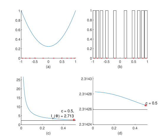
Figure 1: Jittered design for an approximately linear univariate response using $\nu=.5$, $c=.5$, $n=10$. (a) Minimax design density $m\left(x\right)$ and $\left\{t_{i}\right\}_{i=1}^{n}$. (b) Sampling density $\phi\left(x;c\right)$. (c) $I_{\nu}\left(\Phi\right)$ vs. $c$; horizontal line at $I_{\nu}\left(\xi\right)=2.314$. (d) qimse$\left(\Phi|\psi_{\ast}\right)$ vs. $c$; horizontal line at qimse$\left(\xi|\psi_{\ast}\right)=I_{\nu}\left(\xi\right)$.

A comparison of the maximum loss (5) of $\xi$ versus that of the design measure $\Phi$ corresponding to $\phi$ is obtained from

$$I_{\nu}\left(\xi\right) = 2\left(1-\nu\right)\left(1+\frac{1}{3\mu_{2}(\alpha)}\right)+\nu\left(1+\frac{5}{4}\left(3\mu_{2}(\alpha)-1\right)^{2}\right),$$

$$I_{\nu}\left(\Phi\right) = 2\left(1-\nu\right)\left(1+\frac{1}{3\lambda_{2}(c)}\right)+\frac{\nu}{c}\max\left(1,\frac{1}{3\lambda_{2}(c)}\right),$$

where

$$\mu_{2}(\alpha)=\frac{3-5\alpha}{5\left(1-3\alpha\right)},\text{ and }\lambda_{2}(c)=\int_{-1}^{1}x^{2}\phi\left(x;c\right)dx=\frac{1}{n}\sum_{i=1}^{n}t_{i}^{2}+\frac{c^{2}}{3n^{2}}.$$

Note that $I_{\nu}\left(\Phi\right)$ is evaluated at the least favourable contaminant $\psi_{\Phi}$, determined as at (7) with $\xi$ replaced by $\Phi$.

See Figure 1, where we present plots and comparative values, when placing equal weight on protection against bias versus variance ($\nu=.5$), $50\%$ of the design space to be sampled from $\Phi$ ($c=.5$) and $n=10$.

In Figure 1(d) we give values of the loss (4) against a particular $\psi$ of interest. With these designs the alternative of most concern is probably quadratic, and so we take $\psi(x)=\left(\tau/\sqrt{n}\right)\psi_{\ast}(x)$, with $\psi_{\ast}(x)=\sqrt{45/8}\left(x^{2}-1/3\right)$, orthogonal to $\left(1,x\right)$ and having $\int_{-1}^{1}$ $\psi_{\ast}^{2}(x)dx=1$. From (7) we see that this in fact gives the least favourable contaminant for the design $\xi$.

For any symmetric design $\pi$ with $\mu_{2}\left(\pi\right)=$ $\int_{-1}^{1}x^{2}\pi\left(dx\right)$, the loss (4) applied to this quadratic alternative is $\left(\sigma_{\varepsilon}^{2}+\tau^{2}\right)/n$ times

$$\text{{qimse}}\left(\pi|\psi_{\ast}\right) = \left(1-\nu\right)tr\left(\boldsymbol{AM}_{\pi}^{-1}\right)+\nu\left(\boldsymbol{b}_{\psi_{\ast},\pi}^{\boldsymbol{\prime}}\boldsymbol{M}_{\pi}^{-1}\boldsymbol{AM}_{\pi}^{-1}\boldsymbol{b}_{\psi_{\ast},\pi}+1\right)$$

$$= 2\left(1-\nu\right)\left(1+\frac{1}{3\mu_{2}\left(\pi\right)}\right)+\nu\left(\frac{5}{4}\left(3\mu_{2}\left(\pi\right)-1\right)^{2}+1\right).$$

In Figure 1(d) we plot qimse$\left(\Phi|\psi_{\ast}\right)$ and highlight qimse$\left(\xi|\psi_{\ast}\right)$, which by virtue of the observation above coincides with $I_{\nu}\left(\xi\right)$.

As noted in §2.1, $E_{\Phi}\left[\text{{imse}}\left(\delta|\psi_{\Phi}\right)\right]$ simplifies considerably for these jittered designs and then $J_{\nu}\left(\Phi\right)$ is very similar to $I_{\nu}\left(\Phi\right)$. We show in the Appendix that in this case (9) becomes

$$J_{\nu}\left(\Phi\right)=\left(1-\nu\right)E_{\Phi}\left[tr\boldsymbol{AM}_{\delta}^{-1}\right]+\frac{\nu}{c}\max\left(1,\frac{1}{3\lambda_{2}\left(c\right)}\right).$$ (12)

We note that

$$E_{\Phi}\left[tr\boldsymbol{AM}_{\delta}^{-1}\right]=2\left\{1+E_{\Phi}\left[\frac{\mu_{\delta}^{2}+\frac{1}{3}}{\sigma_{\delta}^{2}}\right]\right\},$$

where $\mu_{\delta}$ and $\sigma_{\delta}^{2}$ are the mean and variance of the design.

From both (c) and (d) of Figure 1 we see that the loss associated with the design $\Phi$ decreases with $c$, i.e. as the design becomes closer to the uniform design on all of $\chi$, for which the bias vanishes. This is in line with the remark of Box and Draper (1959): “The optimal design in typical situations in which both variance and bias occur is very nearly the same as would be obtained if variance were ignored completely and the experiment designed so as to minimize bias alone.”

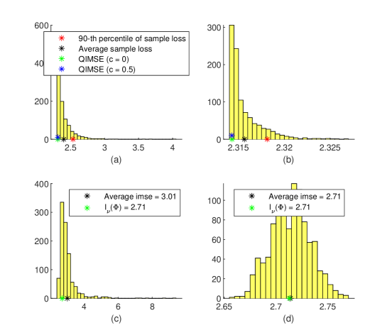
Figure 2: Top: Values of qimse from 1000 simulated random designs. Bottom: Values of imse$\left(\delta|\psi_{\Phi}\right)$ and their average, estimating $E\left[\text{{imse}}\left(\delta|\psi_{\Phi}\right)\right]$. These use the same inputs as in Figure 1. (a), (c): Completely random sampling. (b), (d): Stratified random sampling.

Table 1. Descriptive measures in Figure 2 (a), (b).
qimse $(c=0)=2.3143$.
Measure	Sampling method
	(a) Completely random	(b) Stratified
90th percentile	2.5092	2.3145
Average loss∗	2.3985	2.3143
∗Expected loss is qimse (c =  .5) = 2.3143. The very slight difference between
this and qimse (c = 0) can be discerned from Figure 1.

3.1.1 Sampling methods

We simulated $M=1000$ completely random and stratified random designs, in order to assess their performance. A completely random design consisted of $n=10$ points chosen from $\phi\left(x;c\right)$. Stratification consisted of choosing one design point at random from each bin. In each case we plotted qimse$\left(\pi|\psi_{\ast}\right)$ (calculated using $\mu_{2}\left(\pi\right)=\sum_{i=1}^{n}x_{i}^{2}/n$), and then evaluated various descriptive measures. See Figure 2(a),(b). As was seen in Figure 1 and Table 1 there is a negligible difference in qimse when going from the discrete design with $c=0$, to its randomization with $c=.5$, even though the former has infinite maximum loss. The sample averages of the losses from the randomized designs were smaller and closer to their expectation qimse$\left(\Phi|\psi_{\ast}\right)$ under the stratified sampling scheme, and the losses themselves were much more concentrated near qimse$\left(\Phi|\psi_{\ast}\right)$, as exhibited by the much shorter tail in (b). Similar comments apply to the values of imse$\left(\delta|\psi_{\Phi}\right)$ in Figure 2(c),(d). In a further calculation, for which the output is not displayed here, we estimated $J_{\nu}\left(\xi\right)$, as at (9), by drawing $1000$ samples from the minimax density $m\left(x\right)$ and computing imse$\left(\delta|\psi_{\xi}\right)$ for each. The values showed even more variation than those plotted in Figure 5(c), but with an average imse of $2.72$ – very close to that in Figure 5(d). From this we infer that jittering combined with stratification gives an efficient, structured implementation of the minimax solution.

Simulations using other inputs also resulted in these same conclusions – that our random design strategies typically yield designs very close to optimal with respect to our robustness and efficiency requirements, and that do not suffer from the drawback of deterministic designs of having infinite maximum loss.

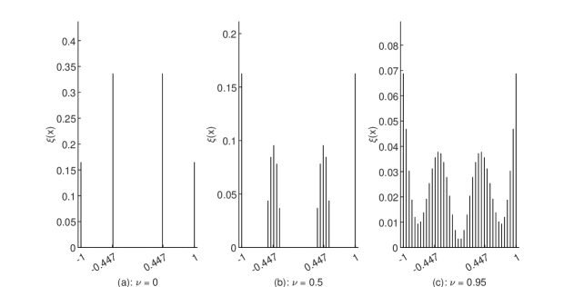
Figure 3: Minimax designs for approximate cubic regression

4 Cluster designs in one dimension

Working in discrete design spaces, Wiens (2018) obtained minimax robust designs for a variety of approximate responses. Those shown in Figure 3 are for cubic regression.  The classically I-optimal design ($\nu=0$) minimizing integrated variance alone was derived by Studden (1977) and places masses of $.1545$ and $.3455$ at $\pm 1$ and $\pm.4472$. The robust designs can thus be described as taking the replicates of the classical design and spreading their mass out (‘clustering’) over nearby regions. This same phenomenon has frequently been noticed in other situations (Fang and Wiens 2000, Heo, Schmuland and Wiens 2001 for instance).

In this section we aim to formalize this notion in order to obtain designs competing with the minimax designs, but with finite maximum loss even in continuous design spaces, and having the advantage of being much more easily derived – there is no need for the minimax designs to be known. We consider only one-dimensional designs in this section, and will illustrate the methods in polynomial response models of degrees $p-1=1,2,3$.

Suppose that a given static design has $p$ support points $t_{1}<\cdot\cdot\cdot<t_{p}$ in $[-1,1]$. Define midpoints $s_{i}=\left(t_{i}+t_{i+1}\right)/2$, $i=1,\cdot\cdot\cdot,p-1$. Put $s_{0}=\min$ $\left(-1,t_{1}\right)$ and $s_{p}=\max\left(1,t_{p}\right)$. Then the $p$ intervals $I_{i}=\left\{\left[s_{i-1},s_{i}\right],\text{ }i=1,...,p\right\}\$cover $[-1,1]$ and have the properties that $t_{i}\in I_{i}$ and that any point in $I_{i}$ is closer to $t_{i}$ than to any $t_{j}$, $j\neq i$. We note that this is then a trivial example of a Voronoi tessellation, to be considered when we pass to higher dimensions.

We propose designs consisting of points sampled from Beta densities on subintervals of the $I_{i}$. Specifically, for $i=1,...,p$ let $c=c\left(\nu\right)\in\left[0,1\right]$ satisfy $c\left(0\right)=0$ and $c\left(1\right)=1$. Put $J_{i}\left(c\right)=\left[t_{i}-c\left(t_{i}-s_{i-1}\right),t_{i}+c\left(s_{i}-t_{i}\right)\right]\equiv\left[k_{i},l_{i}\right]$, with length $\left|J_{i}\right|=\left(l_{i}-k_{i}\right)=c\left(s_{i}-s_{i-1}\right)=c$ $\times\left|I_{i}\right|$. Let $\beta_{a,b}\left(x\right)$ be the Beta$\left(a,b\right)$ density on $\left[0,1\right]$. Then

$$\frac{1}{\left|J_{i}\right|}\beta_{a,b}\left(\frac{x-k_{i}}{\left|J_{i}\right|}\right),\text{ }x\in J_{i}\left(c\right)$$ (13)

is this density, translated and scaled to$\ J_{i}\left(c\right)$. The interpretation of ‘$c$’ is as before – it is the fraction of the design space to be sampled.

The parameters $\left(a_{i},b_{i}\right)$ are chosen so that the mode of (13) is at $t_{i}\in J_{i}\left(c\right)$, hence the mode $\delta_{i}\in\left[0,1\right]$ of $\beta_{a,b}\left(x\right)$ is given by

$$\delta_{i}\equiv\frac{t_{i}-k_{i}}{l_{i}-k_{i}}=\left\{\begin{tabular}[]{cc}$\frac{a_{i}-1}{a_{i}-1+b_{i}-1},$&$a_{i},b_{i}>1,$\\ $0,$&$a_{i}\leq 1<b_{i},$\\ $1,$&$b_{i}\leq 1<a_{i}.$\end{tabular}\right.$$

Then

$$\left(a_{i}-1\right)\left(1-\delta_{i}\right)=\left(b_{i}-1\right)\delta_{i}.$$ (14)

If $\delta_{i}\neq 0,1$ we determine one of $\left(a_{i},b_{i}\right)$ in terms of the other through (14). If $-1=t_{1}$ then $\delta_{1}=0$ and we set $a_{1}=1$. If $t_{p}=1$ then $\delta_{p}=1$ and we set $b_{p}=1$. In each case the remaining parameter is set equal to $1/\nu$, so that the density tends to a point mass at $t_{i}$ as $\nu\rightarrow 0$ and to uniformity as $\nu\rightarrow 1$. Correspondingly we choose $c\left(\nu\right)=\nu$.

The final density $\phi\left(\cdot\right)$ from which the design points are to be sampled is a weighted average of those at (13), with weights proportional to the lengths $\left|I_{i}\right|$ of the $I_{i}$. Since $\left|J_{i}\right|=c\left|I_{i}\right|$ we obtain

$$\phi\left(x;\nu\right)=\frac{1}{2c}\sum_{i=1}^{p}\beta_{a_{i},b_{i}}\left(\frac{x-k_{i}}{\left|J_{i}\right|}\right)I\left(x\in J_{i}\right).$$ (15)

Motivated by the designs of §3.1 we recommend stratified sampling, by which the sample consists of $\approx n\left|I_{i}\right|/2$ points drawn from (13), subject to an appropriate rounding procedure.

Table 2.  Performance measures for the designs of Figure 4.
	variance			max sqd. bias			$I_{\nu}$
	$\nu=.5$	$\nu=.04$		$\nu=.5$	$\nu=.04$		$\nu=.5$	$\nu=.04$
$p=2$	$2.94$	$2.67$		$2.67$	$319$		$2.80$	$15.3$
$p=3$	$4.65$	$4.27$		$2.62$	$213$		$3.64$	$12.6$
$p=4$	$6.49$	$6.02$		$2.54$	$193$		$4.51$	$13.5$

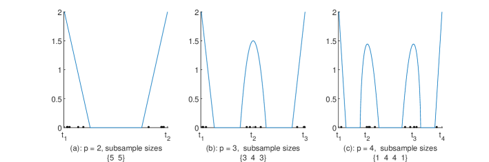
Figure 4: Cluster design densities $\phi\left(x;\nu=.5\right)$; typical stratified samples using weights (a) $\left\{.5,.5\right\}$, (b) $\left\{.25,.5,.25\right\}$, (c) $\left\{.14,.36,.36,.14\right\}$.

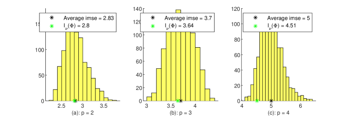
Figure 5: Values of imse$\left(\delta|\psi_{\Phi}\right)$ from $1000$ simulated random designs for polynomial regression and their average, estimating $E\left[\text{{imse}}\left(\delta|\psi_{\Phi}\right)\right]$.

4.1 Polynomial regression

We illustrate these proposals in the context of approximate polynomial responses of degrees $p-1=1,2,3$. As also suggested in ‘Heuristic 5.1’ of Waite and Woods (2022, p. 1462), $t^{\ast}$ will consist of the support points of the classical I-optimal designs. These I-optimal designs $\xi^{\ast}$ are obtained from Lemma 3.2 of Studden (1977), and are as follows.

$p=2$: $\xi^{\ast}\left(\pm 1\right)=.5$,

$p=3$: $\xi^{\ast}\left(\pm 1\right)=.25$, $\xi^{\ast}\left(0\right)=.5$,

$p=4$: $\xi^{\ast}\left(\pm 1\right)=\frac{1}{2\left(1+\sqrt{5}\right)}\approx.1545$, $\xi^{\ast}\left(\pm\frac{1}{\sqrt{5}}\approx\pm.4472\right)=\frac{\sqrt{5}}{2\left(1+\sqrt{5}\right)}\approx.3455$.

Figure 4 gives the sampling densities (15), together with the subsample sizes when $n=10$. Figure 4(a) gives output for the approximate linear model, with a maximum imse, as at (5), of $I_{\nu}\left(\Phi\right)=$ $2.8039$. This compares very favourably with the design of Figure 1, especially given that its construction does not require the minimax design to be given. This latter point is especially germane for the design of Figure 4(b), since it is the analogue of the absolutely continuous minimax designs for approximate quadratic regression derived – with substantial theoretical and computational difficulty – by Shi, Ye and Zhou (2003) using methods of non-smooth optimization and by Daemi and Wiens (2013) using completely different methods.

Figure 5 gives simulated values of imse$\left(\delta|\psi_{\Phi}\right)$ from $1000$ simulated random designs, together with their average, estimating $E\left[\text{{imse}}\left(\delta|\psi_{\Phi}\right)\right]$. On average the random designs perform almost as well against $\psi_{\Phi}$ as the continuous design $\Phi$.

It is interesting to note – especially for the design of Figure 4(c) – the close agreement between the I-optimal design weights above, and the weights used in the computation of $\phi$.

See Table 2, where the variance and maximum squared bias components of $I_{\nu}$ are presented for the designs of Figure 4 ($\nu=.5$) and for the corresponding designs with $\nu=.04$, very closely approximating the I-optimal design ($\nu=0$) with maximum loss $I_{0}=\infty$. That the robustness of the cluster designs is achieved for such a modest premium in terms of increased variance is both startling and encouraging.

5 Multidimensional cluster designs

Figure 6: Design for fitting a full second order model; $n=48$.

See Figure 6, where a robust design, derived for fitting a full second order bivariate model – intercept, linear, quadratic and interaction terms – is depicted. It is a discrete implementation of a design density, optimally robust against model misspecifications in a certain parametric class of densities – see Heo, Schmuland and Wiens (2001) for details. This design can roughly be described as an inscribed Central Composite Design (CCD) with ‘clustering’ in place of replication. It serves as motivation for the ideas of this section, which we illustrate in the context of $k$-dimensional, spherical CCD designs as are often used to fit second order models. Such designs utilize $2^{k}+2k+1$ points $\left\{\boldsymbol{t}_{i}\right\}$ consisting of $2^{k}$ corner points with $\boldsymbol{t}_{i,j}=\pm 1$ ($j=1,...,k$), $2k$ axial points $\boldsymbol{t}_{i}=\left(0,...,\pm\sqrt{k},...,0\right)$ and a centre point $\boldsymbol{t}_{i}=\left(0,...,0,...,0\right)$.

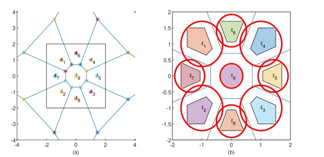
Figure 7: (a) Voronoi tessellation generated by the points $\left\{\boldsymbol{t}_{i}\right\}$. (b) Tessellation restricted to $\chi=\left[-2,2\right]^{2}$ with subtiles $\left\{J_{i}\left(.25\right)\right\}$ and enclosing circles $\left\{\mathcal{S}^{\left(2\right)}\left(\boldsymbol{t}_{i},R_{i}\right)\right\}$.

In this and other multidimensional cases we propose choosing design points from spherical densities concentrated on neighbourhoods of the $\boldsymbol{t}_{i}$. A spherical density on a $k$-dimensional hypersphere

$$\mathcal{S}^{\left(k\right)}\left(\boldsymbol{t},R\right)=\left\{\boldsymbol{x}\left|\left\|\boldsymbol{x}-\boldsymbol{t}\right\|\leq R\right.\right\}$$

with centre $\boldsymbol{t}$ and radius $R$, in which the norm $\left\|\boldsymbol{x}-\boldsymbol{t}\right\|$ has a scaled $Beta\left(1,b\right)$ density, is given by

$$f^{(k)}\left(\boldsymbol{x};\boldsymbol{t},R,b\right)=\frac{\Gamma\left(\frac{k}{2}\right)}{2\pi^{k/2}R^{k}}\cdot\frac{b\left(1-\frac{\left\|\boldsymbol{x}-\boldsymbol{t}\right\|}{R}\right)^{b-1}}{\left(\frac{\left\|\boldsymbol{x}-\boldsymbol{t}\right\|}{R}\right)^{k-1}}I\left(\boldsymbol{x}\in\mathcal{S}^{\left(k\right)}\left(\boldsymbol{t},R\right)\right).$$

Such a density has mode $\boldsymbol{t}$ and approaches a point mass at $\boldsymbol{t}$ as $b\rightarrow\infty$, and uniformity as $b\rightarrow 1$.

A sample value $\boldsymbol{x}$ from $f^{(k)}\left(\boldsymbol{x};\boldsymbol{t},R,b\right)$ is $\boldsymbol{x=t}+\boldsymbol{Ry}$, where $\boldsymbol{y}\sim f^{(k)}\left(\boldsymbol{\cdot};\boldsymbol{0},1,b\right)$ is obtained by drawing a value of $\rho=\left\|\boldsymbol{y}\right\|\sim Beta(1,b)$ and, independently, drawing angles $\theta_{i}$, $-\pi/2<\theta_{i}\leq\pi/2$ ($i=1,...,k-2$)  with densities $\psi_{i}\left(\theta\right)=\cos^{k-i-1}\theta\left/\beta\left(1/2,\left(k-i\right)/2\right)\right.$ – equivalently, $\cos^{2}\theta_{i}$ $\sim Beta(\frac{1}{2},\frac{k-i}{2})$ – and $\theta_{k-1}\sim Unif\left(-\pi,\pi\right)$. Then

$$y_{1} = \rho\sin\theta_{1},$$

$$y_{2} = \rho\cos\theta_{1}\sin\theta_{2},$$

$$y_{3} = \rho\cos\theta_{1}\cos\theta_{2}\sin\theta_{3},$$

$$\cdot\cdot\cdot$$

$$y_{k-1} = \rho\cos\theta_{1}\cos\theta_{2}\cdot\cdot\cdot\cos\theta_{k-2}\sin\theta_{k-1},$$

$$y_{k} = \rho\cos\theta_{1}\cos\theta_{2}\cdot\cdot\cdot\cos\theta_{k-2}\cos\theta_{k-1}.$$

To sample $\theta_{i}$ for $i<k-1$ we draw $z\sim Beta(\frac{1}{2},\frac{k-i}{2})$ and set $\theta_{i}=\pm\arccos\sqrt{z}$, each with probability $1/2$.

5.1 Two dimensional cluster designs on tessellations

Figure 8: Sampling density $\phi\left(\boldsymbol{x};\nu=.5\right)$ constructed for a robust, clustered CCD in two dimensions.

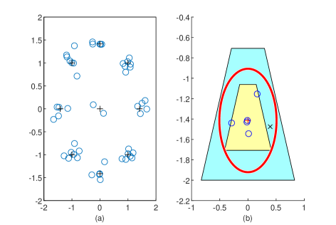
Figure 9: (a) A typical random CCD of size 50; $\nu=.5$. (b) Details of the subsample of 5 points (‘o’) drawn from $J_{8}\left(.25\right)$. Rejected points are marked as ‘x’.

In Figure 7(a), the nine points $\left\{\boldsymbol{t}_{i}\right\}$ which are displayed consist of four corner points $(-1,\pm 1)$, $(1,\pm 1)$, four axial points $\left(\pm\sqrt{2},0\right)$, $\left(0,\pm\sqrt{2}\right)$ and the centre point $\left(0,0\right)$. These are the generators of the Voronoi tessellation pictured - a tiling with the property that, within the tile $T_{i}$ containing $\boldsymbol{t}_{i}$, all points are closer to $\boldsymbol{t}_{i}$ than to any $\boldsymbol{t}_{j},$ $j\neq i$. Figure 7(b) gives a more detailed depiction of the tessellation, restricted to the design space $\chi=\left[-2,2\right]\times[-2,2]$. Within each tile $T_{i}$, of area $\left|T_{i}\right|$, we have also plotted a subtile $J_{i}\left(c\right)$ which is a contraction of $T_{i}$ with fixed point $\boldsymbol{t}_{i}$ and area $\left|J_{i}\left(c\right)\right|=c\left|T_{i}\right|$. These are then the analogues of the subintervals $J_{i}\left(c\right)\subseteq I_{i}$ from §4, and ‘$c$’ has the same interpretation – the fraction of the design space to be sampled. Surrounding each $J_{i}\left(c\right)$ is the smallest enclosing circle $\mathcal{S}^{\left(2\right)}\left(\boldsymbol{t}_{i},R_{i}\left(c\right)\right)$.

We sample design points from $\mathcal{S}^{\left(2\right)}\left(\boldsymbol{t}_{i},R_{i}\left(c\right)\right)$, accepting only those points which lie in $J_{i}\left(c\right)$. We specify $b=1/\nu$ and $c=\nu^{2}$, then $f^{(2)}\left(\boldsymbol{x};\boldsymbol{t}_{i},R_{i}\left(c\right),b\right)$ approaches a point mass at $\boldsymbol{t}_{i}$ as $\nu\rightarrow 0$, and uniformity on $\mathcal{S}^{\left(2\right)}\left(\boldsymbol{t}_{i},R_{i}\left(c\right)\right)\supseteq T_{i}$ as $\nu\rightarrow 1$.  With

$$q_{i}(\nu)=\int_{J_{i}\left(c\right)}f^{(2)}\left(\boldsymbol{x};\boldsymbol{t}_{i},R_{i}\left(c\right),b\right)\mu\left(d\boldsymbol{x}\right),$$

the density of those points accepted into the design upon being drawn from $\mathcal{S}^{\left(2\right)}\left(\boldsymbol{t}_{i},R_{i}\left(c\right)\right)$ is

$$\frac{f^{(2)}\left(\boldsymbol{x};\boldsymbol{t}_{i},R_{i}\left(c\right),b\right)}{q_{i}(\nu)}I\left(\boldsymbol{x}\in J_{i}\left(c\right)\right).$$

We again do stratified sampling, with weights $\omega_{i}=\left|T_{i}\right|\left/\sum\left|T_{i}\right|\right.$ proportional to the area $\left|T_{i}\right|$, whence the density of the design on $\chi$ is

$$\phi\left(\boldsymbol{x};\nu\right)=\sum_{i=1}^{9}\frac{\omega_{i}}{q_{i}(\nu)}f^{(2)}\left(\boldsymbol{x};\boldsymbol{t}_{i},R_{i}\left(c\right),b\right)I\left(\boldsymbol{x}\in J_{i}\left(c\right)\right).$$

See Figure 8. Although we evaluate $q_{i}(\nu)$ by numerical integration, an estimate can be computed after the sampling is done; it is the proportion of those points which were drawn from $\mathcal{S}^{\left(2\right)}\left(\boldsymbol{t}_{i},R_{i}\left(c\right)\right)$ and then accepted into the sample. This estimate turns out to be quite accurate if an artificially large sample is simulated.

Figure 9 illustrates the results of applying the methods of the preceding discussion. We chose a total sample size of $n=50$, $\nu=.5$, and obtained subsample sizes $n_{i}=n\omega_{i}$, rounded to $\left\{7,7,7,7,5,5,5,5,2\right\}$ with each corner point being allocated $7$, each axial point being allocated $5$, and the remaining $2$ in the centre. The entire sample is shown in Figure 9(a), with Figure 9(b) illustrating the details for Tile $8$. The required $5$ points were found after $6$ points were drawn from $\mathcal{S}_{8}$. In all, $7$ points were rejected as not belonging to the appropriate subtile.

5.2 Extensions to $k>2$

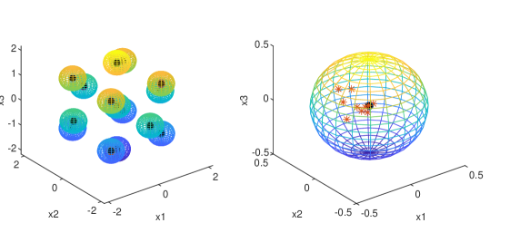
Figure 10: (a) Spheres $\mathcal{S}^{\left(3\right)}\left(\boldsymbol{t}_{i},r_{0}\nu\right)$, $i=1,...,15$ for a three dimensional spherical CCD and $\nu=.5$. (b) Centre sphere $\mathcal{S}^{\left(3\right)}\left(\boldsymbol{0},r_{0}\nu\right)$ with sampled points.

Although the theory of §5.1 extends readily to higher dimensions, the lack of appropriate software for constructing and manipulating Voronoi tessellations becomes a severe drawback. But the general idea of sampling from spherical distributions centred on small neighbourhoods of the $\left\{\boldsymbol{t}_{i}\right\}$ can still be applied, albeit in a less structured manner.

Let $\left\{\boldsymbol{t}_{i}\right\}_{i=1}^{q}$ be the $q=2^{k}+2k+1$ support points of a spherical CCD  in variables $\boldsymbol{x}=\left(x_{1},...,x_{k}\right)^{\prime}$, as described at the beginning of this section. The minimum distance between these points is $\min\left(2,\sqrt{k}\right)$, and so hyperspheres $\mathcal{S}\left(\boldsymbol{t}_{i},r_{0}\right)$ centred at the $\boldsymbol{t}_{i}$ and with radius $r_{0}=\min\left(1,\sqrt{k}/2\right)$ are disjoint.  Define subspheres

$$J_{i}\left(c\right)=\mathcal{S}^{\left(k\right)}\left(\boldsymbol{t}_{i},r_{0}c^{1/k}\right),0<c\leq 1.$$

Then $\int I\left(\boldsymbol{x}\in J_{i}\left(c\right)\right)d\boldsymbol{x}=\left|J_{i}\left(c\right)\right|=c\left|\mathcal{S}\left(\boldsymbol{t}_{i},r_{0}\right)\right|$. The density of $\boldsymbol{x}$ on $J_{i}\left(c\right)$ is $f^{(k)}\left(\boldsymbol{\cdot};\boldsymbol{t}_{i},r_{0}c^{1/k},b\right)$. We again specify $b=1/\nu$ and set $c=\nu^{k}$. Then for user chosen weights $\left\{\omega_{i}\right\}$ the sampling density is

$$\phi\left(\boldsymbol{x};\nu\right)=\sum_{i=1}^{q}\omega_{i}f^{(k)}\left(\boldsymbol{x};\boldsymbol{t}_{i},r_{0}\nu,1/\nu\right)I\left(\boldsymbol{x}\in\mathcal{S}^{\left(k\right)}\left(\boldsymbol{t}_{i},r_{0}\nu\right)\right).$$

See Figure 10 for an example with $k=3$. We sampled a design of size $n=80$ with subsample sizes $n_{i}=5$ ($i<15$) and $n_{15}=10$.

Appendix

A.1 Derivations for §2.1

For an  $n$-point design $D=\left\{\boldsymbol{x}_{i}\right\}_{i=1}^{n}$ with design measure $\delta=n^{-1}\sum\delta_{\boldsymbol{x}_{i}}$ define

$$\boldsymbol{F}=\left(\boldsymbol{f}\left(\boldsymbol{x}_{1}\right),\cdot\cdot\cdot,\boldsymbol{f}\left(\boldsymbol{x}_{n}\right)\right)^{\prime},\boldsymbol{\psi}_{\Phi}=\left(\psi_{\Phi}\left(\boldsymbol{x}_{1}\right),...,\psi_{\Phi}\left(\boldsymbol{x}_{n}\right)\right)^{\prime},\text{ }\boldsymbol{D}_{\phi}=diag\left(\phi\left(\boldsymbol{x}_{1}\right),...,\phi\left(\boldsymbol{x}_{n}\right)\right).$$

Then $\boldsymbol{M}_{\phi}=\frac{1}{n}\boldsymbol{F}^{\prime}\boldsymbol{D}_{\phi}\boldsymbol{F}$. Define as well

$$\boldsymbol{M}_{\delta} = \int_{\chi}\boldsymbol{f}\left(\boldsymbol{x}\right)\boldsymbol{f}^{\prime}\left(\boldsymbol{x}\right)\delta\left(d\boldsymbol{x}\right)=\frac{1}{n}\sum_{\boldsymbol{x}_{i}\in D}\boldsymbol{f}\left(\boldsymbol{x}_{i}\right)\boldsymbol{f}^{\prime}\left(\boldsymbol{x}_{i}\right)=\frac{1}{n}\boldsymbol{F}^{\prime}\boldsymbol{F},\text{ \ }$$

$$\boldsymbol{b}_{\psi_{\Phi},\delta} = \int_{\chi}\boldsymbol{f}\left(\boldsymbol{x}\right)\psi_{\Phi}\left(\boldsymbol{x}\right)\delta\left(d\boldsymbol{x}\right)=\frac{1}{n}\sum_{\boldsymbol{x}_{i}\in D}\boldsymbol{f}\left(\boldsymbol{x}_{i}\right)\psi_{\Phi}\left(\boldsymbol{x}_{i}\right)=\frac{1}{n}\boldsymbol{F}^{\prime}\boldsymbol{\psi}_{\Phi}.$$

Using (7),

$$\psi_{\Phi}\left(\boldsymbol{x}_{i}\right)=\mathbf{r}_{\Phi}^{\prime}\left(\boldsymbol{x}_{i}\right)\mathbf{\beta}_{\Phi}=\frac{\tau}{\sqrt{n}}\left(\phi\left(\boldsymbol{x}_{i}\right)\boldsymbol{f}^{\prime}\left(\boldsymbol{x}_{i}\right)-\boldsymbol{f}^{\prime}\left(\boldsymbol{x}_{i}\right)\boldsymbol{A}^{-1}\boldsymbol{M}_{\Phi}\right)\boldsymbol{G}_{\Phi}^{-1/2}\mathbf{\beta}_{\Phi}\mathbf{,}$$

so that

$$\boldsymbol{\psi}_{\Phi} = \frac{\tau}{\sqrt{n}}\left(\boldsymbol{D}_{\phi}\boldsymbol{F}\mathbf{-}\boldsymbol{FA}^{-1}\boldsymbol{M}_{\Phi}\right)\boldsymbol{G}_{\Phi}^{-1/2}\mathbf{\beta}_{\Phi}\mathbf{,}$$ (A.1)

$$\boldsymbol{b}_{\psi_{\Phi},\delta} = \frac{\tau}{\sqrt{n}}\left(\boldsymbol{M}_{\phi}-\boldsymbol{M}_{\delta}\boldsymbol{A}^{-1}\boldsymbol{M}_{\Phi}\right)\boldsymbol{G}_{\Phi}^{-1/2}\mathbf{\beta}_{\Phi}\mathbf{.}$$ (A.2)

From (4),

$$\text{{imse}}\left(\delta|\psi_{\Phi}\right)=\frac{\sigma_{\varepsilon}^{2}}{n}tr\left(\boldsymbol{AM}_{\delta}^{-1}\right)+\boldsymbol{b}_{\psi_{\Phi},\delta}^{\boldsymbol{\prime}}\boldsymbol{M}_{\delta}^{-1}\boldsymbol{AM}_{\delta}^{-1}\boldsymbol{b}_{\psi_{\Phi},\delta}+\int_{\chi}\psi_{\Phi}^{2}\left(x\right)\mu\left(dx\right);$$

substituting (A.1) and (A.2) gives

$$\text{{imse}}\left(\delta|\psi_{\Phi}\right) = \frac{\sigma_{\varepsilon}^{2}}{n}tr\left(\boldsymbol{AM}_{\delta}^{-1}\right)+\frac{\tau^{2}}{n}\gamma_{\delta},\text{ for}$$

$$\gamma_{\delta} = \mathbf{\beta}_{\Phi}^{\prime}\boldsymbol{G}_{\Phi}^{-1/2}\left(\boldsymbol{M}_{\phi}\boldsymbol{M}_{\delta}^{-1}-\boldsymbol{M}_{\Phi}\boldsymbol{A}^{-1}\right)\boldsymbol{A}\left(\boldsymbol{M}_{\delta}^{-1}\boldsymbol{M}_{\phi}-\boldsymbol{A}^{-1}\leavevmode\nobreak\ \boldsymbol{M}_{\Phi}\right)\boldsymbol{G}_{\Phi}^{-1/2}\mathbf{\beta}_{\Phi}+1.$$

Now (8) and (9) are immediate.

A.2 Derivation of (12)

We need only evaluate $E_{\Phi}\left[\gamma_{\delta}\right]$. Since $\phi\left(x_{i}\right)\equiv\left(2c\right)^{-1}$ on its support, we have that $\boldsymbol{M}_{\phi}\boldsymbol{M}_{\delta}^{-1}=\left(2c\right)^{-1}\boldsymbol{I}_{2}$, so that (since $\mathbf{\beta}_{\Phi}^{\prime}\mathbf{\beta}_{\Phi}=1$)

$$\gamma_{\delta} = \mathbf{\beta}_{\Phi}^{\prime}\boldsymbol{G}_{\Phi}^{-1/2}\left(\frac{1}{2c}\boldsymbol{I}_{2}-\boldsymbol{M}_{\Phi}\boldsymbol{A}^{-1}\right)\boldsymbol{A}\left(\frac{1}{2c}\boldsymbol{I}_{2}-\boldsymbol{A}^{-1}\boldsymbol{M}_{\Phi}\right)\boldsymbol{G}_{\Phi}^{-1/2}\mathbf{\beta}_{\Phi}+1$$ (A.3)

$$= \mathbf{\beta}_{\Phi}^{\prime}\boldsymbol{G}_{\Phi}^{-1/2}\left(\frac{1}{4c^{2}}\boldsymbol{A}-\frac{1}{c}\boldsymbol{M}_{\Phi}+\boldsymbol{M}_{\Phi}\boldsymbol{A}^{-1}\boldsymbol{M}_{\Phi}\right)\boldsymbol{G}_{\Phi}^{-1/2}\mathbf{\beta}_{\Phi}+1$$

$$= \mathbf{\beta}_{\Phi}^{\prime}\boldsymbol{G}_{\Phi}^{-1/2}\left(\frac{1}{4c^{2}}\boldsymbol{A}-\frac{1}{c}\boldsymbol{M}_{\Phi}+\boldsymbol{H}_{\Phi}+\boldsymbol{G}_{\Phi}\right)\boldsymbol{G}_{\Phi}^{-1/2}\mathbf{\beta}_{\Phi}.$$

A calculation gives

$$\boldsymbol{G}_{\Phi}^{1/2}\boldsymbol{H}_{\Phi}^{-1}\boldsymbol{G}_{\Phi}^{1/2}+\boldsymbol{I}_{2}=\frac{1}{c}diag\left(1,\frac{1}{3\lambda_{2}\left(c\right)}\right),$$

so that the maximum eigenvalue is $ch_{\max}=\frac{1}{c}\max(1,\frac{1}{3\lambda_{2}\left(c\right)})$ and $\mathbf{\beta}_{\Phi}$ is the corresponding unit eigenvector.  We claim that

$$\gamma_{\delta}=ch_{\max},$$ (A.4)

from which (12) follows, since then $\gamma_{\delta}$ does not depend on the design and so is non-random.

To establish (A.4), use $\boldsymbol{A}=\boldsymbol{M}_{\Phi}\boldsymbol{H}_{\Phi}^{-1}\boldsymbol{M}_{\Phi}=4c^{2}\boldsymbol{K}_{\Phi}\boldsymbol{H}_{\Phi}^{-1}\boldsymbol{K}_{\Phi}$ and $\boldsymbol{M}_{\Phi}=2c\boldsymbol{K}_{\Phi}$ in (A.3) to obtain

$$\gamma_{\delta}=\mathbf{\beta}_{\Phi}^{\prime}\left[\boldsymbol{G}_{\Phi}^{-1/2}\left(\boldsymbol{K}_{\Phi}\boldsymbol{H}_{\Phi}^{-1}\boldsymbol{K}_{\Phi}-\boldsymbol{K}_{\Phi}\right)\boldsymbol{G}_{\Phi}^{-1/2}\right]\mathbf{\beta}_{\Phi}.$$

Substituting $\boldsymbol{K}_{\Phi}=\boldsymbol{G}_{\Phi}+\boldsymbol{H}_{\Phi}$, this becomes

$$\gamma_{\delta}=\mathbf{\beta}_{\Phi}^{\prime}\left[\boldsymbol{G}_{\Phi}^{1/2}\boldsymbol{H}_{\Phi}^{-1}\boldsymbol{G}_{\Phi}^{1/2}+\boldsymbol{I}_{2}\right]\mathbf{\beta}_{\Phi}=ch_{\max},$$

as required.

References

Bischoff, W. (2010), “An Improvement in the Lack-of-Fit Optimality of the (Absolutely) Continuous Uniform Design in Respect of Exact Designs,” in mODa 9 - Advances in Model-Oriented Design and Analysis, eds. Giovagnoli, G., Atkinson, A. and Torsney, B.

Box, G.E.P., and Draper, N.R. (1959), “A Basis for the Selection of a Response Surface Design,” Journal of the American Statistical Association, 54, 622-654.

Daemi, M., and Wiens, D.P. (2013), “Techniques for the Construction of Robust Regression Designs,” The Canadian Journal of Statistics, 41, 679-695.

Fang, K.T. & Wang, Y. (1994). Number-Theoretic Methods in Statistics. Chapman and Hall, London and New York.

Fang, Z., and Wiens, D.P. (2000), “Integer-Valued, Minimax Robust Designs for Estimation and Extrapolation in Heteroscedastic, Approximately Linear Models,” Journal of the American Statistical Association, 95, 807-818.

Heo, G., Schmuland, B., and Wiens, D.P. (2001), “Restricted Minimax Robust Designs for Misspecified Regression Models,” The Canadian Journal of Statistics, 29, 117-128.

Huber, P.J. (1975), “Robustness and Designs,” in: A Survey of Statistical Design and Linear Models, ed. J.N. Srivastava, Amsterdam: North Holland, pp. 287-303.

Shi, P., Ye, J., and Zhou, J. (2003), “Minimax Robust Designs for Misspecified Regression Models,” The Canadian Journal of Statistics, 31, 397-414.

Studden, W.J. (1977), “Optimal Designs for Integrated Variance in Polynomial Regression,” Statistical Decision Theory and Related Topics II, ed. Gupta, S.S. and Moore, D.S. New York: Academic Press, pp. 411-420.

Waite, T.W., and Woods, D.C. (2022),“Minimax Efficient Random Experimental Design Strategies With Application to Model-Robust Design for Prediction,” Journal of the American Statistical Association, 117, 1452-1465.

Wiens, D.P. (1990), “Robust, Minimax Designs for Multiple Linear Regression,” Linear Algebra and Its Applications, Second Special Issue on Linear Algebra and Statistics; 127, 327 - 340.

Wiens, D.P. (1992), “Minimax Designs for Approximately Linear Regression,” Journal of Statistical Planning and Inference, 31, 353-371.

Wiens, D.P. (2015), “Robustness of Design”, Chapter 20, Handbook of Design and Analysis of Experiments, Chapman & Hall/CRC.

Wiens, D.P. (2018), “I-Robust and D-Robust Designs on a Finite Design Space,” Statistics and Computing, 28, 241-258.

Xu, X., and Yuen, W.K. (2011), “Applications and Implementations of Continuous Robust Designs,” Communications in Statistics - Theory and Methods, 40, 969-988.