Quasi–hyperbolically symmetric $\gamma$-metric

Abstract

We carry out a systematic study on the motion of test particles in the region inner to the naked singularity of a quasi–hyperbolically symmetric $\gamma$-metric. The geodesic equations are written and analyzed in detail. The obtained results are contrasted with the corresponding results obtained for the axially symmetric $\gamma$-metric, and the hyperbolically symmetric black hole. As in this latter case, it is found that test particles experience a repulsive force within the horizon (naked singularity), which prevents them to reach the center. However in the present case this behavior is affected by the parameter $\gamma$ which measures the departure from the hyperbolical symmetry. These results are obtained for radially moving particles as well as for particles moving in the $\theta-r$ subspace. Possible relevance of these results in the explanation of extragalactic jets, is brought out.

I Introduction

In a recent paper 1 an alternative global description of the Schwarzschild black hole has been proposed. The motivation behind such an endeavor was, on the one hand the fact that the space–time within the horizon, in the classical picture, is necessarily non–static or, in other words, that any transformation that maintains the static form of the Schwarzschild metric (in the whole space–time) is unable to remove the coordinate singularity appearing on the horizon in the line element rosen . Indeed, as is well known, no static observers can be defined inside the horizon (see Rin ; Caroll for a discussion on this point). This conclusion becomes intelligible if we recall that the Schwarzschild horizon is also a Killing horizon, implying that the time–like Killing vector existing outside the horizon, becomes space–like inside it.

On the other hand, based on the physically reasonable point of view that any equilibrium final state of a physical process should be static, it would be desirable to have a static solution over the whole space–time.

Based on the arguments above, the following model was proposed in 1 .

Outside the horizon ($R>2M$) one has the usual Schwarzschild line element corresponding to the spherically symmetric vacuum solution to the Einstein equations, which in polar coordinate reads (with signature $+2$)

$$ds^{2} = -\left(1-\frac{2M}{R}\right)dt^{2}+\frac{dR^{2}}{\left(1-\frac{2M}{R}\right)}+R^{2}d\Omega^{2},$$

$$d\Omega^{2} = d\theta^{2}+\sin^{2}\theta d\phi^{2}.$$ (1)

This metric is static and spherically symmetric, meaning that it admits four Killing vectors:

$$\mathbf{\xi}_{(\mathbf{0})}=\partial_{\mathbf{t}},\quad{\bf\xi_{(2)}}=-\cos\phi\partial_{\theta}+\cot\theta\sin\phi\partial_{\phi},$$

$${\bf\xi_{(1)}}=\partial_{\phi},\quad{\bf\xi_{(3)}}=\sin\phi\partial_{\theta}+\cot\theta\cos\phi\partial_{\phi}.$$ (2)

The solution proposed for $R<2M$ (with signature $-2$) is

$$ds^{2} = \left(\frac{2M}{R}-1\right)dt^{2}-\frac{dR^{2}}{\left(\frac{2M}{R}-1\right)}-R^{2}d\Omega^{2},$$

$$d\Omega^{2} = d\theta^{2}+\sinh^{2}\theta d\phi^{2}.$$ (3)

This is a static solution, meaning that it admits the time–like Killing vector $\mathbf{\xi}_{(\mathbf{0})}$, however unlike (1) it is not spherically symmetric, but hyperbolically symmetric, meaning that it admits the three Killing vectors

$${\bf\chi_{(2)}}=-\cos\phi\partial_{\theta}+\coth\theta\sin\phi\partial_{\phi},$$

$${\bf\chi_{(1)}}=\partial_{\phi},\quad{\bf\chi_{(3)}}=\sin\phi\partial_{\theta}+\coth\theta\cos\phi\partial_{\phi}.$$ (4)

Thus if one wishes to keep sphericity within the horizon, one should abandon staticity, and if one wishes to keep staticity within the horizon, one should abandon sphericity.

The classical picture of the black hole entails sphericity within the horizon, instead in 1 we have proceeded differently and have assumed staticity within the horizon.

The three Killing vectors (4) define the hyperbolical symmetry. Space–times endowed with hyperbolical symmetry have previously been the subject of research in different contexts (see Ha –hn5 and references therein).

In 2nc a general study of geodesics in the spacetime described by (3) was presented (see also Lim ), leading to some interesting conclusions about the behavior of a test particle in this new picture of the Schwarzschild black hole, namely:

• the gravitational force inside the region $R<2M$ is repulsive.

• test particles cannot reach the center.

• test particles can cross the horizon outward, but only along the $\theta=0$ axis.

These intriguing results reinforces further the interest on this kind of systems.

The procedure used in 1 to obtain (3) may be used to obtain hyperbolic versions of other spacetimes. Of course in this case the obtained metric may not admit all the Killing vectors describing the hyperbolical symmetry (4), and it will not describe a black hole but a naked singularity. We shall refer to these space–times as quasi–hyperbolical.

It is the purpose of this work to delve deeper into this issue, by considering a specific quasi– hyperbolical space–time. Thus we shall analyze the quasi–hyperbolical version of the $\gamma$-metric Bach ; Vor ; WE ; Duncan . In particular we endeavor to analyze the geodesic structure of this space–time, and to contrast it with the corresponding geodesics of the hyperbolically symmetric version of the Schwarzschild metric discussed in 2nc and with the geodesic structure of the $\gamma$-metric discussed in gammas .

The motivation for this choice is twofold, on the one hand the $\gamma$-metric corresponds to a solution of the Laplace equation, in cylindrical coordinates, with the same Newtonian source image Bonnor as the Schwarzschild metric (a rod). On the other hand, it has been proved Herrera1 that by extending the length of the rod to infinity one obtains the Levi–Civita spacetime. At the same time a link was established between the parameter $\gamma$, measuring the mass density of the rod in the $\gamma$-metric, and the parameter $\sigma$, which is thought to be related to the energy density of the source of the Levi–Civita spacetime. The limit of the $\gamma$-metric when extending its rod source image to an infinite length produces, intriguingly, the flat Rindler spacetime. This result enhances even more the peculiar character of the $\gamma$-spacetime.

In other words, the $\gamma$-metric is an appealing candidate to describe space–times close to Schwarzschild, by means of exact analytical solutions to Einstein vacuum equations. This of course is of utmost relevance and explains why it has been so extensively studied in the past (see g00 ; g0 ; g2 ; g9 ; g10 ; g11 ; g1 ; g14 ; g3 ; g4 ; g12 ; g4b ; g4bb ; g5 ; g6 ; g7 ; g8 ; g13 ; g15 ; g16 and references therein).

This line of research is further motivated by a promising new trend of investigations aimed to develop tests of gravity theories and corresponding black hole (or naked singularities) solutions for strong gravitational fields, which is based on the recent observations of shadow images of the gravitationally collapsed objects at the center of the elliptical galaxy $M87$ and at the center of the Milky Way galaxy by the Event Horizon Telescope (EHT) Collaboration et1 ; et2 . The important point is that GR has not been tested yet for such strong fields et3 ; et4 ; et5 . The data from EHT observations can be used to get constraints on the parameters of the mathematical solutions that could describe the geometry surrounding those objects. These solutions include, among others, black hole space–times in modified and alternative theories of gravity ex1 ; ex2 ; ex3 ; ex4 ; ex5 , naked singularities as well as classical GR black hole with hair or immersed in matter fields ex7 ; ex8 ; ex9 ; ex10 ; ex11 ; ex12 .

Our purpose in this paper is to provide another yet static non–spherical exact solution to vacuum Einstein equations, which could be tested against the results of the Event Horizon Telescope (EHT) Collaboration. For doing that we shall analyze in detail the geodesics of test particles in the field of the quasi–hyperbolically $\gamma$ metric.

II The $\gamma$-metric and its hyperbolic version

In Erez–Rosen coordinates the line element for the $\gamma$-metric is

$$ds^{2}=fdt^{2}-f^{-1}[gdr^{2}+hd\theta^{2}+(r^{2}-2mr)\sin^{2}\theta d\phi^{2}],$$ (5)

where

$$f = \left(1-\frac{2m}{r}\right)^{\gamma},$$ (6)

$$g = \left(\frac{1-\frac{2m}{r}}{1-\frac{2m}{r}+\frac{m^{2}}{r^{2}}\sin^{2}\theta}\right)^{\gamma^{2}-1},$$ (7)

$$h = \frac{r^{2}\left(1-\frac{2m}{r}\right)^{\gamma^{2}}}{\left(1-\frac{2m}{r}+\frac{m^{2}}{r^{2}}\sin^{2}{\theta}\right)^{\gamma^{2}-1}},$$ (8)

and $\gamma$ is a constant parameter.

The mass (monopole) $M$ and the quadrupole moment $Q$ of the solution are given by

$$M=\gamma m,\qquad Q=\gamma(1-\gamma^{2})\frac{m^{3}}{3},$$ (9)

implying that the source will be oblate (prolate) for $\gamma>1$ ($\gamma<1$). Obviously for $\gamma=1$ we recover the Schwarzschild solution.

The hyperbolic version of (5) reads

$$ds^{2}=Fdt^{2}-F^{-1}[Gdr^{2}+Hd\theta^{2}+(2mr-r^{2})\sinh^{2}\theta d\phi^{2}],$$ (10)

where

$$F = \left(\frac{2m}{r}-1\right)^{\gamma},$$ (11)

$$G = \left(\frac{\frac{2m}{r}-1}{\frac{2m}{r}-1+\frac{m^{2}}{r^{2}}\sinh^{2}\theta}\right)^{\gamma^{2}-1},$$ (12)

$$H = \frac{r^{2}\left(\frac{2m}{r}-1\right)^{\gamma^{2}}}{\left(\frac{2m}{r}-1+\frac{m^{2}}{r^{2}}\sinh^{2}\theta\right)^{\gamma^{2}-1}},$$ (13)

which can be very easily obtained by following the procedure used in 1 to obtain (3) from (1). It is easy to check that (10) is a solution to vacuum Einstein equations, and that $\gamma=1$ corresponds to the line element (3).

Thus, as in 1 , we shall assume that the line element defined by (10) describes the region $r<2m$, whereas the space–time outside $r=2m$ is described by the “usual” $\gamma$-metric (5). However in this case if $\gamma\neq 1$ the surface $r=2m$ represents a naked singularity since the curvature invariants are singular on that surface (as expected from the Israel theorem Israel ).

Indeed, the calculation of the Kretschmann scalar $\mathcal{K}$

$$\mathcal{K}=R_{\alpha\beta\mu\nu}R^{\alpha\beta\mu\nu},$$ (14)

for (10) produces

$$\mathcal{K} = \frac{64m^{2}\gamma^{2}(\frac{2m}{r}-1)^{2\gamma}(1+\frac{m^{2}\sinh^{2}\theta}{2mr-r^{2}})^{2\gamma^{2}}}{r^{2}(-2m+r)^{2}(-m^{2}+4mr-2r^{2}+m^{2}\cosh 2\theta)^{3}}$$ (16)

$$\left\{-6r^{4}+12mr^{3}(2+\gamma)+3m^{3}r(1+\gamma)^{2}(4+\gamma)\right.$$

$$- \left.m^{4}(1+\gamma)^{2}(1+\gamma+\gamma^{2})(1-\cosh 2\theta)\right.$$

$$\left.-3m^{2}r^{2}[10+3\gamma(4+\gamma)]+m^{2}[3r^{2}\gamma^{2}\right.$$

$$\left.-3mr\gamma(1+\gamma)^{2}]\cosh 2\theta\right\},$$

which is singular at $r=2m$, except for $\gamma=1$, in which case we get

$$\mathcal{K}=\frac{48m^{2}}{r^{6}}.$$ (17)

As it is evident the metric (10) does not admit the three Killing vectors (4), as well as the $\gamma$-metric (5) does not admit the Killing vectors (2) describing the spherical symmetry.

Indeed, from

$$\mathcal{L}_{\xi}g_{\alpha\beta}=\xi^{\rho}\partial_{\rho}g_{\alpha\beta}+g_{\alpha\rho}\partial_{\beta}\xi^{\rho}+g_{\beta\rho}\partial_{\alpha}\xi^{\rho},$$ (18)

where $\mathcal{L}_{\xi}$ denotes the Lie derivative with respect to the vectors (2), we obtain for (5) two non–vanishing independent components of (18)

$$\mathcal{L}_{\xi}g_{\alpha\beta}K^{\alpha}K^{\beta}=\mathcal{L}_{\xi}g_{\alpha\beta}L^{\alpha}L^{\beta}=\frac{m^{2}(1-\gamma^{2})\sin 2\theta\cos\phi}{r^{2}\left(1-\frac{2m}{r}+\frac{m^{2}}{r^{2}}\sin^{2}\theta\right)},$$ (19)

$$\mathcal{L}_{\xi}{g}_{\alpha\beta}{L}^{\alpha}{S}^{\beta}=-\frac{\sin\phi}{\sin\theta}\left[\left(\frac{1-\frac{2m}{r}}{1-\frac{2m}{r}+\frac{m^{2}}{r^{2}}\sin^{2}\theta}\right)^{\frac{\gamma^{2}-1}{2}}\right.$$ (20)

$$\left.-\left(\frac{1-\frac{2m}{r}+\frac{m^{2}}{r^{2}}\sin^{2}\theta}{1-\frac{2m}{r}}\right)^{\frac{\gamma^{2}-1}{2}}\right],$$

where the orthogonal tetrad associated to (5) is

$$V^{\alpha} = \left(\frac{1}{\sqrt{f}},0,0,0\right),\quad K^{\alpha}=\left(0,\sqrt{f/g},0,0\right),$$

$$L^{\alpha} = \left(0,0,\sqrt{f/h},0\right),\quad S^{\alpha}=\left(0,0,0,\frac{\sqrt{f}}{r\sin\theta\sqrt{1-\frac{2m}{r}}}\right).$$

On the other hand calculating $\mathcal{L}_{\chi}g_{\alpha\beta}$ for (10) and (4) we obtain two non–vanishing components

$$\mathcal{L}_{\chi}{g}_{\alpha\beta}\tilde{K}^{\alpha}\tilde{K}^{\beta}=\mathcal{L}_{\chi}\tilde{g}_{\alpha\beta}\tilde{L}^{\alpha}\tilde{L}^{\beta}=\frac{m^{2}(\gamma^{2}-1)\sinh 2\theta\cos\phi}{r^{2}\left(\frac{2m}{r}-1+\frac{m^{2}}{r^{2}}\sinh^{2}\theta\right)},$$ (21)

$$\mathcal{L}_{\chi}{g}_{\alpha\beta}\tilde{L}^{\alpha}\tilde{S}^{\beta}=\frac{\sin\phi}{\sinh\theta}\left[\left(\frac{\frac{2m}{r}-1}{\frac{2m}{r}-1+\frac{m^{2}}{r^{2}}\sinh^{2}\theta}\right)^{\frac{\gamma^{2}-1}{2}}\right.$$ (22)

$$\left.-\left(\frac{\frac{2m}{r}-1+\frac{m^{2}}{r^{2}}\sinh^{2}\theta}{\frac{2m}{r}-1}\right)^{\frac{\gamma^{2}-1}{2}}\right],$$

where the orthogonal tetrad associated to (10) is

$$\tilde{V}^{\alpha} = \left(\frac{1}{\sqrt{F}},0,0,0\right),\quad\tilde{K}^{\alpha}=\left(0,\sqrt{F/G},0,0\right),$$

$$\tilde{L}^{\alpha} = \left(0,0,\sqrt{F/H},0\right),\quad\tilde{S}^{\alpha}=\left(0,0,0,\frac{\sqrt{F}}{r\sinh\theta\sqrt{\frac{2m}{r}-1}}\right).$$

In other words the $\gamma$-metric deviates from spherical symmetry in a similar way as the hyperbolic version of the $\gamma$-metric deviates from hyperbolical symmetry. This is the origin of the term “quasi–hyperbolically symmetric” applied to (10).

III Geodesics

We shall now find the geodesic equations for test particles in the metric (10). The qualitative differences in the trajectories of the test particles as compared with the $\gamma$- metric and the metric (3) will be brought out and discussed.

The equations governing the geodesics can be derived from the Lagrangian

$$2{\cal L}=g_{\alpha\beta}\dot{x}^{\alpha}\dot{x}^{\beta},$$ (23)

where the dot denotes differentiation with respect to an affine parameter $s$ , which for timelike geodesics coincides with the proper time.

Then, from the Euler-Lagrange equations,

$$\frac{d}{ds}\left(\frac{\partial{\cal L}}{\partial\dot{x}^{\alpha}}\right)-\frac{\partial{\cal L}}{\partial x^{\alpha}}=0,$$ (24)

we obtain for (10)

$$\ddot{t}-\frac{2\gamma m}{r^{2}(\frac{2m}{r}-1)}\dot{r}\dot{t}=0,$$ (25)

$$\ddot{r}-\frac{m\gamma(\frac{2m}{r}-1)^{2\gamma-\gamma^{2}}}{r^{2}(\frac{2m}{r}-1+\frac{m^{2}}{r^{2}}\sinh^{2}\theta)^{1-\gamma^{2}}}\dot{t}^{2}$$

$$-\frac{m}{r^{2}}\left[\frac{(\gamma^{2}-\gamma-1)}{\frac{2m}{r}-1}-\frac{(\gamma^{2}-1)\left(1+\frac{m}{r}\sinh^{2}{\theta}\right)}{\frac{2m}{r}-1+\frac{m^{2}}{r^{2}}\sinh^{2}{\theta}}\right]\dot{r}^{2}$$

$$-\frac{m^{2}(\gamma^{2}-1)\sinh 2\theta}{r^{2}\left(\frac{2m}{r}-1+\frac{m^{2}}{r^{2}}\sinh^{2}{\theta}\right)}\dot{\theta}\dot{r}+\left[r+m(\gamma^{2}-\gamma-2)\right.$$

$$\left.-\frac{m(\gamma^{2}-1)(1+\frac{m}{r}\sinh^{2}{\theta})\left(\frac{2m}{r}-1\right)}{\left(\frac{2m}{r}-1+\frac{m^{2}}{r^{2}}\sinh^{2}{\theta}\right)}\right]\dot{\theta}^{2}$$

$$-\frac{[m(1+\gamma)-r](\frac{2m}{r}-1+\frac{m^{2}}{r^{2}}\sinh^{2}\theta)^{\gamma^{2}-1}\sinh^{2}\theta}{(\frac{2m}{r}-1)^{\gamma^{2}-1}}\dot{\phi}^{2}$$

$$=0,$$

$$\ddot{\theta}+\frac{m^{2}(\gamma^{2}-1)\sinh 2\theta}{2r^{4}\left(\frac{2m}{r}-1\right)\left(\frac{2m}{r}-1+\frac{m^{2}}{r^{2}}\sinh^{2}{\theta}\right)}\dot{r}^{2}$$ (27)

$$+ 2\left[\frac{1}{r}+\frac{m(\gamma-\gamma^{2})}{r^{2}\left(\frac{2m}{r}-1\right)}+\frac{m(\gamma^{2}-1)\left(1+\frac{m}{r}\sinh^{2}{\theta}\right)}{r^{2}\left(\frac{2m}{r}-1+\frac{m^{2}}{r^{2}}\sinh^{2}{\theta}\right)}\right]\dot{\theta}\dot{r}$$

$$- \frac{m^{2}(\gamma^{2}-1)\sinh 2\theta}{2r^{2}\left(\frac{2m}{r}-1+\frac{m^{2}}{r^{2}}\sinh^{2}{\theta}\right)}\dot{\theta}^{2}$$

$$- \frac{(\frac{2m}{r}-1)^{1-\gamma^{2}}\sinh 2\theta}{2(\frac{2m}{r}-1+\frac{m^{2}}{r^{2}}\sinh^{2}\theta)^{1-\gamma^{2}}}\dot{\phi}^{2}=0,$$

$$\ddot{\phi}+\frac{2}{r^{2}\left(\frac{2m}{r}-1\right)}[m(1+\gamma)-r]\dot{r}\dot{\phi}+(2\coth{\theta})\dot{\theta}\dot{\phi}=0.$$ (28)

Let us first analyze some particular cases, from which some important general results on the geodesic structure of the system may be deduced.

Thus, let us assume that at some given initial $s=s_{0}$ we have $\dot{\theta}=0$, then it follows at once from (27) that such a condition will propagate in time only if $\theta=0$. In other words, any $\theta=constant$ trajectory is unstable except $\theta=0$. It is worth stressing the difference between this case and the situation in the purely hyperbolic metric where $\dot{\phi}=0$ also ensures stability.

Next, let us consider the case of circular orbits. These are defined by $\dot{r}=\dot{\theta}=0$, producing

$$\ddot{t}=\ddot{\phi} = 0,$$ (29)

$$m\gamma\dot{t}^{2}+\frac{r^{2}\left[(\gamma+1)m-r\right]}{(\frac{2m}{r}-1)^{2\gamma-1}}\sinh^{2}\theta\dot{\phi}^{2} = 0,$$ (30)

$$\sinh\theta\cosh\theta\dot{\phi}^{2} = 0.$$ (31)

From (31) it is obvious that, as for the hyperbolically symmetric black hole, no circular geodesics exist in this case, which is at variance with the $\gamma$-metric space–time.

Let us now consider the motion of a test particle along a meridional line $\theta$ ($\dot{r}=\dot{\phi}=0$). In this case as shown in 2nc motion is forbidden if $\gamma=1$, however from (III) it is a simple matter to see that for $\gamma>1$ there are possible solutions.

More so, let us assume (always in the purely meridional motion case) that at $s=0$ we have $\theta=constant\neq 0$ and $\dot{\theta}=0$. Then, if $\gamma=1$, it follows from (27) that $\ddot{\theta}=0$. The particle remains on the same plane, a result already obtained in 2nc . However if $\gamma\neq 1$, $\ddot{\theta}$ does not need to vanish, and the particle leaves the plane ($\theta=constant$).

This effect implies the existence of a force parallel to the axis of symmetry, a result similar to the one obtained for the $\gamma$-metric, and which illustrates further the influence of the deviation from the hyperbolically symmetric case.

Let us consider the case of purely radial geodesics described by $\dot{\theta}=\dot{\phi}=0$, producing

$$\ddot{t}-\frac{2\gamma m}{r^{2}(\frac{2m}{r}-1)}\dot{r}\dot{t}=0,$$ (32)

$$\ddot{r}-\frac{m\gamma(\frac{2m}{r}-1)^{2\gamma-\gamma^{2}}}{r^{2}(\frac{2m}{r}-1+\frac{m^{2}}{r^{2}}\sinh^{2}\theta)^{1-\gamma^{2}}}\dot{t}^{2}$$

$$-\frac{m}{r^{2}}\left[\frac{(\gamma^{2}-\gamma-1)}{\frac{2m}{r}-1}-\frac{(\gamma^{2}-1)\left(1+\frac{m}{r}\sinh^{2}{\theta}\right)}{\frac{2m}{r}-1+\frac{m^{2}}{r^{2}}\sinh^{2}{\theta}}\right]\dot{r}^{2}=0,$$

$$\frac{m^{2}(\gamma^{2}-1)\sinh 2\theta}{2r^{4}\left(\frac{2m}{r}-1\right)\left(\frac{2m}{r}-1+\frac{m^{2}}{r^{2}}\sinh^{2}{\theta}\right)}\dot{r}^{2}=0.$$ (34)

The last of the equations above indicates that, if $\gamma\neq 1$, purely radial geodesics only exists along the axis $\theta=0$.

In this case it follows from (24), due to the symmetry imposed

$$\frac{\partial{\cal L}}{\partial\dot{t}}=\mbox{constant}=E=\dot{t}\left(\frac{2m}{r}-1\right)^{\gamma},$$ (35)

$$\frac{\partial{\cal L}}{\partial\dot{\phi}}=\mbox{constant}=L=-\dot{\phi}\left(\frac{2m}{r}-1\right)^{1-\gamma}r^{2}\sinh^{2}\theta,$$ (36)

where $E$ and $L$ represent, respectively, the total energy and the angular momentum of the test particle. Since we have already seen that the only stable radial trajectory is $\theta=0$ the angular momentum vanishes for those trajectories.

Then using (35) we obtain for the first integral of (III)

$$\dot{r}^{2}=E^{2}-V^{2},$$ (37)

where $V$, which can be associated to the potential energy of the test particle, is given by

$$V^{2}\equiv\left(\frac{2m}{r}-1\right)^{\gamma},$$ (38)

or, introducing the dimensionless variable $x\equiv r/m$, (38) ) becomes

$$V^{2}=\left(\frac{2}{x}-1\right)^{\gamma}.$$ (39)

As we see from Fig. 1, for any given value of $E$ (however large, but finite), the test particle inside the naked singularity never reaches the center, moving between the closest point to the center where $E=V$, and $x=\infty$ since nothing prevents the particle to cross the naked singularity outwardly. It is possible however, since for $x>2$ the space–time is no longer described by (10) but by the usual $\gamma$-metric (5), that for some value of $E$ the particle bounces back at a point ( $x>2$) where $E=V$.

Thus for this particular value of energy we have a bounded trajectory with extreme points at both sides of the naked singularity. For sufficiently large (but finite) values of energy, the trajectory is unbounded and the particle moves between a point close to, but at finite distance from, the center and $r\rightarrow\infty$.

The above picture is quite different from the behavior of the test particle in the $\gamma$-metric as described in gammas , and similar to the one observed for a radially moving test particle inside the horizon for the metric (3). However, in our case, the parameter $\gamma$ affects the behavior of the test particle as it is apparent from Figure 1. Specifically, for $\gamma>1$ the test particle is repelled stronger from the center, bouncing back at values of $r$ larger than in the case $\gamma\leq 1$.

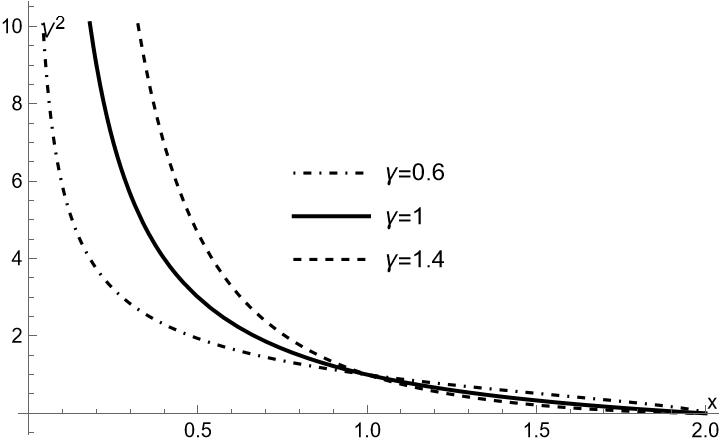
Figure 1: $V^{2}$ as function of $x$, for the three values of $\gamma$ indicated in the figure

In order to understand the results above, it is convenient to calculate the four–acceleration of a static observer in the frame of (10). We recall that a static observer is one whose four velocity $U^{\mu}$ is proportional to the Killing time–like vector Caroll , i.e.

$$U^{\mu}=\left[\frac{1}{(\frac{2m}{r}-1)^{\gamma/2}},0,0,0\right].$$ (40)

Then for the four–acceleration $a^{\mu}\equiv U^{\beta}U^{\mu}_{;\beta}$ we obtain for the region inner to the naked singularity

$$a^{\mu}=\left[0,-\frac{m\gamma\left(\frac{2m}{r}-1+\frac{m^{2}}{r^{2}}\sinh^{2}{\theta}\right)^{\gamma^{2}-1}}{r^{2}\left(\frac{2m}{r}-1\right)^{\gamma^{2}-\gamma}},0,0\right],$$ (41)

whereas for the region outside the naked singularity, described by (5) we obtain, with

$$U^{\mu}=\left[\frac{1}{(1-\frac{2m}{r})^{\gamma/2}},0,0,0\right],$$ (42)

$$a^{\mu}=\left[0,\frac{m\gamma\left(1-\frac{2m}{r}+\frac{m^{2}}{r^{2}}\sin^{2}{\theta}\right)^{\gamma^{2}-1}}{r^{2}\left(1-\frac{2m}{r}\right)^{\gamma^{2}-\gamma}},0,0\right].$$ (43)

The physical meaning of (41) and (43) is clear, it represents the inertial radial acceleration, which is necessary in order to maintain static the frame, by canceling the gravitational acceleration exerted on the frame, for the space–times (10) and (5) respectively. Since this acceleration is directed radially inwardly (outwardly), in the region inner (outer) to the naked singularity, it means that the gravitational force is repulsive (attractive). The attractive nature of gravitation in (5) is expected, whereas its repulsive nature in (10) is characteristic of hyperbolical space–times, and explains the peculiarities of the orbits inside the horizon. In particular, we see from (41) that the absolute value of the radial acceleration grows with $\gamma$, implying that the repulsion is stronger for larger $\gamma$, as it follows from the Figure 1.

We shall next consider the geodesics in the $\theta-r$ plane ($\phi=constant$). The interest of this case becomes intelligible if we recall that our space–time (10) is axially symmetric, implying that the general properties of motion on any slice $\phi=constant$ would be invariant with respect to rotation around the symmetry axis.

In this case, geodesic equations read

$$\ddot{t}-\frac{2\gamma m}{r^{2}(\frac{2m}{r}-1)}\dot{r}\dot{t}=0,$$ (44)

$$\ddot{r}-\frac{m\gamma(\frac{2m}{r}-1)^{2\gamma-\gamma^{2}}}{r^{2}(\frac{2m}{r}-1+\frac{m^{2}}{r^{2}}\sinh^{2}\theta)^{1-\gamma^{2}}}\dot{t}^{2}$$

$$-\frac{m}{r^{2}}\left[\frac{(\gamma^{2}-\gamma-1)}{\frac{2m}{r}-1}-\frac{(\gamma^{2}-1)\left(1+\frac{m}{r}\sinh^{2}{\theta}\right)}{\frac{2m}{r}-1+\frac{m^{2}}{r^{2}}\sinh^{2}{\theta}}\right]\dot{r}^{2}$$

$$-\frac{m^{2}(\gamma^{2}-1)\sinh 2\theta}{r^{2}\left(\frac{2m}{r}-1+\frac{m^{2}}{r^{2}}\sinh^{2}{\theta}\right)}\dot{\theta}\dot{r}+\left[r+m(\gamma^{2}-\gamma-2)\right.$$

$$\left.-\frac{m(\gamma^{2}-1)(1+\frac{m}{r}\sinh^{2}{\theta})\left(\frac{2m}{r}-1\right)}{\left(\frac{2m}{r}-1+\frac{m^{2}}{r^{2}}\sinh^{2}{\theta}\right)}\right]\dot{\theta}^{2}=0,$$

$$\ddot{\theta}+\frac{m^{2}(\gamma^{2}-1)\sinh 2\theta}{2r^{4}\left(\frac{2m}{r}-1\right)\left(\frac{2m}{r}-1+\frac{m^{2}}{r^{2}}\sinh^{2}{\theta}\right)}\dot{r}^{2}$$ (46)

$$+ 2\left[\frac{1}{r}+\frac{m(\gamma-\gamma^{2})}{r^{2}\left(\frac{2m}{r}-1\right)}+\frac{m(\gamma^{2}-1)\left(1+\frac{m}{r}\sinh^{2}{\theta}\right)}{r^{2}\left(\frac{2m}{r}-1+\frac{m^{2}}{r^{2}}\sinh^{2}{\theta}\right)}\right]\dot{\theta}\dot{r}$$

$$- \frac{m^{2}(\gamma^{2}-1)\sinh 2\theta}{2r^{2}\left(\frac{2m}{r}-1+\frac{m^{2}}{r^{2}}\sinh^{2}{\theta}\right)}\dot{\theta}^{2}=0.$$

To simplify the calculations we shall adopt a perturbative approach assuming $\gamma=1+\epsilon$, for $\epsilon<<1$, and neglecting terms of order $\epsilon^{2}$ and higher. Doing so we obtain from (46) at order $O(0)$ and $O(\epsilon)$ respectively

$$(\dot{\theta}r^{2}\dot{)}=0\quad\Rightarrow\quad\dot{\theta}=\frac{c_{1}}{r^{2}},$$ (47)

and

$$\frac{m^{2}\sinh 2\theta\,\dot{r}^{2}}{r^{4}(\frac{2m}{r}-1)(\frac{2m}{r}-1+\frac{m^{2}}{r^{2}}\sinh^{2}\theta)}$$

$$- \frac{m^{2}\sinh 2\theta\,\dot{\theta}^{2}}{r^{2}(\frac{2m}{r}-1+\frac{m^{2}}{r^{2}}\sinh^{2}\theta)}$$

$$- \frac{2m}{r^{2}}\left[\frac{1-\frac{2m}{r}+(\frac{2m}{r}-\frac{3m^{2}}{r^{2}})\sinh^{2}\theta}{(\frac{2m}{r}-1)(\frac{2m}{r}-1+\frac{m^{2}}{r^{2}}\sinh^{2}\theta)}\right]\dot{\theta}\,\dot{r}=0.$$

Introducing

$$\dot{r}=r_{\theta}\dot{\theta},\qquad y=\frac{m}{r},$$ (49)

equation (LABEL:dottheta1) becomes

$$y^{2}_{\theta}+\frac{2y_{\theta}}{\sinh 2\theta}\left[1-2y+(2y-3y^{2})\sinh^{2}\theta\right]-y^{2}(2y-1)=0,$$ (50)

whose integration produces

$$y=constant=1/2.$$ (51)

The order $O(0)$ can be easily calculated from (III) and (47), producing

$$\ddot{r}-\frac{mE^{2}}{r^{2}(\frac{2m}{r}-1)}+\frac{m\,\dot{r}^{2}}{r^{2}(\frac{2m}{r}-1)}+\frac{(r-2m)c_{1}^{2}}{r^{4}}=0,$$ (52)

whose first integral reads

$$\dot{r}=\sqrt{E^{2}-(\frac{2m}{r}-1)(\frac{c_{1}^{2}}{r^{2}}+1)},$$ (53)

or, introducing the variable $z$

$$\dot{r}=r_{\theta}\dot{\theta},\qquad z\equiv 2y=\frac{2m}{r},$$ (54)

$$z_{\theta}=\frac{1}{k}\sqrt{E^{2}-(z-1)(k^{2}z^{2}+1)},$$ (55)

with $c_{1}=-2mk$.

This equation was already obtained and solved for the case $\gamma=1$ (eq. (38) in 2nc ), with the boundary condition that all trajectories coincide at $\theta=0,z=1$. Here we present the integration of such an equation for the values indicated in the Figure 2 (please notice that we have used for this figure the variable $z=2y$ in order to keep the same notation for the order $O(0)$ as in 2nc ).

Let us now analyze in some detail the physical implications of Figure 2 and equation (51). As we see the solution of the order $0(\epsilon)$ maintains a constant value of $y$ which is the same value assumed in the boundary condition. At order $O(0)$ we see from Figure 2, that the particle never reaches the center, which may only happen as $k$ and $E$ tend to infinity. In either case the particle never crosses outwardly the surface $y=1/2$ ($z=1$), this happening only along the radial geodesic $\theta=0$. The influence of $\gamma$ in the final picture can be deduced by combining Figure 2 and equation (51).

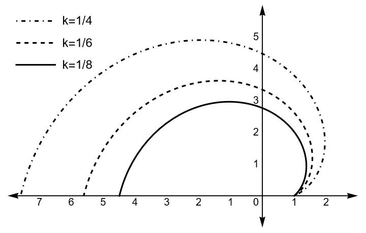
Figure 2: $z\equiv\frac{2m}{r}$ as function of $\theta$, for the values of $k$ indicated on the figure and $E=3$.

IV Conclusions

Motivated by the relevance of the $\gamma$-metric (5) and the hyperbolically symmetric metric (3), we have proposed in this work to analyze the physical properties of the hyperbolical version of the $\gamma$-metric. Such space–time described by the line element (10) shares with the hyperbolically symmetric space–time described by (3) some important features, the most relevant of which is the repulsive character of gravity inside the surface $r=2m$. On the other hand, as for the $\gamma$-metric (5), the surface $r=2m$ is not regular, thereby describing a naked singularity. The space–time (10) is not hyperbolically symmetric in the sense that it does not admit the Killing vectors (4), a fact suggesting the name “quasi–hyperbolically symmetric” for such space–time.

We have focused our study on the characteristics of the motion of test particles in the space–time described by (10), with special attention payed on the role of the parameter $\gamma$. Thus our main conclusions are:

1. Test particles may cross the surface $r=2m$ outwardly, but only along the axe $\theta=0$. This situation appears in the study of the geodesics in (3) presented in 2nc , however in our case the distinctive repulsive force of this space–time is increased by the parameter $\gamma$.

2. Like in the hyperbolically symmetric case, the test particles never reach the center, however in our case the test particles radially directed to the center bounce back farther from the center as $\gamma$ increases. This result becomes intelligible from a simple inspection of (41).

3. The motion of test particles on any slice $\phi=constant$ though qualitatively similar to the case $\gamma=1$, is affected by the value of $\gamma$ as follows from the analysis of Figure 2 and (51).

As we mentioned before, a new line of investigations based on observations of shadow images of the gravitationally collapsed aiming to the tests of gravity theories and corresponding black hole (or naked singularities) solutions for strong gravitational fields, is right now attracting the interest of many researchers. Such studies are particularly suitable for contrasting the physical relevance of different exact solutions to the field equations. We believe that the metric here exhibited deserves to be considered as a suitable candidate for such comparative studies. However it is worth mentioning that we have restricted our study to time–like geodesics, whereas any contrast with ETH observational data, would require results obtained from the study of null geodesics. Notwithstanding, the results obtained for time–like geodesics here presented, point to the potential of the metric under consideration.

We would like to conclude with a mention to what we believe is one of the most promising application of hyperbolical metrics. We have in mind the modeling of extragalactic relativistic jets. It should be clear that at present, such an application remains within the realm of speculation, however the comments below justify our (moderate) optimism.

Relativistic jets are highly energetic phenomena which have been observed in many systems (see Bladford ; Margon ; Sams ; blan and references therein), usually associated with the presence of a compact object, and exhibiting a high degree of collimation. Since no consensus has been reached until now, concerning the basic mechanism explaining these two features of jets (collimation and high energies), we feel motivated to speculate that the metric here considered could be considered as a possible engine behind the jets.

Indeed, on the one hand the collimation is ensured by the fact that test particles may cross the naked singularity outward, but only along the $\theta=0$ axis. On the other hand, as implied by (41), the strength of the repulsive gravitational force acting on the particle as $r\rightarrow 0$ increases as $\frac{1}{r^{(\gamma+2})}$. Explaining the high energies of particles bouncing back from regions close to $r=0$. More so, the fact that the repulsive force would be larger for larger values of $\gamma$, enhances further the efficiency of our model as the engine of such jets, as compared with the $\gamma=1$ case.

It goes without saying that the confirmation of this mechanism requires a much more detailed setup based on astronomical observations of jets, which is clearly out of the scope of this work.

- (1) Herrera, L; Witten, L. An alternative approach to the static spherically symmetric vacuum global solutions to the Einstein’s equations. Adv. High Ener. Phys. 2018, 2018, 3839103 .
- (2) Rosen, N. The nature of the Schwarzschild singularity. In Relativity; Carmeli, M., Fickler, S. I., Witten, L. Eds.; Plenum Press: New York, USA, 1970; pp.229–258.
- (3) Caroll, S. Spacetime and Geometry. An Introduction to General Relativity, Addison Wesley: San Francisco, USA, 2004; pp. 246.
- (4) Rindler, W. Relativity. Special, General and Cosmological, Oxford University Press: New York, USA, 2001; pp. 260–261.
- (5) Harrison, B. K. Exact Three–Variable Solutions of the Field Equations of General Relativity. Phys. Rev. 1959, 116, 1285.
- (6) Ellis, G. Dynamics of Pressure–Free Matter in General Relativity. J. Math. Phys. 1967, 8, 1171.
- (7) Stephani, H.; Kramer, D.; MacCallum, M.; Honselaers, C.; Herlt, E. Exact Solutions to Einsteins Field Equations, 2nd ed.; Cambridge University Press: Cambridge, England 2003.
- (8) Gaudin, M.; Gorini, V.; Kamenshchik, A.; Moschella, U.; Pasquier, V. Gravity of a static massless scalar field and a limiting Schwarzschild-like geometry. Int. J. Mod. Phys. D 2006, 15, 1387–1399.
- (9) Rizzi, L.; Cacciatori, S.L.; Gorini, V.; Kamenshchik, A.; Piattella, O.F. Dark matter effects in vacuum spacetime. Phys. Rev. D 2010, 82, 027301.
- (10) Kamenshchik, A.Y.; Pozdeeva, E.O.; Starobinsky, A.A.; Tronconi, A.; Vardanyan, T.; Venturi, G.; Yu, S. Verno. Duality between static spherically or hyperbolically symmetric solutions and cosmological solutions in scalar-tensor gravity. Phys. Rev. D 2018, 98, 124028.
- (11) Madler, T. On the affine-null metric formulation of General Relativity. Phys. Rev. D 2019, 99, 104048.
- (12) Maciel, A.; Delliou, M.L.; Mimoso, J.P. New perspectives on the TOV equilibrium from a dual null approach. Class. Quantum Gravity 2020, 37,125005.
- (13) Herrera, L; Di Prisco, A; Ospino, J; Witten, L. Geodesics of the hyperbolically symmetric black hole. Phys. Rev. D 2020, 101, 064071.
- (14) Bhatti, M. Z.; Yousaf, Z.; Tariq,Z. Hyperbolically symmetric sources in Palatini gravity Eur. Phys. J. C 2021, 81, 1070.
- (15) Herrera, L; Di Prisco, A; Ospino, J. Dynamics of hyperbolically symmetric fluids. Symmetry 2021, 13, 1568.
- (16) Herrera, L; Di Prisco, A; Ospino. J. Hyperbolically symmetric static fluids: A general study. Phys. Rev. D 2021 103, 024037.
- (17) Herrera, L.; Di Prisco, A.; Ospino, J. Hyperbolically symmetric versions of Lemaitre–Tolman–Bondi spacetimes. Entropy 2021, 23, 1219.
- (18) Bhatti, M.Z.; Yousaf , Z.; Tariq, Z. Influence of electromagnetic field on hyperbolically symmetric source. Eur. Phys. J. P. 2021, 136, 857.
- (19) Bhatti, M. Z.; Yousaf, Z.; Hanif, S. Hyperbolically symmetric sources, a comprehensive study in gravity. Eur. Phys. J. P. 2022, 137, 65.
- (20) Lim, Y. Motion of charged particles in spacetimes with magnetic fields of spherical and hyperbolic symmetry. Phys. Rev. D 2022, 106, 064023.
- (21) Yousaf, Z.; Bhatti, M.; Khlopov, M.; Asad, H. A Comprehensive Analysis of Hyperbolical Fluids in Modified Gravity. Entropy 2022, 24, 150.
- (22) Yousaf, Z.; Bhatti, M.; Asad, H. Hyperbolically symmetric sources in gravity. Ann. Phys. 2022, 437, 168753.
- (23) Yousaf, Z.; Nashed, G.; Bhatti , M., Asad, H. Significance of Charge on the Dynamics of Hyperbolically Distributed Fluids. Universe 2022, 8, 337.
- (24) Yousaf, Z. Spatially Hyperbolic Gravitating Sources in -Dominated Era Universe 2022, 8, 131.
- (25) Bhatti, M. Z.; Yousaf, Z.; Hanif. S. Electromagnetic influence on hyperbolically symmetric sources in gravity. Eur. Phys. J. C 2022, 82, 340.
- (26) Zipoy, D.M. Topology of Some Spheroidal Metrics. J. Math. Phys. 1966, 7, 1137-1143.
- (27) Vorhees B. Static Axially Symmetric Gravitational Fields. Phys. Rev. D 1970, 2, 2119.
- (28) Espósito, F.; Witten, L. On a static axisymmetric solution of the Einstein equations. Phys. Lett. B 1975, 58, 357-360.
- (29) Duncan, C.; Esposito, F.; Lee, S. Effects of naked singularities: Particle orbits near a two-parameter family of naked singularity solutions. Phys. Rev. D 1978, 17, 404.
- (30) Herrera, L.; Paiva, F.; Santos, N.O. Geodesics in the spacetime. Int. J. Mod. Phys. D 2000, 9, 49.
- (31) W. B. Bonnor, Proceedings of the 3rd Canadian Conference on General Relativity and Relativistic Astrophysics eds. A. Coley, F. I.Cooperstock and B. Tupper (World Scientific Publishing Co., Singapore, 1990) p. 216.
- (32) Herrera, L.; Paiva , F. M.; Santos, N. O. The Levi-Civita spacetime as a limiting case of the spacetime. J. Math. Phys. 1999, 40, 4064-4071.
- (33) Richterek, L.; Novotny, J.; Horsky, J. Einstein-Maxwell Fields Generated from the Metric and Their Limits. Czech. J. Phys. 202, 52, 1021-1040.
- (34) Chowdhury, A.; Patil, M; Malafarina, D.; Joshi, P. Circular geodesics and accretion disks in the Janis-Newman-Winicour and gamma metric spacetimes. Phys. Rev. D 2012, 85, 104031.
- (35) Abdikamalov, A.; Abdujabbarov, A.; Ayzenberg, D.; Malafarina, D.; Bambi, C.; Ahmedov. B. Black hole mimicker hiding in the shadow: Optical properties of the metric. Phys. Rev. D 2019, 100, 024014.
- (36) Alvear Terrero, D.; Hernandez Mederos, V.; Lopez Perez, S.; Manreza Paret, D.; Perez Martinez, A.; Quintero Angulo, G. Modeling anisotropic magnetized white dwarfs with metric. Phys. Rev. D 2019, 99, 02301
- (37) Toshmatov, B.; Malafarina, D.; Dadhich, N. Harmonic oscillations of neutral particles in the metric. Phys. Rev.D 2019, 100, 044001.
- (38) Toshmatov, B.; Malafarina, D. Spinning test particles in the spacetime. Phys. Rev. D 2019, 100, 104052.
- (39) Benavides Gallego, C.; Abdujabbarov, A.; Malafarina, D.; Ahmedov, B.; Bambi, C. Charged particle motion and electromagnetic field in spacetime. Phys. Rev. D 2019, 99, 044012.
- (40) Capistrano, A.; Zeidel, P.; Cabral, L. Effective apsidal precession from a monopole solution in a Zipoy spacetime Eur. Phys. J. C 2019, 79, 730.
- (41) Benavides Gallego, C.; Abdujabbarov, A.; Malafarina, D.; Bambi, C. Quasiharmonic oscillations of charged particles in static axially symmetric space-times immersed in a uniform magnetic field. Phys. Rev. D 2020, 101, 124024.
- (42) Narziloev, B.; Malafarina, D.; Abdujabbaraov, A.; Bambi, C. On the properties of a deformed extension of the NUT space-time. Eur. Phys. J. C 2020, 80, 784.
- (43) Ai-Rong Hu; Guo-Qing Huang, Dynamics of charged particles in the magnetized space–time. Eur. Phys. J. P. 2021, 136, 1210.
- (44) Turimov, B.; Ahmedov, B. Zipoy-Voorhees Gravitational Object as a Source of High-Energy Relativistic Particles. Galaxies 2021, 9, 59.
- (45) Malafarina, D.; Sagynbayeva, S. What a difference a quadrupole makes? Gen. Relativ. Gravit. 2021, 53, 112.
- (46) Memmen, J.; Perlick, V. Geometrically thick tori around compact objects with a quadrupole moment. Class. Quantum Gravit. 2021, 38, 135002.
- (47) Narzilloev, B.; Malafarina, D.; Abdujabbarov, A.; Ahmedov, B.; Bambi, C. Particle motion around a static axially symmetric wormhole. Phys. Rev. D 2021, 104, 064016.
- (48) Chakrabarty, H.; Borah, D.; Abdujabbarov, A.; Malafarina, D.; Ahmedov, B. Effects of gravitational lensing on neutrino oscillation in spacetime. Eur. Phys. J. C 2022, 82. 24.
- (49) Ajibarat, A.; Mirza, B.; Azizallahi, A. Metrics in higher dimensions. Nucl. Phys. B 2022, 978, 115739.
- (50) Shaikh, R.; Paul, S.; Banerjejee, P.; Sarkar, T. Shadows and thin accretion disk images of the -metric. Eur. Phys. J. C 2022, 82, 696.
- (51) Gurtug, O.; Halilsoy, M.; Mangut, M. The charged Zipoy-Voorhees metric with astrophysical applications. Eur. Phys. J. C 2022, 82, 671.
- (52) Li, S.; Mirzaev, T.; Abdujabbarov, A.; Malafarina, D.; Ahmedov, B.; Wen-Biao Han, Constraining the deformation of a rotating black hole mimicker from its shadow. Phys. Rev. D 2022, 106, 08041.
- (53) Akiyama, K. et al. (Event Horizon Telescope Collaboration). First M87 Event Horizon Telescope Results. I. The Shadow of the Supermassive Black Hole. Astrophys. J. Lett. 2019, 875, L1.
- (54) Akiyama, K. et al. (Event Horizon Telescope Collaboration). First Sagittarius A Event Horizon Telescope Results. I. The Shadow of the Supermassive Black Hole in the Center of the Milky Way. Astrophys. J. Lett. 2022, 930, L12.
- (55) Psaltis, D. Testing general relativity with the Event Horizon Telescope. Gen. Relativ. Gravit. 2019, 51, 137.
- (56) Gralla, S. E. Can the EHT M87 results be used to test general relativity?. Phys. Rev. D 2021, 103, 024023.
- (57) Glampedakis, K.; Pappas, G. Can supermassive black hole shadows test the Kerr metric?. Phys. Rev. D 021, 104, L081503.
- (58) Ghasemi–Nodehi, M.; Azreg–Ainou, M.; Jusufi, K.; Jamil, M. Shadow, quasinormal modes, and quasiperiodic oscillations of rotating Kaluza-Klein black holes. Phys. Rev. D 2020, 102, 104032.
- (59) Jusufi, K.; Azreg–Ainou, M.; Jamil, M.; Wei, S.W.; Wu, Q.; Wang, A. Quasinormal modes, quasiperiodic oscillations, and the shadow of rotating regular black holes in nonminimally coupled Einstein-Yang-Mills theory. Phys. Rev. D 2021, 103, 024013.
- (60) Liu, C.; Zhu, T.; Wu, Q.; Jusufi, K.; Jamil, M.; Azreg–Ainou, M.; Wang, A. Shadow and quasinormal modes of a rotating loop quantum black hole. Phys. Rev. D 2020, 101, 084001.
- (61) Jusufi, K.; Jamil, M.; Chakrabarty, H.; Wu, Q.; Bambi, C.; Wang, A. Rotating regular black holes in conformal massive gravity. Phys. Rev. D 101 2020, 044035.
- (62) Afrin, M.; Kumar, R.; Ghosh, S.G. Parameter estimation of hairy Kerr black holes from its shadow and constraints from M87. Mon. Not. R. Astron. Soc. 2021, 504, 5927.
- (63) Volkov, M.S. Self-accelerating cosmologies and hairy black holes in ghost-free bigravity and massive gravity. Classical Quantum Gravity 2013, 30, 184009.
- (64) Benkel, R.; Sotiriou, T. P.; Witek, H. Black hole hair formation in shift-symmetric generalised scalar-tensor gravity. Classical Quantum Gravity 2017, 34, 064001.
- (65) Cardoso, V.; Gualtieri, L. Testing the black hole “no-hair” hypothesis. Classical Quantum Gravity 2016, 33, 174001.
- (66) Kurmanov, E.; Boshkayev, K.; Giambo, R.; Konysbayev, T.; Luongo, O.; Malafarina, D.; Quevedo, H. Accretion Disk Luminosity for Black Holes Surrounded by Dark Matter with Anisotropic Pressure. Astrophys. J. 2022, 925, 210.
- (67) Boshkayev, K.; Konysbayev, T.; Kurmanov, E.; Luongo, O.; Malafarina, D.; Mutalipova, K.; Zhumakhanova, G. Effects of non-vanishing dark matter pressure in the Milky Way Galaxy. Mon. Not. R. Astron. Soc. 2021, 508, 1543.
- (68) Boshkayev, K.; Idrissov, A.; Luongo, O.; Malafarina, D. Accretion disc luminosity for black holes surrounded by dark matter. Mon. Not. R. Astron. Soc. 2020, 496, 1115.
- (69) Israel, W. Event Horizons in Static Vacuum Space-Times Phys. Rev. 1967, 164, 1776.
- (70) Blandford, R. D.; Rees, M. J. A “Twin-Exhaust?? Model for Double Radio SourcesMon. Not. R. Astron. Soc. 1974, 169, 395.
- (71) Margon, B. A. Observations of SS 433. Annu. Rev. Astr. Astrophys 1984, 22, 507.
- (72) Sams, B. J. ; Eckart , A.; Sunyaev, R. Near-infrared jets in the Galactic microquasar . Nature 1996, 382, 47-49.
- (73) Blandford, R. D. AGN Jets . Astr. Soc. Pacif. Conf. Ser. 2003, 290, 267.