Gravitational waves from Axion wave production.

Abstract

We consider a scenario with axions/axion-like particles Chern-Simons gravity coupling, such that gravitational waves can be produced directly from axion wave tachyonic instability in the early universe after inflation. This axion gravity term is less constrained compared to the well-searched axion photon coupling and can provide a direct and efficient production channel for gravitational waves. Such stochastic gravitational waves can be detected by either space/ground-based gravitational wave detectors or pulsar timing arrays for a broad range of axion masses and decay constants.

I Introduction

Since the first observation of gravitational waves (GWs), we have acquired a new way to probe the current and early universe and it has a great impact on the fields of astrophysics, cosmology, and even particle physics. Gravitational waves at different frequencies from various sources are from the primordial gravitational waves at $10^{-16}$ HzTurner:1996ck ; Smith:2005mm ; Caprini:2018mtu , NanoHz$10^{-9}$ HzNANOGrav:2023hvm ; Li:2023yaj ; Kitajima:2023vre ; NANOGrav:2023bts ; Kitajima:2023cek to the binary system signals up to $10^{4}$ Hz. This whole spectrum of gravitational waves need different detection scheme, from CMB polarization, Pulsar timing arrayManchester_2013 ; Ferdman_2010 ; jenet2009north ; Hobbs_2010 ; Manchester_2013_1 ; Xu:2023wog , interferometryAudley:2017drz ; Cornish:2018dyw ; Luo:2015ght ; Guo:2018npi ; Gong:2014mca ; Coleman:2018ozp ; Corbin:2005ny ; Musha:2017usi ; Punturo:2010zz ; Evans:2016mbw ; LIGOScientific:2007fwp ; LIGOScientific:2014pky ; VIRGO:2014yos , as well as some high-frequency proposals Aggarwal:2020olq ; Gottardi:2007zn ; Aguiar:2010kn ; Akutsu:2008qv ; Nishizawa:2007tn ; Ejlli:2019bqj ; Cruise_2006 ; Goryachev:2014yra .

Around one-fourth of the universe’s total energy budget is made of dark matter from cosmological and astronomical observations. Aside from the well-searched weakly interacting massive particles (WIMPs), axion 1983Cosmology ; Visinelli:2009kt ; Panci:2022wlc ; Adams:2022pbo ; Co:2017mop is a promising dark matter candidate, as well as a natural solution to the ‘Strong CP problem’ Michael1981A ; Hook:2018dlk in quantum chromodynamics (QCD)Skands:2012ts . The axion was proposed as the Nambu-Goldstone boson of the spontaneously broken global U(1)PQ symmetry extension of the Standard Model (SM). When the universe cools down to the QCD scale the axion acquires a tiny mass and becomes a pseudo-Nambu-Goldstone particle. After the QCD phase transition, the axion field begins to oscillate and the energy density from classical oscillation can play the role of dark matterCo:2017mop . In well-motivated scenarios such as the Dine-Fischler-Srednicki-Zhitnitsky (DFSZ) PhysRevD.107.095020 ; Zhitnitskij1980OnPS ; Michael1981A and the Kim-Shifman-Vainshtein-Zakharov (KSVZ) PhysRevLett.43.103 ; SHIFMAN1980493 models, QCD axions’s characteristic axion-gluon coupling is generated via SU(3)c-charged fermion loops. In general axion-like particles (ALPs) are light bosons that have electromagnetic Chern-Simons (CS) type of coupling but are not necessarily coupled to gluons. ALPs can also acquire axion-graviton Chern-Simons coupling, which can be generated through heavy particle loops. The axion-graviton coupling can also induce axion photon coupling with Planck suppression Sun:2020gem . ALPs are abundant in string-theory motivated models Svrcek:2006yi ; Marchesano:2014mla ; ALPs generally can have a much wider mass range as the dark matter candidate. We will use ‘axion’ to denote both the QCD axion and ALPs.

The gravitational wave from axion was considered with the axion dark gauge boson coupling, to avoid the stringent constraints from axion photon couplings. For the inflationary scenario that axion is the inflaton, axion gauge boson coupling can induce large primordial gravitational waves e.g. in the so-called axion monodromy model through tachyonic instability McAllister:2008hb ; DiLuzio:2020wdo ; Hebecker:2016vbl ; Anber:2009ua ; Barnaby:2012xt ; Anber:2012du ; Domcke:2016bkh . If considering the mechanism that axion oscillates after inflation, tachyonic instability in a dark gauge field induced by an axion-like particle is a known source of dark matter and/or stochastic gravitational wavesMadge:2021abk ; Machado:2018nqk ; Machado:2019xuc ; Kitajima:2020rpm ; Geller:2023shn ; Dror:2018pdh ; Co:2018lka ; Bastero-Gil:2018uel ; Agrawal:2018vin , and friction for relaxionHook:2016mqo ; Fonseca:2018xzp .

Here in this paper, we consider a less studied axion graviton Chern-Simons coupling in the early universe after inflation, such that this term can produce gravitational waves directly through axion rolling tachyonic instability. The effect of such coupling term has been studied in inflationary scenarios for primordial gravitational wave production, and binary merger of black holes Alexander:2009tp . However, for high-scale inflationary scenarios, the ghost issues in Chern-Simons gravity may become severe. In this work, the frequency of directly produced gravitational waves is $10^{-9}\mathrm{Hz}\sim 10^{-2}\mathrm{Hz}$. Due to the large parameter space of axion mass, we can possibly observe such gravitational wave spectrum as low as PTA bandManchester_2013 ; Ferdman_2010 ; jenet2009north ; Hobbs_2010 ; Manchester_2013_1 when $m_{a}\sim 10^{-12}$eV, up to space interferometry 0.01 Hz Audley:2017drz ; Cornish:2018dyw ; Luo:2015ght ; Guo:2018npi when $m_{a}\sim 1$eV. The gravitational wave spectrum here has a peak frequency and is spread out around one order of magnitude by the universe expansion.

This paper is organized as follows. In section II we briefly review the axion evolution equations in the early universe with axion graviton Chern-Simons coupling and universe expansion. We study how the axions produce GWs in section III. In section IV, we summarize and discuss our result.

II Model

We begin with the action of Chern-Simons modified gravity with axion coupling:

$$S=\int d^{4}x\sqrt{-g}\left(\frac{R}{16\pi G}+\frac{\alpha}{4}\phi R\tilde{R}+\frac{1}{2}\partial_{\mu}\phi\partial^{\mu}\phi-V(\phi)\right)$$ (1)

where $R$ is the Ricci scalar, $R\tilde{R}=\frac{1}{2}\epsilon^{\rho\sigma\alpha\beta}R^{\mu\nu}_{\alpha\beta}R_{\nu\mu\rho\sigma}$, and the potential of axion field is

$$V(\phi)=m_{a}^{2}f^{2}\left[1-\cos\left(\frac{\phi}{f}\right)\right],$$ (2)

where $m_{a}$ is the mass of axions. If neglecting the backreaction of gravitational waves, the equation of motion of the axion field is Machado:2018nqk

$$\ddot{\frac{\phi}{f}}+3H\dot{\frac{\phi}{f}}+m_{a}^{2}\sin\frac{\phi}{f}=0$$ (3)

While the Hubble parameter $H\gg m_{a}$, $\phi$ remains constant. When the universe cools down to $H\approx m_{a}$, the axion field begins rolling toward the minimum of the potential and then oscillates. Assuming a radiation-dominated universe, the temperature when $H=m_{a}$ is

$$T_{*} =\left(\frac{45}{4\pi^{3}}\right)^{1/4}g_{*}^{-1/4}m_{a}^{1/2}G^{-1/4}$$ (4)

$$=2.7118\times 10^{4}\left(\frac{g_{*}}{100}\right)^{-1/4}\left(\frac{m_{a}}{\mathrm{eV}}\right)^{1/2}\mathrm{GeV}$$

for a wide range of axion mass, i.e., $m_{a}\in[10^{-12}\mathrm{eV},1\mathrm{eV}]$, the radiation dominated assumption is consistent Machado:2018nqk . In the following study, to solve Eq.(3), we chose initial conditions $\phi(t_{*})/f=\theta\sim\mathcal{O}(1),\dot{\phi}(t_{*})=0,H(t_{*})=m_{a}$.

We consider a Friedmann-Robertson-Walker (FRW) Universe. The perturbed metric reads

$$ds^{2}=-dt^{2}+a^{2}(t)\left(\delta_{ij}+h_{ij}(t,\mathbf{x})\right)dx^{i}dx^{j},$$ (5)

where the scale factor $a=\sqrt{t/t_{*}}=\sqrt{2tm_{a}}$ for radiation dominated Universe. We have chosen $a(t_{*})=1$ in the whole study. In Fourier space

$$h_{ij}(t,\mathbf{x})=\sum_{A=R,L}\int\frac{d^{3}k}{(2\pi)^{3}}h_{A}(t,k)e^{i\vec{k}\cdot\vec{x}}e_{ij}^{A}$$ (6)

where $A=L,R$ labels the left-handed and right-handed polarization, respectively. The equations of motion for $h_{A}$ can be derived from the actionChu:2020iil ,

$$\ddot{h}_{A}+\left(3H+\frac{\dot{D}_{A}}{D_{A}}\right)\dot{h}_{A}+\frac{k^{2}}{a^{2}}h_{A} =0,$$ (7)

$$\mathrm{with}\quad D_{A}=1-\frac{\lambda_{A}k}{am_{cs}},\quad\lambda_{L}=-1,\lambda_{R} =1,m_{cs}=(16\pi G\alpha\dot{\phi})^{-1}$$

For $\frac{k}{a}>|m_{cs}|$, $1/D_{A}$ diverges, which indicates that there are ghost modesDyda:2012rj . In our study of the resonant amplification of GWs, to avoid the ghost modes, we take the regulator:

$$\frac{k}{am_{cs}}\longrightarrow\frac{k}{am_{cs}}f\left(\frac{k}{a\Lambda}\right),\mathrm{with}\quad f(x)=\begin{cases}0,&x>1,\\ 1,&x<1.\end{cases}$$ (8)

For $t\gg t_{0}$, we numerically solve for $\dot{\phi}\sim\theta fA_{1}m_{a}a(t)^{-3/2}\sin(m_{a}t+\psi_{0})$. And then we chose $\Lambda=\left(16\pi G\alpha a(t)^{-3/2}\theta f\left(A_{1}m_{a}+\frac{A_{2}}{t}\right)\right)^{-1}$, where $A_{1}=1.66415,A_{2}=-0.118543$ are numerically determined by requiring the cut-off scale to be less than the amplitude of the oscillating $m_{cs}$, $|m_{cs}|\geq\Lambda$. For physical wavenumber $k/a<\Lambda$, the equations of motion are almost unchanged. For $k/a>\Lambda$, the regulator is equivalent to turning off the CS term for simplicity. Technically we use $f(x)=(1+x^{20})^{-1}$.

From the viewpoint that the model is an effective quantum field theory, for $k/a>\Lambda$, the ghost appears and physics from higher-order terms should be considered. Fig.1 shows where ghost modes appear in the blue region corresponding to $k/a>|m_{cs}|$. Notice here $m_{cs}$ oscillates with axion $\dot{\phi}$. We have chosen $\theta=1,\alpha fm_{a}^{2}=5\times 10^{37}\mathrm{GeV}^{2}$.

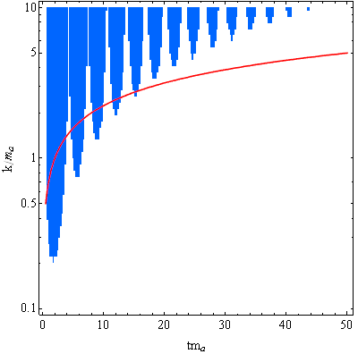
Figure 1: The blue region corresponds to $k/a>|m_{cs}|$, and the red line is $k/a=m_{a}/2$ where the resonance occurs, as we will discuss in the next section.

III Resonant amplification of GWs

The enhancement of GWs passing through the axion cloud has been studied in Sun:2020gem ; Yoshida:2017cjl ; Chu:2020iil ; Lambiase:2022ucu . Those studies mainly focus on a much later epoch when $H\ll m_{a}$ and the universe expansion effects can be neglected. Their result shows that a resonant amplification of GWs happens when $k=m_{a}/2$. However, when considering the Universe’s expansion, it becomes slightly different. Fig.III shows how the amplitudes of GWs evolve for $k=10m_{a}$ as an exemplifying mode value $k/a$. $h_{A}/h_{0}$ is the amplitude of GWs normalized by the initial value. When $k/a\gg m_{a}$, the amplitudes are almost unchanged. As time went by, $k/a$ decreased. When $k/a\sim m_{a}/2$, resonant amplification occurs, and $h_{L}$ increases exponentially. Notice that in our calculation the two modes evolve dramatically differently, which implies that the CS-modified gravity breaks the parity symmetry. Notice that making replacement $\phi\rightarrow-\phi,L\leftrightarrow R$ do not change Eq.7, which means that two modes behaviors switch if we use a different initial conditions $\phi(t_{*})=-f\theta$. When $a$ becomes sufficiently large, $k/a$ becomes much smaller than $m_{a}/2$, resonant amplification stops and $h_{A}$ decreases slowly as the Universe expands.

evolution of $h_{A}$ when $k=10m_{a}$. For left plot, we have chose $\theta=1,\alpha fm_{a}^{2}=5\times 10^{37}\mathrm{GeV}^{2}$, while for right plot $\alpha fm_{a}^{2}=2.5\times 10^{37}\mathrm{GeV}^{2}$.

For different values $k/m_{a}$, we numerically solve Eq.(7) and obtain magnification of GWs. The energy density $\Omega\propto h_{A}^{2}$. When $a\gg 2k/m_{a}$, $\Omega/\Omega_{0}$ trends to a constant, where $\Omega_{0}$ is the energy density when CS modification is absent. The results are shown in Fig.2. For $k\gg m_{a}$, the axion field $\phi$ becomes much smaller when $k/a=m_{a}/2$, thus the magnifications are small. For $k<5m_{a}$, $k/a$ varies too fast when resonant amplification happens, which leads to less time for resonant amplification. The peak of GWs is at $k\sim 6m_{a}$ for parameters $\theta=1,\alpha fm_{a}^{2}=5\times 10^{37}\mathrm{GeV}^{2}$. As Fig.1 shows, for $k<3m_{a}$, $\left|\frac{k}{am_{cs}}\right|>1$ when $k/a=m_{a}/2$, where we turned on our regulator.

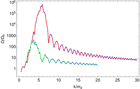
Figure 2: Magnification of energy density for GWs. Red line corresponding to $\theta=1,\alpha fm_{a}^{2}=5\times 10^{37}\mathrm{GeV}^{2}$, while green line corresponding to $\alpha fm_{a}^{2}=2.5\times 10^{37}\mathrm{GeV}^{2}$.

Inflation can generate a scale-invariant gravitational wave spectrum. The spectrum can be approximated bySaikawa:2018rcs

$$\Omega_{\mathrm{gw}}h^{2}(\tau_{0},k) \approx\frac{1}{24}\Omega_{\gamma}h^{2}\left(\frac{g_{\star\rho,\mathrm{hc}}}{2}\right)\left(\frac{g_{\star s,\mathrm{hc}}}{g_{\star s,\mathrm{fin}}}\right)^{-\frac{4}{3}}\mathcal{P}_{T}(k)$$ (9)

$$\approx 1.29\times 10^{-17}\left(\frac{g_{*s,\mathrm{fin}}}{3.931}\right)^{\frac{4}{3}}\left(\frac{g_{*s,\mathrm{hc}}}{106.75}\right)\left(\frac{g_{*s,\mathrm{hc}}}{106.75}\right)^{-\frac{4}{3}}\left(\frac{V_{\mathrm{inf}}^{1/4}}{10^{16}\,\mathrm{GeV}}\right)^{4},$$

where $V_{\mathrm{inf}}^{1/4}$ is the energy scale of inflation. If there exist axions, the GWs from inflation can be magnified at certain specific frequencies. We can also consider the other sources as the seeds for the stochastic gravitational waves for our axion enhancement study. Here for simplicity, we just take the simplest scale invariant spectrum from inflation as an example. Suppose GWs induced by inflation is about $h^{2}\Omega_{0}\sim 10^{-16}$Saikawa:2018rcs , which is well below the upper bound on the amount of radiation $\int\Omega_{GW}(k)d\ln k\leq 5.6\times 10^{-6}\Delta N_{eff}$ Aggarwal:2020olq , where $\Delta N_{eff}$ is the extra neutrino species and roughly satisfes the condition $\Delta N_{eff}<0.2$. We show the energy density after the amplification by axions in Fig.3. The energy density shape depends on the magnification of Fig.2 and the frequencies are

$$f =\frac{k}{2\pi}\frac{a_{*}}{a_{0}}=\frac{k}{2\pi}\frac{T_{0}}{T_{*}}\left(\frac{g_{0}}{g_{*}}\right)^{1/3}$$ (10)

$$\approx 7.125\times 10^{-4}\left(\frac{100}{g_{*}}\right)^{1/12}\left(\frac{k}{m_{a}}\right)\left(\frac{m_{a}}{\mathrm{eV}}\right)^{1/2}\mathrm{Hz}.$$

We have used Eq.4 and $T_{0}=2.725\mathrm{K},g_{0}=3.938$. The value $k/m_{a}$ can be directly taken from Fig.2. The parameters for Fig.3 are shown in table 1, where BP3 and BP4 are consistent with the QCD axion.

The frame-dragging experiments gives a limit for CS gravity coupling bySmith:2007jm ; Alexander:2009tp $\kappa^{-1}\alpha\dot{\phi}<3000\mathrm{km}$, or $\alpha\Omega_{\phi}^{1/2}<5.25\times 10^{81}\mathrm{GeV}^{-1}$, where $\Omega_{\phi}$ is energy fractions of axions nowadays. The energy fraction of axions when the axion field began to oscillate is $\Omega_{\phi}\sim 2.6\times 10^{-4}\left(\frac{f}{10^{17}\mathrm{GeV}}\right)^{2}$, which is consistent with the radiation dominated universe. Energy fractions of GWs at $H=m_{a}$ is $\Omega_{gw*}\simeq 2.78\times 10^{4}\left(\frac{g_{*}}{100}\right)^{1/3}\Omega_{gw}(T=2.7K)$. For $\Omega_{gw}(T=2.7K)\sim 10^{-10}$, energy density when $H=m_{a}$ is about $\Omega_{gw*}\sim 10^{-6}$. In our calculations, $\int\Omega_{gw*}(f)d\ln(f)\ll\Omega_{\phi}$ is always maintained, thus we can safely neglect the back reaction from GWs to axion dynamics.

When $H\ll m_{a},\ddot{a}/a\ll m_{a}^{2}$, Eq.(3) has a solution $\phi(t)\approx\phi(t_{i})(a/a_{i})^{-3/2}\cos\left(m(t-t_{i})\right)$, thus the energy density $\rho_{\phi}\propto a^{-3}$, which behaves like the dark matter. To avoid the redundant dark matter, $\phi$ should decay to other particles such as dark photonsMachado:2018nqk . In our scenario, the axion decay width should fulfill $\Gamma\ll m_{a}$ to generate GWs before decaying.

In Fig.3, the dashed part of each line denotes the region $\left|\frac{k}{am_{cs}}\right|>1$ when $k/a=m_{a}/2$ and our regulator is turned on, thus our result may be unreliable in these regions. We find that, after the axion enhancement, the GWs can be possibly detected by TaijiGuo:2018npi , TianQinLuo:2015ght , LISAAudley:2017drz for axion mass $m_{a}=10^{-3}\mathrm{eV}\sim 1\mathrm{eV}$ and can be detected by IPTAHobbs_2010 , SKA5136190 ; Moore:2014lga for $m_{a}=10^{-12}\mathrm{eV}$.

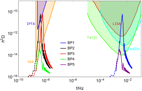
Figure 3: GWs spectra after the amplification by axions. The dashed part of each line denotes the region $\left|\frac{k}{am_{cs}}\right|>1$ when $k/a=m_{a}/2$ and our regulator is turned on. We plot 5 benchmark points with the parameters in Table 1. We show the sensitivity curves from TaijiGuo:2018npi , TianQinLuo:2015ght , LISAAudley:2017drz as well as IPTAHobbs_2010 , SKA5136190 ; Moore:2014lga .

–	$m_{a}$	$f$	$\alpha$	$\theta$
BP1(ALP)	$1\mathrm{eV}$	$10^{17}\mathrm{GeV}$	$5\times 10^{38}\mathrm{GeV}^{-1}$	1
BP2(ALP)	$10^{-12}\mathrm{eV}$	$10^{17}\mathrm{GeV}$	$5\times 10^{62}\mathrm{GeV}^{-1}$	1
BP3(QCD axion)	$2\times 10^{-12}\mathrm{eV}$	$3\times 10^{18}\mathrm{GeV}$	$4.2\times 10^{60}\mathrm{GeV}^{-1}$	1
BP4(QCD axion)	$2\times 10^{-12}\mathrm{eV}$	$3\times 10^{18}\mathrm{GeV}$	$2.1\times 10^{60}\mathrm{GeV}^{-1}$	1
BP5(ALP)	$1\mathrm{eV}$	$10^{16}\mathrm{GeV}$	$2.5\times 10^{39}\mathrm{GeV}^{-1}$	1

Table 1: Parameters for 5 benchmark point in Fig.3. Notice that BP3 and BP4 are consistent with the QCD axion.

IV discussion and summary

We propose a novel generation mechanism for gravitational waves, as well as an efficient way to detect axions/ALPs. The tachyonic instability in the axion-graviton coupling is a less studied effect previously, and not much constrained compared to the axion-photon coupling. The Chern-Simons axion-graviton coupling is an interesting modification to Einstein gravity, an extension of the effective field theory of Einstein-Hilbert action. This Chern-Simons gravity term can generate axion-photon coupling at the loop level with Planck suppression. The large coupling of axion-graviton can generate gravitational waves in a radiation-dominated era, much later than inflation and preheating time which people usually explored.

The peak frequency of the generated GWs is red-shifted today and can be detected by different GW detection methods, from $10^{-9}$Hz up to $10^{-2}$Hz. We have also numerically studied the shape of the GW spectrum, without considering the backreaction, which can be a future direction. The upper bounds of this power spectrum are mostly from observation, as we discussed earlier. The parameters we used in the figure are well below the bounds from $\Delta N_{eff}$ in the radiation era, so this mechanism can be a source for large dark radiation.

- [1] Michael S. Turner. Detectability of inflation produced gravitational waves. Phys. Rev. D, 55:R435–R439, 1997.
- [2] Tristan L. Smith, Marc Kamionkowski, and Asantha Cooray. Direct detection of the inflationary gravitational wave background. Phys. Rev. D, 73:023504, 2006.
- [3] Chiara Caprini and Daniel G. Figueroa. Cosmological Backgrounds of Gravitational Waves. Class. Quant. Grav., 35(16):163001, 2018.
- [4] Adeela Afzal et al. The NANOGrav 15 yr Data Set: Search for Signals from New Physics. Astrophys. J. Lett., 951(1):L11, 2023.
- [5] Yaoyu Li, Chi Zhang, Ziwei Wang, Mingyang Cui, Yue-Lin Sming Tsai, Qiang Yuan, and Yi-Zhong Fan. Primordial magnetic field as a common solution of nanohertz gravitational waves and Hubble tension. 6 2023.
- [6] Naoya Kitajima and Kazunori Nakayama. Nanohertz gravitational waves from cosmic strings and dark photon dark matter. 6 2023.
- [7] Zaven Arzoumanian et al. The NANOGrav 12.5 yr Data Set: Bayesian Limits on Gravitational Waves from Individual Supermassive Black Hole Binaries. Astrophys. J. Lett., 951(2):L28, 2023.
- [8] Naoya Kitajima, Junseok Lee, Kai Murai, Fuminobu Takahashi, and Wen Yin. Nanohertz Gravitational Waves from Axion Domain Walls Coupled to QCD. 6 2023.
- [9] R. N. Manchester et al. The parkes pulsar timing array project. Publications of the Astronomical Society of Australia, 30, 2013.
- [10] R D Ferdman et al. The european pulsar timing array: current efforts and a LEAP toward the future. Classical and Quantum Gravity, 27(8):084014, apr 2010.
- [11] F. Jenet et al. The north american nanohertz observatory for gravitational waves, 2009.
- [12] G Hobbs et al. The international pulsar timing array project: using pulsars as a gravitational wave detector. Classical and Quantum Gravity, 27(8):084013, apr 2010.
- [13] R N Manchester. The international pulsar timing array. Classical and Quantum Gravity, 30(22):224010, nov 2013.
- [14] Heng Xu et al. Searching for the Nano-Hertz Stochastic Gravitational Wave Background with the Chinese Pulsar Timing Array Data Release I. Res. Astron. Astrophys., 23(7):075024, 2023.
- [15] Pau Amaro-Seoane et al. Laser Interferometer Space Antenna. 2 2017.
- [16] Travis Robson, Neil J. Cornish, and Chang Liu. The construction and use of LISA sensitivity curves. Class. Quant. Grav., 36(10):105011, 2019.
- [17] Jun Luo et al. TianQin: a space-borne gravitational wave detector. Class. Quant. Grav., 33(3):035010, 2016.
- [18] Wen-Hong Ruan, Zong-Kuan Guo, Rong-Gen Cai, and Yuan-Zhong Zhang. Taiji Program: Gravitational-Wave Sources. Int. J. Mod. Phys. A, 35(17):2050075, 2020.
- [19] Xuefei Gong et al. Descope of the ALIA mission. J. Phys. Conf. Ser., 610(1):012011, 2015.
- [20] Jon Coleman. Matter-wave Atomic Gradiometer InterferometricSensor (MAGIS-100) at Fermilab. PoS, ICHEP2018:021, 2019.
- [21] Vincent Corbin and Neil J. Cornish. Detecting the cosmic gravitational wave background with the big bang observer. Class. Quant. Grav., 23:2435–2446, 2006.
- [22] Mitsuru Musha. Space gravitational wave detector DECIGO/pre-DECIGO. Proc. SPIE Int. Soc. Opt. Eng., 10562:105623T, 2017.
- [23] M. Punturo et al. The Einstein Telescope: A third-generation gravitational wave observatory. Class. Quant. Grav., 27:194002, 2010.
- [24] Benjamin P Abbott et al. Exploring the Sensitivity of Next Generation Gravitational Wave Detectors. Class. Quant. Grav., 34(4):044001, 2017.
- [25] B. P. Abbott et al. LIGO: The Laser interferometer gravitational-wave observatory. Rept. Prog. Phys., 72:076901, 2009.
- [26] J. Aasi et al. Advanced LIGO. Class. Quant. Grav., 32:074001, 2015.
- [27] F. Acernese et al. Advanced Virgo: a second-generation interferometric gravitational wave detector. Class. Quant. Grav., 32(2):024001, 2015.
- [28] Nancy Aggarwal et al. Challenges and opportunities of gravitational-wave searches at MHz to GHz frequencies. Living Rev. Rel., 24(1):4, 2021.
- [29] L. Gottardi, A. de Waard, A. Usenko, G. Frossati, M. Podt, J. Flokstra, M. Bassan, V. Fafone, Y. Minenkov, and A. Rocchi. Sensitivity of the spherical gravitational wave detector MiniGRAIL operating at 5 K. Phys. Rev. D, 76:102005, 2007.
- [30] Odylio Denys Aguiar. The Past, Present and Future of the Resonant-Mass Gravitational Wave Detectors. Res. Astron. Astrophys., 11:1–42, 2011.
- [31] Tomotada Akutsu et al. Search for a stochastic background of 100-MHz gravitational waves with laser interferometers. Phys. Rev. Lett., 101:101101, 2008.
- [32] Atsushi Nishizawa et al. Laser-interferometric Detectors for Gravitational Wave Background at 100 MHz: Detector Design and Sensitivity. Phys. Rev. D, 77:022002, 2008.
- [33] Aldo Ejlli, Damian Ejlli, Adrian Mike Cruise, Giampaolo Pisano, and Hartmut Grote. Upper limits on the amplitude of ultra-high-frequency gravitational waves from graviton to photon conversion. Eur. Phys. J. C, 79(12):1032, 2019.
- [34] A M Cruise and R M J Ingley. A prototype gravitational wave detector for 100 mhz. Classical and Quantum Gravity, 23(22):6185, oct 2006.
- [35] Maxim Goryachev and Michael E. Tobar. Gravitational Wave Detection with High Frequency Phonon Trapping Acoustic Cavities. Phys. Rev. D, 90(10):102005, 2014.
- [36] John Preskill, Mark B. Wise, and Frank Wilczek. Cosmology of the invisible axion. Physics Letters B, 120(1-3):127–132, 1983.
- [37] Luca Visinelli and Paolo Gondolo. Axion cold dark matter in non-standard cosmologies. Phys. Rev. D, 81:063508, 2010.
- [38] Paolo Panci, Diego Redigolo, Thomas Schwetz, and Robert Ziegler. Axion dark matter from lepton flavor-violating decays. Phys. Lett. B, 841:137919, 2023.
- [39] C. B. Adams et al. Axion Dark Matter. In Snowmass 2021, 3 2022.
- [40] Raymond T. Co, Lawrence J. Hall, and Keisuke Harigaya. QCD Axion Dark Matter with a Small Decay Constant. Phys. Rev. Lett., 120(21):211602, 2018.
- [41] Michael Dine, Willy Fischler, and Mark Srednicki. A simple solution to the strong cp problem with a harmless axion. Physics Letters B, 104(3):199–202, 1981.
- [42] Anson Hook. TASI Lectures on the Strong CP Problem and Axions. PoS, TASI2018:004, 2019.
- [43] Peter Skands. Introduction to QCD. In Theoretical Advanced Study Institute in Elementary Particle Physics: Searching for New Physics at Small and Large Scales, pages 341–420, 2013.
- [44] Johannes Diehl and Emmanouil Koutsangelas. Dine-fischler-srednicki-zhitnitsky-type axions and where to find them. Phys. Rev. D, 107:095020, May 2023.
- [45] A. R. Zhitnitskij. On possible suppression of the axion-hadron interactions. 1980.
- [46] Jihn E. Kim. Weak-interaction singlet and strong invariance. Phys. Rev. Lett., 43:103–107, Jul 1979.
- [47] M.A. Shifman, A.I. Vainshtein, and V.I. Zakharov. Can confinement ensure natural cp invariance of strong interactions? Nuclear Physics B, 166(3):493–506, 1980.
- [48] Sichun Sun and Yun-Long Zhang. Fast gravitational wave bursts from axion clumps. Phys. Rev. D, 104(10):103009, 2021.
- [49] Peter Svrcek and Edward Witten. Axions In String Theory. JHEP, 06:051, 2006.
- [50] Fernando Marchesano, Gary Shiu, and Angel M. Uranga. F-term Axion Monodromy Inflation. JHEP, 09:184, 2014.
- [51] Liam McAllister, Eva Silverstein, and Alexander Westphal. Gravity Waves and Linear Inflation from Axion Monodromy. Phys. Rev. D, 82:046003, 2010.
- [52] Luca Di Luzio, Maurizio Giannotti, Enrico Nardi, and Luca Visinelli. The landscape of QCD axion models. Phys. Rept., 870:1–117, 2020.
- [53] Arthur Hebecker, Joerg Jaeckel, Fabrizio Rompineve, and Lukas T. Witkowski. Gravitational Waves from Axion Monodromy. JCAP, 11:003, 2016.
- [54] Mohamed M. Anber and Lorenzo Sorbo. Naturally inflating on steep potentials through electromagnetic dissipation. Phys. Rev. D, 81:043534, 2010.
- [55] Neil Barnaby, Jordan Moxon, Ryo Namba, Marco Peloso, Gary Shiu, and Peng Zhou. Gravity waves and non-Gaussian features from particle production in a sector gravitationally coupled to the inflaton. Phys. Rev. D, 86:103508, 2012.
- [56] Mohamed M. Anber and Lorenzo Sorbo. Non-Gaussianities and chiral gravitational waves in natural steep inflation. Phys. Rev. D, 85:123537, 2012.
- [57] Valerie Domcke, Mauro Pieroni, and Pierre Binétruy. Primordial gravitational waves for universality classes of pseudoscalar inflation. JCAP, 06:031, 2016.
- [58] Eric Madge, Wolfram Ratzinger, Daniel Schmitt, and Pedro Schwaller. Audible axions with a booster: Stochastic gravitational waves from rotating ALPs. SciPost Phys., 12(5):171, 2022.
- [59] Camila S. Machado, Wolfram Ratzinger, Pedro Schwaller, and Ben A. Stefanek. Audible Axions. JHEP, 01:053, 2019.
- [60] Camila S. Machado, Wolfram Ratzinger, Pedro Schwaller, and Ben A. Stefanek. Gravitational wave probes of axionlike particles. Phys. Rev. D, 102(7):075033, 2020.
- [61] Naoya Kitajima, Jiro Soda, and Yuko Urakawa. Nano-Hz Gravitational-Wave Signature from Axion Dark Matter. Phys. Rev. Lett., 126(12):121301, 2021.
- [62] Michael Geller, Subhajit Ghosh, Sida Lu, and Yuhsin Tsai. Challenges in Interpreting the NANOGrav 15-Year Data Set as Early Universe Gravitational Waves Produced by ALP Induced Instability. 7 2023.
- [63] Jeff A. Dror, Keisuke Harigaya, and Vijay Narayan. Parametric Resonance Production of Ultralight Vector Dark Matter. Phys. Rev. D, 99(3):035036, 2019.
- [64] Raymond T. Co, Aaron Pierce, Zhengkang Zhang, and Yue Zhao. Dark Photon Dark Matter Produced by Axion Oscillations. Phys. Rev. D, 99(7):075002, 2019.
- [65] Mar Bastero-Gil, Jose Santiago, Lorenzo Ubaldi, and Roberto Vega-Morales. Vector dark matter production at the end of inflation. JCAP, 04:015, 2019.
- [66] Prateek Agrawal, Naoya Kitajima, Matthew Reece, Toyokazu Sekiguchi, and Fuminobu Takahashi. Relic Abundance of Dark Photon Dark Matter. Phys. Lett. B, 801:135136, 2020.
- [67] Anson Hook and Gustavo Marques-Tavares. Relaxation from particle production. JHEP, 12:101, 2016.
- [68] Nayara Fonseca, Enrico Morgante, and Géraldine Servant. Higgs relaxation after inflation. JHEP, 10:020, 2018.
- [69] Stephon Alexander and Nicolas Yunes. Chern-Simons Modified General Relativity. Phys. Rept., 480:1–55, 2009.
- [70] Chong-Sun Chu, Jiro Soda, and Daiske Yoshida. Gravitational Waves in Axion Dark Matter. Universe, 6(7):89, 2020.
- [71] Sergei Dyda, Eanna E. Flanagan, and Marc Kamionkowski. Vacuum Instability in Chern-Simons Gravity. Phys. Rev. D, 86:124031, 2012.
- [72] Daiske Yoshida and Jiro Soda. Exploring the string axiverse and parity violation in gravity with gravitational waves. Int. J. Mod. Phys. D, 27(09):1850096, 2018.
- [73] Gaetano Lambiase, Leonardo Mastrototaro, and Luca Visinelli. Gravitational waves and neutrino oscillations in Chern-Simons axion gravity. JCAP, 01:011, 2023.
- [74] Ken’ichi Saikawa and Satoshi Shirai. Primordial gravitational waves, precisely: The role of thermodynamics in the Standard Model. JCAP, 05:035, 2018.
- [75] Tristan L. Smith, Adrienne L. Erickcek, Robert R. Caldwell, and Marc Kamionkowski. The Effects of Chern-Simons gravity on bodies orbiting the Earth. Phys. Rev. D, 77:024015, 2008.
- [76] Peter E. Dewdney, Peter J. Hall, Richard T. Schilizzi, and T. Joseph L. W. Lazio. The square kilometre array. Proceedings of the IEEE, 97(8):1482–1496, 2009.
- [77] C. J. Moore, R. H. Cole, and C. P. L. Berry. Gravitational-wave sensitivity curves. Class. Quant. Grav., 32(1):015014, 2015.