Optimizing Modular Robot Composition:
A Lexicographic Genetic Algorithm Approach

Abstract

Industrial robots are designed as general-purpose hardware, which limits their ability to adapt to changing task requirements or environments. Modular robots, on the other hand, offer flexibility and can be easily customized to suit diverse needs. The morphology, i.e., the form and structure of a robot, significantly impacts the primary performance metrics acquisition cost, cycle time, and energy efficiency. However, identifying an optimal module composition for a specific task remains an open problem, presenting a substantial hurdle in developing task-tailored modular robots. Previous approaches either lack adequate exploration of the design space or the possibility to adapt to complex tasks. We propose combining a genetic algorithm with a lexicographic evaluation of solution candidates to overcome this problem and navigate search spaces exceeding those in prior work by magnitudes in the number of possible compositions. We demonstrate that our approach outperforms a state-of-the-art baseline and is able to synthesize modular robots for industrial tasks in cluttered environments.

I Introduction

modrob are an intuitive solution to an increasing need for mass customization and small-scale manufacturing [1, 2, 3]. Thanks to their versatility and robustness by design, modular manipulators promise significant technological advances in industrial automation [4, 5]. As shown in Fig. 1, diverse tasks require different compositions of robot modules. One of the main challenges with modular robots is determining a robot composition, i.e., selecting and arranging modules that suit the given requirements. Due to the exponential number of possible permutations of modules, an exhaustive search for the optimal modular composition is usually infeasible. Meta-heuristics such as deep reinforcement learning or genetic algorithms (GAs) have been successfully adapted to facilitate MR design optimization [6, 7]. However, these approaches require evaluating an immense number of robot designs, rendering their straightforward application to complex tasks impossible and resulting in long run times.

(a) For narrow orientation tolerances at the goal positions, our optimization yields a robot with six degrees of freedom.

(b) An MR with just four degrees of freedom solves the task if the orientation tolerances at the desired goal poses are broad.

Figure 1: Adapting task-tailored MR compositions leads to optimized setup and production costs: In the example shown above, a small change in the task requirements results in two robots of significantly differing complexity. While a six-degree-of-freedom robot is necessary to reach all desired goal positions exactly (a), a relaxation of orientation tolerances allows us to design an MR with four degrees of freedom only to solve the task (b).

I-A Contribution

We propose a novel genetic algorithm (GA)-based approach for MR composition optimization on heterogeneous modules driven by a lexicographic fitness function. By hierarchically assessing the fitness of solution candidates, we combine the exploratory capabilities of GAs with the computational efficiency of hierarchical elimination methods while enhancing interpretability compared to a single scalar fitness value. As a result, in contrast to prior approaches, our GA (a) can consider computationally expensive metrics, such as trajectory cycle time, during optimization, (b) works in arbitrary environments with any number of workspace targets, and (c) imposes no constraints on the robot structure except that a serial kinematic has to be assembled. In various numerical experiments, we show that our approach finds module compositions and trajectories in cluttered and complex environments tailored to task-specific requirements and outperforms a state-of-the-art benchmark regarding robot complexity and cycle time. All tasks and solutions discussed in this paper are available in the CoBRA benchmark [8], together with several interactive visualizations.

I-B Related Work

Modular robots were introduced decades ago, starting with early works in the 1980s [9, 10, 11]. While the automatic generation of kinematic and dynamic models [12, 13] and their self-programming [5] has incentivized the introduction of new robot hardware [14, 15, 16], the optimization of their modular composition still poses a considerable challenge.

As exhaustive approaches usually fail, one potential solution to finding optimized compositions is given by limiting the search space, for example, by focusing on morphologies commonly seen in monolithic manipulators [17]. However, this avoids detecting uncommon robots most suited for complex tasks. Alternatively, meta-heuristics, such as simulated annealing, can be applied to deal with the large search space [18]. Mixed integer programming [19] or an augmented Lagrangian technique [20] were introduced to optimize for the static reachability of MR without considering possible robot motion. The work in [6] deploys a heuristic search leveraging reinforcement learning to solve tasks with multiple goals and obstacles. However, due to the large number of evaluations necessary for training, the authors have to simplify the tasks by discretizing the space occupied by obstacles, training the agent on tasks with one goal only, and solving for reachability only instead of performing motion planning.

By applying hierarchical elimination, i.e., evaluating robots on a sequence of increasingly computationally expensive criteria, the authors of [21, 22, 5] significantly speed up the assessment of the feasibility of a particular MR for a given task. However, these works fail to navigate the vast search space effectively, as they do not harness the information acquired during hierarchical elimination, nor do they employ information about the robots themselves strategically to guide the search process, resulting in the necessity of imposing structural constraints on the module composition.

ga [23] are another frequently used approach to optimizing MR composition. By mimicking natural evolutionary processes, genetic algorithms can be utilized to maximize their fitness for a given environment [24, 25]. In a GA, a gene sequence composes a chromosome representing a solution candidate. Starting from an initial population, a new generation of chromosomes is recursively created by applying crossover, mutation, and selection operations to the previous population. Previous work, such as in [26], has explored GA-based optimization of robot compositions. However, this research (a) focuses on a limited subset of robot modules, (b) does not consider different or mobile bases, and (c) imposes strict constraints on their structure, i.e., the number of joints and the ordering of joint and link modules. Furthermore, it simplifies performance metrics and omits complex factors like the computation of a workspace trajectory, which is crucial in real-world applications. These challenges are common in related studies [27, 28, 6, 29]. In contrast, the authors of [7] propose a two-step approach involving the elimination of infeasible MRs through hierarchical elimination. This approach allows for motion planning on a reduced set of promising MRs. However, it still imposes constraints on the number of robot modules and their degrees of freedom to efficiently manage the search space.

II Problem Statement

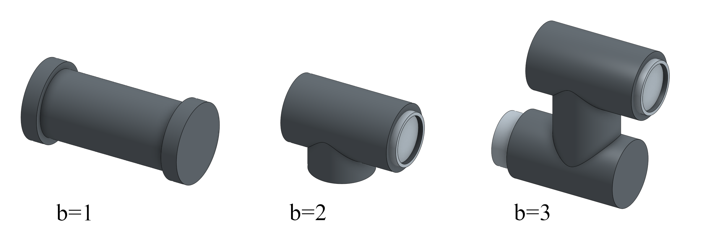
Figure 2: Exemplary modules with $b\in\{1,2,3\}$ bodies.

Throughout this work, we aim to find a composition of heterogeneous modules that can be assembled into a robot to solve a given task. We assume that a module $m$ has $b$ bodies connected by $b-1$ joints and a proximal and distal connector $\{c_{p},c_{d}\}$, defining interfaces to connect it to other modules. Our method explicitly permits the inclusion of empty bodies, enabling the creation of more complex module structures. For instance, this flexibility allows the combination of two linear joints with an empty body to construct a planar joint, which can be used to model a mobile base module. Examples of modules with $b\in\{1,2,3\}$ are shown in Fig. 2. We consider two special types of modules, bases and end effectors: For base modules, $c_{p}$ represents the reference frame of the base; for end effector modules, $c_{d}$ defines the tool center point (TCP). Any connector is attached to a body and has a fixed type. The corresponding modules can be connected if a distal and a proximal connector have the same type. In this work, we consider any MR that adheres to the following structure:

Base - $M$ - … - $M$ - End Effector

Here, $M$ are arbitrary regular modules, so the structure fits any serial manipulator with exactly one base and end effector module. An assembled composition of $n_{M}$ modules is referred to as robot $R=(m_{1},\dots,m_{n_{M}})$.

A task $T$, as displayed in Fig. 3, is defined by the tuple $\langle G,\mathcal{T},\mathcal{O}\rangle$, where $G=(g_{1},\dots,g_{n_{G}})$ is a sequence of goals, $\mathcal{T}$ is a set of tolerances for all goals, and $\mathcal{O}$ is the workspace occupied by obstacles. Joint limits for a robot with $n_{J}$ joints are given by lower limits $\underline{\boldsymbol{q}}\in\mathbb{R}^{n_{J}}$ and upper limits $\overline{\boldsymbol{q}}\in\mathbb{R}^{n_{J}}$. We define the set of all valid joint configurations as $\mathcal{Q}=\left[\underline{\boldsymbol{q}},\overline{\boldsymbol{q}}\right]$. A goal $g\in G\subset SE3$ is defined as a position $\boldsymbol{p}_{g}\in\mathbb{R}^{3}$ and a desired orientation $\boldsymbol{n}_{g}\in SO3$. We introduce the operator

$$rot(\boldsymbol{n_{1}},\boldsymbol{n_{2}})=\langle\boldsymbol{e},\theta\rangle,\|\boldsymbol{e}\|_{2}=1,\theta\in[0,\pi]$$ (1)

that returns the rotation from $\boldsymbol{n_{1}}$ to $\boldsymbol{n_{2}}$ in axis-angle representation, defined as a unit vector $\boldsymbol{e}$ and an angle $\theta$. The tolerances $\mathcal{T}$ are composed of a position tolerance $t_{p}\in\mathbb{R}_{+}$ and an orientation tolerance, given as $t_{o}=\langle\boldsymbol{t},\varphi\rangle,\boldsymbol{t}\in\{\boldsymbol{x}\in\mathbb{R}_{+}^{3}\mid\|\boldsymbol{x}\|_{\infty}\leq 1\},\varphi\in(0,\pi]$. Further, we define the forward kinematics (FK) for robot $R$ with joint angles $\boldsymbol{q}$ as

$$[\boldsymbol{p}_{\text{TCP}},\boldsymbol{n}_{\text{TCP}}] =FK(R,\boldsymbol{q})\,,$$ (2)

with TCP position $\boldsymbol{p}_{\text{TCP}}\in\mathbb{R}^{3}$ and TCP orientation $\boldsymbol{n}_{\text{TCP}}\in SO3$. We denote the workspace occupied by the robot as $\mathcal{A}(R,\boldsymbol{q})$.

A goal $g$ can be be reached by robot $R$, if there exists a joint configuration $\boldsymbol{q}\in\mathcal{Q}$ such that

$$\|p_{\text{TCP}}(R,\boldsymbol{q})-\boldsymbol{p}_{g}\|_{2}\leq t_{p}\land\theta~{}|\boldsymbol{e}|\leq\varphi~{}\boldsymbol{t}\,,$$ (3)

where $\langle\boldsymbol{e},\theta\rangle=rot(\boldsymbol{n}_{g},\boldsymbol{n}_{\text{TCP}})$. In (3), $|\boldsymbol{e}|$ denotes the element-wise absolute value and the inequality holds if it is true for all dimensions. We denote this property as $r(R,\boldsymbol{q},g,\mathcal{T})$ which returns true, if robot $R$ reaches goal $g$ with the joint configuration $\boldsymbol{q}$ and false, otherwise. We also introduce the condition $\hat{r}$ that determines whether a trajectory $\boldsymbol{q}(t)$ reaches all goals in the order specified by $G$ as

$$\hat{r}(R,\boldsymbol{q}(t),G,\mathcal{T})=\exists\left(t_{1},\dots,t_{n}\right)\mid$$ (4)

$$\qquad t_{1}\leq t_{2}\leq\dots\leq t_{n}=t_{max}$$

$$\quad\land\forall i\in\{1,\dots,n\}:r(R,\boldsymbol{q}(t_{i}),g_{i},\mathcal{T})\,.$$

A task $T$ is considered to be achieved by robot $R$, if there exists a trajectory $\boldsymbol{q}(t)$ that is collision-free (5a), for which joint velocity (5b), acceleration (5c), and torque limits (5d) are met, and for which all goals are reached in the intended order (5e). We denote the set of all trajectories fulfilling these properties by:

$$\chi_{T}(R)=\{ \boldsymbol{q}(t):[0,t_{max}]\to\mathcal{Q}\mid$$ (5)

$$\mathcal{O}\cap\mathcal{A}(R,\boldsymbol{q}(t))=\emptyset$$ (5a)

$$\land\dot{\boldsymbol{q}}(t)\in\left[\,\dot{\underline{\boldsymbol{q}}},\dot{\overline{\boldsymbol{q}}}\,\right]$$ (5b)

$$\land\ddot{\boldsymbol{q}}(t)\in\left[\,\ddot{\underline{\boldsymbol{q}}},\ddot{\overline{\boldsymbol{q}}}\,\right]$$ (5c)

$$\land|\boldsymbol{\tau}|\leq\boldsymbol{\tau}_{max}$$ (5d)

$$\land\hat{r}(R,\boldsymbol{q}(t),G,\mathcal{T}\}\,.$$ (5e)

If $\chi_{T}(R)\neq\emptyset$, we assume there is a path planning algorithm $p_{T}(R)=\boldsymbol{q}(t)$ that computes a trajectory $\boldsymbol{q}(t)$ for task $T$ with the robot $R$. Under this assumption, we can define our objective function

$$C_{T}(R)=w_{s}C_{s}(R)+w_{p}C_{p,T}(R,p_{T}(R))\,,$$ (6)

which is composed of a weighted sum of robot setup costs $C_{s}$ (such as acquisition cost or module availability) and process cost $C_{p,T}$ (such as cycle time or energy consumption) arising during operation. Consequently, the robot defined by the optimal composition is given by

$$R_{T}^{*} =\operatorname*{arg\,min}_{R}(C_{T}(R)),~{}p_{T}(R)\in\chi_{T}\,.$$ (7)

III Method

In a GA, multiple solution candidates (chromosomes) form the population, which is altered via the genetic operators in every generation. To encode a manipulator as chromosome $c$ of fixed length $n_{c}$, we index the set of available modules $\mathcal{M}$ and write $c=(m_{1},\dots,m_{n_{c}}),m_{i}\in\{0,1,\dots,|\mathcal{M}|\}$, where $m_{i}=j,j\in\{1,\dots,|\mathcal{M}|\}$ encodes module $M_{j}\in\mathcal{M}$. In a slight abuse of notation, we will use a gene $m_{i}$ and the encoded module $M_{i}$ interchangeably in the remainder of this paper. Notably, a gene encodes an empty slot when set to zero ($m_{i}=0$). That is, a series of genes $(u,0,v)$ encodes a partial configuration of modules $(M_{u},M_{v})$. This flexibility is crucial, as it allows us to encode any manipulator with $n_{M}$ modules in a chromosome of length $n_{c}\geq n_{M}$. As a result, we neither predetermine the number of modules in a solution candidate nor constrain the search space to alternate joint and link modules, allowing us to explore unconventional compositions.

III-A Genetic Operators

Within every generation, we compute the fitness value for every chromosome. Based on the fitness, we perform steady state selection: The $p$ solution candidates (population) with the highest fitness among all individuals are chosen to be the parents for the next generation. We then replace any chromosome not selected by a new one created by a single-point crossover between two randomly selected parents. We denote the set of all modules with the same connectors as a module $m$ by $\mathcal{V}_{m}$ and, finally, select a replacement candidate uniformly from $\mathcal{V}_{m}$ for every gene in the current population with a mutation probability of $p_{m}$. If the mutated chromosome $m_{i}$ is neither a base nor an end effector ($i\notin\{1,n_{c}\}$), the empty slot module is added to $\mathcal{V}_{m}$ if a connection between the adjacent modules $(m_{i-1},m_{i+1})$ is possible. Due to the inherent validity check of connections during population generation, we can incorporate constraints on module composition, such as those given by connector properties inherently, and before computing the fitness. Therefore, even complex module libraries, e.g., modules of different sizes, can be optimized using our GA.

III-B Fitness Function

As the fitness function $f$ determines the quality of a solution candidate, we expect the relation $C_{T}(R_{i})<C_{T}(R_{j})\Leftrightarrow f(R_{i})>f(R_{j})$ between fitness and task cost to hold. However, due to the computationally expensive evaluation of the cost function in (6) that requires attempting to compute a solution trajectory, it is infeasible to use it directly as a fitness function. Given that our selection process relies on the order of fitness scores rather than their exact numerical values, we implement a lexicographic fitness function [30]: We select a sequence of fitness objectives $f(R)=\langle f_{1}(R),\dots,f_{n}(R)\rangle$, ranked descending by importance and computational simplicity, and define the ordering

$$f(R_{a})>f(R_{b})\Leftrightarrow \exists k\in\{1,\dots,n\}:f_{k}(R_{a})>f_{k}(R_{b})$$

$$\land\forall i<k:f_{i}(R_{a})=f_{i}(R_{b})\,,$$ (8)

$$f(R_{a})=f(R_{b})\Leftrightarrow \forall i\in\{1,\dots,n\}:f_{i}(R_{a})=f_{i}(R_{b})\,.$$ (9)

As an illustrative example, let us consider two robots, $R_{1}$ and $R_{2}$, and evaluate them on two objectives. The first objective, $f_{1}(R)$, is a binary classifier determining whether a trajectory $\boldsymbol{q}(t)\in\chi_{T}(R)$ exists for each robot. The second objective, $f_{2}(R)=-n_{J}(R)$, is defined as the negative of the number of joints for each robot. Applying a lexicographic ordering, $R_{1}$ is preferred over $R_{2}$ if a trajectory exists for $R_{1}$ but not for $R_{2}$ or if a trajectory exists for both robots, but $R_{1}$ has fewer joints than $R_{2}$.

Specifically, we introduce the following objectives for a robot $R$:

• Trivial reachability: A goal can only be reached if a robot arm is sufficiently long. We introduce the maximum Euclidean distance between the distal and the proximal connector of module $M_{i}$ as $d_{max}(M_{i})$ and define

  $$f_{1}(R)=\begin{cases}1\text{, if }\sum_{R}d_{max}(M_{i})\geq\max_{g\in G}{\|\boldsymbol{p}_{g}\|_{2}}\\ 0\text{, otherwise.}\end{cases}$$ (10)

• Reachable number of goals: Objective

  $$f_{2}(R)=\sum_{g\in G}\left(\begin{cases}1\text{, if }\exists\boldsymbol{q}\in\mathcal{Q}:r(R,\boldsymbol{q},g,\mathcal{T})\\ 0\text{, otherwise}\end{cases}\right)$$ (11)

  returns the number of goal positions that can be reached by the robot $R$. The existence of a valid joint configuration $\boldsymbol{q}$ is determined using a numeric inverse kinematics algorithm.

• Reachable number of goals, considering collisions: Objective

  $$f_{3}(R)=\sum_{g\in G}\left(\begin{cases}1\text{, if }\exists\boldsymbol{q}\in\mathcal{Q}:&r(R,\boldsymbol{q},g,\mathcal{T})\\ &\land\mathcal{O}\cap\mathcal{A}(R,\boldsymbol{q})=\emptyset\\ 0\text{, otherwise}\end{cases}\right)$$ (12)

  returns the number of goal positions that can be reached while there are no collisions between robot and environment.

• Cost objective: The final fitness objective measures robot setup complexity and task performance and can be chosen freely. Following (6), (7), we define

  $$f_{4}(R)=\begin{cases}-\infty,&\text{if }\chi_{T}(R)=\emptyset\\ -C_{T}(R),&\text{otherwise.}\end{cases}$$ (13)

These criteria allow us to determine its fitness hierarchically and stop evaluation if it does not achieve the maximum fitness value $f_{i}(R)\neq f_{i,max}$ for an intermediate objective $i\leq 3$, where $f_{1,max}=1$, $f_{2,max}=f_{3,max}=|G|$. However, unlike prior work using hierarchical elimination for the optimization of MR compositions [7], we retain information about partial solutions, such as the ability to reach the final goal in the task and use it for the selection process. Moreover, the introduction of a lexicographic fitness function enhances interpretability. Rather than managing and fine-tuning weighted sums for numerous task criteria for a scalar fitness value, a human evaluator can easily conclude which constraints different solution candidates satisfy.

IV Experiments

IV-A Robot Modules

For our experiments, we use data from 29 different modules manufactured by RobCo. The set consists of four different bases, 20 different static link modules, four modules with a joint, and one end effector. The static link modules differ in size and shape (L-shaped and I-shaped), and the bases differ in size and mounting orientation. The database can be divided into six large modules, including two bases, and 22 smaller modules, including the end effector that can only be attached to one of the large modules using a special connecting link module. Without the constraints imposed by the connectors and the necessity of a base and end effector module, there would be $\sum_{i=n}^{12}29^{n}\approx 10^{17}$ distinct compositions with at most twelve modules that can be built from this module set. Considering the different module sizes and types, the resulting size of the workspace is still beyond $10^{12}$ (one trillion) possible compositions for a chromosome length of twelve and, to the best of our knowledge, exceeds those in prior work, such as 15552 in [7], 32768 in [5], and around $10^{6}$ in [6] significantly.

IV-B Task Definition

(a) Synthetic I, $d=4$

(b) Synthetic II, $d=3$

(c) Manufacturing I

(d) Manufacturing II

Figure 3: We evaluate our algorithm on two synthetic and two manufacturing settings: Synthetic obstacles are shown in red, milling machines and conveyor belts are shown in grey. Every goal consists of a desired position and orientation, indicated by an end effector. The robot base placement is indicated by a red base module.

We evaluate our approach on two types of tasks: Randomly generated synthetic tasks and manually curated industrial manufacturing tasks. We evaluate the algorithm’s performance for each type in two different settings and three difficulty levels each. Fig. 3 shows an example for every type of task.

For the first setting (Synthetic I), we implement a scenario similar to the one proposed in [6] by discretizing a space of $1.25\text{m}^{3}$, centered in the point $[0,0,0.625]^{T}\text{m}$ in $5\times 5\times 5$ voxels of edge width $0.25\text{m}$. For the different difficulty levels, we randomly sample $d\in\{3,4,5\}$ box-shaped obstacles, filling one voxel each and $d$ goal positions centered in a voxel each. In addition, we create non-discretized synthetic tasks (Synthetic II), where goal and obstacle position and orientation are sampled randomly in a half-ball of radius $1.2m$ and with a positive $\mathrm{z}$ coordinate. In this setting, obstacles can be spheres, boxes, or cylinders, and their position and volume are determined randomly. For all goals in the synthetic tasks, we set the orientation tolerance to half a degree around an arbitrary axis ($\boldsymbol{e}=[1,1,1]^{T},\varphi=\frac{\pi}{360}$). Finally, we apply a simple, non-exhaustive heuristic to discard tasks that are not solvable, e.g., because obstacles cover one of the goal positions or the base position. In total, we define 120 synthetic tasks, 20 for each setting with $d\in\{3,4,5\}$.

Furthermore, we evaluate our approach in two settings inspired by real-world machine tending problems (Manufacturing I & II), where the goals represent a pick position for raw material, a position inside a milling machine, and a position to place the final workpiece on. For each one, the difficulty level is determined by using one of three orientation tolerances, mimicking different workpiece geometries:

• Sphere-like geometry $(t_{o}=t_{o,1})$: The TCP orientation can be chosen freely within an arbitrary rotation of 90°, setting $\boldsymbol{e}_{1}=[1,1,1]^{T},\varphi_{1}=\frac{\pi}{2}$.

• Partially symmetric geometry $(t_{o}=t_{o,2})$: The TCP orientation is free around its $\mathrm{z}$-axis but otherwise constrained, setting $\boldsymbol{e}_{2}=[\frac{1}{360},\frac{1}{360},1]^{T},\varphi_{2}=\pi$.

• Arbitrary geometry $(t_{o}=t_{o,3})$: The TCP orientation is pre-determined and we allow a minor deviation only, setting $\boldsymbol{e}_{3}=[1,1,1]^{T},\varphi_{3}=\frac{\pi}{360}$.

For all tasks in this paper, we set a position tolerance of $t_{p}=10^{-3}\text{m}$.

IV-C Baseline

We compare our approach to a two-level GA based on hierarchical elimination, as proposed in [7]. We eliminate unfit solution candidates that cannot reach the first and last goal as indicated by (12) before evaluation. Instead of utilizing the previously introduced lexicographic fitness function, we adopt [7, (3)-(10)]. Consequently, the baseline fitness function depends on weighting factors $k_{i}$, linear distance $L$, angular distance $A$, dexterity $D$, robot mass $M$, joint value differences $V$, and the percentage of reachable intermediate points $P$:

$$f_{B}=e^{-\left(k_{1}R+k_{2}L+k_{3}A+k_{4}D+k_{5}M+k_{6}V\right)}+k_{7}P\,.$$ (14)

We waive the obstacle proximity criterion initially introduced in the referenced work, which is defined solely for spherical obstacles, and replace the involved module criterion $I$ by the robot mass $M$ to accommodate heterogeneous module geometries. All other criteria remain as defined in the reference. In the second optimization step, we select the best 25 individuals for each scenario and compute trajectories using the same method as employed for our solutions.

IV-D Setup

All experiments are conducted using Timor-Python [29] on a desktop PC with an Intel i7-11700KF processor. For trajectory generation, we follow the method from [31] in combination with the RRT-Connect planner provided by the Open Motion Planning Library (OMPL) [32] with a timeout of 3 seconds.

For all tasks, we define the optimization criterion as a function of the number of robot joints $n_{J}$, robot modules $n_{M}$, and trajectory cycle time $t_{max}$ as:

$$C_{T}=n_{J}+0.2n_{M}+t_{max}\,.$$ (15)

Thereby, we optimize for setup and process cost and assume that $1.2s$ of cycle time is approximately equally valuable as creating a manipulator with one joint less. The algorithm runs for 200 generations on a population size of 25, which is initialized using weighted random sampling, where each initial module has a probability of $p_{j}=0.9$ to contain a joint. For evaluating the performance on the manufacturing tasks, we perform optimization over ten random seeds, whereas due to run time constraints, we run optimization once on all synthetic tasks. If not stated otherwise, all results refer to the mean computed over the difficulty levels $d\in\{3,4,5\}$ for synthetic tasks and for tolerances $t_{o,1}$, $t_{o,2}$, and $t_{o,3}$ for the manufacturing tasks with differing seeds.

IV-E Results

TABLE I: Our approach outperforms the baseline in terms of achieved tasks, average cycle time, and average number of joints for the resulting robot compositions.

		Achieved	$C_{T}$	$n_{J}$	$t_{max}$
Synthetic I	$d=3$	16	11.86	6.2	3.1s
	$d=4$	10	15.16	6.8	5.7s
	$d=5$	10	16.42	6.7	7.1s
Synthetic II	$d=3$	20	12.27	6.4	3.3s
	$d=4$	20	13.80	6.7	4.6s
	$d=5$	20	15.33	6.8	5.9s
Ours (average over all)		16	14.14	6.6	5.0s
Baseline		15.2	19.67	8.1	15.2s
Manufacturing I	$t_{o,1}$	10	12.81	5.3	5.0s
	$t_{o,2}$	10	14.33	6.7	5.0s
	$t_{o,3}$	10	15.05	6.6	5.8s
Manufacturing II	$t_{o,1}$	10	10.15	4.5	3.4s
	$t_{o,2}$	10	12.48	6.4	3.6s
	$t_{o,3}$	10	12.27	6.0	3.8s
Ours (average over all)		10	12.85	5.9	4.5s
Baseline		9.8	20.06	7.5	15.0s
$C_{T}$: Cost as defined in eq. (15), $n_{J}$: Number of joints, $t_{max}$: Cycle time

The evaluation took $960ms$ per individual on average, resulting in 1.2 hours for one optimization over 200 generations. This provides a significant speedup compared to determining the cost function for every individual and running into the path planner’s 3s time limit for every unfit solution candidate. Table I reports the number of achieved tasks over the different settings and the average lowest cost for all tasks with a valid solution. In addition, we report the mean number of joints $n_{J}$ and cycle time $t_{max}$ for all solutions with minimal cost. We aggregate all synthetic and manufacturing task runs and compare them to the baseline according to section IV-C.

Our algorithm finds a valid solution for 80% of the synthetic tasks. Upon manual inspection, we discover that some of the remaining tasks are inherently unsolvable due to the proximity of goals and obstacles. For the hand-curated industrial tasks, our optimization resulted in valid solutions for every trial.

On average, our algorithm yields solutions with costs about 30% lower than those generated by our baseline method. These cost reductions result from simplified robot designs and substantial decreases in cycle times. Specifically, for the synthetic tasks, our approach reduces the average number of joints by 1.5 and decreases cycle times by 67%. In manufacturing tasks, we observe an average reduction of 1.6 joints and a decrease in cycle times by 70%. This result strongly indicates that including trajectory cycle time in the optimization process, as described in (13), provides a significant advantage over the two-level approach deployed for the baseline.

Notably, the robots’ complexity changes with the task difficulty. Two different robots for the “Manufacturing II” setting with $t_{o}=t_{o,1}$ and $t_{o}=t_{o,3}$ are shown in Fig. 1. Regardless of the orientation tolerances, the selection of a vertically mounted base followed by at least one static link resulted in trajectories with minimal cycle time. Neither of the solutions shown would have been possible if structural constraints, as used in [6, 7, 5], had been enforced.

V Conclusion

This paper presents a genetic algorithm with a lexicographic fitness function for the task-based optimization of modular manipulators. Compared to existing approaches, we impose no prior assumptions on the structure or the number of modules in an optimal solution. By designing a computationally efficient fitness evaluation, our approach can handle complex scenarios and search spaces exceeding those presented in the related literature by magnitudes. Our experimental validation shows that our GA can find solutions adapted to the complexity of a task. Moreover, the unconventional but high-performant module compositions resulting from optimizing MR for manufacturing tasks with broad orientation tolerances showcase that use-case-tailored MRs do not necessarily follow human intuition. Our approach applies to all kinds of serially connected MRs, regardless of module complexity. Additional task constraints can easily be integrated by extending the intermediate objectives evaluated during fitness computation. Lastly, our method can be used for any task without the necessity of simplification, e.g., via discretization.

References

- [1] M. R. Pedersen, L. Nalpantidis, R. S. Andersen, C. Schou, S. Bøgh, V. Krüger, and O. Madsen, “Robot skills for manufacturing: From concept to industrial deployment,” Robotics and Computer-Integrated Manufacturing, vol. 37, pp. 282–291, 2015.
- [2] D. Gorecky, S. Weyer, A. Hennecke, and D. Zühlke, “Design and instantiation of a modular system architecture for smart factories,” IFAC-PapersOnLine, vol. 49, no. 31, pp. 79–84, 2016.
- [3] L. Ribeiro and M. Bjorkman, “Transitioning from standard automation solutions to cyber-physical production systems: An assessment of critical conceptual and technical challenges,” IEEE Systems Journal, vol. 12, no. 4, pp. 3816–3827, 2018.
- [4] M. Yim, W.-M. Shen, B. Salemi, D. Rus, M. Moll, H. Lipson, E. Klavins, and G. S. Chirikjian, “Modular self-reconfigurable robot systems [grand challenges of robotics],” IEEE Robotics and Automation Magazine, vol. 14, no. 1, pp. 43–52, 2007.
- [5] M. Althoff, A. Giusti, S. B. Liu, and A. Pereira, “Effortless creation of safe robots from modules through self-programming and self-verification,” Science Robotics, vol. 4, no. 31, 2019.
- [6] J. Whitman, R. Bhirangi, M. Travers, and H. Choset, “Modular robot design synthesis with deep reinforcement learning,” in Proc. of the AAAI Conf. on Artificial Intelligence (AAAI), vol. 34, no. 06, 2020, pp. 10 418–10 425.
- [7] E. Icer, H. Hassan, K. El-Ayat, and M. Althoff, “Evolutionary cost-optimal composition synthesis of modular robots considering a given task,” in Proc. of the IEEE/RSJ Int. Conf. on Intelligent Robots and Systems (IROS), 2017, pp. 3562–3568.
- [8] M. Mayer, J. Külz, and M. Althoff, “CoBRA: A composable benchmark for robotics applications,” arXiv:2203.09337 [cs.RO], 2022.
- [9] G. Pritschow and K. Tuffentsammer, “A new modular robot system,” CIRP Annals, vol. 35, no. 1, pp. 89–92, 1986.
- [10] T. Fukuda, S. Nakagawa, Y. Kawauchi, and M. Buss, “Self organizing robots based on cell structures – CEBOT,” in Proc. of the Int. Workshop on Intelligent Robots (IROS), 1988, pp. 145–150.
- [11] D. Schmitz, P. Khosla, and T. Kanade, “The CMU reconfigurable modular manipulator system,” Tech. Rep. 88–7, 1988.
- [12] C. Nainer, M. Feder, and A. Giusti, “Automatic generation of kinematics and dynamics model descriptions for modular reconfigurable robot manipulators,” in IEEE Int. Conf. on Automation Science and Engineering (CASE), vol. 17, 2021, pp. 45–52.
- [13] T. Zhang, Q. Du, G. Yang, C. Wang, C.-Y. Chen, C. Zhang, S. Chen, and Z. Fang, “Assembly configuration representation and kinematic modeling for modular reconfigurable robots based on graph theory,” Symmetry, vol. 14, no. 3, 2022.
- [14] A. Yun, D. Moon, J. Ha, S. Kang, and W. Lee, “ModMan: An advanced reconfigurable manipulator system with genderless connector and automatic kinematic modeling algorithm,” IEEE Robotics and Automation Letters, vol. 5, no. 3, pp. 4225–4232, 2020.
- [15] E. Romiti, J. Malzahn, N. Kashiri, F. Iacobelli, M. Ruzzon, A. Laurenzi, E. M. Hoffman, L. Muratore, A. Margan, L. Baccelliere, S. Cordasco, and N. Tsagarakis, “Toward a plug-and-work reconfigurable cobot,” Transactions on Mechatronics, vol. 27, no. 5, pp. 2319–3231, 2022.
- [16] A. Dogra, S. Padhee, and E. Singla, “Optimal synthesis of unconventional links for modular reconfigurable manipulators,” Journal of Mechanical Design, vol. 144, no. 8, 2022.
- [17] S. B. Liu and M. Althoff, “Optimizing performance in automation through modular robots,” in Proc. of the IEEE Int. Conf. on Robotics and Automation (ICRA), 2020, pp. 4044–4050.
- [18] C. J. J. Paredis and P. K. Khosla, “Synthesis methodology for task based reconfiguration of modular manipulator systems,” in Proc. of the Int. Symp. on Robotics Research (ISRR), 1993.
- [19] A. Valente, “Reconfigurable industrial robots: A stochastic programming approach for designing and assembling robotic arms,” Robotics and Computer-Integrated Manufacturing, vol. 41, pp. 115–126, 2016.
- [20] S. Singh, A. Singla, and E. Singla, “Modular manipulators for cluttered environments: A task-based configuration design approach,” Journal of Mechanisms and Robotics, vol. 10, no. 5, 2018.
- [21] E. Icer and M. Althoff, “Cost-optimal composition synthesis for modular robots,” in Proc. of the IEEE Conference on Control Applications (CCA), 2016, pp. 1408–1413.
- [22] E. Icer, A. Giusti, and M. Althoff, “A task-driven algorithm for configuration synthesis of modular robots,” in Proc. of the IEEE Int. Conf. on Robotics and Automation (ICRA), 2016, pp. 5203–5209.
- [23] D. E. Goldberg and J. H. Holland, “Genetic algorithms and machine learning,” Machine Learning, vol. 3, pp. 95–99, 1988.
- [24] K. Sims, “Evolving virtual creatures,” in Proc. of the Ann. Conf. on Computer Graphics and Interactive Techniques (SIGGRAPH), vol. 21, 1994, pp. 15–22.
- [25] H. Lipson and J. B. Pollack, “Automatic design and manufacture of robotic lifeforms,” Nature, vol. 406, pp. 974–978, 2000.
- [26] J. Han, W. K. Chung, Y. Youm, and S. H. Kim, “Task based design of modular robot manipulator using efficient genetic algorithm,” in Proc. of the IEEE Int. Conf. on Robotics and Automation (ICRA), 1997, pp. 507–512.
- [27] O. Chocron and P. Bidaud, “Evolutionary algorithms in kinematic design of robotic systems,” in Proc. of the IEEE/RSJ Int. Conf. on Intelligent Robots and Systems (IROS), vol. 2, 1997, pp. 1111–1117.
- [28] O. Chocron, “Evolutionary design of modular robotic arms,” Robotica, vol. 26, no. 3, pp. 323–330, 2008.
- [29] J. Külz, M. Mayer, and M. Althoff, “Timor Python: A toolbox for industrial modular robotics,” in Proc. of the IEEE/RSJ Int. Conf. on Intelligent Robots and Systems (IROS), 2023, in press.
- [30] C. A. Coello, “An updated survey of GA-based multiobjective optimization techniques,” ACM Computing Surveys, vol. 32, no. 2, pp. 109–143, 2000.
- [31] T. Kunz and M. Stilman, “Time-optimal trajectory generation for path following with bounded acceleration and velocity,” in Robotics: Science and Systems, 2012.
- [32] I. A. Şucan, M. Moll, and L. E. Kavraki, “The open motion planning library,” IEEE Robotics and Automation Magazine, vol. 19, no. 4, pp. 72–82, 2012.