Fractional Advection Diffusion Asymmetry Equation, derivation, solution and application
Abstract
The non-Markovian continuous-time random walk model, featuring fat-tailed waiting times and narrow distributed displacements with a non-zero mean, is a well studied model for anomalous diffusion. Using an analytical approach, we recently demonstrated how a fractional space advection diffusion asymmetry equation, usually associated with Markovian Lévy flights, describes the spreading of a packet of particles. Since we use Gaussian statistics for jump lengths though fat-tailed distribution of waiting times, the appearance of fractional space derivatives in the kinetic equation demands explanations provided in this manuscript. As applications we analyse the spreading of tracers in two dimensions, breakthrough curves investigated in the field of contamination spreading in hydrology and first passage time statistics. We present a subordination scheme valid for the case when the mean waiting time is finite and the variance diverges, which is related to Lévy statistics for the number of renewals in the process.
1 Introduction
Continuous-time random walk [1, 2, 3, 4, 5, 6, 7, 8, 9, 10, 11] (CTRW) is a stochastic jump process for a random walk that jumps instantaneously from one site to another, following a sojourn period on a site. See also recent works in [12, 13, 14, 15, 16, 17, 18, 19, 20, 21]. For example, it was used to describe dispersive transport in time of flight experiment of charge carriers in disordered systems [22]. The non-Markovian characteristic of CTRW becomes apparent, especially when the disorder is introduced into the system, as observed in the sense of ensemble average [10]. Fractional kinetic equations [23, 4, 24, 25, 26, 27, 28, 29] are a popular tool used to describe various anomalous phenomena [30, 31]. When the bias of the system is a constant, the fractional time diffusion equation follows [32, 33]
| (1) |
describing anomalous dynamics with . Here we make the assumption that both the generalized mobility and the generalized diffusion coefficient are set to one. The time Riemann-Liouville operator introduces a convolution integral involving a power-law kernel that decays slowly over time, which is related to memory effects of this nonequilibrium system. In addition, is directly governed by heavy-tailed power law waiting times distributions
| (2) |
in the context of the underlying picture, the CTRW model.
Due to heavy-tailed waiting times, characterized by an infinite mean, Eq. (1) illustrates sub-diffusion behaviors. However, our focus is on the super-diffusion scenario. Our recent findings demonstrated that the positional distribution, , of the mentioned CTRW model follows the fractional advection diffusion asymmetry equation (FADAE)
| (3) |
for .
Here , , and are transport coefficients to be discussed, and the operator is the right Riemann-Liouville derivative [34, 35] in regard to space. Thus the fat tailed distribution of sojourn times Eq. (2), which leads to the fractional time Fokker-Planck equation (1), when , can lead as shown here to the fractional space differential equation (3) if . There is a transition in the basic kinetic description of the transport. When the mean waiting time diverges, we get the mentioned fractional time Fokker-Planck equation. However, if the mean sojourn time is finite but the variance diverges, we obtain a fractional space description. Our first goal is to clarify this point.
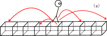
Fractional space transport equations [34, 36, 37, 4, 38, 30, 39, 40] are usually associated with Lévy flights [35, 41, 42, 43, 44, 45, 46, 47, 48]. See subplot (a) in Fig. 1. The term Lévy flights, also referred to as Lévy motion, was coined by Benoit Mandelbrot in honour of the French mathematician Paul Lévy. The individual jump has a length that is distributed with the PDF decaying at large positions as a fat-tailed jump length distribution with diverging variance of the size of the jumps. Importantly, the Lévy flight process is a Markovian process, hence the appearance of the fractional framework in the context of a model with fat tailed distributions of waiting times is of interest. In particular, any fitting of data using the fractional space kinetic equation, cannot be used as strong evidence for Lévy flights, or for a basic Markovian underlying process.
Subordination methods, based on an integral transformation, present a way of solving fractional kinetic equations [3, 49, 50, 51, 52, 53, 54, 55, 56, 57]. To be more exact, when the mean waiting time diverges [33], subordination methods map a classical Fokker-Planck equation onto a fractional diffusion one with the fractional time derivative. For this case, the term ”inverse Lévy transform” is sometimes used due to the number of renewals that follows the inverse one-sided Lévy distribution. This well-known framework works when . We will propose a new subordination method to solve a wide range of problems valid when the mean waiting time is finite, but the variance is diverging, namely the case .
The paper is organized as follows. We start by introducing the CTRW model and give the corresponding concepts in Sec. 2. We derive the corresponding FADAE and give our explanations in Sec. 3. In Sec. 4, the applications and extensions of Eq. (3) are considered, ranging from the FADAE in two dimensions, the positional distribution with the time-dependent bias and variance, breakthrough curves, and the first passage time obtained from subordination methods. Three limiting laws of FADAE, describing the large asymmetric parameter , the large diffusion term , and the general typical fluctuations, are discussed in Sec. 5. To conclude, we summarize our findings in Sec. 6.
2 CTRW model
Now we define the CTRW model [4, 58, 10] discussed in this manuscript. Let us consider the process starting at with the initial position . A walker is trapped on the origin for time , then makes a jump and the displacement is ; the walker is further trapped on for time , and then jumps to a new position; this process is then repeated. Thus, the process is characterized by a set of waiting times and the displacements , where is the backward recurrence time [59, 60] and the time dependent is the number of renewals from the observation time zero to . Specifically, . These random variables, i.e., and are mutually independent and identically distributed (IID) random variables with common PDFs and , respectively. Consider the broad distribution characterized by a fat tail
| (4) |
where is a time scale and the power-law index . This indicates that the mean is finite, but not the variance. The Laplace transform will be used in solving our problems. It is defined by for a well behaved function . The Laplace transform of , , is [4, 59]
| (5) |
with . For , we can check that , which indicates that in Eq. (4) is normalized.
For the displacement PDF , we assume has a finite mean and the variance . In this manuscript, we consider a Gaussian distribution
| (6) |
In Fourier space, with . Thus, the small expansion of reads
| (7) |
When the sojourn time PDF has a fat tail and the variance of the displacement is finite, a wide range of anomalous behaviors emerge [3, 61]. As mentioned, here we will focus on the widely applicable case [62, 63, 64, 65, 66, 67, 68, 69].
3 Fractional-Space Advection Diffusion Asymmetry Equation
3.1 Calculation of the Positional distribution
We now consider the CTRW model and note that the PDF of the position of a walker at time is
| (8) |
where denotes the probability of the number of events during the time interval and is the probability that the walker is on conditioned that it made steps. Equation 8 is known as the subordination of the spatial process by the temporal process for [3, 33, 70, 54]. The technique was used in computer simulation in the context of fractional Fokker-Planck dynamics [71], random diffusivity [56], population heterogeneity [72] and one-dimensional Brownian search problem [55]. As mentioned before, time intervals and displacements of walkers under investigation are IID with common PDFs and , respectively. Note the relation between and , i.e., , and the density of the particle’s displacement after the first step is given exactly by , i.e., . Then using the convolution of the Fourier transform, it follows that as well known
| (9) |
Based on the renewal process [59], in Laplace space follows . Considering the random variable and taking the inverse transform, then typical fluctuations follow [73, 59, 60]
| (10) |
with
| (11) |
Eq. (10) is valid in the limit of . Rare fluctuations describing the scaling of were investigated in Ref. [60]. Here is the Lévy distribution [34, 35], defined by
| (12) |
Utilizing Eqs. (8), (9) and (10), we have
| (13) |
Note that Eq. (13) can be extended to more general situations, e.g. if the jump size distribution is fat-tailed. Starting from Eq. (13) and changing variable , we get
| (14) |
describing the scaling when . Note that in the long time limit, the lower limit of the integral in Eq. (14) can be replaced with ; see Eq. (21) below. The reason is as follows the dimensionless parameter
| (15) |
for when . The scaling form of the position reads
| (16) |
with
| (17) |
and
| (18) |
In the long time limit, Eq. (16) reduces to the well-known result [73, 74]
| (19) |
where we used the fact that tends to when from Eq. (19). More precisely, Eq. (19) is valid for the fixed , , and the long observation time . At the same time, we will consider a second dimensionless parameter ,
| (20) |
which quantifies the convergence to the Lévy distribution. We will then discuss three limits. If , Eq. (16) gives Eq. (19). However, assume a situation when the bias is weak meaning is very large, this is important in many applications that we consider, and corresponds to the linear response regime when the external driving force determined by is small. Then the last limit will be to consider a long time but finite. In this case, Eq. (14) is valid. Refer to Appendix A for more detailed discussions on .
3.2 Derivation of Fractional-Space Advection Diffusion asymmetry Equation
Rewriting Eq. (14) with a lower limit , in the long time limit we get
| (21) |
see Fig. 2. Here we use the expression to denote the positional distribution in the long time limit. The statistic of at a short time is now discussed. For this case, Eq. (21) reduces to
| (22) |
where we ignored the terms and in Eq. (21).
It implies that for small the Gaussian distribution is found. Besides, using , we can see that the initial position of the process is .
Let us proceed with the discussion of the FADAE. Taking the Fourier transform of Eq. (21) with respect to gives
| (23) |
Let be zero, Eq. (23) results in , illustrating the fact that . By application of the differential operator , we find FADAE in Fourier space
| (24) |
Taking the inverse Fourier transform, in space, we get Eq. (3) given in the introduction [53]. The transport constants of Eq. (3) are as follows
| (25) |
Here carrying the dimension is the diffusion constant. The drift of the process is . The last constant on the right-hand side of Eq. (3) describes the asymmetric property of the process. The operator is the right Riemann-Liouville derivative [34, 35] with respect to space whose Fourier transform is . In real space
| (26) |
where is the smallest integer larger than . We have used in Eq. 3, but as discussed below, when , the left Riemann-Liouville derivative comes into being. We note by passing that mathematically the left Riemann-Liouville derivative is defined as [34, 35]
| (27) |
with .
Here we present a summary of key insights extracted from Eq. (3):
-
1.
The first two constants, i.e., and , are standard relations describing classical advection-diffusion equation. If , both the asymmetry parameter and the fractional space derivative become negligible, see Eq. 25. The same holds for the drift .
- 2.
- 3.
-
4.
When particles are only allowed to move in one direction, for example, . For this case, behaves as . Utilizing Eqs. (8) and (10), we have
This is the same as Eq. (19) after changing variables. Here can be treated as a delta function when the variance of displacement is finite. The fractional equation related to this case is given by Eq. (3), where the diffusion term is absent, indicating a strong bias scenario.
-
5.
Under the influence of the bias, the fractional derivative operator is with respect to space, though the distribution of the step length is Gaussian. In that sense, the fat-tailed displacement is not a basic requirement for the fractional space derivative operator.
-
6.
The order of taking limits of approaching infinity and going to zero cannot be interchanged. As the bias of the system approaches zero, the solution of Eq. (3) becomes a Gaussian distribution for any observation time , indicating normal diffusion. However, in the presence of any disturbance, we observe super-diffusion in the long-time limit.
-
7.
According to Eq. (3) or (23), we get the asymptotic behavior of the mean of the position growing linearly with time . As expected, Eq. (3) gives an infinite MSD, which is certainly not possible. In Ref. [68] we find that the MSD is sensitive to rare events, while Eq. (3) deals with typical fluctuations describing the central part of the positional distribution. A detailed discussion about the mean squared displacement (MSD) and fractional moments will be given in Appendix B.
-
8.
According to Eqs. (23) and (25), we have
(29) Instead of considering , we investigate
(30) Performing the Laplace transform with respect to , we find
(31) The last term of Eq. (31) demonstrates the competition between normal diffusion and sup-diffusion. It can be seen that when , i.e., , as mentioned we get the Gaussian distribution. For the opposite limit, the Lévy stable law is derived.
- 9.
-
10.
We further investigate the situation when the bias is negative, i.e., . Substituting Eq. (25) into Eq. (29), we have
Arranging the above equation, we find
(32) Taking derivative with respect to and then performing the inverse Fourier transform, Eq. (32) leads to
(33) In the case of a positive bias, we have the right Riemann-Liouville derivative in Eq. (3). While, if the bias is negative, the fractional operator in Eq. (3) is replaced by the left Riemann-Liouville derivative [see Eq. (27)], controlling the right fat tail of the positional distribution.
-
11.
When waiting times have an infinite mean, i.e., Eq. (4) with , and the displacement is still drawn from Gaussian distribution Eq. (6), the corresponding fractional advection diffusion equation [32, 75, 4, 33, 30] is
(34) where and with . In Eq. (34), the fractional operator is in reference to time rather than the space. The fractional time operator called the Riemann-Liouville time derivative is as follows [37, 76]
(35) with . Further, when , the positional distribution has a right fat tail. While, in the context of , the positional distribution has a left one. It can be seen that the forms of fractional equations with different show great differences.
-
12.
Subordination discussed here is vastly different from the case for . When , the number of renewals follows the two-sided Lévy stable law with an infinite variance, instead of the one-sided Lévy distribution (also called the Mittag-Leffler distribution).
-
13.
Solutions we discussed are valid for free boundary conditions. One can use the subordination scheme Eq. (13) to consider other cases. The key idea is that the number of steps in the long time limit is distributed according to the Lévy law given in Eq. (10). Then a normal process is considered, for example diffusion in a finite medium, with the operational time . The Lévy central limit theorem is then used to transform the operational time (also the number of steps) to the laboratory time .
-
14.
Benson et al. proposed an equation called fractional advection dispersion equation to describe contaminant source [44, 46]
(36) which is obtained from Lévy flights; see Fig. 1 (a). If and , Eq. (3) is consistent with Eq. (36). In Ref. [77], the authors use m/h, , , , and to fit experimental contaminant data in terms of the breakthrough curves. According to this, one may interpret the data as coming from Lévy flights. On the other hand, here we want to stress that these data may stem from CTRW model with a strong bias in the long time limit, i.e., these experimental data are consistent with CTRW with a fat-tailed waiting time distribution. In that sense, it indicates that both Lévy flights and CTRW can be used as a tool to describe the contaminant in disorder systems. This holds as long as we have information on the spreading packets and no physical insight into the underlying trajectories.
4 Applications
As mentioned before, fractional diffusion equations are widely used as a tool to describe the dispersion of contaminants and other phenomena observed in non-equilibrium systems. For that, we explore several applications of FADAE (3). These applications encompass calculating FADAE in two dimensions, determining the positional distribution with the time-dependent bias and variance, analyzing breakthrough curves [66, 78], estimating the first passage time, and comparing them to CTRW dynamics.
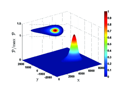
4.1 FADAE in two dimensions
Here we consider the two dimensional FSDAE which is not only of theoretical significance, but also potential application value [79, 80, 81, 66]. For simplification, the bias of the system is only in direction and the equation reads
| (37) |
Here , , , and are constants. Taking double Fourier transforms, and , we get
| (38) |
Using convolution properties of Fourier transform, Eq. (38) yields
| (39) |
where is the non-symmetric Lévy stable distribution Eq. (12). Below we obtain four transport coefficients given in Eq. (37). In the language of the CTRW model, the displacement follows
| (40) |
where , , and are constants. In double Fourier spaces, and , we get
| (41) |
For the waiting time, we continue to utilize the fat-tailed power law distribution Eq. (4). Using Eq. (25) and the same arguments as before, we find
| (42) |
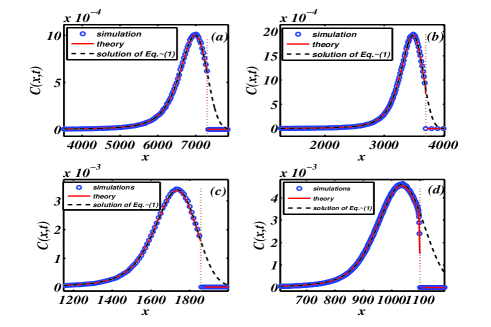
It can be seen that when the external force is only in the direction, the fat tail of the packet of spreading particle is with respect to . Note that the exact solution of Eq. (37) is Eq. (39), i.e., in the long time limit. What we want to stress is that when the bias is also in the direction, the fractional space operator with respect to should be added. See the solution of Eq. (37) in Fig. 3 and the marginal distribution in Fig. 4.

4.2 Propagator with the time-dependent bias and variance
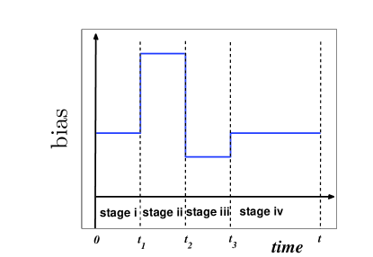
Motivated by [66], we consider the time-dependent bias and variance determined by four states. In some sense, assumptions are more closely aligned with the real-world spread of pollutants. This idea yields some interesting results, for example complex structure of breakthrough curves; see below. We suppose that the rapid injection of particles is done immediately after starting observing the process. In other words, the initial positions of all particles are . Here we simulate the particles consisting of four states: (i) after the injection of the particles at time , they undergo CTRW processes with a constant bias determined by in time interval (here is the mean of displacements), (ii) during the time interval we increase the force, namely replace the bias with for , (iii) we further decrease the bias to from time to , and (iv) finally we return to the state (i) from time ; see Fig. 5 for the statistics of the bias versus time. Here is a constant that controls the strength of the force. Let for states (i), (ii), and (iv), i.e., . While, for state (iii), we use . In particular, when , the bias of all states mentioned above is the same but the variance is still time-dependent. Note that the elapsed time of each state should be a bit long, otherwise one can find that the difference between them is not very large. In Fourier space, the initial condition satisfies . In view of the special expression of , for different states is as follows
| (43) |
with
| (44) |
| (45) |
and
| (46) |
Here is related to the number of states. Recall that . In calculations, the main idea is that the final position of each state is treated as the initial position of the next stage. The inverse Fourier transform of Eq. (43) yields
| (47) |
describing the positional distribution of the mentioned four states. Note that when , the solution Eq. (47) is the same as Eq. (21) or that of Eq. (3). Below, we use Eq. (47) to predict breakthrough curves [82].
4.3 Breakthrough curves
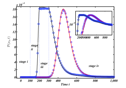
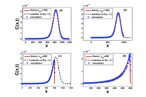
Contamination spreading, as one of the most crucial problems ranging from environment to agriculture, has attracted a lot of attention [80, 81, 66, 83, 84]. In real systems, how to quantity the contaminant transport is quite a challenge for researchers since the processes are so complex. In [66], Nissan, Dror and Berkowitz considered the spreading particle with changing conditions to illustrate the positive and negative effects of the ambient environment. It is no wonder that the changing force fields are quite common and vital in the real world. Theoretical predictions about breakthrough curves, which can be directly measured in experiments, were made using the CTRW particle tracking approach in [66]. While, here we choose Eq. (47) as a tool to describe breakthrough curves. The breakthrough curves are measured in the sense of the distribution, indicating the probability of particles being at at a specific time . The differences and similarities between the constant and the time-dependent force are quite interesting. When particles experience small disturbances or the total time of the first three states is short, the response of time-dependent force, calculated by the density of the position, is weak except for a ‘shift’. However, when we increase the total time of the first three states, the mentioned two cases exhibit great differences; see Fig. 6. Note that in our discussions the detection point is . Choosing the suitable detection point, i.e., , is a critical factor in observing the distinctive structure of the particle packet. For a short time , such as , it can be seen that since all the particles are on the way to the site pushed by the force and need more time to visit the position . As particles enter the second state, they are moving faster than the state (i) for , resulting in a rapid increase in the probability of the position. During the time interval , the disturbance and the variance are weak, leading to a more or less flat breakthrough curve. At the end of this state, there are still numerous particles being located at the left side of . In the last state, slowly tends to zero.
4.4 First passage time
So far we considered problems with free boundary conditions. The boundary conditions for fractional space diffusion equations are generally non-trivial. This is because fractional operators are non-local in space. Our approach to the problem is to use the subordination method, namely rely on Eqs. (8,10). The idea is as follows: We showed already that fluctuations of the number of renewals is given by Lévy statistics. We may think about the whole problem as a normal process, where is an operational time. Then this normal process is transformed from to the laboratory time . By normal process, we mean, for example, Brownian diffusion with advection in a finite domain, with reflecting or absorbing boundary conditions.
Here we consider as an example the case of the first passage time problem [85, 86, 87, 88, 89]. The first passage time serves as a significant tool for describing the time required by a particle to reach a specific point or an absorbing barrier. For standard diffusion this means that we use an absorbing boundary condition (see below). We will later show how to use subordination to obtain the solution for the anomalous process.
Before doing so we will briefly delve into the method of images. It was shown previously, that for Lévy flights the image method fails [90, 91, 92, 93]. However, in our case, we do not have any Lévy flight as an underlying process. Instead, we use fat-tailed distributions for waiting times. We will first show that the method of images generally fails in our case, however when the bias is weak it is a reasonable approximation. We will then turn to the more general solution using subordination.
4.4.1 Recap for the image method and it’s failure
Let us determine the first passage probability based on Eq. (3) for a diffusing particle that starts at . As mentioned, we use the image method and show that while it is generally not a good approximation, it works well when the bias is small. Here we assume that the absorbing boundary condition is and use to denote the concentration. Thus, when , we have . The most appealing approach, dealing with the absorbing boundary condition, is the method of images, which stems from electrostatics. As mentioned we will soon show, following Eq. (3), that this method does not work when the bias is not terribly small. In real space, the image method leads to [33, 85],
| (48) |
where the unknown parameter is defined below. Here denotes the positional distribution without absorbing condition, for example, below we use the solution of Eq. (3) to check the validity of the image method. It can be seen that the concentration is the difference between and with a weight determined by . Recall that vanish on , i.e., . Then obeys
Thus, we get with the image method
| (49) |
Consider the well-studied case of a particle undergoing normal diffusion (Eq. (3) with ) with an absorbing condition at . Thus, in the absence of the absorbing boundary condition follows Gaussian distribution
| (50) |
which leads to
| (51) |
according to Eq. (49). Note that in the general case is determined by , , and .
4.4.2 Subordinating the first passage problem
To solve this problem, we use a subordination technique that involves utilizing the method of images on the . Based on Eq. (8), the discrete form of follows
| (53) |
describing the subordinated process as a function of time . Here is the PDF of the number of the renewals given in Eq. (10) and is the solution of the ordinary Fokker-Planck equation
| (54) |
with the initial conditions and different boundary conditions, be specific, absorbing boundary condition at . The same approach can be used for other types of boundary conditions. Setting the absorbing condition on Eq. (54) and using the method of images for the solution of Eq. (54) yield
| (55) |
In the long time limit, the continuous form of Eq. (53) follows
| (56) |
Equation (56) is verified in Fig. 7 showing a perfect match. We now compare solution Eq. (56) and that of Eq. (3) with free boundary conditions. For that, the solution of Eq. (3) without absorbing condition was plotted by dashed black lines. As expected, when is much smaller than , is consistent with Eq. (3), i.e., the random particles are not affected by the absorbing condition, or most of particles have not yet reached the position near . In addition, when the bias is strong, Eq. (3) agrees with Eq. (56) for at least to the naked eye. Roughly speaking, this is because when the bias is strong, no particles are coming back. Thus, the absorbing condition under study loses its role. While, if approaches to and the bias is weak, Eq. (3) and Eq. (56) illustrate two different behaviors. See (d) in Fig. 7.
We further consider the first passage time using the survival probability. The survival probability describing the probability that the particles do not arrive on the position until the time reads
| (57) |
Let be the time to visit the position for the first time. Utilizing Eq. (57), the PDF of reads
| (58) |
| (59) |
with
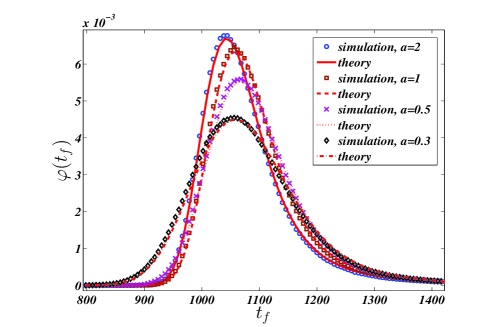
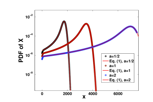
Here denotes the complementary error function, i.e., with error function . Eq. 59 is confirmed in Fig. (8) displaying a perfect match.
5 Three limiting laws of the positional distribution
Using Eq. (3), we derive three limiting laws that characterize the CTRW model under different conditions: when tends towards infinity, when approaches infinity, and when both and are constants. More exactly, these laws include the Lévy stable distribution showing the statistics when , Gaussian distribution in the context of , and a general expression that encompasses all values of and .
Taking Laplace transform on Eq. (29) with respect to , we have
| (60) |
We are interested in the statistics of in the long time limit, which means that both and go to zero in Eq. (60). Based on the above equation, the mentioned three laws will be discussed.
5.1 Lévy stable distribution when
Let , Eq. (60) yields
| (61) |
where we dropped the term due . The inverse Laplace-Fourier transforms of Eq. (61) lead to
| (62) |
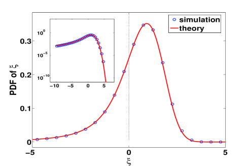
Integrating Eq. (62) from negative infinity to positive infinity implies that is a normalized density. See also the equivalent expression given in Eq. (19). This is illustrated in Fig. 9, where the PDF of with is plotted. Obviously, the PDF of is asymmetric with respect to , whose two tails show two different dynamic behaviors, namely the right-hand side of the tail tends to zero rapidly but the other one decays slowly like a power law; see the inset in Fig. 9. More precisely, based on Eq. (12), we get , being the same as the tail of the symmetric Lévy stable distribution, for . Thus, when , the integral diverges. This means that Eq. (62) does not give any information to the MSD, which will be discussed in Appendix B.
5.2 Gaussian distribution when
Note that Eq. (62) is independent of , and when is large, we expect this approximation to fail for a large but finite . Here we focus on the case when . As previously discussed, it is related to the linear response regime. In this limit, according to Eq. (60)
| (63) |
By inversion, using the shifting property of the inverse Fourier transform, yields the limiting distribution of . The scaling form of gives the Gaussian distribution with mean zero and variance one
| (64) |
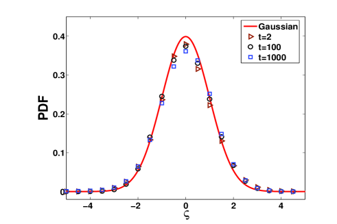
see Fig. 10. As expected, the simulations are consistent with the theoretical result Eq. (64) for a large . Recall that in Figs. 9 and 10, we used the same observation time , i.e., , but propagators are totally different (one is the Lévy stable law and the other is Gaussian distribution). It indicates that these laws are determined by the relationship between and . The current challenge is to determine a universal form that can represent both of the mentioned scalings.
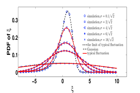
5.3 Typical fluctuations
We have discussed that under certain conditions the positional distribution follows Lévy stable distribution Eq. (62) or Gaussian distribution Eq. (64), determined by the relation between and . Therefore, it would be beneficial to acquire a universal law that applies to the aforementioned scenarios. Based on Eq. (60), we have
| (65) |
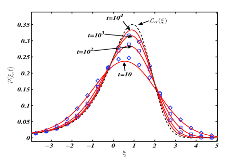
We denote Eq. (65), i.e., the solution of Eq. (3), as typical fluctuations describing the central of the positional distribution. As mentioned before, in the long time limit, Eq. (65) leads to the Lévy stable distribution Eq. (62). Figure 11 demonstrates the validity of Eq. (65) for various values of . For comparison, we also plot the solution Eq. (16) in Fig. 12. Eq. (16) agrees with Eq. (65) for large , it rapidly approaches zero as approaches zero, whereas Eq. (65) exhibits a cutoff at the tail. Therefore, the primary difference between the two equations lies in small values of .
To summarize, typical fluctuations Eq. (65), giving the information when , are valid for numerous , , and . One may wonder “why Eq. (65) is more useful than Eq. (19)?”. The reason is as follows: Mathematically, Eq. (19) is valid under the condition that . This implies that the observation time should be especially long, for example when is small and . While, Eq. (65) avoids this, this means that the condition reduces to .
6 Conclusion and discussion
In the context of the CTRW model, if the displacement follows a narrow distribution with a non-zero mean and the waiting time has an infinite mean, the fractional operator of the diffusion equation is linked to the Riemann-Liouville time derivative, as discussed in Refs. [4, 33]. However, nearly two decades later, the fractional-space advection-diffusion equation was developed for situations in which waiting times possess a finite mean and an infinite variance, together with the mentioned displacements [53]. As an extension of work [53], here we demonstrated further evidence of Eq. (3), gave more applications, and showed limiting laws of the kinetic equation, through our in-depth explanations. At the same time, theoretical predictions are checked by simulations of the CTRW model.
An issue here is that for Lévy flights, with a fat-tailed distribution of jump lengths, the method of images was shown to lead to wrong results, due to the non-local behavior [90, 91, 92]. One may wonder, whether or not the method of images will work for our process which does not include any fat-tailed jump length distribution. We show that generally, it does not work, unless for the case when the bias is small, then the image method is a valid approximation. For that, a subordination method was used. This method holds in general beyond the first passage problem, and it is also very different if compared to the subordination method used for . In practice we use the image method on the conditional probability , instead of the positional distribution . In particular, for a free particle, we assume Eq. (54) has a free boundary condition. In that sense, Eq. (55) reduces to given in Eq. (9). The mentioned strategy can also be extended to a much more general case, for example, the diffusion of particles on a finite domain. For applications, we also discussed the two-dimensional diffusion equation and breakthrough through curves with time-dependent bias and variance.
We demonstrated that the solution of Eq. (3) is obtained by convolving the Gaussian distribution with the Lévy stable distribution, see Eq. (65). Here we denote the solution of Eq. (3) as typical fluctuations of CTRW describing a wide range of , , and . In the language of the biased CTRW, the Lévy stable distribution stems from the PDF of the number of renewals, and the Gaussian distribution comes from the conditional distribution . When the bias is strong, i.e., , the diffusion term in Eq. (3) can be ignored and the solution is an asymmetric Lévy stable distribution Eq. (62). For the CTRW model, this limit is achieved when the ratio is finite and or with a finite . On the contrary, when , the spreading packet follows Gaussian distribution. It indicates that when , the well-known Eq. (62) is not useful unless is extremely long. Furthermore, we provide a parameter, denoted as , in Eq. (20) to characterize the convergence.
There are still unanswered questions that require addressing. For example, in the simulation of particle trajectories, generally, we first generate waiting times and displacements. Then, upon the completion of the total observation time, denoted as , we obtain positional statistics. However, when the observation time is long and the number of realizations is large, such as , running codes may require several days to complete. The problem now is whether we can generate particle statistics based on Eq. (21). More precisely, we first generate a variable drawn from the Lévy stable distribution , and then use it to generate the position at time according to a Gaussian distribution. This method seems fine if we are only interested in the positional distribution, but it fails as expected when we focus on the MSD. Solving this problem, i.e. formulating Langevin paths, is a matter that will be considered in the future.
Acknowledgments
W.W. is supported by the National Natural Science Foundation of China under Grant No. 12105243 and the Zhejiang Province Natural Science Foundation LQA. E.B. acknowledges the Israel Science Foundations grant .
Appendix A Additional discussions on Fig. 2
From simulations of typical fluctuations in Fig. 2, we can see that
we have defined by Eq. (20) with , , and . In the particular case , from Eq. (20) we get a small , this is the reason why Eq. (16) tends to the limit theorem Eq. (19) or (62) as shown by the black dashed line in Fig. 2.
However, when , and then , which is certainly not a small number if compared with . Thus even though the average of renewals , we cannot say that
the limit of is reached, and indeed, just as the bottom line in Fig. 2 shows, we see for this case nearly Gaussian behavior. For asymmetry breaking properties, one choice is to consider . This means that when , the corresponding density is asymmetric. While, for a large , the opposite situation emerges.
Appendix B Fractional moments
As mentioned before, Eq. (3) fails to estimate MSD of the CTRW model. Recently, we give a way to compute the MSD using infinite densities [68]. Here we show that infinite density frameworks can also used to calculate the fractional moments in an asymptotic sense. For the sake of completeness, first let us concentrate on the variance of the walk’s displacement, called MSD, which is a measure of the deviation of the position of the particle with respect to the position over time. Suppose that is the initial position of particles and is the number of renewals between and . Thus, the first and the second order moment of the position are given by
| (66) |
and
| (67) |
respectively. Here denotes the displacement of the particle in the -th jump and describes the average over . Therefore, the variance is
| (68) |
where we assumed that are IID random variables, and and correspond to the first and the second order moments of , respectively. Let us take the step length distribution as Eq. (6), thus we have and . To obtain , we need to calculate the first and the second moments of . Using the previous results given in Ref. [59], we have
| (69) |
and
| (70) |
Utilizing Eqs. (69) and (70), Eq. (68) gives
| (71) |
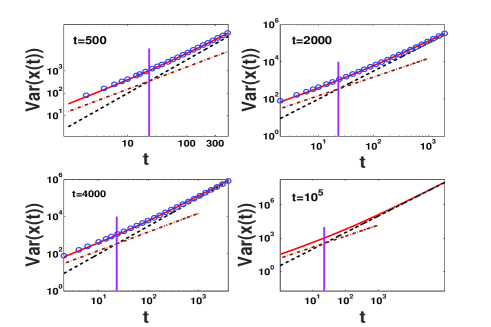
which is plotted in Fig. 13. The term becomes the leading term of as we increase of the observation time ; See also discussions in Ref. [68]. When the observation time is not very large, the linear term wins since the spreading packet nearly follows Gaussian distribution; see the dash-dotted line in Fig. 13. For a fixed observation time , we can find an interesting phenomenon depicting the competition between anomalous diffusion and normal diffusion, which is determined by , , and . According to Eq. (71), the transition point is
| (72) |
see the magenta vertical lines in Fig. 13. When , goes to infinity. It indicates that when the bias is weak, the process needs a long observation time to exhibit anomalous behaviors. On the other hand, when approaches infinity, the value of tends to zero, causing the transition from normal diffusion to anomalous diffusion rapidly.
When , the corresponding moment is
| (73) |
Using Eq. (8), the integer order moments are easy to get. Then substituting them into Eq. (73) gives
| (74) |
Now the calculation of is transformed into the moments of the number of renewals. After some simple arithmetics, we have
| (75) |
Our next step is to explore order absolute moments of , defined by
| (76) |
with . Let us start from the calculation of low order moments, i.e., . The low order moments can be obtained by the limit of typical fluctuations Eq. (19), which reads
| (77) |
When , the integral is a finite number which can be evaluated by the asymptotic behaviors of Lévy distribution . We can check that for , is always sublinear in . Here we would like to consider two special cases: for , the zeroth moment of the variable is, evidently, one; the other case is the Gaussian limit, the linear time dependence of the MSD is recovered, namely . For , Eq. (77) diverges. It indicates that the normalized density Eq. (19) can not give a valid prediction for high order moments; see Eq. (68).
Now we consider high-order moments. As mentioned before, for this case, typical fluctuations does not work. In [68], we demonstrate the existence of an additional limiting law when the second time scale is taken into account. This law, denoted as Eq. (78), characterizes the scaling behavior when is of the order of . Namely, the density of is
| (78) |
with . See numerical simulations and discussions in Ref. [68].
As mentioned, this situation for is especially important in physical and biological experiments [94, 4]. After rescaling Eq. (78) by , it can be seen that is integrable with respect to this non-normalized state. So this can be used to get high order moments, i.e.,
| (79) |
This demonstrates that, in the long time regime, the asymptotic distribution of is broad with a slowly decaying tail; see Eq. (78). Note that when is not sufficient large, the correction term is necessary to be added since the packet of particles is Gaussian; see left top panel in Fig. 13.
Appendix C Plot of concentration with a weak bias
We plot Eq. (52) obtained from the image method for a weak bias; see Fig. 14. For this case, the asymmetric term loses its role and the process is nearly normal. As mentioned in the main text, if the bias is strong, Eq. (52) breaks down.
References
- [1] Shlesinger M F 1974 Asymptotic solutions of continuous-time random walks. J. Stat. Phys. 10 421–434
- [2] Montroll E W, Weiss G H 1965 Random walks on lattices. II. J. Math. Phys. 6 167–181
- [3] Bouchaud J P, Georges A 1990 Anomalous diffusion in disordered media: statistical mechanisms, models and physical applications. Phys. Rep. 195 127–293
- [4] Metzler R, Klafter J 2000 The random walk’s guide to anomalous diffusion: a fractional dynamics approach. Phys. Rep. 339 1–77
- [5] Chaudhuri P, Berthier L, Kob W 2007 Universal nature of particle displacements close to glass and jamming transitions. Phys. Rev. Lett. 99 060604
- [6] Weigel A V, Simon B, Tamkun M M, Krapf D 2011 Ergodic and nonergodic processes coexist in the plasma membrane as observed by single-molecule tracking. PNAS 108 6438—6443
- [7] Meroz Y, Sokolov I M 2015 A toolbox for determining subdiffusive mechanisms. Physics Reports 573 1–29
- [8] Höfling F, Franosch T 2013 Anomalous transport in the crowded world of biological cells. Rep. Prog. Phys. 76 046602
- [9] Gradenigo G, Bertin E, Biroli G 2016 Field-induced superdiffusion and dynamical heterogeneity. Phys. Rev. E 93 060105
- [10] Kutner R, Masoliver J 2017 The continuous time random walk, still trendy: fifty-year history, state of art and outlook. Eur. Phys. J. B 90 50
- [11] Comolli A, Dentz M 2018 Impact of diffusive motion on anomalous dispersion in structured disordered media: From correlated Lévy flights to continuous time random walks. Phys. Rev. E 97 052146
- [12] Barkai E, Burov S 2020 Packets of diffusing particles exhibit universal exponential tails. Phys. Rev. Lett. 124 060603
- [13] Michelitsch T M, Polito F, Riascos A P 2020 Biased continuous-time random walks with Mittag-Leffler jumps. Fractal and Fractional 4 51
- [14] Vot F L, Abad E, Metzler R, Yuste S B 2020 Continuous time random walk in a velocity field: role of domain growth, Galilei-invariant advection-diffusion, and kinetics of particle mixing. New J. Phys. 22 073048
- [15] Wang W, Barkai E, Burov S 2020 Large deviations for continuous time random walks. Entropy 22 697
- [16] Pacheco-Pozo A, Sokolov I M 2021 Large deviations in continuous-time random walks. Phys. Rev. E 103 042116
- [17] Liu J, Zhu P, Bao J D, Chen X 2022 Strong anomalous diffusive behaviors of the two-state random walk process. Phys. Rev. E 105 014122
- [18] Michelitsch T M, Polito F, Riascos A P 2022 Asymmetric random walks with bias generated by discrete-time counting processes. Commun. Nonlinear Sci. Numer. Simul. 109 106121
- [19] Burov S, Wang W, Barkai E Exponential tails and asymmetry relations for the spread of biased random walks. ArXiv:2209.03410
- [20] Vitali S, Paradisi P, Pagnini G 2022 Anomalous diffusion originated by two markovian hopping-trap mechanisms. J. Phys. A: Math. Theor. 55 224012
- [21] Dentz M, Kirchner J W, Zehe E, Berkowitz B 2023 The role of anomalous transport in long-term, stream water chemistry variability. Geophys. Res. Lett. 50 e2023GL104207
- [22] Scher H, Montroll E W 1975 Anomalous transit-time dispersion in amorphous solids. Phys. Rev. B 12 2455–2477
- [23] David S A, Valentim C A, Debbouche A 2022 Fractional modeling applied to the dynamics of the action potential in cardiac tissue. Fractal Fract. 6
- [24] Deng W 2009 Finite element method for the space and time fractional Fokker-Planck equation. SIAM J. Numer. Anal. 47 204–226
- [25] Sylvain T T A, Patrice E A, Marie E E J, Pierre O A, Hubert B B G 2022 A unified three-dimensional extended fractional analytical solution for air pollutants dispersion. Fractals 30 2250065
- [26] Suleiman K, Song Q, Zhang X, Liu S, Zheng L 2022 Anomalous diffusion in a circular comb with external velocity field. Chaos, Solitons & Fractals 155 111742
- [27] Yan Z 2022 New integrable multi-Lévy-index and mixed fractional nonlinear soliton hierarchies. Chaos, Solitons & Fractals 164 112758
- [28] Evangelista L R, Lenzi E K 2023 Fractional Anomalous Diffusion, 189–236 (Cham: Springer International Publishing)
- [29] Tang Y, Gharari F, Arias-Calluari K, Alonso-Marroquin F, Najafi M N 2023 Variable order porous media equations: Application on modeling the S&P500 and bitcoin price return. ArXiv:2309.04206
- [30] Uchaikin V, Sibatov R 2013 Fractional Kinetics in Solids (Singapore: World Scientific)
- [31] Eraso-Hernandez L, Riascos A, Michelitsch T, Wang-Michelitsch J 2021 Random walks on networks with preferential cumulative damage: Generation of bias and aging. J. Stat. Mech: Theory Exp. 2021 063401
- [32] Metzler R, Barkai E, Klafter J 1999 Anomalous diffusion and relaxation close to thermal equilibrium: a fractional Fokker-Planck equation approach. Phys. Rev. Lett. 82 3563–3567
- [33] Barkai E 2001 Fractional Fokker-Planck equation, solution, and application. Phys. Rev. E 63 046118
- [34] Oldham K B, Spanier J 1974 The Fractional Calculus (Academic Press, New York)
- [35] Benson D A, Wheatcraft S W, Meerschaert M M 2000 The fractional-order governing equation of Lévy motion. Water Resour. Res. 36 1413–1423
- [36] Samko S G, Kilbas A A, Marichev O I 1993 Fractional integrals and derivatives (Gordon and Breach Science Publishers, Yverdon)
- [37] Podlubny I 1999 Fractional Differential Equations (Academic Press, Inc., San Diego)
- [38] Meerschaert M M, Sikorskii A 2012 Stochastic Models for Fractional Calculus, vol. 43 of De Gruyter Studies in Mathematics (Walter de Gruyter & Co., Berlin)
- [39] Estrada-Rodriguez G, Gimperlein H, Painter K J, Stocek J 2019 Space-time fractional diffusion in cell movement models with delay. Math. Models Methods Appl. Sci. 29 65–88
- [40] Zheng X, Wang H 2020 An error estimate of a numerical approximation to a hidden-memory variable-order space-time fractional diffusion equation. SIAM J. Numer. Anal. 58 2492–2514
- [41] Hufnagel L, Brockmann D, Geisel T 2004 Forecast and control of epidemics in a globalized world. PNAS 101 15124–15129
- [42] Lomholt M A, Ambjörnsson T, Metzler R 2005 Optimal target search on a fast-folding polymer chain with volume exchange. Phys. Rev. Lett. 95 260603
- [43] Brockmann D, Hufnagel L, Geisel T 2006 The scaling laws of human travel. Nature 439 462–465
- [44] Benson D A, Schumer R, Meerschaert M M, Wheatcraft S W 2001 Fractional dispersion, Lévy motion, and the MADE tracer tests. Transp. Porous Media 42 211–240
- [45] Zaburdaev V, Denisov S, Klafter J 2015 Lévy walks. Rev. Mod. Phys. 87 483–530
- [46] Zhang Y, Meerschaert M M, Neupauer R M 2016 Backward fractional advection dispersion model for contaminant source prediction. Water Resour. Res. 52 2462–2473
- [47] Guo Y, Wang L 2021 Heat current flows across an interface in two-dimensional lattices. Phys. Rev. E 103 052141
- [48] Sin C S 2023 Cauchy problem for fractional advection-diffusion-asymmetry equations. Results in Mathematics 78 111
- [49] Saichev A I, Zaslavsky G M 1997 Fractional kinetic equations: solutions and applications. Chaos 7 753–764
- [50] Gorenflo R, Mainardi F, Vivoli A 2007 Continuous-time random walk and parametric subordination in fractional diffusion. Chaos Solitons Fractals 34 87–103
- [51] Weron K, Jurlewicz A, Magdziarz M, Weron A, Trzmiel J 2010 Overshooting and undershooting subordination scenario for fractional two-power-law relaxation responses. Phys. Rev. E 81 041123
- [52] Dybiec B, Gudowska-Nowak E 2010 Subordinated diffusion and continuous time random walk asymptotics. Chaos: An Interdisciplinary Journal of Nonlinear Science 20 043129
- [53] Wang W, Barkai E 2020 Fractional advection-diffusion-asymmetry equation. Phys. Rev. Lett. 125 240606
- [54] Chechkin A, Sokolov I M 2021 Relation between generalized diffusion equations and subordination schemes. Phys. Rev. E 103 032133
- [55] Zhou T, Trajanovski P, Xu P, Deng W, Sandev T, Kocarev L 2022 Generalized diffusion and random search processes. J. Stat. Mech.: Theory Exp. 2022 093201
- [56] Wang X, Chen Y 2022 Ergodic property of random diffusivity system with trapping events. Phys. Rev. E 105 014106
- [57] Defaveri L, dos Santos M A F, Kessler D A, Barkai E, Anteneodo C 2023 Non-normalizable quasiequilibrium states under fractional dynamics. Phys. Rev. E 108 024133
- [58] Berkowitz B, Klafter J, Metzler R, Scher H 2002 Physical pictures of transport in heterogeneous media: Advection-dispersion, random-walk, and fractional derivative formulations. Water Resour. Res. 38 9
- [59] Godrèche C, Luck J M 2001 Statistics of the occupation time of renewal processes. J. Stat. Phys. 104 489–524
- [60] Wang W, Schulz J H P, Deng W H, Barkai E 2018 Renewal theory with fat-tailed distributed sojourn times: Typical versus rare. Phys. Rev. E 98 042139
- [61] Metzler R, Jeon J H, Cherstvy A G, Barkai E 2014 Anomalous diffusion models and their properties: Non-stationarity, non-ergodicity, and ageing at the centenary of single particle tracking. Phys. Chem. Chem. Phys. 16 24128–24164
- [62] Margolin G, Berkowitz B 2002 Spatial behavior of anomalous transport. Phys. Rev. E 65 031101
- [63] Levy M, Berkowitz B 2003 Measurement and analysis of non-Fickian dispersion in heterogeneous porous media. J. Contam. Hydrol. 64 203–226
- [64] Schroer C F E, Heuer A 2013 Anomalous diffusion of driven particles in supercooled liquids. Phys. Rev. Lett. 110 067801
- [65] Luo L, Tang L H 2015 Sample-dependent first-passage-time distribution in a disordered medium. Phys. Rev. E 92 042137
- [66] Nissan A, Dror I, Berkowitz B 2017 Time-dependent velocity-field controls on anomalous chemical transport in porous media. Water Resour. Res. 53 3760–3769
- [67] Vezzani A, Barkai E, Burioni R 2019 Single-big-jump principle in physical modeling. Phys. Rev. E 100 012108
- [68] Wang W, Vezzani A, Burioni R, Barkai E 2019 Transport in disordered systems: The single big jump approach. Phys. Rev. Res. 1 033172
- [69] Zhang C, Hu Y, Liu J 2022 Correlated continuous-time random walk with stochastic resetting. J. Stat. Mech: Theory Exp. 2022 093205
- [70] Fogedby H C 1994 Langevin equations for continuous time Lévy flights. Phys. Rev. E 50 1657–1660
- [71] Magdziarz M, Weron A, Weron K 2007 Fractional Fokker-Planck dynamics: Stochastic representation and computer simulation. Phys. Rev. E 75 016708
- [72] Fedotov S, Han D 2023 Population heterogeneity in the fractional master equation, ensemble self-reinforcement, and strong memory effects. Phys. Rev. E 107 034115
- [73] Kotulski M 1995 Asymptotic distributions of continuous-time random walks: A probabilistic approach. J. Stat. Phys. 81 777–792
- [74] Burioni R, Gradenigo G, Sarracino A, Vezzani A, Vulpiani A 2013 Rare events and scaling properties in field-induced anomalous dynamics. J. Stat. Mech. Theory Exp. 2013 P09022
- [75] Metzler R, Barkai E, Klafter J 1999 Deriving fractional Fokker-Planck equations from a generalised master equation. EPL 46 431–436
- [76] Deng W, Hou R, Wang W, Xu P 2020 Modeling Anomalous Diffusion: From Statistics to Mathematics (Singapore: World Scientific)
- [77] Zhang X, Crawford J W, Deeks L K, Stutter M I, Bengough A G, Young I M 2005 A mass balance based numerical method for the fractional advection-dispersion equation: Theory and application. Water Resour. Res. 41
- [78] Metzler R, Rajyaguru A, Berkowitz B 2022 Modelling anomalous diffusion in semi-infinite disordered systems and porous media. New J. Phys. 24 123004
- [79] Berkowitz B, Kosakowski G, Margolin G, Scher H 2001 Application of continuous time random walk theory to tracer test measurements in fractured and heterogeneous porous media. Ground Water 39 593–604
- [80] Berkowitz B, Cortis A, Dentz M, Scher H 2006 Modeling non-Fickian transport in geological formations as a continuous time random walk. Rev. Geophys. 44
- [81] Berkowitz B, Scher H 2009 Exploring the nature of non-Fickian transport in laboratory experiments. Adv. Water Resour. 32 750–755
- [82] Cortis A, Berkowitz B 2004 Anomalous transport in “Classical” soil and sand columns. Soil Sci. Soc. Am. J. 68 1539–1548
- [83] de Moraes R, Ozelim L, Cavalcante A 2022 Generalized skewed model for spatial-fractional advective–dispersive phenomena. Sustainability 14
- [84] Doerries T J, Chechkin A V, Schumer R, Metzler R 2022 Rate equations, spatial moments, and concentration profiles for mobile-immobile models with power-law and mixed waiting time distributions. Phys. Rev. E 105 014105
- [85] Redner S 2001 A Guide to First-Passage Processes (Cambridge University Press, Cambridge)
- [86] Metzler R, Chechkin A V, Klafter J 2012 Lévy Statistics and Anomalous Transport: Lévy Flights and Subdiffusion, 1724–1745 (New York: Springer)
- [87] Wardak A 2020 First passage leapovers of Lévy flights and the proper formulation of absorbing boundary conditions. J. Phys. A: Math. Theor. 53 375001
- [88] Zan W, Xu Y, Metzler R, Kurths J 2021 First-passage problem for stochastic differential equations with combined parametric gaussian and Lévy white noises via path integral method. J. Comput. Phys. 435 110264
- [89] Höll M, Nissan A, Berkowitz B, Barkai E ArXiv:2208.10262
- [90] Chechkin A V, Metzler R, Gonchar V Y, Klafter J, Tanatarov L V 2003 First passage and arrival time densities for Lévy flights and the failure of the method of images. J. Phys. A: Math. Gen. 36 L537
- [91] Sokolov I M, Metzler R 2004 Non-uniqueness of the first passage time density of Lévy random processes. J. Phys. A: Math. Gen. 37 L609–L615
- [92] Palyulin V V, Blackburn G, Lomholt M A, Watkins N W, Metzler R, Klages R, Chechkin A V 2019 First passage and first hitting times of Lévy flights and Lévy walks. New J. Phys. 21 103028
- [93] Padash A, Chechkin A V, Dybiec B, Pavlyukevich I, Shokri B, Metzler R 2019 First-passage properties of asymmetric Lévy flights. J. Phys. A: Math. Theor. 52 454004
- [94] Barkai E, Garini Y, Metzler R 2012 Strange kinetics of single molecules in living cells. Phys. Today 65 29–35