Augmented quantization: a general approach to mixture models

Abstract

The estimation of mixture models is a key to understanding and visualizing the distribution of multivariate data. Most approaches to learning mixture models involve likelihoods and are not adapted to distributions with finite support or without a well-defined density function.

This study proposes the Augmented Quantization method, which is a reformulation of the classical quantization problem but which uses the $p$-Wasserstein distance. This metric can be computed in very general distribution spaces, in particular with varying supports. The clustering interpretation of quantization is revisited with distances between distributions. The Augmented Quantization algorithm can handle mixtures of discrete and continuous measures, with finite or infinite supports. Each step of the algorithm is supported by local minimizations of the generalized quantization error. The performance of Augmented Quantization is first demonstrated through analytical toy problems. Subsequently, it is applied to a practical case study involving river flooding, wherein mixtures of Dirac and uniform distributions are built in the input space, enabling the identification of the most influential variables.

1 Introduction

Quantization methods classically provide discrete representations of continuous distributions ([9]). Quantization is a key component of digitalization in signal processing ([17]) and, more generally, it can be employed as a clustering technique to approximate continuous random variables with a Dirac mixture ([20]). This representation is useful when describing continuous phenomena with a finite number of prototype elements. Discrete approximations to random variables are classically obtained by minimizing a Maximum Mean Discrepancy ([26]) or as centroids of Voronoi cells in the K-means clustering ([11]).

However, when approximating a random variable, it may be desirable to come up with a representation that is more complex than a discrete distribution. Mixture models are relevant in this case. They aim to identify subpopulations in a sample that arise from a common distribution but with different parameters ([1]). Gaussian mixture models are probably the most popular and highlight normally distributed subgroups. Mixture models, which can be seen as clustering methods, expand conventional quantization by allowing the use of any distribution in place of the Dirac measure. The mixture is learned with the Expectation-Maximization (EM) algorithm ([6]), which performs a probabilistic assignment of each point to a cluster by the computation of likelihoods, followed by the estimation of the cluster parameters by likelihood maximization. In certain applications, it is necessary to study specific distributions mixes. For example, in the flooding case study (cf. Section 7) where the objective is to gain insights into the influence of variables in relation to specific flood spatial patterns, we investigate subdistributions that consist either of a Dirac measure at a specific value or a uniform distribution with its support. Here, larger supports denote less influential variables.

Learning very general distributions is not easy. Distributions such as the uniform or the Dirac measure overlook points out of their supports and processing them through likelihoods and such direct functionals of their density will fail. Appendix A illustrates this problem with uniform distributions whose supports include all the points, even the obvious outliers. Density is not even defined when it comes to Dirac mixtures or to distributions with singular components. One possible remedy is to work with zero-inflated beta distributions ([2]), but they remain less general and harder to interpret than the well-known uniform, Dirac, or Gaussian distributions.

Thus, one objective of this article is to establish a framework for learning mixtures of general distributions. Our approach is based on computing the $p$-Wasserstein distance between two probability measures, $\mu$ and $\nu$, on a space $\mathcal{X}$, without strong restrictions on them ([27]). In particular, the $p$-Wasserstein distance is defined between measures that do not have the same support or when one is discrete and the other continuous. The $p$-Wasserstein distance is defined as follows:

$$\mathcal{W}(\mu,\nu)=\underset{\pi\in\bm{\Pi}(\mu,\nu)}{\mathrm{inf}}\left(\int_{\mathcal{X}\times\mathcal{X}}\lVert x-x^{\prime}\lVert^{p}\pi(dx,dx^{\prime})\right)^{\frac{1}{p}},$$

where $\bm{\Pi}(\mu,\nu)$ is the set of all the joint probability measures on $\mathcal{X}\times\mathcal{X}$ whose marginals are $\mu$ and $\nu$ on the first and second factors, respectively. This metric represents the optimal transport cost between the two measures and appears highly relevant in our context of approximation of a set of points by a general mixture.

However, finding the best mixture of $\ell$ different distributions (for a given $\ell\in\mathbb{N}$) is not straightforward, as calculating the weights and parameters of the distributions implies minimizing $p$-Wasserstein distances which are non-convex optimization problems ([13]). In addition, learning mixtures of distributions generates problems with many variables. For instance, a mixture of $4$ Dirac measures in $4$ dimensions is described by 20 variables.

Clustering approaches like K-means are popular in such high-dimensional situations. They reduce the size of the optimization problem by decomposing it cluster by cluster. Clustering also facilitates the interpretation of the results. Our method, that we call Augmented Quantization (AQ), is based on the classical K-means, generalized to handle various types of distributions using the $p$-Wasserstein distance.

The paper is structured as follows. The problem is formulated and a path towards Augmented Quantization is sketched in Section 2. Elements of analysis of Augmented Quantization are given in Section 3 followed, in Section 4, by a description of the implementation steps of the algorithm. In Section 5, the method is applied to several toy problems and compared to existing approaches, while in Section 7, it is applied to a study of real floodings. Finally, Section 8 summarizes the main results and proposes extensions to the method.

2 Augmented quantization

2.1 Problem formulation

The objective of the study conducted here is to build a very general mixture model that approximates the (unknown) underlying distribution of a (known) sample $(x_{i})_{i=1}^{n}\in\mathcal{X}^{n}$ with $\mathcal{X}\subset\mathbb{R}^{m}$.

The components of the mixture, called representatives, will be seen as probability measures on $\mathcal{X}$. They belong to a given family of probability measures which is not necessarily parametric. More precisely, we consider $\ell\in\mathbb{N}^{\star}$ representatives named through their tag taken in $\mathcal{J}=\{1,\dots,\ell\}$. Let $\mathcal{R}$ be a family of probability measures, the objective is approximate the distribution of $(x_{i})_{i=1}^{n}$ by the mixture $R_{J}$ such that

• $R_{J}=\sum_{j\in\mathcal{J}}\mathbb{P}(J=j)R_{j}$ ,

• $R_{j}\in\mathcal{R},\quad j\in\mathcal{J}$  ,

• $J$ a discrete random variable independent of $(R_{1},\dots,R_{\ell})$ with weights $p_{j}=P(J=j)$, $j\in\mathcal{J}$.

It is important to note that this representation is not necessarily unique, the identifiability of the problem depends on the family $\mathcal{R}$ ([28]). For instance, a mixture of the measures associated to $\mathcal{U}(0.5,1)$ and $\mathcal{U}(0,1)$ with weights $0.5$ on one hand, and a mixture of the measures associated to $\mathcal{U}(0,0.5)$ and $\mathcal{U}(0.5,1)$ with respective weights $0.25$ and $0.75$ on the other hand, are identical.

Augmented quantization, as the name indicates, generalizes the traditional quantization method and the accompanying K-means clustering. Let us first recall the basics of K-means. In K-means, the representatives are Dirac measures located at $\gamma$, $\mathcal{R}=\{\delta_{\gamma},\gamma\in\mathcal{X}\}.$ For a given set of representatives $\bm{R}=(R_{1},\dots,R_{\ell})=(\delta_{\gamma_{1}},\dots,\delta_{\gamma_{\ell}})\in\mathcal{R}^{\ell},$ the associated clusters are $\bm{C}=(C_{1},\dots,C_{\ell})$ with $C_{j}=\{x\in(x_{i})_{i=1}^{n}\,:\;j=\underset{i\in\mathcal{J}}{\argmin}\lVert x-\gamma_{i}\lVert\},j\in\mathcal{J}.$ The objective is to minimize the quantization error,

$$\small\mathcal{E}_{p}(\gamma_{1},\dots,\gamma_{\ell}):=\left(\frac{1}{n}\sum_{i=1}^{n}\lVert x_{i}-\underset{\gamma\in\Gamma_{\ell}}{\argmin}\lVert x_{i}-\gamma\lVert\lVert^{p}\right)^{\frac{1}{p}}\leavevmode\nobreak\ .$$ (1)

We now generalize the quantization error by replacing the Euclidean distance with a $p$-Wasserstein metric which, it turns, allows to rewrite the quantization error for any representatives $\bm{R}$ and associated clusters $\bm{C}$:

$$\mathcal{E}_{p}(\bm{C},\bm{R}):=\left(\sum_{j=1}^{\ell}\frac{\mathrm{card}\left(C_{j}\right)}{n}\mathcal{W}_{p}(C_{j},R_{j})^{p}\right)^{\frac{1}{p}},$$ (2)

where $\mathcal{W}_{p}(C_{j},R_{j})$ is the $p$-Wasserstein distance ([21]) between the empirical probability measure associated to $C_{j}$ and the measure $R_{j}$.

The traditional quantization error (1) is recovered from the general error 2 by limiting the representatives to Dirac measures and defining the clusters as nearest neighbors to the Dirac locations $\gamma_{i}\leavevmode\nobreak\ ,\leavevmode\nobreak\ i=1,\ldots,\ell$. The general clusters $C_{j}\leavevmode\nobreak\ ,\leavevmode\nobreak\ j=1,\ldots,\ell$ of Equation 2 form a partition of the samples $(x_{i})_{i=1}^{n}$. We will soon see how to define them.

2.2 From K-means to Augmented Quantization

Lloyd’s algorithm is one of the most popular implementation of K-means quantization ([7]). The method can be written as follows:

Input: $(\gamma_{1},\dots,\gamma_{\ell})\in\mathcal{X}^{\ell}$ , sample $(x_{i})_{i=1}^{n}$

while stopping criterion not met do

   FindC :  update the clusters,

   FindR :  update the representatives,

end while

Output:

• the membership discrete random variable $J$ with $\mathbb{P}(J=j)=\frac{\mathrm{card}\left(C_{j}\right)}{n},\quad j\in\mathcal{J}$

• the mixture $R_{J}=\sum_{j\in\mathcal{J}}\mathbb{P}(J=j)\delta_{\gamma_{j}}$

Algorithm 1 Lloyd’s algorithm

Algorithm 1 is not the standard description of Lloyd’s algorithm but an interpretation paving the way towards augmented quantization and the estimation of mixture distributions: the centroids $(\gamma_{1},\dots,\gamma_{\ell})$ are seen as representatives $(R_{1},\dots,R_{\ell})$ through the Dirac measures $\delta_{\gamma}$; the produced Voronoi cells are translated into a mixture distribution.

At each iteration, new clusters $\bm{C}=(C_{1},\dots,C_{\ell})$ are determined from the previously updated representatives (centroids in this case), and then new representatives $\bm{R}=(R_{1},\dots,R_{\ell})$ are computed from the new clusters. These operations reduces the quantization error. We refer to these two steps as $FindC$ and $FindR$. The stopping criterion is typically related to a very slight difference between the calculated representatives and those from the previous iteration.

The usual quantization is augmented by allowing representatives that belong to a predefined set of probability measures $\mathcal{R}$. In Augmented Quantization, $\mathcal{R}$ can still contain Dirac measures but it will typically include other measures. Each iteration alternates between $\bm{C}$ during $FindC$ and the mixture defined by $(\bm{R},J)$ during $FindR$. $FindC$ is now a function which partitions $(x_{i})_{i=1}^{n}$ into clusters based on a set of the representatives and the random membership variable $J$. $FindR$ is a function which generates a set of representatives from a partition of $(x_{i})_{i=1}^{n}$. Algorithm 2 is the skeleton of the Augmented Quantization algorithm.

Lloyd’s algorithm can be seen as descent algorithm applied to the minimization of the quantization error (Equation (1)). It converges to a stationary point which may not even be a local optimum ([22]). Although Lloyd’s algorithm converges generally to stationary points that have a satisfactory quantization error, Appendix B illustrates that its generalization to continuous distributions does not lead to a quantization error sufficiently close to the global optimum. To overcome this limitation, an additional mechanism for exploring the space of mixture parameters is needed. To this aim, we propose a perturbation of the clusters called $Perturb()$, which takes place between $FindC$ and $FindR$.

Input: $\bm{R}=(R_{1},\dots,R_{\ell})\in\mathcal{R}^{\ell}$, samples $(x_{i})_{i=1}^{n}$

$J\in\mathcal{J}$ r.v. with $\mathbb{P}(J=j)=\frac{1}{\ell}$

$(R^{\star},C^{\star},\mathcal{E}^{\star})\leftarrow(\emptyset,\emptyset,+\infty)$

while stopping criterion not met do

   Update clusters: $\bm{C}\leftarrow FindC(\bm{R},J)$

   Perturb clusters: $\bm{C}\leftarrow Perturb(\bm{C})$

   Update mixture: $\bm{R}\leftarrow FindR(\bm{C})$, $J$ r.v. with $\mathbb{P}(J=j)=\frac{\mathrm{card}\left(C_{j}\right)}{n},\>j\in\mathcal{J}$

   Update the best configuration:

   if $\mathcal{E}_{p}(\bm{C},\bm{R})<\mathcal{E}^{\star}$ then $\mathcal{E}^{\star}\leftarrow\mathcal{E}\leavevmode\nobreak\ ,\leavevmode\nobreak\ \bm{C}^{\star}\leftarrow\bm{C}\leavevmode\nobreak\ ,\leavevmode\nobreak\ \bm{R}^{\star}\leftarrow\bm{R}\leavevmode\nobreak\ ,\leavevmode\nobreak\ J^{\star}\leftarrow J$

end while

Output:

• the membership discrete random variable $J^{\star}$ with $\mathbb{P}(J^{\star}=j)=\frac{\mathrm{card}\left(C_{j}^{\star}\right)}{n},\;j\in\mathcal{J}$

• the mixture $R_{J^{\star}}^{\star}$

Algorithm 2 Augmented Quantization algorithm

3 Definition and properties of quantization errors

Before describing in details the $FindC$, $Perturb$ and $FindR$ steps, some theoretical elements are provided that will be useful to explain our implementation choices.

3.1 Quantization and global errors

Let $\bm{R}=(R_{1},\dots,R_{\ell})$ be $\ell$ probability measures and $\bm{C}=(C_{1},\dots,C_{\ell})$ be $\ell$ disjoint clusters of points in $\mathcal{X}\subset\mathbb{R}^{d}$. Let us denote $n_{j}=\mathrm{card}\left(C_{j}\right)$ for $j\in\mathcal{J}$, and $n=\sum_{j=1}^{n}n_{j}$.

The quantization error between $\bm{C}$ and $\bm{R}$ is defined by

$$\mathcal{E}_{p}(\bm{C},\bm{R}):=\left(\sum_{j}^{\ell}\frac{n_{j}}{n}\mathcal{W}_{p}(C_{j},R_{j})^{p}\right)^{1/p}.$$ (3)

It should not be mistaken with the global error between $\bm{C}$ and $\bm{R}$, which is defined by

$$\epsilon_{p}(\bm{C},\bm{R}):=\mathcal{W}_{p}\left(\bigcup_{j=1}^{\ell}C_{j},R_{J}\right),$$ (4)

where $J\in\mathcal{J}$ is a random variable such that $\mathbb{P}(J=j)=\frac{n_{j}}{n}.$ The quantization error aggregates the local errors between the clusters and the representatives, while the global error characterizes the overall mixture.

The quantization error is a natural measure of clustering performance and clustering is a way to decompose the minimization of the global error. Such a decomposition is justified by Proposition 1, which shows that a low quantization error guarantees a low global error.

Proposition 1 (Global and quantization errors).

The global error between a clustering $\bm{C}$ and a set of representatives $\bm{R}$ is lower that the quantization error between them:

$$\epsilon_{p}(\bm{C},\bm{R}) =\mathcal{W}_{p}\left(\bigcup_{j=1}^{\ell}C_{j},R_{J}\right)$$

$$\leq\left(\sum_{j}^{\ell}\frac{n_{j}}{n}\mathcal{W}_{p}(C_{j},R_{j})^{p}\right)^{1/p}=\mathcal{E}_{p}(\bm{C},\bm{R})\leavevmode\nobreak\ .$$

The proof is provided in Appendix C.

3.2 Clustering error

For a given clustering $\bm{C}=(C_{1},\dots,C_{\ell})$, the optimal representatives can be calculated individually for each cluster. This optimization allows to introduce the notion of quantization error of a clustering.

Proposition 2 (Quantization error of a clustering).

Let $\bm{C}=(C_{1},\dots,C_{\ell})$ be $\ell$ clusters of points in $\mathcal{X}$ and the associated optimal representatives

$$\bm{R}^{\star}(\bm{C}):=\underset{\bm{R}\in\mathcal{R}^{\ell}}{\argmin}\>\mathcal{E}_{p}(\bm{C},\bm{R})\leavevmode\nobreak\ .$$

Then:

1. The optimal representatives can be optimized independently for each cluster,

   $$\begin{multlined}\bm{R}^{\star}(\bm{C})=(R^{\star}_{1}(C_{1}),\dots,R^{\star}_{\ell}(C_{\ell}))\\ \mathrm{where}\;R^{\star}_{j}(C_{j}):=\underset{r\in\mathcal{R}}{\argmin}\>\mathcal{W}_{p}(C_{j},r),\>j\in\mathcal{J}.\end{multlined}\bm{R}^{\star}(\bm{C})=(R^{\star}_{1}(C_{1}),\dots,R^{\star}_{\ell}(C_{\ell}))\\ \mathrm{where}\;R^{\star}_{j}(C_{j}):=\underset{r\in\mathcal{R}}{\argmin}\>\mathcal{W}_{p}(C_{j},r),\>j\in\mathcal{J}.$$

   This results trivially from the fact that $\mathcal{E}_{p}$ is a monotonic transformation of a sum of independent components.

2. The local error of a cluster $C_{j}$ is defined as the $p$-Wasserstein distance between $C$ and its optimal representative $R^{\star}_{j}(C_{j})$,

   $$w_{p}(C_{j}):=\mathcal{W}_{p}(C_{j},R^{\star}_{j}(C_{j}))=\underset{r\in\mathcal{R}}{\mathrm{min}}\>\mathcal{W}_{p}(C_{j},r)\leavevmode\nobreak\ .$$

3. The quantization error of a clustering $\bm{C}$ is the quantization error between $\bm{C}$ and $\bm{R}^{\star}(\bm{C})$, its associated optimal representatives,

   $$\mathcal{E}_{p}(\bm{C}):=\mathcal{E}_{p}(\bm{C},\bm{R}^{\star}(\bm{C}))=\underset{\bm{R}\in\mathcal{R}^{\ell}}{\mathrm{min}}\>\mathcal{E}_{p}(\bm{C},\bm{R})\leavevmode\nobreak\ .$$

4. The global error associated to a clustering $\bm{C}$ is lower than its quantization error,

   $$\epsilon_{p}(\bm{C})\leq\mathcal{E}_{p}(\bm{C})$$

   with $\epsilon_{p}(\bm{C})=\epsilon_{p}(\bm{C},\bm{R}^{\star}(\bm{C}))=\mathcal{W}_{p}(\bigcup_{j=1}^{\ell}C_{j},R^{\star}_{J}(C_{J}))$ and $\mathbb{P}(J=j)=\frac{n_{j}}{n},\>j\in\mathcal{J}$ . This follows directly from Proposition 1.

The above clustering error is based on a $p$-Wasserstein distance minimization in the space of probability measures $\mathcal{R}$. This problem is further addressed in Section 4.3 when seeking representatives from given clusters.

4 Algorithm steps

The steps of the Augmented Quantization algorithm can now be presented in details. We will explain how they contribute to reducing the quantization error which was discussed in Section 3.

4.1 Finding clusters from representatives

At this step, a mixture distribution $R_{J}$ is given through its $\ell$ representatives $\bm{R}=(R_{1},\dots,R_{\ell})$ and the associated membership random variable $J$ such that $P(J=j)=p_{j}\leavevmode\nobreak\ ,\leavevmode\nobreak\ j=1,\ldots,\ell$. Clustering is performed by, first, creating $N$ samples from the mixture distribution: the membership variable $j$ is sampled from $J$, and each point is drawn from $R_{j}$. Second, the data points are assigned to the cluster to which belongs the closest of the $N$ samples. Before returning to the algorithm, we provide a theoretical justification for it.

Let $(X_{i})_{i=1}^{n}\in\mathcal{X}^{n}$ be a random sample of the above $R_{J}$ mixture distribution. $(J_{i})_{i=1}^{N}$ are i.i.d. samples with the same distribution as $J$, and $(Y_{i})_{i=1}^{N}$ i.i.d. samples with $Y_{i}\sim R_{J_{i}},\>i=1,\dots,N.$ We define the following clustering,

$$\bm{C}^{\star}(R,J,n,N):=\Bigl{(}C^{\star}_{1}(R,J,n,N),\dots,C^{\star}_{\ell}(R,J,n,N)\Bigl{)}$$

with

$$C^{\star}_{j}(R,J,n,N):=\{X_{k}\;s.t.\;J_{I_{N}(X_{k})}=j\;,\;1\leq k\leq n\},$$

$$\text{and }\quad I_{N}(x):=\underset{i=1,\dots,N}{\argmin}{\mid\mid x-Y_{i}\mid\mid}\leavevmode\nobreak\ .$$

We work with general distributions that are combinations of continuous and discrete distributions,

$\mathcal{R}_{s}:=\{\beta_{\mathrm{c}}R_{\mathrm{c}}+\beta_{\mathrm{disc}}R_{\mathrm{disc}},R_{\mathrm{c}}\in\mathcal{R}_{\mathrm{c}},R_{\mathrm{disc}}\in\mathcal{R}_{\mathrm{disc}},\beta_{\mathrm{c}}+\beta_{\mathrm{disc}}=1\}$.

$\mathcal{R}_{\mathrm{c}}$ and $\mathcal{R}_{\mathrm{disc}}$ are the set of measures associated to almost everywhere continuous distributions with finite support, and, the set of measures associated to discrete distributions with finite support, respectively.

In the family of probability measures $R_{s}$, the above clustering is asymptotically consistent: the quantization error associated to this clustering is expected to tend to zero as $n$ and $N$ increase.

Proposition 3.

If $R_{j}\in\mathcal{R}_{s}$ for $j\in\mathcal{J}$ and $X_{i}\sim R_{J^{X}_{i}},\;i=1,\dots,n$ with $(J^{X}_{i})_{i=1}^{n}$ i.i.d. sample with same distribution as $J$, then

$$\underset{n,N\rightarrow+\infty}{lim}\mathbb{E}\left(\mathcal{W}_{p}(C^{\star}_{j}(R,J,n,N),R_{j})\right)=0,\quad j\in\mathcal{J}.$$

As a consequence,

$$\underset{n,N\rightarrow+\infty}{lim}\mathbb{E}\left(\mathcal{E}_{p}(\bm{C}^{\star}(R,J,n,N))\right)=0.$$

The proof along with further details about $\mathcal{R}_{s}$ are given in Appendix D.

The objective of the $FindC$ procedure is to associate a partition of a sample $(x_{i})_{i=1}^{n}$ to the representatives $\bm{R}$ with probabilistic weights defined by the random variable $J$. It is described in Algorithm 3.

Input: Sample $(x_{i})_{i=1}^{n}$, $\bm{R}=(R_{1},\dots,R_{\ell})$, $N$, $J$ r.v. $\in\mathcal{J}$

$C_{j}=\emptyset,\>j\in\mathcal{J}$

$(j_{i})_{i=1}^{N}$ N independent realizations of $J$

$(y_{i})_{i=1}^{N}$ N independent realizations, $y_{i}$ sampled with associated measure $R_{j_{i}}$

for $x\in(x_{i})_{i=1}^{n}$ do

   $I(x)\leftarrow\underset{i=1,\dots,N}{\argmin}{\mid\mid x-y_{i}\mid\mid}$

   $C_{j_{I(x)}}\leftarrow C_{j_{I(x)}}\cup x$

end for

Algorithm 3 $FindC$

Output: Partition $\bm{C}=(C_{1},\dots,C_{\ell})$

The $FindC$ algorithm is consistent in the sense of the above Proposition 3.

4.2 Perturb clusters

Once clusters are associated to representatives, the $Perturb$ step is required to explore the space of partitions of $(x_{i})_{i=1}^{n}$. Appendix B illustrates why such a step is important through the example of a mixture of two uniforms that, without perturbation, cannot be identified from a given, seemingly reasonable, starting clustering. Thus, a relevant cluster perturbation should be sufficiently exploratory. To increase convergence speed, we make it greedy by imposing a systematic decrease in quantization error.

Proposition 4 (Greedy cluster perturbation).

Let $\bm{C}=(C_{1},\dots,C_{\ell})$ be a clustering, and $G(\bm{C})$ a set of perturbations of this clustering such that $\bm{C}\subset G(\bm{C})$.

The greedy perturbation, $Perturb()$, is a function that yields a new clustering $\bm{C}^{\star}=Perturb(\bm{C})$ through $\bm{C}^{\star}:=\underset{\bm{C}^{\prime}\in G(\bm{C})}{\argmin}\mathcal{E}_{p}(\bm{C}^{\prime})$.

Trivially, $\mathcal{E}_{p}(\bm{C}^{\star})\leq\mathcal{E}_{p}(\bm{C})$.

The quantization error decrease comes from the inclusion of the current clustering in the set of perturbations. Here, we choose to perturb the clusters through the identification of the points contributing the most to the quantization error.

The need for a perturbation has also been described in classical K-means methods where it takes the form of a tuning of the initial centroids when restarting the algorithm ([3]).

Our cluster perturbation consists in, first, identifying the elements to move which defines the $split$ phase and, second, reassigning them to other clusters in what is the $merge$ phase.

$split$ phase

The clusters with the $\ell_{\mathrm{bin}}$ highest local errors $w_{p}$ will be split. Their indices make the $\mathrm{indexes_{bin}}$ list. During the $split$ phase, for each cluster $C_{j},j\in\mathrm{indexes_{bin}}$, a proportion of $p_{\mathrm{bin}}$ points are sequentially removed and put in a sister “bin” cluster. A point $x^{\star}$ is removed from the cluster if the clustering composed of the cluster after point removal and the bin cluster has the lowest error.

The values of $\ell_{\mathrm{bin}}$ and $p_{\mathrm{bin}}$ determine the magnitude of the perturbations. Their values will be discussed after the $merge$ procedure is presented. Algorithm 4 sums up the $split$ procedure.

Input: a sample $(x_{i})_{i=1}^{n}$, a partition $\bm{C}=(C_{1},\dots,C_{\ell})$, $p_{\mathrm{bin}}\in[0,1]$, $\mathrm{indexes_{bin}}=\{j_{1},\dots,j_{\ell_{\mathrm{bin}}}\}$

for $j\in\mathrm{indexes_{bin}}$ do

   $C_{j}^{\mathrm{bin}}\leftarrow\emptyset$

   $n_{\mathrm{bin}}\leftarrow p_{\mathrm{bin}}\mathrm{card}\left(C_{j}\right)$

   while $\mathrm{card}\left(C_{j}^{\mathrm{bin}}\right)<n_{\mathrm{bin}}$ do

      $x^{\star}\leftarrow\argmin_{x\in C_{j}}\mathcal{E}_{p}(\bm{C}^{split}_{j}(x))\quad\text{ where }\newline \bm{C}^{split}_{j}(x)\leavevmode\nobreak\ =\leavevmode\nobreak\ (C_{j}\setminus x,C_{j}^{\mathrm{bin}}\cup x)$

      $C_{j}^{\mathrm{bin}}\leftarrow C_{j}^{\mathrm{bin}}\cup x^{\star}$

      $C_{j}\leftarrow C_{j}\setminus x^{\star}$

   end while

end for

Algorithm 4 $split$ procedure

Output: a partition $\hat{\bm{C}}=split(\bm{C})=(C_{1},\dots,C_{\ell},C_{j_{1}}^{\mathrm{bin}},\dots,C_{j_{\ell_{\mathrm{bin}}}}^{\mathrm{bin}})$

$merge$ phase

The $merge$ procedure goes back to $\ell$ clusters by combining some of the $\ell+\ell_{\mathrm{bin}}$ clusters together. The approach here simply consists in testing all the possible mergings to go from $\ell+\ell_{\mathrm{bin}}$ to $\ell$ groups, and in keeping the one with the lowest quantization error. The full algorithm is provided in Appendix E.

If $\mathscr{P}$ is the set of all partitions of $1,\dots,\ell+\ell_{\mathrm{bin}}$ into $\ell$ groups, the number of possible mergings, which is the cardinal of $\mathscr{P}$, is equal to the Stirling number of the second kind $S(\ell+\ell_{\mathrm{bin}},\ell)$ ([4]). This number is reasonable if $\ell_{\mathrm{bin}}=2$. For instance, $S(4,2)=7$, $S(5,3)=25$, $S(6,4)=65$, $S(7,5)=140$. Thus, we select that value of $\ell_{\mathrm{bin}}$ for the applications.

It is important to note that the clustering before splitting, $\bm{C}$, is described by one of the partitions of $\mathscr{P}$, that is $\bm{C}\in G(\bm{C})$. Therefore, the best possible merge can return to the clustering before the perturbation step, which guarantees that $Perturb$ does not increase the quantization error (Proposition 4).

Perturbation intensity

In our implementation, the clustering perturbation intensity is set to decrease with time. Looking at the algorithm as a minimizer of the quantization error, this means that the search will be more exploratory at the beginning than at the end, as it is customary in stochastic, global, optimization methods such as simulated annealing. The perturbation intensity is controlled by $\ell_{\mathrm{bin}}$ and $p_{\mathrm{bin}}$. $\ell_{\mathrm{bin}}$ is set equal to 2 to keep the computational complexity of $merge$ low enough. $p_{\mathrm{bin}}$ decreases with an a priori schedule made of 3 epochs where $p_{\mathrm{bin}}=0.4$ then $0.2$ and $0.1$. These values were found by trial and error. Within each epoch, several iterations of ($FindC$,$Perturb$,$FindR$) are performed. Before explaining the stopping criterion, we need to describe the last step, $FindR$.

4.3 Finding representatives from clusters

Given a clustering $\bm{C}=(C_{1},\dots,C_{\ell})$, the $FindR$ step searches for the associated representatives $\bm{R}^{\star}(\bm{C})=(R^{\star}_{1}(C_{1}),\dots,R^{\star}_{\ell}(C_{\ell}))$ that are optimal in the sense that $R^{\star}_{j}(C_{j}):=\underset{r\in\mathcal{R}}{\argmin}\mathcal{W}_{p}(C_{j},r)$. In practice, $\mathcal{R}$ is a parametric family $\{r(\underline{\eta}),\underline{\eta}\in\mathbb{R}^{d}\}$. The above minimization is approximated by replacing the distance between the multidimensional distributions $\mathcal{W}_{p}(C_{j},r)$ by the sum over the $m$ dimensions of the $p$-Wasserstein distances between the marginals. Such an approximation is numerically efficient because the Wasserstein distance in 1D can be easily expressed analytically for two probability measures $\mu_{1}$ and $\mu_{2}$ ([18]):

$$\mathcal{W}_{p}(\mu_{1},\mu_{2}):=\left(\int_{0}^{1}\mid F_{1}^{-1}(q)-F_{2}^{-1}(q)\mid^{p}dq\right)^{\frac{1}{p}},$$ (5)

where $F_{1}$ and $F_{2}$ are the cumulative distribution functions. Detailed examples of the $FindR$ function with Dirac, normal and uniform distributions are described in Section 5. In these examples, the analytical minimization of the $p$-Wasserstein distance has only a single local optimum, which is inherently the solution to the problem. Situations with multiple local optima may happen, but the analytical expression of the distance is, in practice, a strong asset in favor of the numerical tractability of $FindR$.

4.4 Implementation aspects

A stopping criterion is implemented in the form of either a minimal change in representatives, or a maximal number of iterations. The minimal change in representatives is measured by the sum over the clusters $j$ of the Euclidean norm between the parameters ($\eta$) of the previous representative $j$ and the new one.

For each value of $p_{\mathrm{bin}}$, multiple iterations are performed until convergence is achieved, as explained above. The detailed Augmented quantization algorithm is presented in Appendix F.

5 Toy problems with homogeneous mixtures

In this section, mixtures will be estimated from samples that are generated with quasi-Monte Carlo methods in order to represent mixtures $R_{J_{\mathrm{true}}}^{\mathrm{true}}$ of known distributions, referred to as the “true mixtures”. The objective will be to best represent the distribution of the samples as measured by the quantization error (Equation 2) or the global error (Equation 4). On the opposite, the objective of AQ is not to minimize an underlying distance to $R_{J_{\mathrm{true}}}^{\mathrm{true}}$ because it is typically not known in practice. Nevertheless, the errors between the samples and the true mixtures will be calculated as they quantify the sampling error. They are called true errors.

5.1 1D uniform example

We consider the sample $S_{u}=(x_{i})_{i=1}^{300}\in\mathbb{R}^{300}$, obtained with a quasi-Monte Carlo method (a Sobol sequence, [10]) to represent the mixture $R_{J_{\mathrm{true}}}^{\mathrm{true}}$ of density $f_{\mathrm{true}}=\frac{1}{3}\mathds{1}_{[0,1]}+\frac{2}{3}\frac{\mathds{1}_{[0.3,0.6]}}{0.3}$. The distribution of $S_{u}$ is shown in Figure 1 and the mixture is defined in Table 1.

True mixture	Estimated mixture
$R_{1}^{\mathrm{true}}=R_{U}(0.01,1.00)$	$R_{1}^{\star}=R_{U}(0.01,0.99)$
$R_{2}^{\mathrm{true}}=R_{U}(0.30,0.60)$	$R_{2}^{\star}=R_{U}(0.30,0.60)$
$\mathbb{P}(J_{\mathrm{true}}=1)=1/3$	$\mathbb{P}(J^{\star}=1)=0.33$
$\mathbb{P}(J_{\mathrm{true}}=2)=2/3$	$\mathbb{P}(J^{\star}=2)=0.67$
$\mathcal{W}_{2}(S_{u},R_{J_{\mathrm{true}}}^{\mathrm{true}})=3.6\times 10^{-3}$	$\mathcal{W}_{2}(S_{u},R_{J^{\star}}^{\star})=3.0\times 10^{-3}$

Table 1: True and estimated mixtures in the uniform 1D test case. $\mathcal{W}_{2}(S_{u},R_{J_{\mathrm{true}}}^{\mathrm{true}})=\epsilon_{2}(\bm{C}^{\mathrm{true}},R_{J_{\mathrm{true}}}^{\mathrm{true}})$ is the global error between the true clustering and the true mixture. Similarly, $\mathcal{W}_{2}(S_{u},R_{J^{\star}}^{\star})=\epsilon_{2}(\bm{C}^{\star},R_{J^{\star}}^{\star})$ is the global error between the estimated clustering and the estimated mixture.

We seek to identify two representatives in $\mathcal{R}=\{R_{U}(a,b),(a,b)\in\mathbb{R}^{2},a\leq b\}$, where $R_{U}(a,b)$ is the measure associated to $\mathcal{U}(a,b)$. In all the applications presented in this article, the $p$-Wasserstein distance has $p=2$.

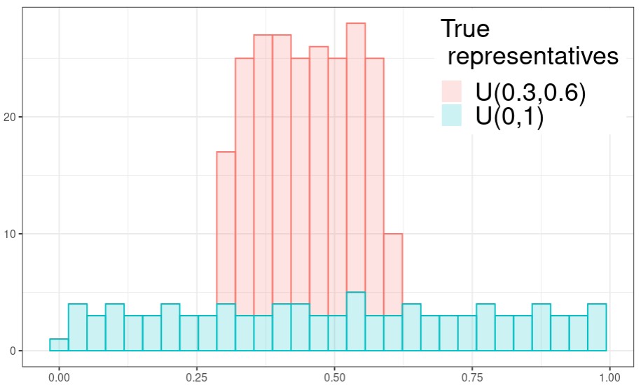
Figure 1: Distribution of $S_{u}$.

The quantization algorithms start from the two representatives $R_{1}=R_{U}(0,0.5)$ and $R_{2}=R_{U}(0.5,1)$. Regarding the $FindR$ step, that provides representatives from clusters, we investigate for each cluster $C_{j}$ and for each dimension $k=1,\dots,m$, ($m=1$ here) the best parameters $(a_{j}^{k},b_{j}^{k})\in\mathbb{R}^{2}$ minimizing $\mathcal{W}_{2}(C_{j}^{k},R_{U}(a_{j}^{k},b_{j}^{k}))$, where $C_{j}^{k}=\{x^{k}\,:\;(x^{1},\dots,x^{m})\in C_{j}\}$. Denoting $Q_{j}^{k}$ the empirical quantile function of $C_{j}^{k}$, the optimal uniform representative can be explicitly calculated as

$$\begin{multlined}\left\{\begin{array}[]{ll}a_{j}^{k}=\int_{0}^{1}Q_{j}^{k}(q)(-6q+4)dq\\ b_{j}^{k}=\int_{0}^{1}Q_{j}^{k}(q)(6q-2)dq\end{array}\right.\end{multlined}\left\{\begin{array}[]{ll}a_{j}^{k}=\int_{0}^{1}Q_{j}^{k}(q)(-6q+4)dq\\ b_{j}^{k}=\int_{0}^{1}Q_{j}^{k}(q)(6q-2)dq\end{array}\right.$$

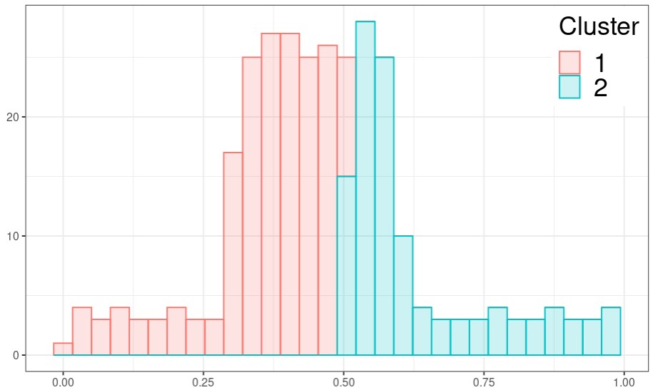
Figure 2: Distribution of two clusters provided by the $FindC$ step started from the representatives $R_{1}=R_{U}(0,0.5)$ and $R_{2}=R_{U}(0.5,1)$.

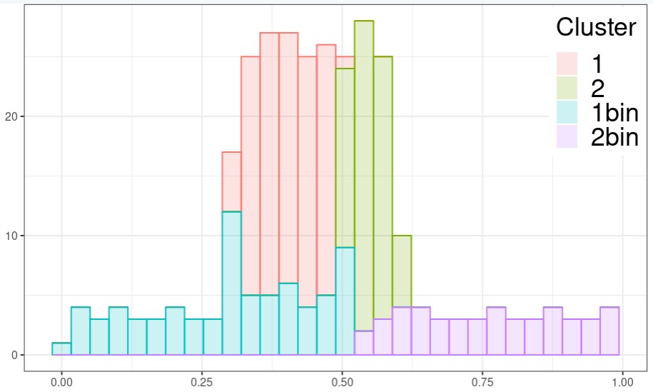
(a)

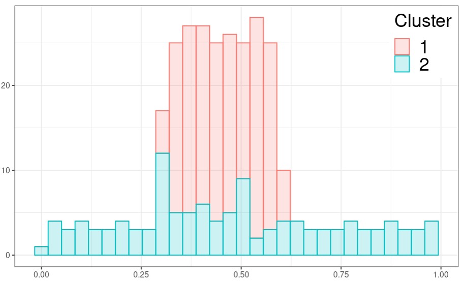
(b)

Figure 3: $Perturb$ step with $p_{\mathrm{bin}}=0.4$. Figure 3(a) shows the $split$ into 4 clusters, and Figure 3(b) is the result of the $merge$ phase: clusters 1 and 2 are grouped, clusters 1bin and 2bin are grouped too. Clusters 1bin and 2bin are the elements removed from clusters 1 and 2, respectively.

The first $FindC$ step of Algorithm 2 yields the two clusters shown in Figure 2. The $Perturb$ step is illustrated in Figure 3 with $p_{\mathrm{bin}}=0.4$. Then the $FindR$ function provides two new representatives, $R_{1}=R_{U}(0.31,0.60)$ and $R_{2}=R_{U}(0.03,0.93)$. This single iteration is enough to get close to the representatives of the investigated mixture. At the completion of the other iterations, the estimated mixture $R_{J^{\star}}^{\star}$ reported in Table 1 is found. This mixture is represented in Figure 4(b), with the optimal clusters illustrated in Figure 4(a). The optimal quantization error is $\mathcal{E}_{2}(\bm{C}^{\star},\bm{R}^{\star})=4.4\times 10^{-3}$ and the global error is $\epsilon_{2}(\bm{C}^{\star},\bm{R}^{\star})=3.0\times 10^{-3}$. As shown in Table 1, this global error is slightly lower than that between the true mixture and the sample. Thus, the algorithm finds a solution whose accuracy is of the order of the sampling error.

To test the robustness of the method, the previous experiment is repeated with 15 other samples made of $300$ points obtained from Sobol sequences that represent mixtures of respective densities $f_{i}=p_{i}\frac{\mathds{1}_{[a_{i},b_{i}]}}{b_{i}-a_{i}}+(1-p_{i})\frac{\mathds{1}_{[c_{i},d_{i}]}}{d_{i}-c_{i}}$, with $a_{i},b_{i},c_{i},d_{i},p_{i}\in[0,1]$ sampled such that $b_{i}>a_{i}$ and $d_{i}>c_{i}$. The resulting distributions of the quantization errors and the global errors and the comparison with the errors of the true mixtures are shown in Figure 5. The errors are low throughout the repetitions. For example, the median quantization error, which falls below $2\times 10^{-3}$, is smaller than the one achieved with the true mixtures. The distribution of the global errors have a similar pattern. The evolution of the quantization error throughout the iterations is described in Appendix G.

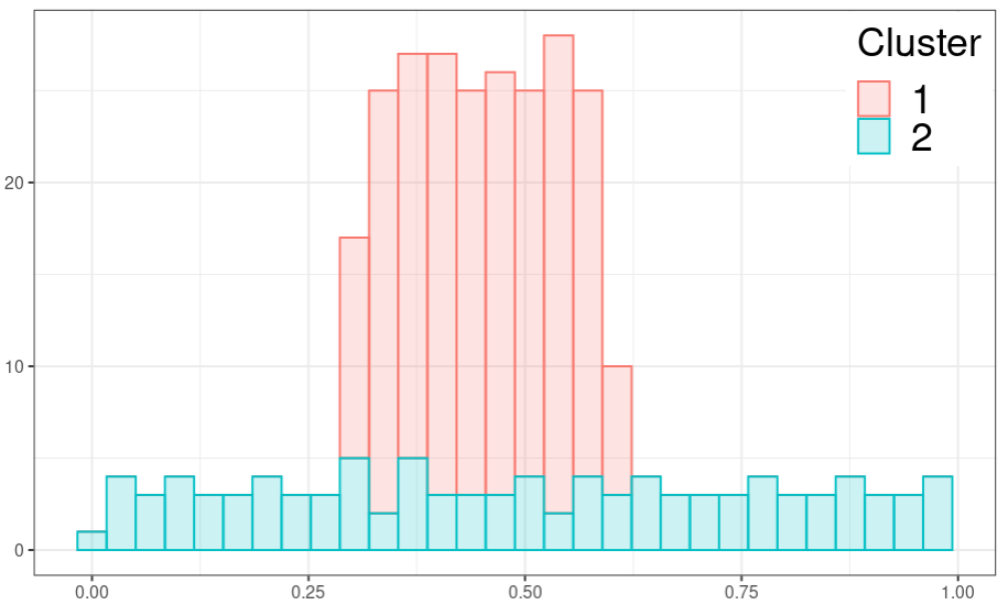
(a)

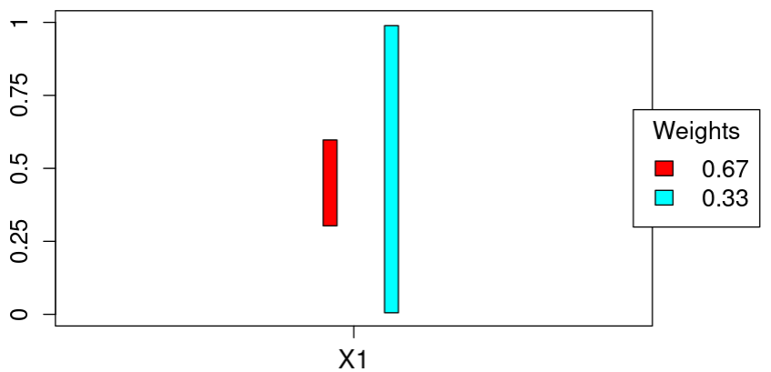
(b)

Figure 4: 4(a): The optimal clusters estimated by AQ. 4(b): The optimal representatives and their weights. Each color is associated to a representative, and the support of the uniform distributions are plotted as a vertical bar.

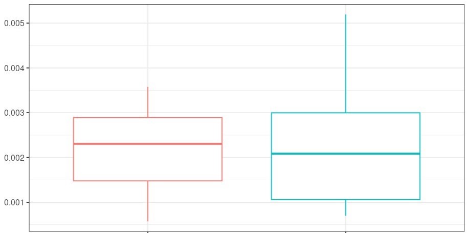
(a) Quantization error distribution of the true mixtures (red) and of the mixtures estimated by AQ (blue).

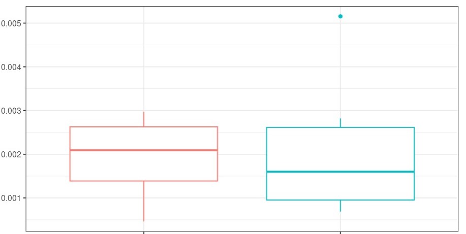
(b) Global error distribution of the true mixtures (red) and of the mixtures estimated by AQ (blue).

Figure 5: Distributions of the errors in the uniform test case.

5.2 A mixture of Dirac example

We now assume that the representatives are delta Dirac measures, which corresponds to the classical quantization problem: we have $\mathcal{R}=\{\delta_{\gamma},\gamma\in\mathcal{X}\}$, where $\delta_{\gamma}$ is the Dirac measure at the point $\gamma$.

The $FindC$ procedure described in Section 4.1 is equivalent to the computation of the Voronoï cells in Lloyd’s algorithm. From $\bm{R}=(\delta_{\gamma_{1}},\dots,\delta_{\gamma_{\ell}})$, it provides $\bm{C}=(C_{1},\dots,C_{\ell})$ with $C_{j}=\{x\,:\;j=\underset{j^{\prime}}{\argmin}\lVert x-\gamma_{j^{\prime}}\lVert\}$.

The $FindR$ step of Section 4.3 amounts to finding, for all clusters $j$, $\gamma_{j}$ minimizing

$$\mathcal{W}_{2}(\gamma,C_{j})^{2}=\frac{1}{\mathrm{card}\left(C_{j}\right)}\sum_{x\in C_{j}}\lVert x-\gamma\lVert^{2}.$$

The solution is, for $j\in\mathcal{J}$,

$$\gamma_{j}=\frac{1}{\mathrm{card}\left(C_{j}\right)}\sum_{x\in C_{j}}x.$$

With Dirac representatives, like for $FindC$, $FindR$ degenerates into a step of Lloyd’s algorithm. Note that it is equivalent to optimize the sum of the Wasserstein distances on each marginal, as proposed in Section 4.3.

In the Dirac case, the Augmented Quantization is identical to the classical K-means quantization, but with an additional step of clusters perturbation. We now investigate the effect of this operation.

Lloyd’s algorithm and AQ are compared on $500$ different samples of 20 points with $20$ starting clusters centers tested for each sample,which means a total of $2\times 10^{4}$ runs. The samples are i.i.d. realizations of a uniform distribution in $[0,1]^{2}$, and the quantization is performed with two representatives. Figure 6 shows one example of the results. For each of these tests, the quantization errors (Equation (1)) are computed for the two methods, and are denoted $\mathcal{E}_{\mathrm{Lloyd}}$ and $\mathcal{E}_{\mathrm{AQ}}$ for Lloyd’s algorithm and AQ, respectively.

The distribution of the difference, $\frac{\mathcal{E}_{\mathrm{Lloyd}}-\mathcal{E}_{\mathrm{AQ}}}{\mathcal{E}_{\mathrm{Lloyd}}}\times 100$, is provided in Figure 7. In $44\%$ of the tests, both methods have the same quantization error. AQ outperforms Lloyd’s algorithm (as characterized by a negative relative difference) in $50\%$ of the cases.

The median of the improvement of AQ over Lloyd is $3.1\%$, and the third quartile is $7.7\%$. Thanks to the cluster perturbation, the Augmented Quantization produces significantly better results than K-means in the Dirac case.

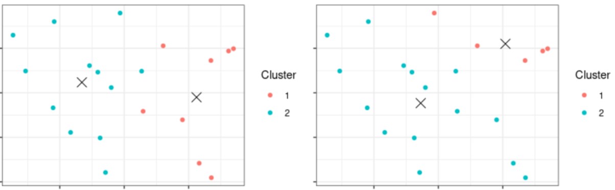
Figure 6: An example of the optimal clusters (red and blue dots) and their centroids (black crosses) obtained with Lloyd’s algorithm (left) and AQ (right). Both algorithms were started with the same representatives (i.e., here, cluster centers). The quantization error is 0.28 with Lloyd’s algorithm and 0.25 with AQ.

Figure 7: Distribution of the relative difference (in $\%$) between the quantization errors of Lloyd’s algorithm and AQ. Negative values correspond to a better performance of AQ.

5.3 A Gaussian mixture example

The Gaussian mixture models, denoted GMM and estimated with the EM algorithm are very popular when it comes to identifying Gaussian representatives. In the following example, we compare the Augmented Quantization with this GMM in one dimension. The representatives belong to $\mathcal{R}=\{R_{N}(\mu,\sigma^{2}),(\mu,\sigma)\in\mathbb{R}^{2}\}$ where $R_{N}$ is the measure associated to $\mathcal{N}(\mu,\sigma^{2})$.

The $FindR$ step is the minimization of $\mathcal{W}_{2}(C_{j}^{k},R_{N}(\mu_{j}^{k},(\sigma_{j}^{k})))$, for each cluster $C_{j}$ and each dimension $k=1,\dots,m$, ($m=1$ here). It leads to

$$\left\{\begin{array}[]{ll}\mu_{j}^{k}&=\int_{0}^{1}Q_{j}^{k}(q)dq=\frac{1}{\mathrm{card}\left(C_{j}^{k}\right)}\sum_{x\in C_{j}^{k}}x\\ \sigma_{j}^{k}&=\frac{\int_{0}^{1}Q_{j}^{k}(q)\mathrm{erf}^{-1}(2q-1)dq}{\sqrt{2}\int_{0}^{1}\left(\mathrm{erf}^{-1}(2q-1)\right)^{2}dq}\end{array}\right.$$

where $\mathrm{erf}$ is the error function defined by $\mathrm{erf}(z)=\frac{2}{\sqrt{(}\pi)}\int_{0}^{z}\exp{(-t^{2})}dt$.

It is important to note that this $FindR$ procedure leads to representatives with independent marginals, while GMM can describe a covariance structure.

We consider a family of samples $(S_{g}^{i})_{i=1}^{15}$, made of $400$ points obtained with Gaussian transformations of Sobol sequences. They represent mixtures of density $f_{i}(x)=p_{i}\frac{1}{\sigma_{i}^{1}\sqrt{2\pi}}exp(-(\frac{x-\mu^{1}_{i}}{\sigma^{1}_{i}})^{2})+(1-p_{i})\frac{1}{\sigma_{i}^{2}\sqrt{2\pi}}exp(-(\frac{x-\mu^{2}_{i}}{\sigma^{2}_{i}})^{2})$, with $\mu^{1}_{i}$, $\sigma^{1}_{i}$, $\mu^{2}_{i}$, $\sigma^{2}_{i}$, $p_{i}$ randomly sampled in $[0,1]$.

The distributions of the quantization and global errors are provided in Figure 8. The quantization error cannot be computed for GMM because the elements of the sample are not assigned to a cluster but belong to clusters in probability. On the opposite, the global error (formula (4)) of GMM can be calculated. The median of the distribution of AQ’s quantization errors is very close to that of the true mixtures with a lower dispersion. The distributions of AQ and the true global errors compare identically: the median of the true mixture is sligthly lower but its spread slightly higher. This also shows that the AQ error is much lower than the sampling error. The GMM scheme, on the other hand, identifies with slightly better global errors. Note that these errors are one order of magnitude higher than those observed in the uniform test case. Indeed, the samples obtained by quasi-Monte Carlo methods are closer to their targeted distribution in the uniform case than in the Gaussian one.

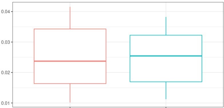
(a) Distribution of the quantization errors for the true mixtures (red) and the mixtures obtained through AQ (blue).

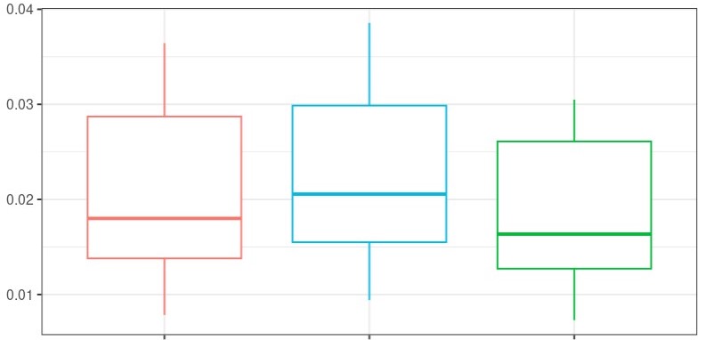
(b) Distribution of the global errors for the true mixtures (red), the mixtures obtained through AQ (blue), and the GMM approach (green).

Figure 8: Distributions of the errors in the Gaussian test case.

Figure 9(a) displays the distribution of the sample $S_{g}^{t}$ that corresponds to the median global error obtained with AQ. $S_{g}^{t}$ is chosen as a typical sample of the Gaussian test case. Table 2 summarizes, for this median sample $S_{g}^{t}$, the mixtures identified by the various methods along with their global errors. Even though GMM finds a closer to the sample than AQ does, Figure 9(c) illustrates that both distributions are close to each other. Figure 9(b) further shows that the clusters identified by AQ closely match the distributions of their representatives.

To conclude about the experiments made on the Gaussian test case, both GMM and AQ identify relevant sub-distributions, but GMM which is specifically designed to handle Gaussian mixtures remains slightly better. Of course, GMM is less general than AQ as it cannot mix distributions of different types such as Gaussian, uniform or Dirac measures.

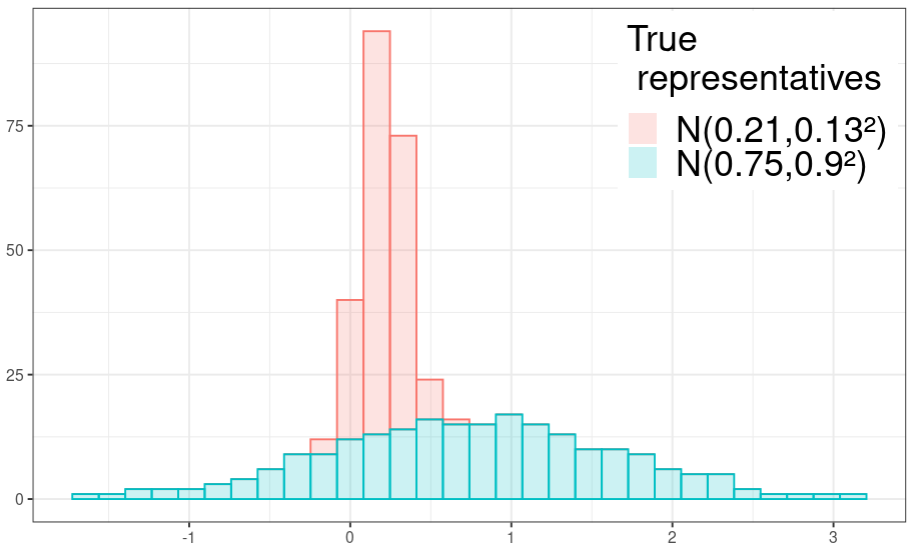
(a) Distribution of $S_{g}^{t}$

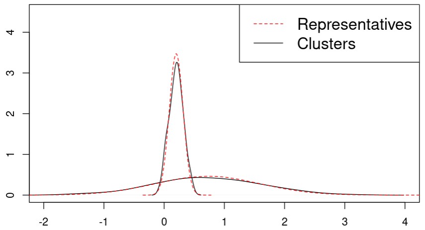
(b) Density of the optimal clusters and their representatives estimated with AQ for the sample $S_{g}^{t}$.

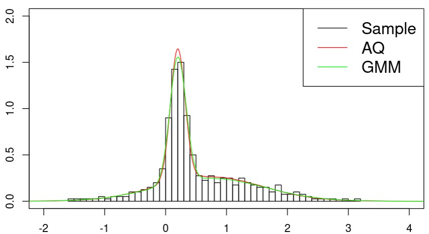
(c) Illustration of the mixtures identified by AQ and GMM on the typical sample $S_{g}^{t}$. Gaussian test case.

Figure 9: Illustration of AQ and GMM with the sample $S_{g}^{t}$.

True mixture	AQ mixture	GMM Mixture
$R_{1}^{\mathrm{true}}=R_{N}(0.21,0.13^{2})$	$R_{1}^{\star}=R_{N}(0.20,0.12^{2})$	$R_{1}^{\mathrm{GMM}}=R_{N}(0.20,0.13^{2})$
$R_{2}^{\mathrm{true}}=R_{N}(0.75,0.9^{2})$	$R_{2}^{\star}=R_{N}(0.72,0.86^{2})$	$R_{2}^{\mathrm{GMM}}=R_{N}(0.74,0.89^{2})$
$\mathbb{P}(J_{\mathrm{true}}=1)=0.45$	$\mathbb{P}(J^{\star}=1)=0.4$	$\mathbb{P}(J_{\mathrm{GMM}}=1)=0.38$
$\mathbb{P}(J_{\mathrm{true}}=2)=0.55$	$\mathbb{P}(J^{\star}=2)=0.6$	$\mathbb{P}(J_{\mathrm{GMM}}=2)=0.62$
$W_{2}(S^{t}_{g},R_{J_{\mathrm{true}}}^{\mathrm{true}})=2.9\times 10^{-3}$	$W_{2}(S^{t}_{g},R_{J^{\star}}^{\star})=3.3\times 10^{-2}$	$W_{2}(S^{t}_{g},R_{J_{\mathrm{GMM}}}^{\mathrm{GMM}}))=2.9\times 10^{-3}$

Table 2: True and estimated mixture with AQ and with GMM in the Gaussian test case $S_{g}^{t}$ in 1D. $W_{2}(S^{t}_{g},R_{J_{\mathrm{true}}}^{\mathrm{true}})$, $W_{2}(S^{t}_{g},R_{J^{\star}}^{\star})$, and $W_{2}(S^{t}_{g},R_{J_{\mathrm{GMM}}}^{\mathrm{GMM}}))$ are the global errors between the clusterings and the mixtures.

6 An hydrib mixture test case

To illustrate the possibilities of augmented quantization compared to existing schemes such as GMM, we now cover the case of a hybrid mixture made of a Gaussian and a uniform representative.

We consider a sample $S_{\mathrm{hyb}}$ of 350 points distributed to represent a mixture of density $f_{\mathrm{hyb}}=\frac{1}{3}\mathds{1}_{[0.2,0.5]}+\frac{2}{3}\frac{1}{0.2\sqrt{2\pi}}exp(-(\frac{x-0.6}{0.2})^{2})$. The sample is displayed in Figure 10(a). The results of AQ are shown in Figure 10(b). The two representatives are well identified by AQ, leading to a quantization error of $8.3\times 10^{-3}$ and a global error equal to $7.6\times 10^{-3}$.

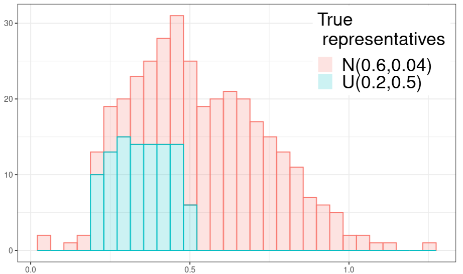
(a) Distribution of $S_{\mathrm{hyb}}$.

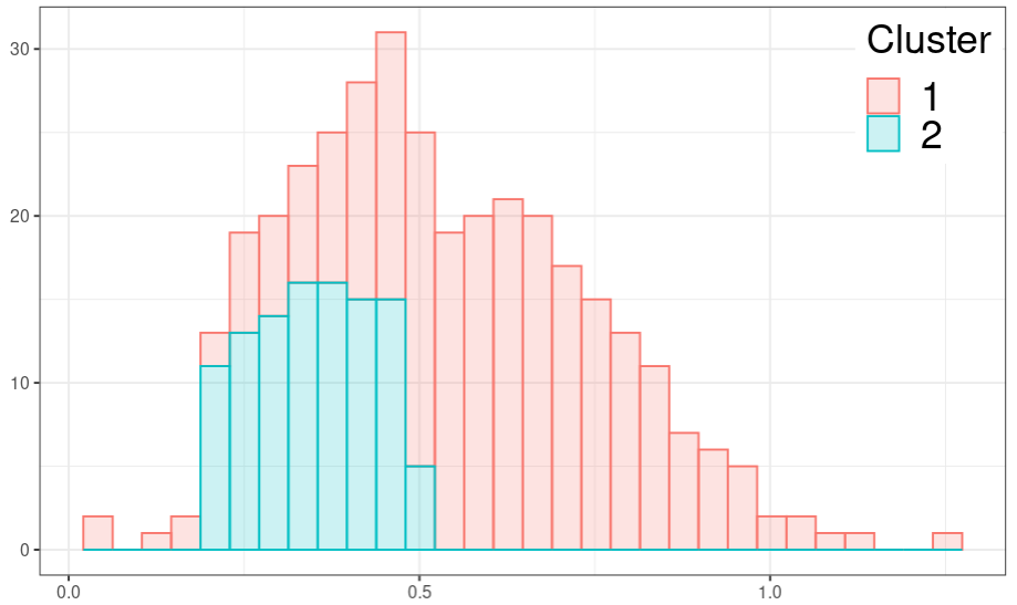
(b) Clusters estimated by AQ from the sample $S_{\mathrm{hyb}}$.

Figure 10: Hybrid case of a Gaussian and a uniform mixture. Data (left) and distribution of the clusters identified by AQ (right).

To investigate the robustness of AQ, a family of samples $(S_{\mathrm{hyb}}^{i})_{i=1}^{15}$ of size $350$ is considered. A comparison between the true mixtures and the mixtures estimated by AQ is provided in Figure 11. These boxplots illustrate that the identified mixtures represent well the samples, with distributions of errors near the distributions of the errors obtained with the true mixtures. The additional error of AQ is very small compared to the sampling error. It is attributed to limited size of the samples.

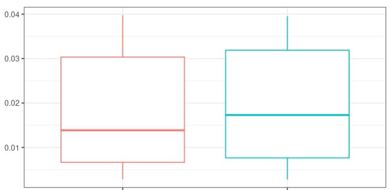
(a) Distribution of the quantization errors for the true mixtures (red) and the mixtures estimated by AQ (blue).

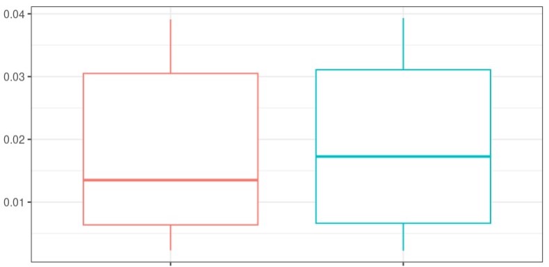
(b) Distribution of the global errors for the true mixtures (red) and the mixtures estimated by AQ (blue).

Figure 11: Distributions of the errors in the hybrid test case.

7 Application to river flooding

Thanks to its ability to mix uniform and Dirac measures, Augmented Quantization can be applied to the sensitivity analysis of numerical simulators of a real systems. The broad-based goal of a sensitivity analysis is to assess the impact of an uncertainty of the inputs on the uncertainty of the output. A review of the recent advances can be found in [5].

Our proposal for an AQ-based sensitivity analysis starts by estimating a mixture to represent the distribution of the inputs that lead to a specific output regime. The idea is to bring information about the causes of this regime. We compare the overall input distribution to their conditional distribution given the output belongs to the investigated output regime. Similar approaches have already been conducted with Hilbert-Schmidt Independence Criterion in [spagnol]. If an input variable has the same marginal distribution in the identified mixture as in the original distribution, then this variable has no direct influence on the triggering of the output regime. Vice versa, if the support of the marginal distribution of an input of the identified mixture is narrower than its original support, then its value contributes to the phenomenon under scrutiny. Although the sensitivity analysis of groups of variables could follow the same principle, it would require extensions that are out of the scope of this paper.

As a specific example, we investigate the probabilistic distribution of flood maps. The inputs are features of the environment that are possible causes of the floodings. The case study focuses on a section of the Loire River near Orléans, France, which is flanked by levees on both banks and has a history of significant flooding in the 19th century. The area studied, including historical levee breaches ([12]) is illustrated in Figure 12.

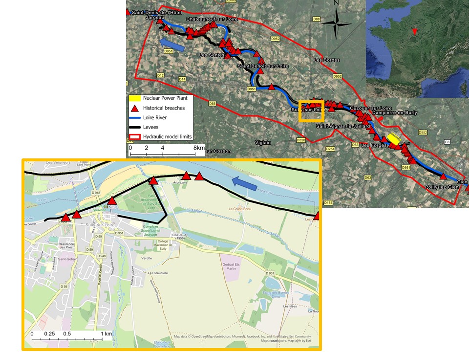
Figure 12: Study area of the flooding test case, including the levees and the historical breaches ([16]). The zones of the roughness coefficients ($K_{\mathrm{s}3}$ and $K_{\mathrm{s}4}$) are delimited with the green lines.

To simulate the river flow of the Loire River between Gien and Jargeau over a distance of 50 km, the Institute for Radiological Protection and Nuclear Safety (IRSN) has built a hydraulic model using the open-source TELEMAC-2D simulator ([19]). The model incorporates an upstream hydrograph and a calibration curve as boundary conditions and has been calibrated using well-known flood events by adjusting the roughness coefficients (Strickler coefficients). Breaches are considered as well, leading to the study of four variables, considered as independent:

• The maximum flow rate ($Q_{\mathrm{max}}$) which follows a Generalized Extreme Value distribution, established using the Loire daily flow rate at Gien.

• Two roughness coefficients ($K_{\mathrm{s}3}$ and $K_{\mathrm{s}4}$) of specific zones illustrated in Figure 12 that are calibration parameters. These coefficients are calculation artifacts and are not observed in real-world data sets. Therefore, triangular distributions are employed and the mode of these distributions corresponds to the calibration values defined for each roughness area.

• The erosion rate ($er$), describing the vertical extent of the breach during the simulated time, which follows a uniform distribution.

Due to the large size of the area that is modeled, our focus is limited to the left bank sector of the river, specifically Sully-sur-Loire. There, we have simulated seven breaches whose sites and lengths correspond to those of the actual history.

Through quantization, we want to perform a sensitivity analysis of the inputs leading to the most severe floodings.

As a preliminary step, a classical quantization is performed in the output space of floodings maps (expressed as water heights outside of the river domain) with the approach detailed in [24]. 1000 flooding maps are simulated with the hydraulic model and form a training dataset to build the metamodel. This metamodel is generative in the sense that it is based on Gaussian processes. $10^{6}$ maps are then sampled from the metamodel and quantized with a mixture of 5 Dirac distributions thanks to the R package FunQuant ([23]). This yields the 5 prototype maps, 5 clusters of floodings and the corresponding probabilities provided in Appendix H.

We specifically focus on analyzing the input distribution associated with the most severe pattern, which has a probability of $5.8\times 10^{-4}$. The inputs are mapped through the empirical cumulated distribution function of each marginal for all the floodings, which amounts to use the rank statistics of the inputs instead of their actual values. It is indeed well-known that the distribution of these normalized inputs is uniform on each marginal. This transformation facilitates the comparison of the overall input distribution, which is thus uniform on the whole support by definition, with that of the inputs leading to a specific regime.

To accomplish this, Augmented Quantization is executed within the cluster of most severe floodings with a sample of 500 elements: maps are generated with the metamodel following the overall distribution of the inputs until 500 maps are associated to the investigated regime.

The identified mixtures contain 3 representatives that can be a Dirac or uniform distributions with a support of width $0.25$, $0.5$ or $1$. This allows to highlight influential variables: the distribution of a variable that has no impact on the extreme floodings should remain a uniform between 0 and 1 while values concentrated around specific values reveal a directly explanatory variable. The family of measures considered here is written $\mathcal{R}=\{R(\alpha_{1},\dots,\alpha_{4},a_{1},\dots,a_{4},\sigma_{1},\dots,\sigma_{4})\}$ where $R=R_{1}\times\dots\times R_{4}$ with

$$\begin{multlined}R_{i}([x_{1},x_{2}])=\\ \biggl{[}\alpha_{i}\frac{min(x_{2},a_{i}+\frac{\sigma_{i}}{2})-max(x_{1},a_{i}-\frac{\sigma_{i}}{2})}{\sigma_{i}}\\ +(1-\alpha_{i})\mathds{1}_{[x_{1},x_{2}]}(a_{i})\biggr{]}\mathds{1}_{[a_{i}-\frac{\sigma_{i}}{2},+\infty[}(x_{2})\end{multlined}R_{i}([x_{1},x_{2}])=\\ \biggl{[}\alpha_{i}\frac{min(x_{2},a_{i}+\frac{\sigma_{i}}{2})-max(x_{1},a_{i}-\frac{\sigma_{i}}{2})}{\sigma_{i}}\\ +(1-\alpha_{i})\mathds{1}_{[x_{1},x_{2}]}(a_{i})\biggr{]}\mathds{1}_{[a_{i}-\frac{\sigma_{i}}{2},+\infty[}(x_{2})$$

with $(\alpha_{1},\dots,\alpha_{4},a_{1},\dots,a_{4},\sigma_{1},\dots,\sigma_{4})\in\{0,1\}^{4}\times[0,1]^{4}\times\{0.25,0.5,1\}.$

Figure 13 presents the representatives estimated with AQ to approximate the distribution of inputs leading to the most severe floodings. Each of the 3 representatives is associated to a color (blue, green and red). A vertical bar materializes the support of a uniform distribution. A triangle indicates the position of a Dirac. This study shows the major influence of the maximum flow rate, $Q_{\mathrm{max}}$, as only Dirac distributions are identified at ranks very close to 1, meaning that only very high values of $Q_{\mathrm{max}}$ yield these extreme events.

The impact of the roughness in the zone associated with $K_{\mathrm{s}4}$ is also evident. Lower values of $K_{\mathrm{s}4}$ appear to promote intense floodings, as evidenced by the main blue representative of probability $60\%$ that exhibits a uniform distribution of width $0.25$ between $K_{\mathrm{s}4}=0$ and $K_{\mathrm{s}4}=0.25$. On the other hand, the influence of the low values of the roughness in the zone of $K_{\mathrm{s}3}$ is relatively weaker, its main representative (in blue) being a uniform between $0$ and $1$. However, it has a joint influence with $K_{\mathrm{s}4}$, as observed in the blue and green representatives. This combination accounts for a combined probability mass of approximately $87\%$, where either $K_{\mathrm{s}3}$ or $K_{\mathrm{s}4}$ is lower than 0.5. These results can be interpreted by remembering that $K_{\mathrm{s}4}$ is a roughness in a section of the river downstream of the section of $K_{\mathrm{s}3}$.

Interestingly, the high erosion rates, $er$, that describe important breaches, do not seem to have a significant impact on the most severe flooding events: only $13\%$ of the probability mass is represented by a small uniform, the red representative that has a support between $0.42$ and $0.92$. The rest of the mass is a uniform between $0$ and $1$. This can be attributed to the extremely high flow rates $Q_{\mathrm{max}}$ involved, which render the breach impact almost negligible since water flows over the levees anyway.

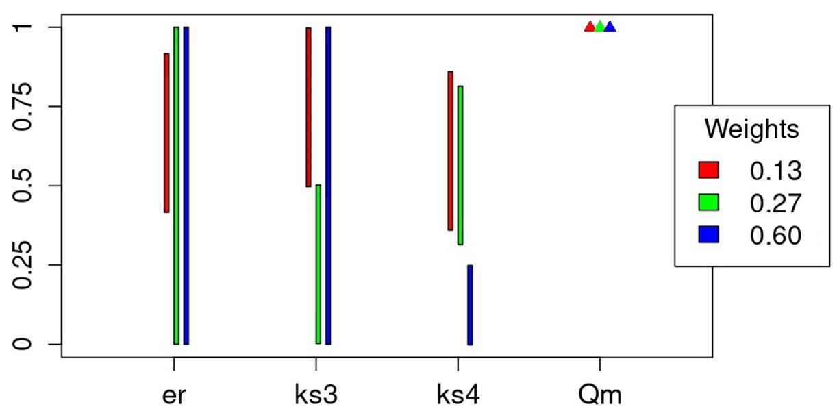
Figure 13: Mixture of Dirac and uniform distributions estimated by AQ and approximating the distribution of the parameters associated to the most severe floodings. Each color corresponds to one of the three representatives. A vertical bar is a uniform distribution, and a triangle indicates the position of a Dirac.

8 Summary and perspectives

This work proposes an Augmented Quantization (AQ) scheme to build mixture models from a sample $(x_{i})_{i=1}^{n}$. It extends the classical Lloyd’s algorithm which generates Dirac mixtures by minimizing the quantization error of Equation (1) through repeated clustering and centroid calculations. The quantization error can be reformulated with the Wasserstein distance to extend it to all types of distributions, discrete or continuous, with finite or infinite support. AQ is then more general than the classical mixture modeling approaches based on the Expectation-Maximization algorithm. AQ minimizes a Wasserstein-based quantization error over a space of probability measures called representatives. AQ proceeds by repeating clustering, clustering perturbation and representatives estimation calculations. The decomposition of the quantization error minimization into clustering and representatives estimation reduces the numerical complexity of the method compared to a direct optimization of the mixture parameters. For example, the number of parameters to optimize three uniform representatives in 3D is 20 but it reduces to 6 parameters by clusters. With respect to K-means algorithms, the cluster perturbation is also new. It is added to make the approach more robust to the initial choice of representatives.

We have provided some theoretical guarantees about AQ. The cluster perturbation and the representatives estimation locally minimize the quantization errors. The clustering scheme is asymptotically consistent with respect to the current mixture.

Tests with homogeneous mixtures of Dirac, uniform and Gaussian unidimensional distributions have been performed. They are completed by a four-dimensional application to river floodings where Dirac and uniform representatives are mixed. The results of these tests are promising, yet several areas of improvement are worth exploring.

Tuning of the cluster perturbation intensity.

In our implementation of AQ, the cluster perturbation intensity is tuned through the parameters $\ell_{\mathrm{bin}}$ and $p_{\mathrm{bin}}$. While $\ell_{\mathrm{bin}}$, the number of clusters to split, is fixed by the numerical complexity of the algorithm, $p_{\mathrm{bin}}$, the proportion of points to remove from clusters that are split, was tuned manually.

An improved version of the method could adapt online the proportion $p_{\mathrm{bin}}$. An ingredient towards such adaptation is to detect a cut-off point in clustering error after splitting.

Active learning of the number of representatives.

The AQ method described here maintains a constant number of clusters (i.e., representatives). This number is chosen a priori, which assumes some knowledge of the data structure. In a more general scenario, cluster perturbation could modify the number of clusters based on the Wasserstein distances between the clusters (including the bins) and their representatives. For example, some merges could significantly increase the quantization error, indicating that the number of clusters should increase. While such ideas should be explored, they are likely to add computational complexity to the method.

Computational cost.

The computational cost of the current AQ algorithm restricts the sample size to be less than several thousands because of the execution of greedy algorithms. The split operation has the largest complexity, as the selection of the point to transfer from the cluster to the bin necessitates computing Wasserstein distances for all possible transfers. To alleviate the computational burden, it may be worthwhile to investigate batch and incomplete transfer approaches, although this may reduce precision. As the overall complexity depends on the complexity of the Wasserstein distance, it may be opportune to approximate it by sliced Wasserstein distance ([15]).

Statements and Declarations

The authors declare that they have no known competing financial interests or personal relationships that could have appeared to influence the work reported in this paper.

SUPPLEMENTARY MATERIAL

Codes related to the uniform, dirac and gaussian test cases: Git repository containing R notebooks to reproduce all the experiments related to the test cases that are described in the article. (https://github.com/charliesire/augmented_quantization.git)

spagnol

Appendix A Expectation-Maximization with uniform mixtures

The combination of finite support measures with the use of likelihood loss function causes issues when learning mixtures. As an example, we detail the case of a mixture of uniform distributions.

Let us consider $(X^{1},\dots,X^{n})$ i.i.d. random variables, and a realization $S_{\mathrm{EM}}=(x_{i})_{i}^{n}$. We approximate the distribution by a mixture with two representatives $U(a_{1},b_{1})$ and $U(a_{2},b_{2})$. The bounds and the weights $p_{1}$ and $p_{2}=1-p_{1}$ of the representatives are calculated by maximum likelihood as in the Expectation maximization algorithm. Let us denote $\theta=(a_{1},b_{1},a_{2},b_{2},p_{1})$. The likelihood function is

$$\mathcal{L}(\theta)=\prod_{i=1}^{n}\left(p_{1}\frac{\mathds{1}_{[a_{1},b_{1}]}(x_{i})}{b_{1}-a_{1}}+(1-p_{1})\frac{\mathds{1}_{[a_{2},b_{2}]}(x_{i})}{b_{2}-a_{2}}\right)\leavevmode\nobreak\ .$$

The EM algorithm starts with an initial set of parameters $\theta^{(0)}$, and aims at converging to an optimal $\theta^{\star}$ by maximizing the likelihood. EM introduces a latent random variable $Z=(Z_{1},\dots,Z_{n})$ indicating to which representative the elements are assigned.

The E-step performs a soft-assignment, attributing to each sample element a probability of being associated to each representative $j$ ([14]):

$$\forall i=1,\ldots,n\leavevmode\nobreak\ ,$$

$$\mathbb{P}(Z_{i}=j\mid\theta) =p_{Z_{i}\mid x_{i}}(j\mid x_{i};\theta)$$

$$=\frac{p_{x_{i}\mid Z_{i}}(x_{i}\mid Z_{i}=j;\theta)p_{j}}{P_{x_{i}}(x_{i}\mid\theta)}.$$

The M-step estimates the new parameters $\theta^{\mathrm{new}}$ by maximizing the marginal likelihood ([25]):

$$\theta^{\mathrm{new}}=\underset{\theta}{\argmax}\>\mathbb{E}_{Z}\left(p_{X\mid Z}(x\mid Z,\theta)p_{Z}(Z)\right).$$

We now run an iteration of the EM algorithm and analyze how it works with uniform mixtures.

The initial parameters are $a_{1}=\min x_{i}$, $b_{1}=0.5$, $a_{2}=0.5$, $b_{2}=\max(x_{i})_{i}^{n}$, and $p_{1}=p_{2}=0.5$.

The E-step assigns a probability to each pair of element and representative.

For $i=1:n$ and $j=1:2$,

$$\mathbb{P}(Z_{i}=j\mid\theta)=\frac{\frac{1}{2}\frac{\mathds{1}_{[a_{j},b_{j}]}(x_{i})}{b_{j}-a_{j}}}{\frac{1}{2}\frac{\mathds{1}_{[a_{1},b_{1}]}(x_{i})}{b_{1}-a_{1}}+\frac{1}{2}\frac{\mathds{1}_{[a_{2},b_{2}]}(x_{i})}{b_{2}-a_{2}}}$$

. Thus, if $x_{i}<0.5$, $\mathbb{P}(Z_{i}=1)=1$ and $\mathbb{P}(Z_{i}=2)=0$. If $x_{i}>0.5$, $\mathbb{P}(Z_{i}=1)=0$ and $\mathbb{P}(Z_{i}=2)=1$. The M-step aims at determining parameters $\theta^{\mathrm{new}}=(a^{\mathrm{new}}_{1},b^{\mathrm{new}}_{1},a^{\mathrm{new}}_{2},b^{\mathrm{new}}_{2},p^{\mathrm{new}}_{1})$ maximizing $\mathbb{E}_{Z}\left(p_{X\mid Z}(x\mid Z,\theta)p_{Z}(Z)\right)=\displaystyle\prod_{i,x_{i}<0.5}p_{1}\frac{\mathds{1}_{[a_{1},b_{1}]}(x_{i})}{b_{1}-a_{1}}\displaystyle\prod_{i,x_{i}>0.5}(1-p_{1})\frac{\mathds{1}_{[a_{2},b_{2}]}(x_{i})}{b_{2}-a_{2}}$. The optimization leads to $a_{1}=\min x_{i}$, $b_{1}=\underset{i,x_{i}<0.5}{\max}x_{i}$, $a_{2}=\underset{i,x_{i}>0.5}{\min}x_{i}$, $b_{2}=\max x_{i}$.

Now, let us suppose that the sample $S_{\mathrm{EM}}$ is the one illustrated in Figure 14, but without the points below 0 so that its distribution is almost a mixture of two representatives $\mathcal{U}(0,1)$ and $\mathcal{U}(0.7,0.9)$.

It appears that the clusters created by the above EM will not evolve through the iterations and the algorithm will not find such optimal representatives.

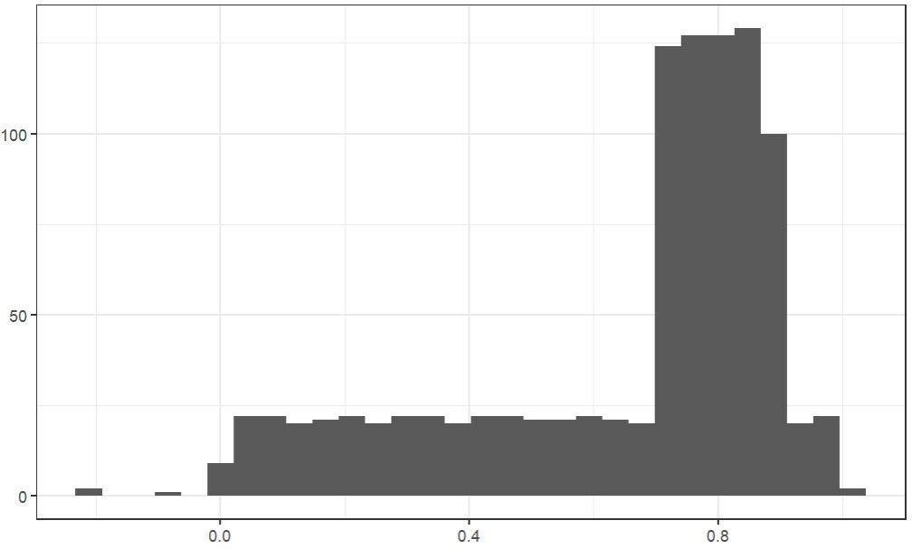
Figure 14: Distribution of the sample $S_{\mathrm{EM}}$.

Appendix B Augmented Quantization without perturbation

Here we perform AQ without the clusters perturbation, with the toy problem described in Section 5.1, starting from two representatives $R_{1}=R_{U}(0,0.5)$ and $R_{2}=R_{U}(0.5,1)$.

Figure 15 shows the clusters obtained after each of the first 9 iterations. The algorithm is rapidly stuck in a configuration far from the optimal quantization, with representatives around $R_{U}(0.26,0.93)$ and $R_{U}(0.19,0.63)$.

The obtained quantization error here is $4.0\times 10^{-2}$, more than $10$ times higher than the optimal quantization error obtained with Augmented Quantization including clusters perturbation, equal to $4.4\times 10^{-3}$ (see Section 5.1).

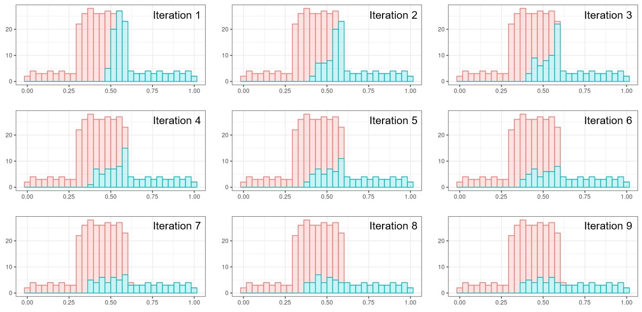
Figure 15: Distribution of clusters 1 and 2 in the 1D uniform case when performing the method without the clusters perturbation.

Appendix C Proof of Proposition 1

Let $\bm{R}=(R_{1},\dots,R_{\ell})$ be $\ell$ probability measures and $\bm{C}=(C_{1},\dots,C_{\ell})$ be $\ell$ disjoint clusters of points $\in\mathcal{X}\subset\mathbb{R}^{d}$. In addition, let us denote

• $n_{j}=\mathrm{card}\left(C_{j}\right)$ for $j\in\mathcal{J}$, and $n=\sum_{j=1}^{\ell}n_{j}$

• $\mu_{C}^{j}$ the empirical measure associated to $C_{j}$

• $\bm{\Pi}_{j}$ as the set of all coupling probabilities $\pi_{j}$ on $\mathcal{X}\times\mathcal{X}$ such that $\int_{\mathcal{X}}\pi_{j}(x,x^{\prime})dx=R_{j}(x^{\prime})$ and $\int_{\mathcal{X}}\pi_{j}(x,x^{\prime})dx^{\prime}=\mu_{C}^{j}(x)$

• $\pi^{\star}_{j}=\underset{\pi_{j}\in\bm{\Pi}_{j}}{\mathrm{inf}}\int_{\mathcal{X}\times\mathcal{X}}\lVert x-x^{\prime}\lVert^{p}\pi_{j}(x,x^{\prime})$

• $p_{j}=\frac{n_{j}}{n}$

• $\mu_{UC}$ the empirical measure associated to $\bigcup_{j=1}^{\ell}C_{j}$

• $\bm{\Pi}_{\mathrm{global}}$ as the set of all coupling probabilities $\pi$ on $\mathcal{X}\times\mathcal{X}$ such that $\int_{\mathcal{X}}\pi(x,x^{\prime})dx=R_{J}(x^{\prime})$ and $\int_{\mathcal{X}}\bm{\Pi}_{j}(x,x^{\prime})dx^{\prime}=\mu_{UC}(x)$

By definition of $R_{J}$, we have $R_{J}=\sum_{k=1}^{\ell}p_{j}R_{j}$. Similarly, we have $\mu_{UC}=\sum_{k=1}^{\ell}p_{j}\mu_{C}^{j}$.

$$\mathcal{E}_{p}(\bm{C},\bm{R}) =\left(\sum_{j}^{\ell}\frac{n_{j}}{n}\mathcal{W}_{p}(C_{j},R_{j})^{p}\right)^{\frac{1}{/}{p}}$$

$$=\left(\sum_{j=1}^{\ell}\frac{n_{j}}{n}\int_{\mathcal{X}\times\mathcal{X}}\lVert x-x^{\prime}\lVert^{p}\pi^{\star}_{j}(dx,dx^{\prime})\right)^{\frac{1}{p}}$$

$$=\left(\int_{\mathcal{X}\times\mathcal{X}}\lVert x-x^{\prime}\lVert^{p}\sum_{j=1}^{\ell}p_{j}\pi_{j}^{\star}(dx,dx^{\prime})\right)^{\frac{1}{p}}$$

$$=\left(\int_{\mathcal{X}\times\mathcal{X}}\lVert x-x^{\prime}\lVert^{p}\tilde{\pi}(dx,dx^{\prime})\right)^{\frac{1}{p}}$$

with $\tilde{\pi}=\sum_{j=1}^{\ell}p_{j}\pi_{j}^{\star}$.

Since for $j\in\mathcal{J},\pi_{j}^{\star}\in\bm{\Pi}_{j}$,

$$\int_{\mathcal{X}}\tilde{\pi}(dx,x^{\prime}) =\sum_{j=1}^{\ell}p_{j}\int_{\mathcal{X}}\pi_{j}^{\star}(dx,x^{\prime})$$

$$=\sum_{j=1}^{\ell}p_{j}R_{j}(x^{\prime})dx$$

$$=R_{J}(x^{\prime})\leavevmode\nobreak\ .$$

Similarly, $\int_{\mathcal{X}}\tilde{\pi}(x,x^{\prime})dx^{\prime}=\mu_{UC}(x)$. This shows that $\tilde{\pi}\in\bm{\Pi}_{\mathrm{global}}$.

Finally,

$$\epsilon_{p}(\bm{C},\bm{R}) =\mathcal{W}_{p}(\bigcup_{j=1}^{\ell}C_{j},R_{J})$$

$$=\underset{\pi\in\bm{\Pi}_{\mathrm{global}}}{\mathrm{inf}}\left(\int_{\mathcal{X}\times\mathcal{X}}\lVert x-x^{\prime}\lVert^{p}\pi(dx,dx^{\prime})\right)^{\frac{1}{p}}$$

$$\leq\mathcal{E}_{p}(\bm{C},\bm{R})\hskip 113.81102pt\square$$

Appendix D Proof of clustering consistency (Proposition 3)

We recall and complete our notations used to discuss clustering:

• The representative mixtures are $(R_{1},\dots,R_{\ell})\in\mathcal{R}_{s}^{\ell}$

• $J$ is a random variable with $\forall j\in\mathcal{J},\>P(J=j)=p_{j}$

• $(X_{k})_{k=1}^{n}$ are i.i.d. data samples and $X_{k}$ has probability measure $R_{J}$

• $(J_{i})_{i=1}^{N}$ are i.i.d. samples with same distribution as $J$

• $(Y_{i})_{i=1}^{N}$ are i.i.d. mixture samples and $Y_{i}$ has probability measure $R_{J_{i}}$

• The index of the representative whose sample is closest to $x$,$I_{N}(x)=\underset{i=1,\dots,N}{\argmin}{\lVert x-Y_{i}\rVert}$

• The mixture sample the closest to $x$, $a_{N}(x)=Y_{I_{N}(x)}\\ \mbox{{\color[rgb]{1,1,1}THE MIXTure sample the closest to ddddd}}=\arg\min_{y\in\{Y_{1},\ldots,Y_{N}\}}\lVert x-y\rVert$

• The $k$-th data sample that is assigned to cluster $j$, $\tilde{X}^{(j)}_{k,N}=X_{k}\mid J_{I_{N}(X_{k})}=j$. This of course does not mean that the $k$-th sample will belong to cluster $j$, which may or may not happen. It is a random vector whose probability to belong to cluster $j$ will be discussed.

The space of measures of the representatives is $\mathcal{R}_{s}:=\{\beta_{\mathrm{c}}R_{\mathrm{c}}+\beta_{\mathrm{disc}}R_{\mathrm{disc}},R_{\mathrm{c}}\in\mathcal{R}_{\mathrm{c}},R_{\mathrm{disc}}\in\mathcal{R}_{\mathrm{disc}},\beta_{\mathrm{c}}+\beta_{\mathrm{disc}}=1\}$ where

• $\mathcal{R}_{\mathrm{c}}$ is the set of the probability measures $R_{\mathrm{c}}$ for which the associated density (i.e. their Radon–Nikodým derivative with respect to the Lebesgue measure), exists, has finite support and is continuous almost everywhere in $\mathbb{R}^{d}$,

• $\mathcal{R}_{\mathrm{disc}}$ is the set of the probability measures of the form $R_{\mathrm{disc}}=\sum_{k=1}^{m}c_{k}\delta_{\gamma_{k}}$, with $\delta_{\gamma_{k}}$ the Dirac measure at $\gamma_{k}$ and $c_{k}\in[0,1]$ such that $\sum_{k=1}^{m}c_{k}=1$.

Then, $R_{J}=\beta_{\mathrm{c}}R_{\mathrm{c}}+\beta_{\mathrm{disc}}\sum_{k=1}^{m}c_{k}\delta_{\gamma_{k}}$. We denote by $f_{c}$ the probability density function (PDF) associated to $R_{c}$.

D.1 Convergence in law of the mixture samples designated by the clustering

D.1.1 Convergence in law of $a_{N}(X_{k})$

The law of the closest sample from the mixture to the $k$-th data sample is similar, when $N$ grows, to that of any representative, for example the first one.

Proposition 5.

$\forall k=1,\dots,n,\;a_{N}(X_{k})$ converges in law to $Y_{1}$:

$$a_{N}(X_{k})\overset{\mathcal{L}}{\longrightarrow}Y_{1}$$

Proof.

Let $\alpha\in\mathbb{R}^{d}$. We denote $A(\alpha)=\{y\in\mathbb{R}^{d},\forall i=1,\dots,d,\>y^{i}\leq\alpha^{i}\}$. The cumulated density function (CDF) of $a_{N}(X_{k})$ is

$$F_{a_{N}(X_{k})}(\alpha)=$$

$$\beta_{c}\int_{\mathbb{R}^{d}}P(a_{N}(X_{k})\in A(\alpha)\mid X=x)f_{c}(x)dx$$

$$+\beta_{\mathrm{disc}}\sum_{r=1}^{m}p_{r}P(a_{N}(X_{k})\in A(\alpha)\mid X=\gamma_{r})\leavevmode\nobreak\ .$$

The proof works by showing that the CDF of $a_{N}(X_{k})$ tends to that of $Y_{1}$ when $N$ grows.

Limit of $\beta_{\mathrm{disc}}\sum_{r=1}^{m}p_{r}P(a_{N}(X_{k})\in A(\alpha)\mid X=\gamma_{r})$

If $\gamma_{r}\in A(\alpha)$, then $P(a_{N}(X_{k})\in A(\alpha)\mid X=\gamma_{r})\geq P(\exists i\in\{1,\dots,N\},Y_{i}=\gamma_{r}).$ As a result, $P(a_{N}(X_{k})\in A(\alpha)\mid X=\gamma_{r})\underset{N\rightarrow+\infty}{\longrightarrow}1.$
Else, if $\gamma_{r}\notin A(\alpha)$, then $P(a_{N}(X_{k})\in A(\alpha)\mid X=\gamma_{r})\leq P(\forall i\in\{1,\dots,N\},Y_{i}\neq\gamma_{r}).$ Consequently, $P(a_{N}(X_{k})\in A(\alpha)\mid X=\gamma_{k})\underset{N\rightarrow+\infty}{\longrightarrow}0.$
Finally, it follows that $\beta_{\mathrm{disc}}\sum_{r=1}^{m}p_{r}P(a_{N}(X_{k})\in A(\alpha)\mid X=\gamma_{r})\underset{N\rightarrow+\infty}{\longrightarrow}\beta_{\mathrm{disc}}\displaystyle\sum_{r\>s.t\>\gamma_{r}\in A(\alpha)}p_{r}$

Limit of $\beta_{c}\int_{\mathbb{R}^{d}}P(a_{N}(X_{k})\in A(\alpha)\mid X=x)f_{c}(x)dx$

Let $x\in\mathbb{R}^{d}$ such that $f_{c}$ is continuous at $x$ and $x\notin\{x\in\mathbb{R}^{d},\exists i\in\{1,\dots,d\},\>x^{i}=\alpha^{i}\}$.

• If $f_{c}(x)=0$then $\forall N,P(a_{N}(X_{k})\in A(\alpha)\mid X=x)f_{c}(x)=0$

• Case when $x\in A(\alpha)$ and $f_{c}(x)>0$. Then, $\exists(\varepsilon^{1},\dots,\varepsilon^{d})\in(\mathbb{R}_{+}^{\star})^{d},x^{k}=\alpha^{k}-\varepsilon^{k}$.
  By continuity, $\exists\eta\in]0,\underset{1\leq k\leq d}{\argmin}\>\varepsilon^{k}[$, $\forall x^{\prime}\in\mathcal{B}(x,\eta),f_{c}(x^{\prime})>0$, with $\mathcal{B}(x,\eta)$ the ball of radius $\eta$ and center $x$. This means that $P(a_{N}(X_{k})\in A(\alpha)\mid X=x)f_{c}(x)\geq P(\exists i\in\{1,\dots,N\},Y_{i}\in\mathcal{B}(x,\eta))$. Finally, $P(a_{N}(X_{k})\in A(\alpha)\mid X=x)\underset{N\rightarrow+\infty}{\longrightarrow}1.$

• Case when $x\notin A(\alpha)$ and $f_{c}(x)>0$. Then, $\exists\varepsilon>0,x^{k}=\alpha^{k}+\varepsilon$. By continuity, $\exists\eta\in]0,\varepsilon[$, $\forall x^{\prime}\in\mathcal{B}(x,\eta),f_{c}(x^{\prime})>0$, with $\mathcal{B}(x,\eta)$ the ball of radius $\eta$ and center $x$. Thus, $P(a_{N}(X_{k})\notin A(\alpha)\mid X=x)f_{c}(x)\leq P(\forall i\in\{1,\dots,N\},Y_{i}\notin\mathcal{B}(x,\eta))$. And finally $P(a_{N}(X_{k})\in A(\alpha)\mid X=x)\underset{N\rightarrow+\infty}{\longrightarrow}0.$

We then have, $P(a_{N}(X_{k})\in A(\alpha)\mid X=x)f_{c}(x)\underset{N\rightarrow+\infty}{\overset{a.e.}{\longrightarrow}}\mathds{1}_{A(\alpha)}(x)f_{1}(x)$.

The Dominated Convergence Theorem gives,

$$\begin{multlined}\beta_{c}\int_{\mathbb{R}^{d}}P(a_{N}(X_{k})\in A(\alpha)\mid X=x)f_{c}(x)dx\\ \underset{N\rightarrow+\infty}{\longrightarrow}\beta_{c}\int_{A(\alpha)}f_{c}(x)dx\end{multlined}\beta_{c}\int_{\mathbb{R}^{d}}P(a_{N}(X_{k})\in A(\alpha)\mid X=x)f_{c}(x)dx\\ \underset{N\rightarrow+\infty}{\longrightarrow}\beta_{c}\int_{A(\alpha)}f_{c}(x)dx$$

Limit of $F_{a_{N}(X_{k})}(\alpha)$

Finally, we have,

$$F_{a_{N}(X_{k})}(\alpha)\underset{N\rightarrow+\infty}{\longrightarrow}F_{Y}(\alpha)\leavevmode\nobreak\ .$$

∎

D.1.2 Convergence in law of $a_{N}(X_{k})\mid J_{I_{N}(X_{k})}=j$

The random vector $a_{N}(X_{k})$, i.e., the closest mixture sample to the $k$-th data sample, when constrained to belong to the $j$-th cluster and when $N$ grows, follows the distribution of the $j$-th representative $R_{j}$.

Proposition 6.

$$\forall j\in\mathcal{J},\;a_{N}(X_{k})\mid J_{I_{N}(X_{k})}=j\overset{\mathcal{L}}{\longrightarrow}Y_{1}\mid J_{1}=j$$

Proof.

As in the previous Proposition, $\alpha=(\alpha^{1},\dots,\alpha^{d})\in\mathbb{R}^{d}$ and $A(\alpha)=\{x\in\mathbb{R}^{d},\forall i=1,\dots,d,\>x^{i}\leq\alpha^{i}\}$.
To shorten the notations, we write the $k$-th
sample point associated to the $j$-th cluster $\tilde{X}^{(j)}_{k,N}\coloneqq X_{k}\mid J_{I_{N}(X_{k})}=j$ .

$$F_{a_{N}(\tilde{X}^{(j)}_{k,N})}(\alpha)$$

$$=P(a_{N}(\tilde{X}^{(j)}_{k,N})\in A(\alpha))$$

$$=P(a_{N}(X_{k})\in A(\alpha)\mid J_{I_{N}(X_{k})}=j)$$

$$=\sum_{i=1}^{N}P(I_{N}(X_{k})=i,Y_{i}\in A(\alpha)\mid J_{I_{N}(X_{k})}=j)$$

$$=NP(I_{N}(X_{k})=1,Y_{1}\in A(\alpha)\mid J_{I_{N}(X_{k})}=j)$$

Bayes’ Theorem gives,

$$P(I_{N}(X_{k})=1,Y_{1}\in A(\alpha)\mid J_{I_{N}(X_{k})}=j)$$

$$= \frac{P(J_{I_{N}(X_{k})}=j\mid I_{N}(X_{k})=1,Y_{1}\in A(\alpha))}{P(J_{I_{N}(X_{k})}=j)}$$

$$\times P(I_{N}(X_{k})=1,Y_{1}\in A(\alpha))$$

$$= \frac{P(J_{1}=j\mid Y_{1}\in A(\alpha))P(I_{N}(X_{k})=1,Y_{1}\in A(\alpha))}{P(J_{I_{N}(X_{k})}=j)}$$

$$= \frac{P(Y_{1}\in A(\alpha)\mid J_{1}=j)P(J_{1}=j)}{P(Y_{1}\in A(\alpha))}$$

$$\times\frac{P(I_{N}(X_{k})=1,Y_{1}\in A(\alpha))}{P(J_{I_{N}(X_{k})}=j)}$$

$$= \frac{P(Y_{1}\in A(\alpha)\mid J_{1}=j)p_{j}}{P(Y_{1}\in A(\alpha))}\frac{P(I_{N}(X_{k})=1,Y_{1}\in A(\alpha))}{p_{j}}$$

$$= \frac{P(Y_{1}\in A(\alpha)\mid J_{1}=j)P(I_{N}(X_{k})=1,Y_{1}\in A(\alpha))}{P(Y_{1}\in A(\alpha))}$$

Then

$$F_{a_{N}(\tilde{X}^{(j)}_{k,N})}(\alpha)$$

$$=N\frac{P(Y_{1}\in A(\alpha)\mid J_{1}=j)P(I_{N}(X_{k})=1,Y_{1}\in A(\alpha))}{P(Y_{1}\in A(\alpha))}$$

$$=\frac{P(Y_{1}\in A(\alpha)\mid J_{1}=j)}{P(Y_{1}\in A(\alpha))}\sum_{i=1}^{N}P(I_{N}(X_{k})=i,Y_{i}\in A(\alpha))$$

$$=P(Y_{1}\in A(\alpha)\mid J_{1}=j)\frac{P(a_{N}(X_{k})\in A(\alpha))}{P(Y_{1}\in A(\alpha))}$$

Proposition 5 gives $\frac{P(a_{N}(\tilde{X}^{(j)}_{k,N})\in A(\alpha))}{P(Y_{1}\in A(\alpha))}\underset{N\rightarrow+\infty}{\longrightarrow}1$.

As a result,

$$F_{a_{N}(\tilde{X}^{(j)}_{k,N})}(\alpha)\underset{N\rightarrow+\infty}{\longrightarrow}P(Y_{2}\in A(\alpha)\mid J_{1}=j)\leavevmode\nobreak\ .$$

∎

D.2 Wasserstein convergence to the representatives

D.2.1 Wasserstein convergence of $a_{N}(\tilde{X}^{(j)}_{k,N})$

The mixture sample that is both the closest to $X_{k}$ and coming from $R_{j}$ has a distribution that converges, in terms of Wasserstein metric, to $R_{j}$. This is a corollary of Proposition 6.

Corollary 1.

$$\mathcal{W}_{p}(\mu^{j}_{N},R_{j})\underset{N\rightarrow+\infty}{\longrightarrow}0,$$

where $\mu^{j}_{N}$ is the measure associated to $a_{N}(\tilde{X}^{(j)}_{k,N})$.

Proof.

As stated in [27], convergence in $p$-Wasserstein distance is equivalent to convergence in law plus convergence of the $p^{th}$ moment. As the distributions of $\mathcal{R}$ have bounded supports, $X\overset{\mathcal{L}}{\longrightarrow}Y\Longrightarrow E(\mid\mid X\mid\mid^{p})=E(\mid\mid Y\mid\mid^{p})$. ∎

D.2.2 Wasserstein convergence of $(a_{N}(\tilde{X}^{(j)}_{k,N}))_{k=1}^{n}$

The above Wasserstein convergence to the $j$-th representative for a given data sample $X_{k}$ also works on the average of the $X_{k}$’s as their number $n$ grows.

Proposition 7.

$$\underset{n,N\rightarrow+\infty}{lim}\mathbb{E}(\mathcal{W}_{p}(\mu^{j}_{n,N},R_{j}))=0,$$

where $\mu^{j}_{n,N}$ is the empirical measure associated to $(a_{N}(\tilde{X}^{(j)}_{k,N}))_{k=1}^{n}$.

Proof.

By the triangle inequality applied to the $\mathcal{W}_{p}(,)$ metric,

$$\mathbb{E}(\mathcal{W}_{p}(\mu^{j}_{n,N},R_{j}))\leq \mathbb{E}(\mathcal{W}_{p}(\mu^{j}_{n,N},\mu^{j}_{N}))+$$

$$\mathbb{E}(\mathcal{W}_{p}(\mu^{j}_{N},R_{j}))\leavevmode\nobreak\ .$$

As the distributions of $\mathcal{R}_{s}$ have a bounded support, then for all $q\in\mathbb{N}$,
$\exists M_{1},\forall N\in\mathbb{N},\int_{\mathbb{X}}\mid x\mid^{q}\mu^{j}_{N}(dx)\;\leq M_{1}$.
Then, as shown in [8],

$$\exists M_{2},\forall N\in\mathbb{N},\>\mathbb{E}(\mathcal{W}_{p}(\mu^{j}_{n,N},\mu^{j}_{N}))\leq M_{2}G(n)$$

where $G(n)\underset{n\rightarrow+\infty}{\longrightarrow}0$.
Let $\varepsilon>0,$

$$\exists n_{0},\forall n>n_{0},\forall N,\leavevmode\nobreak\ \mathbb{E}(\mathcal{W}_{p}(\mu^{j}_{n,N},\mu^{j}_{N}))<\frac{\varepsilon}{2}\leavevmode\nobreak\ ,$$

and Corollary 1 gives

$$\exists N_{0},\forall N>N_{0},\leavevmode\nobreak\ \mathbb{E}(\mathcal{W}_{p}(\mu_{N,j},R_{j}))<\frac{\varepsilon}{2}\leavevmode\nobreak\ .$$

Finally,

$$\forall n,N>max(n_{0},N_{0}),\leavevmode\nobreak\ \mathbb{E}(\mathcal{W}_{p}(\mu^{j}_{n,N},R_{j})<\varepsilon\leavevmode\nobreak\ .$$

∎

D.2.3 Wasserstein convergence of $C^{\star}_{j}(R,J,n,N)$ to $R_{j}$

The $j$-th cluster produced by the $FindC$ algorithm, $C^{\star}_{j}(R,J,n,N)$, can be seen as the i.i.d. sample $(\tilde{X}^{(j)}_{k,N})_{k=1}^{n_{j}}$, with $\sum_{j=1}^{\ell}n_{j}=n$. We have $n_{j}\rightarrow+\infty$ when $n\rightarrow+\infty$, provided $p_{j}>0$.

We denote $\nu^{j}_{n_{j},N}$ the empirical measure associated to $(\tilde{X}^{(j)}_{k,N})_{k=1}^{n_{j}}$.

The triangle inequality implies that

$$\mathbb{E}(\mathcal{W}_{p}(\nu^{j}_{n_{j},N},R_{j}))\leq \mathbb{E}(\mathcal{W}_{p}(\nu^{j}_{n_{j},N},\mu^{j}_{n_{j},N}))+$$

$$\mathbb{E}(\mathcal{W}_{p}(\nu^{j}_{n_{j},N},R_{j}))\leavevmode\nobreak\ .$$

Furthermore,

$$\mathbb{E}(\mathcal{W}_{p}(\nu^{j}_{n_{j},N},\mu^{j}_{n_{j},N}))$$

$$\leq\mathbb{E}(\frac{1}{n_{j}}\sum_{k=1}^{n_{j}}\lVert\tilde{X}^{(j)}_{k,N}-a_{N}(\tilde{X}^{(j)}_{k,N})\lVert^{p})$$

$$\leq\mathbb{E}(\lVert\tilde{X}^{(j)}_{1,N}-a_{N}(\tilde{X}^{(j)}_{1,N})\lVert^{p})$$

$$\leq\mathbb{E}(\lVert X_{1}-a_{N}(X_{1})\lVert^{p}\mid J_{I_{N}(X_{1})}=j)$$

The law of total expectation gives

$$\begin{multlined}\mathbb{E}(\lVert X_{1}-a_{N}(X_{1})\lVert^{p})\\ =\sum_{j=1}^{\ell}p_{j}\mathbb{E}(\lVert X_{1}-a_{N}(X_{1})\lVert^{p}\mid J_{I_{N}(X_{1})}=j)\leavevmode\nobreak\ .\end{multlined}\mathbb{E}(\lVert X_{1}-a_{N}(X_{1})\lVert^{p})\\ =\sum_{j=1}^{\ell}p_{j}\mathbb{E}(\lVert X_{1}-a_{N}(X_{1})\lVert^{p}\mid J_{I_{N}(X_{1})}=j)\leavevmode\nobreak\ .$$

Since $a_{N}(X_{k})$ is the closest sample in $\{Y_{1},\ldots,Y_{N}\}$ to $X_{k}$, we have

$$\mathbb{E}(\lVert X_{1}-a_{N}(X_{1})\lVert^{p})$$

$$=\mathbb{E}(\frac{1}{N}\sum_{k=1}^{N}\lVert X_{k}-a_{N}(X_{k})\lVert^{p})$$

$$\leq\mathbb{E}(\mathcal{W}_{p}((X_{k})_{k=1}^{N},(Y_{i})_{i=1}^{N}))\underset{N\rightarrow+\infty}{\longrightarrow}0$$

The last two relations give,

$$\begin{multlined}\forall j\in\mathcal{J},\\ \mathbb{E}(\lVert X_{1}-a_{N}(X_{1})\lVert^{p}\mid J_{I_{N}(X_{1})}=j)\underset{N\rightarrow+\infty}{\longrightarrow}0\end{multlined}\forall j\in\mathcal{J},\\ \mathbb{E}(\lVert X_{1}-a_{N}(X_{1})\lVert^{p}\mid J_{I_{N}(X_{1})}=j)\underset{N\rightarrow+\infty}{\longrightarrow}0$$

Therefore,

$$\left\{\begin{array}[]{ll}\underset{n_{j},N\rightarrow+\infty}{lim}\mathbb{E}(\mathcal{W}_{p}(\nu^{j}_{n_{j},N},\mu^{j}_{n_{j},N}))=0\leavevmode\nobreak\ ,\\ \underset{n_{j},N\rightarrow+\infty}{lim}\mathbb{E}(\mathcal{W}_{p}(\nu^{j}_{n_{j},N},R_{j}))=0\text{ by Proposition\leavevmode\nobreak\ \ref{double_limit_1}.}\end{array}\right.$$

D.3 Convergence of the expected quantization error

We have

$$\mathcal{E}_{p}(\bm{C}^{\star}(R,J,n,N))$$

$$=\left(\sum_{j\in\mathcal{J}}p_{j}w_{p}(C^{\star}_{j}(R,J,n,N))^{p}\right)^{1/p}$$

$$\leq\sum_{j\in\mathcal{J}}p_{j}w_{p}(C^{\star}_{j}(R,J,n,N))$$

By definition of the local clustering error, for $j\in\mathcal{J}$, $w_{p}(C^{\star}_{j}(R,J,n,N))\leq\mathcal{W}_{p}(C^{\star}_{j}(R,J,n,N),R_{j})\leavevmode\nobreak\ .$ As just seen in Section D.2.3,

$$\underset{n_{j},N\rightarrow+\infty}{lim}\mathbb{E}\left(\mathcal{W}_{p}(\nu^{j}_{n_{j},N},R_{j})\right)$$

$$=\underset{n,N\rightarrow+\infty}{lim}\mathbb{E}\left(\mathcal{W}_{p}(C^{\star}_{j}(R,J,n,N),R_{j})\right)$$

$$=0\leavevmode\nobreak\ .$$

Then,

$$\underset{n,N\rightarrow+\infty}{lim}\mathbb{E}\left(w_{p}(C^{\star}_{j}(R,J,n,N))\right)=0\leavevmode\nobreak\ ,$$

and finally,

$$\underset{n,N\rightarrow+\infty}{lim}\mathbb{E}\left(\mathcal{E}_{p}(\bm{C}^{\star}(R,J,n,N))\right)=0\leavevmode\nobreak\ .$$

Appendix E Merging the split clusters

The $\ell+\ell_{\mathrm{bin}}$ clusters that were created by splitting are merged back into $\ell$ clusters by trying all possible combinations and keeping the best one in terms of quantization error. Algorithm 5 details the procedure. The set of all the perturbations tried, $G(\bm{C})$, is built in the algorithm and is the union of all the $\raise 1.50696pt\hbox to0.0pt{\kern 0.0pt$\hat{\phantom{\bm{C}}}$\hss}{\hat{\bm{C}}}$. Since the initial clustering is one of the combinations tried, the result of $Perturb$ ($split$ and $merge$) is guaranteed not to be worst than the initial clustering, as stated in Proposition 4.

Input: Sample $(x_{i})_{i=1}^{n}$, a partition $\hat{\bm{C}}=(\hat{C}_{1},\dots,\hat{C}_{\ell+\ell_{\mathrm{bin}}})$

$C^{\star}\leftarrow\emptyset$

$\mathcal{E}^{\star}\leftarrow\+\infty$

$\mathscr{P}=\{\mathcal{P}$  :   partition of ${1,\dots,\ell+\ell_{\mathrm{bin}}}$ in $\ell$ groups}

for $\mathcal{P}\in\mathscr{P}$ do

   $(G_{1},\dots,G_{\ell})\leftarrow\mathcal{P}$

   for $j\in 1:\ell$ do

     $\raise 1.05487pt\hbox to0.0pt{\kern 0.0pt$\hat{\phantom{C}}$\hss}{\hat{C}}_{j}=\bigcup_{k\in G_{j}}\hat{C}_{k}$

   end for

   $\raise 1.05487pt\hbox to0.0pt{\kern 0.0pt$\hat{\phantom{\bm{C}}}$\hss}{\hat{\bm{C}}}\leftarrow(\raise 1.05487pt\hbox to0.0pt{\kern 0.0pt$\hat{\phantom{C}}$\hss}{\hat{C}}_{1},\dots,\raise 1.05487pt\hbox to0.0pt{\kern 0.0pt$\hat{\phantom{C}}$\hss}{\hat{C}}_{\ell})$

   $\mathcal{E}\leftarrow\mathcal{E}_{p}(\raise 1.05487pt\hbox to0.0pt{\kern 0.0pt$\hat{\phantom{\bm{C}}}$\hss}{\hat{\bm{C}}})$

   if $\mathcal{E}<\mathcal{E}^{\star}$ then

      $\bm{C}^{\star}=(C_{1}^{\star},\dots,C_{\ell}^{\star})\leftarrow\raise 1.05487pt\hbox to0.0pt{\kern 0.0pt$\hat{\phantom{\bm{C}}}$\hss}{\hat{\bm{C}}}$

      $\mathcal{E}^{\star}\leftarrow\mathcal{E}$

   end if

end for

Algorithm 5 $merge$ procedure

Output: $\bm{C}^{\star}=(C_{1}^{\star},\dots,C_{\ell}^{\star})$

Appendix F An implementation of the Augmented Quantization algorithm

The implemented version of the Augmented Quantization algorithm is detailed in Algorithm 6 hereafter. It is based on a repetition of epochs during where the perturbation intensity (controlled by the relative size of the cluster bins, $p_{\mathrm{bin}}$). An epoch is made of cycles of the $FindC$, $Perturb$ and $FindR$ steps until convergence of the representatives or a maximum number of cycles. Between epochs, $p_{\mathrm{bin}}$ is decresed. An empirical tuning of the algorithm’s parameters led to the following values: $p_{\mathrm{bin}}$ decreases according to list_$p_{\mathrm{bin}}$ = $[0.4,,0.2,0.1]$; the maximal number of $(FindC,Perturb,FindR)$ iterations at a constant $p_{\mathrm{bin}}$ is $\mathrm{it}_{\mathrm{max}}=10$ and the convergence threshold in terms of distance between successive representatives is MinDistance = $10^{-2}$.

Input: a sample $(x_{i})_{i=1}^{n}$, $\bm{R}=(R_{1},\dots,R_{\ell})\in\mathcal{R}^{\ell}$, list_$p_{\mathrm{bin}}$, $\mathrm{it}_{\mathrm{max}}$, minDistance

$J$ random variable with $P(J=j)=\frac{1}{\ell}$

$(\bm{R}^{\star},\bm{C}^{\star},\mathcal{E}^{\star})\leftarrow(\emptyset,\emptyset,+\infty)$

for $p_{\mathrm{bin}}\in$ list_$p_{\mathrm{bin}}$ do

   dist $\leftarrow+\infty$

   it $\leftarrow 1$

   while dist $>$ minDistance AND it $\leq$ $\mathrm{it}_{\mathrm{max}}$ do

      $\bm{R}^{\mathrm{old}}\leftarrow\bm{R}$

      $\bm{C}\leftarrow FindC(\bm{R},J)$

      $\bm{C}\leftarrow Perturb(\bm{C}),p_{\mathrm{bin}})$

      $\bm{R}\leftarrow FindR(\bm{C})$

      $J$ r.v. with $P(J=j)=\frac{\mathrm{card}\left(C_{j}\right)}{n},\>j\in\mathcal{J}$

      if $\mathcal{E}_{p}(\bm{C},\bm{R})<\mathcal{E}^{\star}$ then $\mathcal{E}^{\star}\leftarrow\mathcal{E}\leavevmode\nobreak\ ,\leavevmode\nobreak\ \bm{C}^{\star}\leftarrow\bm{C}\leavevmode\nobreak\ ,\leavevmode\nobreak\ \bm{R}^{\star}\leftarrow\bm{R}\leavevmode\nobreak\ ,\leavevmode\nobreak\ J^{\star}\leftarrow J$

      end if

      it $\leftarrow$ it $+1$

      dist $\leftarrow$ distance($\bm{R}^{\mathrm{old}},\bm{R}$)

   end while

end for

Output: $R_{J^{\star}}^{\star}$

Algorithm 6 Detailed Augmented quantization algorithm

Appendix G Evolution of the quantization error

The evolution of the quantization errors in time for the uniform, the Gaussian and the hybrid test cases is depicted in Figure 16. Each sample test is represented with a different color. The plots highlight that 10 iterations are typically adequate for reaching the optimal quantization error. The most substantial reduction in error occurs during the initial iteration. Occasional minor increases in error arise during the $FindC$ step, whose convergence guarantees are only asymptotic (Proposition 3).

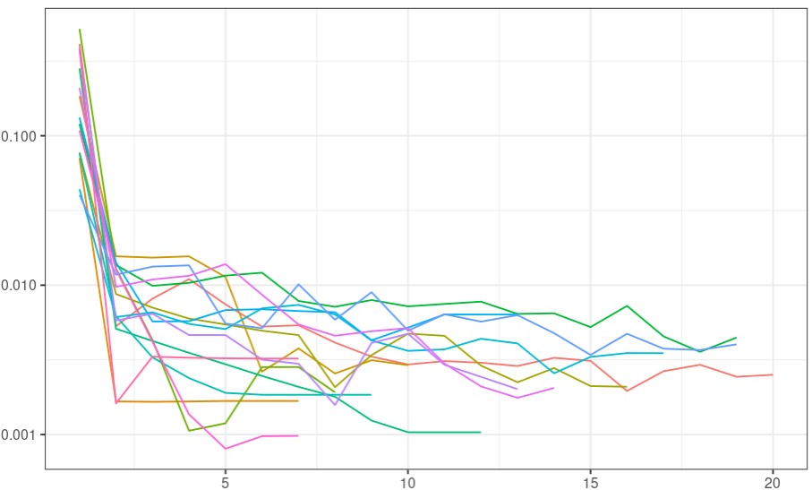
(a) Uniform case

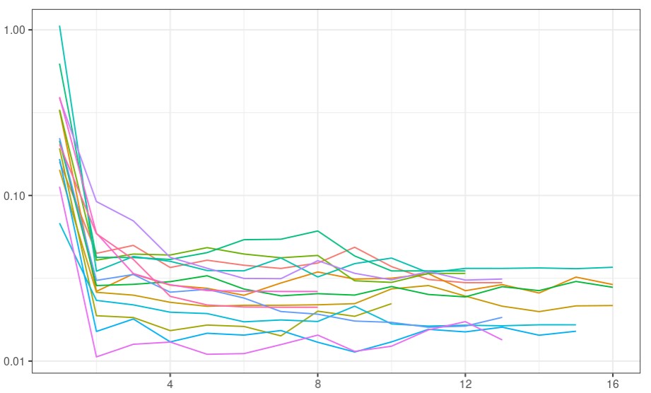
(b) Gaussian case

(c) Hybrid case

Figure 16: Evolution of the quantization error throughout the iterations over 15 experiment repetitions.

Appendix H Flooding prototype maps

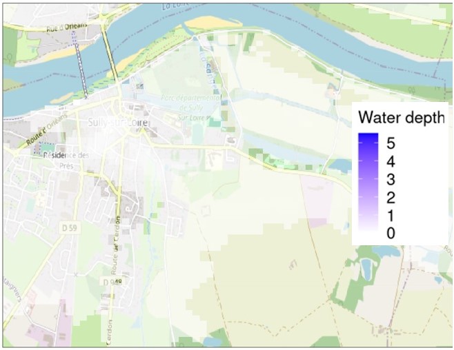
(a) $P=9.9\times 10^{-1}$

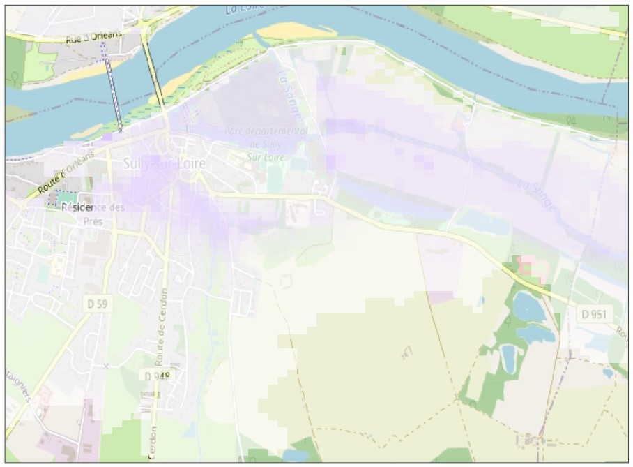
(b) $P=3.5\times 10^{-3}$

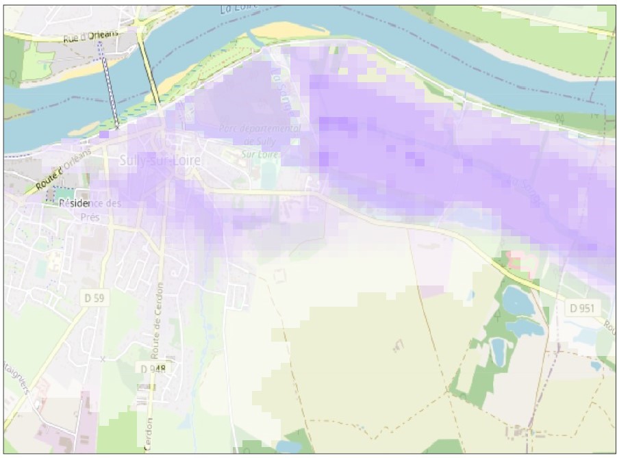
(c) $P=1.5\times 10^{-3}$

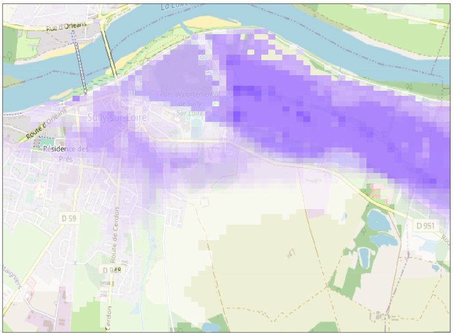
(a) $P=8.9\times 10^{-4}$

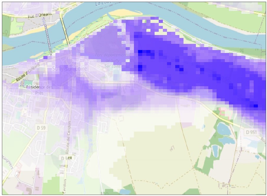
(b) $P=5.8\times 10^{-4}$

Figure 18: The 5 flooding prototype maps of the Loire case study. The map (e), corresponding to the most severe flooding, is the one chosen for the case study in the main body of the article. It defines a cluster of floodings whose inputs are analyzed through Augmented Quantization.

References

- [1] Murray Aitkin and Donald B. Rubin “Estimation and Hypothesis Testing in Finite Mixture Models” In Journal of the Royal Statistical Society. Series B (Methodological) 47.1 [Royal Statistical Society, Wiley], 1985, pp. 67–75 URL: http://www.jstor.org/stable/2345545
- [2] Brent Burch and Jesse Egbert “Zero-inflated beta distribution applied to word frequency and lexical dispersion in corpus linguistics” PMID: 35706513 In Journal of Applied Statistics 47.2 Taylor & Francis, 2020, pp. 337–353 DOI: 10.1080/02664763.2019.1636941
- [3] Marco Capó, Aritz Pérez and Jose A. Lozano “An Efficient Split-Merge Re-Start for the K-Means Algorithm” In IEEE Transactions on Knowledge and Data Engineering 34.4, 2022, pp. 1618–1627 DOI: 10.1109/TKDE.2020.3002926
- [4] O-Yeat Chan and Dante V. Manna “Congruences for Stirling Numbers of the Second Kind”, 2009
- [5] Sébastien Da Veiga, Fabrice Gamboa, Bertrand Iooss and Clémentine Prieur “Basics and trends in sensitivity analysis: Theory and practice in R” SIAM, 2021
- [6] Frank Dellaert “The Expectation Maximization Algorithm”, 2003
- [7] Qiang Du, M. Emelianenko and Lili Ju “Convergence of the Lloyd Algorithm for Computing Centroidal Voronoi Tessellations” In SIAM Journal on Numerical Analysis 44, 2006, pp. 102–119 DOI: 10.1137/040617364
- [8] Nicolas Fournier and Arnaud Guillin “On the rate of convergence in Wasserstein distance of the empirical measure”, 2013 arXiv:1312.2128 [math.PR]
- [9] R.M. Gray and D.L. Neuhoff “Quantization” In IEEE Transactions on Information Theory 44.6, 1998, pp. 2325–2383 DOI: 10.1109/18.720541
- [10] Stephen Joe and Frances Y Kuo “Notes on generating Sobol sequences” In ACM Transactions on Mathematical Software (TOMS) 29.1 Citeseer, 2008, pp. 49–57
- [11] Clément Levrard “Quantization/clustering: when and why does k-means work?” working paper or preprint, 2018 URL: https://hal.archives-ouvertes.fr/hal-01667014
- [12] Jean Maurin et al. “Études de dangers des digues de classe A de la Loire et de ses affluents – retour d’expérience”, 2013
- [13] Quentin Mérigot, Filippo Santambrogio and Clément Sarrazin “Non-asymptotic convergence bounds for Wasserstein approximation using point clouds” In Advances in Neural Information Processing Systems 34, 2021, pp. 12810–12821
- [14] See Ng, Thriyambakam Krishnan and G. Mclachlan “The EM algorithm” In Handbook of Computational Statistics: Concepts and Methods, 2004 DOI: 10.1007/978-3-642-21551-3˙6
- [15] Sloan Nietert, Ziv Goldfeld, Ritwik Sadhu and Kengo Kato “Statistical, Robustness, and Computational Guarantees for Sliced Wasserstein Distances” In Advances in Neural Information Processing Systems 35 Curran Associates, Inc., 2022, pp. 28179–28193 URL: https://proceedings.neurips.cc/paper_files/paper/2022/file/b4bc180bf09d513c34ecf66e53101595-Paper-Conference.pdf
- [16] OpenStreetMap contributors “Planet dump retrieved from https://planet.osm.org ”, https://www.openstreetmap.org, 2017
- [17] Gilles Pagès “Introduction to optimal vector quantization and its applications for numerics” 54 pages, 2014 URL: https://hal.archives-ouvertes.fr/hal-01034196
- [18] Victor M. Panaretos and Yoav Zemel “Statistical Aspects of Wasserstein Distances” In Annual Review of Statistics and Its Application 6.1, 2019, pp. 405–431 DOI: 10.1146/annurev-statistics-030718-104938
- [19] Lucie Pheulpin, Antonin Migaud and Nathalie Bertrand “Uncertainty and Sensitivity Analyses with dependent inputs in a 2D hydraulic model of the Loire River”, 2022 DOI: 10.3850/IAHR-39WC2521716X20221433
- [20] D. Pollard “Quantization and the method ofk-means” In IEEE Transactions on Information Theory 28.2, 1982, pp. 199–205 DOI: 10.1109/TIT.1982.1056481
- [21] Ludger Rueschendorf “The Wasserstein Distance and Approximation Theorems” In Probability Theory and Related Fields 70, 1985, pp. 117–129 DOI: 10.1007/BF00532240
- [22] Shokri Z. Selim and M.. Ismail “K-Means-Type Algorithms: A Generalized Convergence Theorem and Characterization of Local Optimality” In IEEE Transactions on Pattern Analysis and Machine Intelligence PAMI-6.1, 1984, pp. 81–87 DOI: 10.1109/TPAMI.1984.4767478
- [23] Charlie Sire “The FunQuant package” In GitHub repository GitHub, 2023 URL: https://github.com/charliesire/FunQuant
- [24] Charlie Sire et al. “Quantizing rare random maps: application to flooding visualization” In Journal of Computational and Graphical Statistics 0 Taylor & Francis, 2023, pp. 1–31 DOI: 10.1080/10618600.2023.2203764
- [25] Ramesh Sridharan “Gaussian mixture models and the EM algorithm”, 2014
- [26] Onur Teymur, Jackson Gorham, Marina Riabiz and Chris Oates “Optimal Quantisation of Probability Measures Using Maximum Mean Discrepancy”, 2020
- [27] C. Villani “Optimal Transport: Old and New”, Grundlehren der mathematischen Wissenschaften Springer Berlin Heidelberg, 2016 URL: https://books.google.fr/books?id=5p8SDAEACAAJ
- [28] Sidney J. Yakowitz and John D. Spragins “On the Identifiability of Finite Mixtures” In The Annals of Mathematical Statistics 39.1 Institute of Mathematical Statistics, 1968, pp. 209–214 DOI: 10.1214/aoms/1177698520