Non-LTE abundance analysis of A-B stars with low rotational velocities. II. Do A-B stars with normal abundances exist?

Abstract

We present chemical composition and fundamental parameters (the effective temperature, surface gravity and radius) for four sharp-lined A-type stars $\gamma$ Gem (HD 41705), $o$ Peg (HD 214994), $\theta$ Vir (HD 114330) and $\nu$ Cap (HD 193432). Our analysis is based on a self-consistent model fitting of high-resolution spectra and spectrophotometric observations over a wide wavelength range. We refined the fundamental parameters of the stars with the SME  package and verified their accuracy by comparing with the spectral energy distribution and hydrogen line profiles. We found $T_{\rm eff}$/$\log{g}$  = 9190$\pm$130 K/3.56$\pm$0.08, 9600$\pm$50 K/3.81$\pm$0.04, 9600$\pm$140 K/3.61$\pm$0.12, and 10200$\pm$220 K/3.88$\pm$0.08 for $\gamma$ Gem, $o$ Peg, $\theta$ Vir  and $\nu$ Cap, respectively. Our detailed abundance analysis employs a hybrid technique for spectrum synthesis based on classical model atmospheres calculated in local thermodynamic equilibrium (LTE) assumption together with the non-LTE (NLTE) line formation for 18 of 26 investigated species. Comparison of the abundance patterns observed in A stars of different types (normal A, Am, Ap) with similar fundamental parameters reveals significant abundance diversity that cannot be explained by the current mechanisms of abundance peculiarity formation in stellar atmospheres. We found a rise of the heavy element (Zn, Sr, Y, Zr, Ba) abundance excess up to +1 dex with $T_{\rm eff}$ increasing from 7200 to 10000 K, with a further decrease down to solar value at $T_{\rm eff}$ = 13000 K, indicating that stars with solar element abundances can be found among late B-type stars.

1 Introduction

The chemically peculiar stars of spectral types from A to middle B are known for various types of chemical anomalies. They include both chemically-peculiar magnetic (Ap SiSrCrEu type) and non-magnetic (Hg-Mn type) stars as well as stars with moderately enhanced metalic lines (Am) and weakened metalic lines ($\lambda$ Boo type).

The chemical anomalies in peculiar stars are of great interest for studying and understanding the physics of processes in the interiors of stars. It is believed that the origin of the chemical anomalies is connected with the atomic diffusion processes. To explain the observed anomalies, Michaud (1970) proposed a theory of diffusion, according to which the diffusion of atoms and ions of an element occurs under the action of gravity directed towards the centre of the star and radiation pressure forces pushing particles into the outer layers of the atmosphere.

To explain the Am star phenomenon two different atomic diffusion scenarios are proposed. Watson (1971) suggested that the separation of chemical elements occurs directly below the hydrogen convection zone, in the radiative zone (see e.g. Alecian, 1996) and it is assumed that a very small mass of a star gets high abundance when the star is on the main sequence (MS) stage. Further, when the star reaches the subgiant branch, a decrease in abundances in the star’s atmosphere is assumed. In another model proposed by Richer et al. (2000), the separation of elements occurs much deeper in the star. Consequently, larger part of stellar mass gets an anomalous chemical composition when the star is in the MS stage and, further, the anomalies remain presumably longer as the star evolves to the subgiant stage.

To understand the mechanisms of formation of chemical element anomalies, accurate elemental abundance determinations from light CNO to the rare earth elements (lanthanides) are required for each group of chemically peculiar stars. Observations (Preston, 1974) and theory (Michaud, 1982) show that slow rotation (equatorial velocity below 120 km s^-1) favours the presence of chemical anomalies in hot A-B stars. Mashonkina et al. (2020, hereafter, Paper  i) carried out a detailed analysis of the atmospheres of a sample of slowly rotating A-B stars with effective temperatures mostly above 9300 K. Abundances of 14 chemical elements from He to Nd were determined taking into account deviations from the local thermodynamic equilibrium (NLTE approach). Both Am and normal A stars have an excess of heavy elements Sr-Zr-Ba-Nd compared to the solar abundance, with Ba having the maximum excess among them. An increase in the abundance of heavier elements seems to correlate with an increase in the effective temperature in hot stars.

In this study we aim to complement the stellar sample of Mashonkina et al. (2020) with effective temperature range from 9000 to 11000 K with a detailed chemical element abundances determined in LTE and NLTE, where available. This sample includes four A-B stars: $\gamma$ Gem (HD 47105, Alhena), $o$ Peg (HD 214994), $\theta$ Vir (HD 114330), and $\nu$ Cap (HD 193432). Abundances of 26 elements were obtained with the NLTE treatment for 18 of them.

The paper is organised as follows. Section 2 provides information about sample stars observations used in our study. The methods and the results of the atmospheric parameter determinations are given in Section 3. In Section 4 we provide the results of abundance analysis. Comparison of our abundance results with those from the literature for the sample stars is given in Section 5. Evolutionary status of the sample stars is considered in Section 6. We compare abundance patterns of different types of A stars (normal A, Am, Ap) with close atmospheric parameters and evolutionary status in Section 7. Discussion and conclusions are presented in Section 8.

2 Stellar sample and observations

2.1 Stellar sample

$\gamma$ Gem  is a well known spectroscopic binary star, where the A component Alhena A has an extremely small surface magnetic field of 30 G (Blazère et al., 2020). The mass of the primary is 2.8 $M_{\odot}$. The secondary component is 5 - 6 mag fainter than the primary star and it has a mass of 1.07 $M_{\odot}$ (Fekel & Tomkin, 1993). It was classified as a cool G star (Thalmann et al., 2014). The primary was classified as a normal A type star, but with higher abundances of Zr, Ba, La, Ce, and Nd compared to solar values, and it lies somewhere between a normal A star and Am star (Adelman et al., 2015b). SIMBAD database contains data on fundamental parameters obtained through different methods. The effective temperature ($T_{\rm eff}$) ranges from 8900 K to 10700 K, while the surface gravity ($\log{g}$) spans from 3.46 to 4.00.

$o$ Peg  was identified as a low-amplitude, long-period binary with the spectral type of the primary A1 IV. The mass function is $f(m)$ = 0.00066 $\pm$ 0.00024 $M_{\odot}$ (Fekel, 1999). There is no information about mass and spectral type of the secondary component, but we expect its mass to be much smaller than that of the primary star. SIMBAD provides the effective temperature in the range of 8300 K to 10080 K, and the surface gravity is given within the range of 3.20 to 4.00. No significant polarisation signal was detected in course of the highly sensitive search for magnetic fields in B, A and F stars (Shorlin et al., 2002), providing an estimate -32$\pm$20 G for the longitudinal magnetic field.

$\theta$ Vir  was identified as A1 IV spectral type double or multiple star. According to Washington Double Star (WDS) catalog (Mason et al., 2001). $\theta$ Vir is a multiple system containing four components. Two of them are displayed at a distance of $7^{\prime\prime}$ and $71^{\prime\prime}$ from the main component. The main star is an interferometric binary with a separation of $\sim 0.4^{\prime\prime}$ (McAlister & Hendry, 1982) and magnitude difference of $2.2^{m}$ (ten Brummelaar et al., 2000). Mass estimates of 2.98 and 0.08 $M_{\odot}$ are given in Schwarz et al. (2009) for both components, respectively. The contribution of the secondary component to the spectrum may be not negligible, however, the star was included in the list of CALSPEC spectrophotometric standards (Rubin et al., 2022). Finally, we ignored the possible effect of a close secondary component on the common spectra of sample stars and on the spectral energy distributions in our analysis.

$\nu$ Cap  is a superficially normal single star with B9 IV spectral type. The elemental abundances of $\nu$ Cap  was recently analysed in (Monier et al., 2018) and (Adelman, 1991), but non-LTE effects were neglected. The effective temperature is given in SIMBAD in the range of 9690–10900 K, and the surface gravity is given as 3.00–4.00.

Part of the literature data on the fundamental parameters of the program stars is given in Table 1. It is important to note that the majority of the previous abundance studies were conducted in LTE. Here and throughout the paper, an error in the measurement of the last digits is given in parentheses.

Table 1: Literature data on the fundamental parameters of the program stars.

Star	$T_{\rm eff}$	$\log{g}$	Reference	Method
$\gamma$ Gem	8953	3.46	Gray et al. (2003)	Spectrophotometry
	9040(280)		Zorec et al. (2009)	Spectrophotometry
	9150(100)	3.60(10)	Adelman et al. (2002)	Spectroscopy
	9341		Di Benedetto (1998)	Photometry
	9440	3.59	Hill & Landstreet (1993)	Spectroscopy
$o$ Peg	9373(303)	3.73(23)	Prugniel et al. (2011)	Spectroscopy
	9575(15)	3.73(01)	Adelman et al. (2015b)	Spectroscopy
	9680	3.71	Hill & Landstreet (1993)	Spectroscopy
	9720		Di Benedetto (1998)	Photometry
	9930(350)		Zorec et al. (2009)	Spectrophotometry
$\theta$ Vir	9500	3.60	Dobrichev et al. (1987)	Spectroscopy
	9509	3.80	Cenarro et al. (2007)	Spectroscopy
	9570(264)	3.95(11)	Prugniel et al. (2011)	Spectroscopy
	9671(289)	3.57(82)	Koleva & Vazdekis (2012)	Spectroscopy
$\nu$ Cap	10250	3.90	Adelman (1991)	Spectrophotometry
	10185	3.88	Erspamer & North (2003)	Photometry
	10300(250)	3.90(25)	Monier et al. (2018)	Photometry

2.2 Observations

For the sample stars, we used spectra taken with different instruments, selecting the highest quality spectrum available in the archives for each star. For $\gamma$ Gem, spectroscopic observations were extracted from the FEROS spectrograph (MPG/ESO 2.2-metre telescope, La Silla) archive and cover the spectral range of 3500-9200 Å  (program ID – 082.A-9007, PI – J. Carson, SNR$\simeq$430). The resolving power of the instrument is $R=\lambda/\delta\lambda=48\,000$. For $o$ Peg, we used spectra from ESPaDOnS spectrograph (Canada-France-Hawaii Telescope) archive covering the spectral range 3700-10500 Å  with $R=68\,000$ (proposal ID – 14AC03, PI – V. Khalack). Twelve spectra were averaged providing the final SNR$\approx$700. For $\theta$ Vir, we found available observations taken with the HARPS spectrograph (High Accuracy Radial velocity Planet Searcher) archive (3000-10000 Å, $R=80\,000$, program ID – 60.A-9709(G), SNR$\simeq$250) and we also used ESPaDOnS spectrum for the near infrared (IR) range (proposal ID – E02, PI – N. Manset). For $\nu$ Cap, spectral observations taken with the UVES spectrograph were extracted from the ESO archive (programs ID – 67.D-0384(A), PI – J. Orosz; 076.D-0169(A), PI – Ch. Cowley). Spectra cover 3730-6835 Å wavelength range with $R=37\,000$, SNR$\simeq$150, and 5650-9460 Å wavelength range with $R=107\,000$ and SNR$\simeq$250. The last spectrum was used for nitrogen and oxygen abundance determination.

Photometric and spectrophotometric observations in different spectral regions were employed to construct the spectral energy distribution (SED) for each star. For the ultraviolet (UV) region, we used observations obtained with the S2/68 telescope of TD1 mission (European Space Research Organization (ESRO) satellite), which measured the absolute flux in four bands, 1565 Å, 1965 Å, 2365 Å, and 2740 Å  (Thompson et al., 1978), and spectra from the International Ultraviolet Explorer (IUE) obtained through the large aperture. In the optical range, we used data from Adelman’s spectrophotometric catalogue (Adelman et al., 1989). Photometric data in the IR region were taken from the 2Micron All-Sky Survey (2MASS, Cutri et al., 2003), which contains an overview of the entire sky in J (1.25 $\mu$m), H (1.65 $\mu$m), and Ks (2.17 $\mu$m) filters. Observations were transformed into the absolute fluxes using the calibrations given in Cohen et al. (2003).

3 Stellar fundamental parameters

3.1 SME

Fundamental parameters of sample stars were determined using SME  (Spectroscopy Made Easy) spectral package (Valenti & Piskunov, 1996; Piskunov & Valenti, 2017). It computes synthetic spectra in a given spectral regions taking into account all possible blends, performs fit to the observed spectra, and finds best-fit solution for the atmospheric parameters $T_{\rm eff}$, $\log{g}$, apparent rotation velocity ($v_{\rm e}\sin i$), microturbulent velocity ($\xi_{\rm t}$), macroturbulent velocity ($\zeta_{\rm RT}$), and metallicity ([M/H]) within the grids of model atmospheres. SME  enables a careful selection of spectral features that exhibit sensitivity to different atmospheric parameters (line mask). These parameters are the free parameters of the fit. The present study is based on LLmodels grid (Shulyak et al., 2004). SME masks are constructed in wide spectral regions 4250–6700 Å ($o$ Peg, $\theta$ Vir, $\nu$ Cap), 4400–6460 Å ($\gamma$ Gem). Our masks include from three (H$\gamma$, H$\beta$, H$\alpha$) to one (H$\beta$) hydrogen lines, which are sensitive to $T_{\rm eff}$ and, especially $\log{g}$ variations, in the range of stellar parameters we are interested in. The masks also contain $\approx$300 lines of Fe i and Fe ii of different excitation energies with the equivalent widths (EW) from 3 to 110 mÅ in order to refine $T_{\rm eff}$ and $\log{g}$ via excitation and ionisation equilibria as well as to determine $\xi_{\rm t}$.

The uncertainties of the free parameters are estimated with two methods: the first one is the classical method derived from the covariance matrix of the least square fitting procedure, while the second method is based on the analysis of cumulative probability distribution for each parameter (see Ryabchikova et al., 2016; Piskunov & Valenti, 2017; Wehrhahn et al., 2023, for more details) and it includes the residuals of the fit that also reflect systematic errors such as detector defects, continuum normalisation, missing or erroneous atomic data, etc. The distribution for each free parameter consists of the changes to this parameter that are needed to achieve a perfect fit (zero residual) in every spectral point. Only points sensitive to the parameter in question are included. Central part of the distribution for each parameter is close to Gaussian with the uncertainty depending on the point statistics and it can be used to determine the median and the width of the distribution in the integral form (cumulative distribution). Every free parameter is treated independently and so this approach tends to overestimate the uncertainty if statistics is poorly sampled, which becomes the case when only a small number of spectral points in chosen regions is sensitive to the parameter. When statistics is good this method provides reasonable error estimates for free parameters that affect the majority of spectral points (e.g. $T_{\rm eff}$, [M/H]). The true values of uncertainties of the free parameters lies somewhere in between the two estimates.

3.2 SED

To check the accuracy of the fundamental parameters determination, we used spectral energy distribution (SED). When calculating the SED for all stars except $\nu$ Cap, the value of $\log{g}$  was taken from the SME  solution and fixed in the fitting procedure. For $\nu$ Cap we derived same temperatures with fixed and not fixed $\log{g}$. For each star, we constructed a set of observed fluxes using the data described in Section 2.2. For $\gamma$ Gem, we used the UV data from the IUE and TD1 missions, in the optical range we used Adelman’s spectrophotometry, and 2MASS photometric measurements in the IR. For $o$ Peg, $\theta$ Vir, and $\nu$ Cap, the photometric and spectrophotometric data were taken from the IUE, TD1, Adelman’s, and 2MASS catalogues. Sample stars are nearby objects located within 100 pc, however, we accounted for the interstellar absorption in flux calculations. The correction for the interstellar reddening was applied according to extinction curve from Fitzpatrick (1999) with $A_{v}=3.1*E(B-V)$. All values of $E(B-V)$ were taken from the dust map given by Lallement et al. (2014). The corresponding $A_{v}$ are 0.04, 0.01, 0.0 and 0.01 for $o$ Peg, $\theta$ Vir, $\gamma$ Gem, and $\nu$ Cap, respectively.

3.3 Results

The fundamental parameters for all sample stars are presented in Table 2. For SME parameters, uncertainties estimated by the two methods are given, while the $T_{\rm eff}$ uncertainty from SED determination is obtained by the first classical method mentioned above.

Table 2: Fundamental parameters of the program stars derived in the present study.

Star name	$T_{\rm eff}$, K	$\log{g}$	[Fe/H]	$\xi_{\rm t}$, km s-1	$\zeta_{\rm RT}$, km s-1	$v_{\rm e}\sin i$, km s-1	$R/R_{\odot}$	$L/L_{\odot}$	Parallax, mas	Method
$\gamma$ Gem	9100$\pm$10	3.60					5.16$\pm$0.77	2.21$\pm$0.13	29.84*	SED
	9190$\pm$20$\pm$130	3.56$\pm$0.01$\pm$0.08	0.06$\pm$0.01$\pm$0.08	1.77$\pm$0.03$\pm$0.36	5.43$\pm$0.65$\pm$3.93	10.59$\pm$0.23$\pm$1.71				SME
$o$ Peg	9550$\pm$10	3.80					3.37$\pm$0.10	1.93$\pm$0.03	11.65**	SED
	9600$\pm$10$\pm$50	3.81$\pm$0.01$\pm$0.04	0.25$\pm$0.01$\pm$0.09	1.98$\pm$0.04$\pm$0.32	5.20$\pm$0.64$\pm$2.34	5.40$\pm$0.49$\pm$1.11				SME
$\theta$ Vir	9660$\pm$20	3.60					4.03$\pm$0.30	2.10$\pm$0.07	11.18**	SED
	9600$\pm$10$\pm$140	3.61$\pm$0.01$\pm$0.12	0.15$\pm$0.01$\pm$0.14	1.42$\pm$0.01$\pm$0.62	3.78$\pm$0.03$\pm$1.52	0.10$\pm$2.26$\pm$7.80				SME
$\nu$ Cap	10160$\pm$10	3.95$\pm$0.08					3.04$\pm$0.08	1.95$\pm$0.02	12.17**	SED
	10200$\pm$10$\pm$220	3.88$\pm$0.01$\pm$0.08	0.08$\pm$0.01$\pm$0.14	0.96$\pm$0.02$\pm$0.55	0.00	22.85$\pm$0.04$\pm$2.56				SME

Note. *van Leeuwen (2007); **Gaia Collaboration (2020)

For $\gamma$ Gem, we obtained $T_{\rm eff}$  = 9190 K and $\log{g}$  = 3.56 from SME. From SED we derived $T_{\rm eff}$  = 9100 K (Fig. 1). However, as in the case of the magnetic star HD 108662 (see Romanovskaya et al., 2020), it turned out that there is a noticeable disagreement in the narrow spectral region between the UV and optical observations. A good agreement between the observed and theoretical energy distribution could only be obtained assuming a scaling factor of 1.05 for the IUE flux and TD1 photometry.

For $o$ Peg, we obtained $T_{\rm eff}$ = 9600 K, $\log{g}$ = 3.81 from SME, and $T_{\rm eff}$  = 9550 K from SED  (see Fig. 9 in Appendix). In this case we keep assuming a scaling factor of 1.05 for the IUE flux and TD1 photometry with the same reasons as for $\gamma$ Gem.

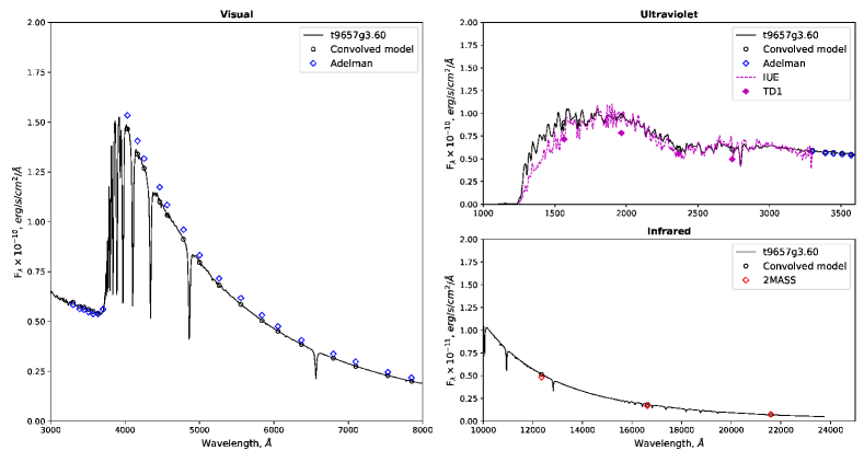
Figure 10: Spectral energy distribution of $\theta$ Vir  in the UV, visual and IR spectral regions. Black solid line shows theoretical SED  calculation with the model atmosphere parameters t9657g36.

For $\theta$ Vir, atmospheric parameters from SME  are $T_{\rm eff}$ = 9600 K, $\log{g}$ = 3.61 and SED  gives $T_{\rm eff}$ = 9660 K (see Fig. 10 in Appendix).

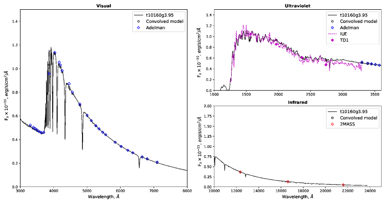
Figure 11: Spectral energy distribution of $\nu$ Cap  in the UV, visual and IR spectral regions. Black solid line shows theoretical SED  calculation with the model atmosphere parameters t10160g395.

For $\nu$ Cap, we obtained $T_{\rm eff}$ = 10200 K, $\log{g}$ = 3.88 from SME  analysis and $T_{\rm eff}$ = 10150 K from SED  fitting (see Fig. 11 in Appendix).

For each program stars, the atmospheric parameters derived from spectroscopic and spectrophotometric observations agree well within the error limits.

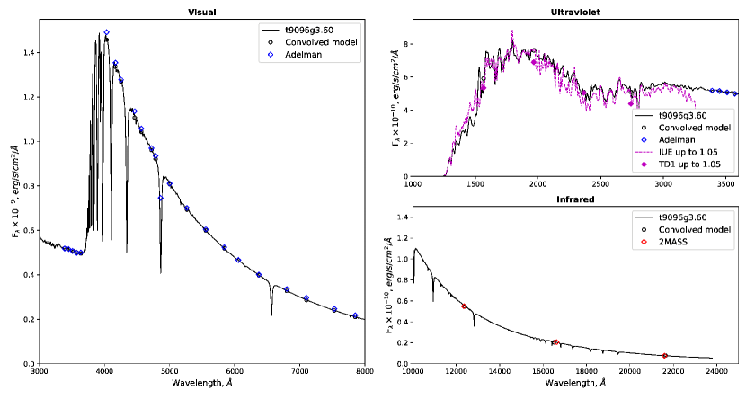
Figure 1: Spectral energy distribution of $\gamma$ Gem  in the UV, visual, and IR spectral regions with Adelman’s photometry data points. Black solid line shows theoretical SED  calculation with the model atmosphere parameters $T_{\rm eff}$ = 9096 K, $\log{g}$ = 3.6. IUE and TD1 points were raised by a factor of 1.05.

Along with the $T_{\rm eff}$  and $\log{g}$, the microturbulent velocity is another parameter that affects abundances. It is adjusted in a such way that, for a given species, spectral lines of different equivalent width yield similar abundances. We checked $\xi_{\rm t}$  obtained from SME  for $\gamma$ Gem  (see Fig. 2) by manually fitting the individual spectral line profiles of Fe i and Fe ii  lines (see Section 4) and found that the $\xi_{\rm t}$ found in SME meets the above criteria. The same is true for $o$ Peg, $\theta$ Vir, and $\nu$ Cap.

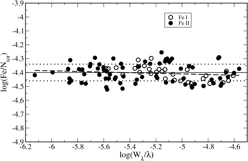
Figure 2: Abundances from Fe  i (open circles) and Fe ii (filled circles) lines in $\gamma$ Gem  versus the reduced equivalent widths. Solid and dashed lines represent an average Fe abundance and regression line of the entire set, correspondingly. The uncertainty limits are shown by dotted lines.

4 Abundance analysis

Abundance analysis was carried out with the model atmospheres obtained from SME. For each chosen line, abundance is determined by fitting the synthetic line profile to the observed profile using the code SynthVb  (Tsymbal et al., 2019) along with the code BinMag6 (Kochukhov, 2018), which may implement the pre-computed departure coefficients (the ratio of NLTE to LTE atomic level populations). For elements up to Ba, the abundances were obtained from the lines of the neutral atoms and first ions, while for the rare-earth elements (REE), we used the lines of the first and second ions.

Element abundances are given in a standard designation, $\log\varepsilon$ = $\log(N_{\rm El}/N_{\rm H})$ + 12, where N_El and N_H are number densities of a given chemical element and hydrogen, respectively. For each star, the full linelist with the line atomic parameters and individual line abundances is available online (see Section Data Availability for details). Part of the list, for guidance, is given in Table 3.

Table 3: The linelist of LTE and NLTE abundances from individual lines in program stars together with the line atomic parameters and the references to them.

				References			Abundances, $\log\varepsilon$
							$\gamma$ Gem		$o$ Peg		$\theta$ Vir		$\nu$ Cap
Ion	Wavelength, Å	$E_{i}$, eV	log$gf$	gf	HFS	IS	LTE	NLTE	LTE	NLTE	LTE	NLTE	LTE	NLTE
. . .
He 1	4471.4730	20.9641	-0.2780	WSG	-	-	10.93	10.90	10.89	10.87	10.71	10.69	10.96	10.95
He 1	5875.6150	20.9641	0.4090	WSG	-	-	11.02	10.92	10.93	10.86	10.89	10.81	11.01	10.94
. . .
Ba 2	4554.0319	0.0000	0.1700	MW	BBW/VAHW	WABM	2.64	2.92	3.44	3.62	3.19	3.49	2.76	3.09
Ba 2	4934.0750	0.0000	-0.1500	MW	BWE-BBW/VAHW	WABM	2.65	2.94	3.40	3.61	3.18	3.49	2.79	3.11
Ba 2	5853.6742	0.6043	-1.0000	MW	VBDSb/VAHW	VBDS	2.84	3.14	3.45	3.69	3.28	3.61	-	-
. . .

Note. This table is available in its entirety in a machine-readable form in the online journal. A portion is shown here for guidance regarding its form and content. References of HFS constants are given for lower and upper levels. WSG = Wiese et al. (1966); MW = Miles & Wiese (1969); BBW = Becker et al. (1981); VAHW = Villemoes et al. (1993); WABM = Wendt et al. (1984); BWE = Blatt & Werth (1982); VBDSb = van Hove et al. (1985); VBDS = Van Hove et al. (1982).

For most chemical elements, we determined NLTE abundances, while Sc, V, Cr, Mn, Co, Ni, La, Nd abundances are determined in LTE.

For C i – ii, O i, Na i, Mg i – ii, Si i – ii, K i, Ca i – ii, Ti i – ii, Fe i – ii, Zn i – ii, Sr ii, Y ii, Zr ii – iii, and Ba ii, the NLTE calculations are performed with a modified version of the DETAIL code (Giddings, 1981; Butler, 1984) with the opacity package updated by Przybilla et al. (2011). For He i, N i – ii, Al i, and S i, NLTE calculations are performed with the MULTI code (Carlsson, 1986) where the opacity calculation block was replaced with that from ATLAS9 (Castelli & Kurucz, 2003) as described by Korotin et al. (1999). We are using two NLTE codes because model atoms for some species are created for a specific code. However, we have compared NLTE calculations with DETAIL and MULTI codes for common elements Na i  and Mg i in $\gamma$ Gem. The derived abundance difference between two NLTE codes does not exceed 0.03 dex which is comparable to the uncertainty of NLTE abundance determinations.

The NLTE abundances of He, C, O, Na, Mg, Si, Ca, Ti, Fe, Sr, Zr, and Ba are determined using the same NLTE methods as in Paper  i and we refer the reader to that study. In addition to the list of chemical elements investigated in Paper  i, here we also determine NLTE abundances of N, Al, S, K, Zn, Y in the four sample stars and the comparison stars from Paper  i (HD 32115, 21 Peg, Sirius, and HD 72660). For these elements, their abundance determination methods are described below. The derived abundances for the sample stars are presented in Table 4, while our results for comparison stars are given in Table 5

Nitrogen NLTE calculations were performed with the model atom originally described by Lyubimkov et al. (2011) and modified by Andrievsky et al. (2021). This model was supplemented by the detailed calculations of low-energy inelastic collisions with hydrogen atoms (Amarsi & Barklem, 2019). Twenty so-called super levels of N i and transitions between them were added in order to reliably describe the relationship between the excited levels of neutral nitrogen and the continuum. Seventy-five highly excited N i levels were combined in 20 super levels according to their parity. In total, the model atom contains 59 N i levels, 49 N ii levels, N iii ground state, and more than 900 b-b transitions between them.

In $\gamma$ Gem  and $o$ Peg, we determined nitrogen NLTE abundances $\log\varepsilon$ = 7.74$\pm$0.07 and 8.05$\pm$0.06, respectively. Our results agree with the NLTE determinations of Takeda et al. (2018), who found $\log\varepsilon$ = 7.74 and 8.00, from analysis of the single N i 7468 Å line in the same stars. For Sirius and $\nu$ Cap, we found 0.23 dex and 0.18 dex lower abundances compared to those of Takeda et al. (2018). Both stars have the largest projected rotational velocities among the program and the comparison stars. Abundance analysis of Takeda et al. (2018) was based on EW measurements, therefore partially this difference may be attributed to a small blend of S  i 7868.59 Å line, which may affect the total EW in a different way in stars with different rotational velocity.

Aluminium The two resonance Al i lines and several Al ii lines are suitable for abundance determination, but the resonance lines are strongly affected by NLTE. For NLTE calculations we used the Al i model atom described in details in Andrievsky et al. (2021) and modified by Caffau et al. (2019). This model atom consists of 76 levels of Al i and 13 levels of Al ii and it takes into account about 300 b-b transitions between them. NLTE effects lead to a significant weakening of the resonance lines and the NLTE corrections reach 0.40 dex in the stars under study. High-excitation Al ii lines were considered in LTE approximation. For the four sample stars, the abundance difference between Al i and Al ii varies from 0.03 to 0.17 dex in different stars. We consider this result to be satisfactory, due to possible uncertainties in NLTE calculations for Al i resonance lines caused by their position in the wing of the strong Ca ii 3933 Å resonance line.

Sulfur NLTE calculations for S i were performed with the model described in details in Korotin (2009). The model atom includes 64 levels of singlet, triplet and quintet systems of S i, the ground level of S ii and about 400 radiative transitions between them. In our analysis, transition probabilities for S i and S ii lines are taken from Zatsarinny & Bartschat (2006) and Irimia & Fischer (2005), respectively. NLTE corrections for the S i lines adopted for abundance determination in this study are small in the temperature domain of our sample stars. They can be either positive or negative and range from –0.04 to +0.10 dex. However, the IR lines of the S i 9221-9237 Å triplet are always strengthened due to NLTE effects, and their NLTE abundance corrections range from –0.5 to –0.8 dex.

For S ii lines, we performs LTE analysis. For the four stars where lines of S i and S ii are both measured, we found NLTE abundances from S i to be systematically higher compared to S ii, with the abundance difference from 0.6 to 0.24 dex. Partially, the difference of  0.2 dex is probably caused by the uncertainty in theoretical transition probabilities, which is  0.15 dex according to NIST (Kramida et al., 2022).

Potassium We apply a comprehensive model atom of K i developed by Neretina et al. (2020) using the most up-to-date atomic data on energy levels (46 levels with a principal quantum number $n\leq 14$), transition probabilities, photoionisation cross-sections, and electron-impact excitation rates. Singly-ionised potassium is represented by the ground state only because the first excited level has an excitation energy of 20.2 eV.

Zinc NLTE calculations for Zn are performed with a Zn i – ii model atom of Sitnova et al. (2022). It includes 28 levels of Zn i, 7 levels of Zn ii, and the ground state of Zn iii. This model atom employs photoionisation cross-sections from the R-matrix calculations of Liu et al. (2011) and electron impact excitation cross sections from the R-matrix calculations of Zatsarinny & Bartschat (2005). In our sample stars, NLTE leads to higher Zn abundances compared to LTE.

Yttrium We construct a model atom for Y ii using atomic level energies and oscillator strengths from calculations of R. Kurucz available on his web-page. Our Y ii model atom includes 94 levels of Y ii and the ground state of Y iii. Energy levels with E${}_{exc}>$ 10 eV are combined in 22 super levels according to their parity. For electron impact excitation and ionisation and photoionisation we use approximate formulae to calculate the transition rates. Namely, hydrogenic formula with an effective principal quantum number for photoionisation, Seaton (1962) formula for electron impact ionisation, and van Regemorter (1962) and Woolley & Allen (1948) formulae for electron-impact excitation for radiatively allowed and forbidden transitions, respectively. To estimate the accuracy of our NLTE results, we perform test calculations with scaling electronic collision rates and photoionisation cross sections by one order of magnitude. For the investigated lines, an application of ten times smaller photoionisation rates or ten times larger electron impact ionisation rates does not affect the NLTE abundances, while ten times increase in electron collision excitation rates results in significantly smaller departures from LTE. For example, for Sirius, the latter test calculations result in up to 0.1 dex lower NLTE abundances compared to that derived with the standard rates. The effect is different for different spectral lines: it is small for Y ii lines in the UV spectral range and reaches maximum for the strongest lines in the visible spectrum.

In atmospheres of A-type stars, Y ii is the minority species. For example, in Sirius, the number density of Y ii is an order of magnitude smaller compared to that of Y iii in the line formation layers. The mechanism of the departures from LTE is driven by an overionisation and results in a higher abundance compared to LTE. This effect increases with $T_{\rm eff}$. For the hottest sample stars, NLTE results in up to 0.5 dex higher average abundance compared to LTE. An exception is the coolest F-type star HD 32115, where Y ii dominates and has small negative NLTE abundance corrections.

Table 4: Average NLTE and LTE chemical element abundances in the program stars.

Ion		$\gamma$ Gem			$o$ Peg			$\theta$ Vir			$\nu$ Cap			Sun
		$\log\varepsilon$	[X/H]	nl	$\log\varepsilon$	[X/H]	nl	$\log\varepsilon$	[X/H]	nl	$\log\varepsilon$	[X/H]	nl	$\log\varepsilon$
He i	L	10.94(05)	0.016	4	10.89(03)	-0.034	4	10.80(08)	-0.124	3	10.98(03)	0.056	4	10.924
He i	N	10.90(01)	-0.024	4	10.88(03)	-0.044	4	10.76(05)	-0.164	3	10.94(01)	0.016	4
C i	L	8.50(09)	0.03	9	8.08(12)	-0.39	11	8.28(13)	-0.19	8	8.30(11)	-0.17	4	8.47
C i	N	8.48(08)	0.01	9	8.13(10)	-0.34	11	8.35(09)	-0.12	8	8.41(09)	-0.06	4
N i	L	8.12(09)	0.27	10	8.43(15)	0.58	19	8.01(06)	0.16	15	8.20(08)	0.35	10	7.85
N i	N	7.74(07)	-0.11	10	8.05(06)	0.20	19	7.55(05)	-0.30	15	7.67(09)	-0.18	10
O i	L	9.13(53)	0.40	15	8.86(44)	0.13	18	8.99(53)	0.26	12	8.76(09)	0.03	13	8.73
O i	N	8.73(04)	0.00	15	8.55(07)	-0.18	18	8.55(03)	-0.18	12	8.67(07)	-0.06	13
Na i	L	6.95(26)	0.68	4	6.99(29)	0.72	5	6.75(28)	0.48	4	6.71(20)	0.44	3	6.27
Na i	N	6.41(03)	0.14	4	6.59(03)	0.32	5	6.36(02)	0.09	4	6.36(03)	0.09	3
Mg i	L	7.79(19)	0.27	6	7.62(14)	0.10	7	7.67(20)	0.15	11	7.67(13)	0.15	6	7.52
Mg i	N	7.66(04)	0.14	6	7.55(04)	0.03	7	7.54(02)	0.02	11	7.57(03)	0.05	6
Mg ii	L	7.65(14)	0.13	6	7.61(17)	0.09	9	7.53(10)	0.01	10	7.57(14)	0.05	4
Mg ii	N	7.62(08)	0.10	6	7.53(10)	0.01	9	7.46(06)	-0.06	10	7.53(07)	0.01	4
$\textnormal{[Mg/H]}_{mean}$	N	0.12(06)			0.02(07)			-0.02(05)			0.03(05)
Al i	L	6.17(05)	-0.25	2	6.51(05)	0.09	2	6.32(02)	-0.10	2	6.15(11)	-0.27	2	6.42
Al i	N	6.54(02)	0.12	2	6.90(04)	0.48	2	6.65(01)	0.23	2	6.44(09)	0.02	2
Al ii	L	6.46(09)	0.04	3	6.80(04)	0.38	4	6.48(10)	0.06	3	6.41(07)	-0.01	3
$\textnormal{[Al/H]}_{mean}$		0.12(07)			0.48(04)			0.23(01)
Si i	L	7.29(23)	-0.22	2	7.35(18)	-0.16	2	7.44(09)	-0.07	2				7.51
Si i	N	7.64(15)	0.13	2	7.65(11)	0.14	2	7.66(20)	0.15	2
Si ii	L	7.65(15)	0.15	14	7.78(17)	0.27	14	7.57(19)	0.06	12	7.66(19)	0.15	10
Si ii	N	7.54(10)	0.03	14	7.66(10)	0.15	14	7.47(11)	-0.04	12	7.49(08)	-0.02	10
$\textnormal{[Si/H]}_{mean}$	N	0.08(12)			0.15(11)			0.06(16)
S i	L	7.39(08)	0.24	7	7.66(05)	0.51	11	7.55(08)	0.40	7				7.15
S i	N	7.36(08)	0.21	7	7.63(05)	0.48	11	7.52(07)	0.37	7
S ii	L				7.48(08)	0.33	10	7.29(06)	0.14	6	7.18(06)	0.03	6
$\textnormal{[S/H]}_{mean}$					0.48(05)			0.37(07)
K i	L	5.67(20)	0.60	1	5.26(20)	0.19	1	5.05(20)	-0.02	1				5.07
K i	N	5.36(20)	0.29	1	5.00(20)	-0.07	1	4.78(20)	-0.29	1
Ca i	L	6.39(10)	0.12	13	6.42(13)	0.15	16	6.51(09)	0.24	11	6.12(20)	-0.15	1	6.27
Ca i	N	6.53(09)	0.26	13	6.57(13)	0.30	16	6.73(06)	0.46	11	6.42(20)	0.15	1
Ca ii	L	6.35(04)	0.08	7	6.41(06)	0.014	11	6.49(11)	0.23	13	6.18(03)	-0.09	6
Ca ii	N	6.44(04)	0.17	7	6.48(04)	0.21	11	6.62(08)	0.35	13	6.50(03)	0.23	6
$\textnormal{[Ca/H]}_{mean}$	N	0.21(06)			0.25(08)			0.41(07)			0.19(02)
Sc ii	L	3.01(08)	-0.03	12	2.94(13)	-0.10	12	3.17(05)	0.13	12	2.84(08)	-0.30	7	3.04
Ti ii	L	5.11(08)	0.21	45	5.16(12)	0.26	49	5.26(10)	0.36	46	4.91(05)	0.01	30	4.90
Ti ii	N	5.07(06)	0.17	45	5.13(12)	0.23	49	5.23(09)	0.33	46	4.89(06)	-0.01	30
V ii	L	4.14(08)	0.19	6	4.46(10)	0.51	7	4.45(03)	0.50	7	4.12(06)	0.17	5	3.95
Cr i	L	5.85(12)	0.22	8	5.95(10)	0.32	10	5.81(05)	0.18	6	5.88(06)	0.25	6	5.63
Cr ii	L	5.80(15)	0.17	27	5.96(14)	0.33	29	5.84(11)	0.21	33	5.85(07)	0.22	32
$\textnormal{[Cr/H]}_{mean}$	L	0.19(14)			0.33(12)			0.19(08)			0.23(06)
Mn i	L	5.52(10)	0.05	8	5.70(08)	0.23	8	5.51(06)	0.04	8	5.35(04)	-0.12	3	5.47
Mn ii	L	5.52(06)	0.05	5	5.81(09)	0.34	6	5.60(11)	0.13	5	5.46(04)	-0.01	2
$\textnormal{[Mn/H]}_{mean}$	L	0.05(08)			0.29(08)			0.09(08)			-0.07(04)
Fe i	L	7.56(05)	0.11	30	7.70(06)	0.25	31	7.58(05)	0.13	29	7.50(06)	0.05	24	7.45
Fe i	N	7.64(05)	0.19	30	7.78(05)	0.33	31	7.68(06)	0.23	29	7.58(06)	0.13	24
Fe ii	L	7.61(06)	0.16	74	7.81(05)	0.36	73	7.84(07)	0.39	76	7.55(05)	0.10	67
Fe ii	N	7.60(06)	0.15	74	7.80(05)	0.35	73	7.83(07)	0.38	76	7.56(05)	0.11	67
$\textnormal{[Fe/H]}_{mean}$	N	0.17(06)			0.34(05)			0.31(06)			0.12(06)
Co i	L	4.99(20)	0.13	1	5.48(20)	0.62	1	5.36(20)	0.50	1				4.86
Co ii	L	5.12(08)	0.26	4	5.74(02)	0.88	4	5.46(06)	0.60	3
$\textnormal{[Co/H]}_{mean}$	L	0.20(04)			0.75(01)			0.55(03)
Ni i	L	6.39(08)	0.19	17	6.90(07)	0.70	22	6.64(07)	0.44	17	6.37(20)	0.17	1	6.20
Ni ii	L	6.45(05)	0.25	7	7.08(09)	0.88	9	6.76(09)	0.56	10	6.40(03)	0.20	3
$\textnormal{[Ni/H]}_{mean}$	L	0.22(06)			0.79(08)			0.50(08)			0.19(02)
Zn i	L	4.67(01)	0.06	3	5.52(01)	0.91	3	5.22(03)	0.61	3	4.93(20)	0.32	1	4.61
Zn i	N	4.84(02)	0.23	3	5.68(01)	1.07	3	5.37(03)	0.76	3	5.07(20)	0.46	1
Sr ii	L	2.74(03)	-0.14	2	3.80(05)	0.92	3	3.62(05)	0.74	4	3.05(07)	0.17	2	2.88
Sr ii	N	3.24(02)	0.36	2	4.19(08)	1.31	3	4.09(07)	1.21	4	3.60(09)	0.72	2
Y ii	L	2.28(16)	0.13	4	3.07(10)	0.92	7	2.92(11)	0.77	15	2.44(07)	0.29	3	2.15
Y ii	N	2.77(07)	0.62	4	3.53(05)	1.38	7	3.44(09)	1.29	15	3.09(13)	0.94	3
Zr ii	L	2.81(12)	0.26	6	3.58(10)	1.03	7	3.38(09)	0.83	6	2.70(01)	0.15	2	2.55
Zr ii	N	2.99(11)	0.44	6	3.78(13)	1.23	7	3.67(06)	1.12	6	3.11(01)	0.56	2
Ba ii	L	2.71(08)	0.54	4	3.45(03)	1.28	5	3.22(07)	1.05	6	2.82(07)	0.65	3	2.17
Ba ii	N	3.00(09)	0.83	4	3.66(04)	1.49	5	3.55(06)	1.38	6	3.15(07)	0.98	3
La ii	L	1.72(15)	0.55	2	2.38(04)	1.21	3	2.17(03)	1.00	3				1.17
Nd iii	L	2.06(07)	0.61	3	2.78(10)	1.33	6	2.29(06)	0.84	6	2.42(04)	0.97	2	1.42

Note. L and N symbols indicate LTE and NLTE mean abundances. n_l is a number of spectral lines used for abundance determination. The standard deviation is given in parentheses, and was assumed to be 0.2 dex when the measurement was obtained from a single line. The last column contains present-day solar system abundances taken from Lodders (2021).

5 Abundance comparison

First, we compare the results of our abundance analysis with the most detailed published abundances: Adelman et al. (2015b) for $\gamma$ Gem, Adelman et al. (2015a) for $o$ Peg, Dobrichev et al. (1987) for $\theta$ Vir, and Adelman (1991) for $\nu$ Cap. An averaged over the all measured elements abundance differences between our determinations and those from the cited papers are: 0.07$\pm$0.19 dex ($\gamma$ Gem), 0.08$\pm$0.16 dex ($o$ Peg), 0.09$\pm$0.22 dex ($\theta$ Vir), and 0.14$\pm$0.20 dex ($\nu$ Cap). Fig. 3 shows the abundance differences for $o$ Peg.

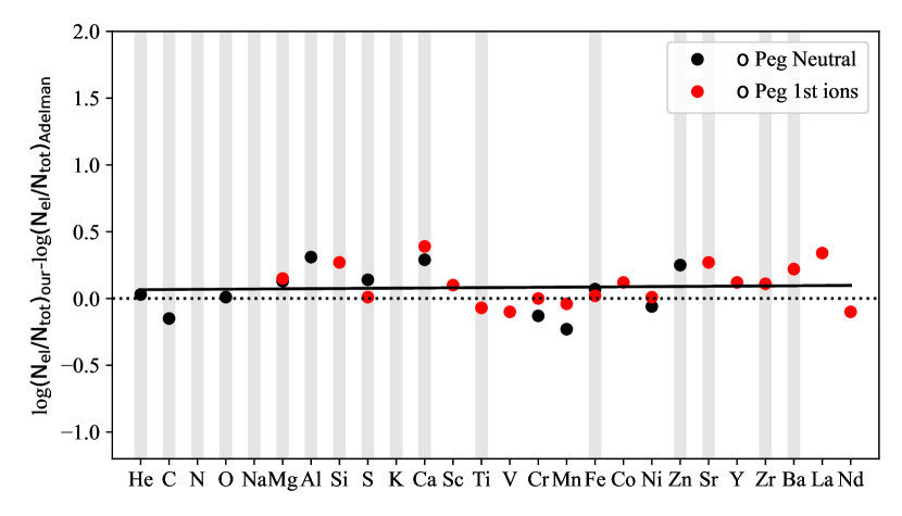
Figure 3: The difference of abundances derived in this study and those from Adelman et al. (2015a) for $o$ PegL̇inear regression is shown by the solid line. Shaded stripes indicate chemical elements, for which we determine abundances in NLTE.

The differences between our results and the literature data are partially caused by taking into account NLTE effects. Using different stellar atmosphere parameters and different transition probabilities also contributes to the discrepancy. While the average abundance difference of $\sim$0.1 dex does not exceed the abundance uncertainties, it is worth noting that, for individual elements, the abundance difference reaches $\sim$0.3 dex, as in the case of calcium in $o$ Peg.

Table 5: Average abundances in the comparison stars Sirius, HD 72660, 21 Peg and HD 32115.

Ion	Sirius		HD 72660		21 Peg		HD 32115		Refs.
	$\log\varepsilon$	[X/H]	$\log\varepsilon$	[X/H]	$\log\varepsilon$	[X/H]	$\log\varepsilon$	[X/H]
He*	10.82(03)	-0.10	10.72(04)	-0.20	10.90(02)	-0.02			(1)
C*	7.71(14)	-0.76	8.02(08)	-0.45	8.38(09)	-0.09	8.45(08)	-0.02	(2)
N*	7.75(07)	-0.10	7.32(08)	-0.53	7.53(07)	-0.32	7.96(01)	0.11	(4)
O*	8.44(05)	-0.29	8.43(07)	-0.30	8.63(02)	-0.10	8.86(11)	0.13	(2)
Na*	6.54(02)	0.27	6.66(02)	0.39	6.24(01)	-0.03	6.17(07)	-0.10	(2)
Mg*	7.51(06)	-0.01	7.77(06)	0.25	7.50(04)	-0.02	7.58(06)	0.06	(2)
Al*	6.34(01)	-0.08	6.98(08)	0.56	6.29(04)	-0.13	6.25(11)	-0.17	(4)
Si*	7.72(11)	0.21	7.83(09)	0.32	7.50(13)	-0.01	7.59(15)	0.08	(2)
S i*	7.59(12)	0.44			7.46(05)	0.31	7.22(06)	0.07	(4)
S ii	7.53(20)	0.38	7.37(12)	0.22	7.24(14)	0.09			(4)
K*			5.34(20)	0.27			5.00(20)	-0.07	(4)
Ca*	6.09(05)	-0.18	6.62(09)	0.35	6.30(15)	0.03	6.39(09)	0.12	(2)
Sc	1.99(11)	-1.05	2.63(05)	-0.41	2.60(06)	-0.44	3.22(10)	0.18	(2)
Ti*	5.15(04)	0.25	5.45(08)	0.55	4.80(04)	-0.10	4.76(05)	-0.14	(2)
V	4.50(04)	0.55	4.64(06)	0.69	3.93(07)	-0.02	3.93(11)	-0.02	(4)
Cr	6.24(08)	0.61	6.17(11)	0.54	5.61(06)	-0.02	5.77(12)	0.14	(4)
Mn	5.76(01)	0.29	5.86(08)	0.39	5.42(13)	-0.05	5.30(15)	-0.17	(4)
Fe*	7.98(06)	0.53	8.10(16)	0.65	7.51(07)	0.06	7.55(11)	0.10	(2)
Co	5.73(20)	0.87	5.78(07)	0.92	5.07(07)	0.21	4.70(04)	-0.16	(4)
Ni	6.91(07)	0.72	7.01(07)	0.81	6.32(08)	0.12	6.07(09)	-0.13	(4)
Zn*	5.58(02)	0.97	5.61(04)	1.00	4.98(20)	0.37	4.34(01)	-0.27	(3)
Sr*	3.83(04)	0.95	4.35(04)	1.47	3.49(02)	0.61	3.28(04)	0.40	(2)
Y*	3.37(08)	1.22	3.52(03)	1.37	2.92(14)	0.77	2.28(11)	0.13	(4)
Zr*	3.40(13)	0.85	3.85(11)	1.30	2.92(10)	0.37	2.82(03)	0.27	(2)
Ba*	3.74(06)	1.57	3.67(03)	1.50	3.16(05)	0.99	2.47(07)	0.30	(2)
Nd	2.94(03)	1.52	2.74(04)	1.32	1.96(01)	0.54	1.31(01)	-0.12	(2)
$T_{\rm eff}$	9850		9700		10400		7250		(2)
$\log{g}$	4.30		4.10		3.55		4.20		(2)

Note. Elements with NLTE abundance determinations are marked by *. The standard deviation is given in parentheses. Abundances taken from our earlier studies are shown by boldface. References are (1) – Korotin & Ryabchikova (2018); (2) – Mashonkina et al. (2020); (3) – Sitnova et al. (2022); (4) – this study.

The derived abundances for the sample stars and the comparison stars are shown in Fig. 4. We split stars in two groups: normal A stars ($\gamma$ Gem, $o$ Peg, 21 Peg, and HD 32115, Fig. 4(a)) and Am stars ($o$ Peg, $\theta$ Vir, Sirius, and HD 72660, Fig. 4(b)). NLTE results are displayed in the top panels, while pure LTE abundances are displayed in the bottom panels (Fig. 4(c), Fig. 4(d)). For each group of stars, NLTE leads to smaller abundance differences between different stars. This effect is the most pronounced for light elements.

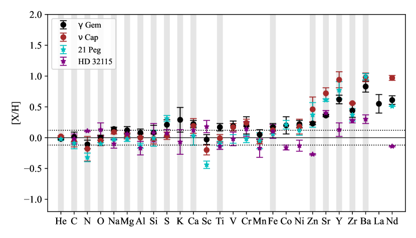
(a)

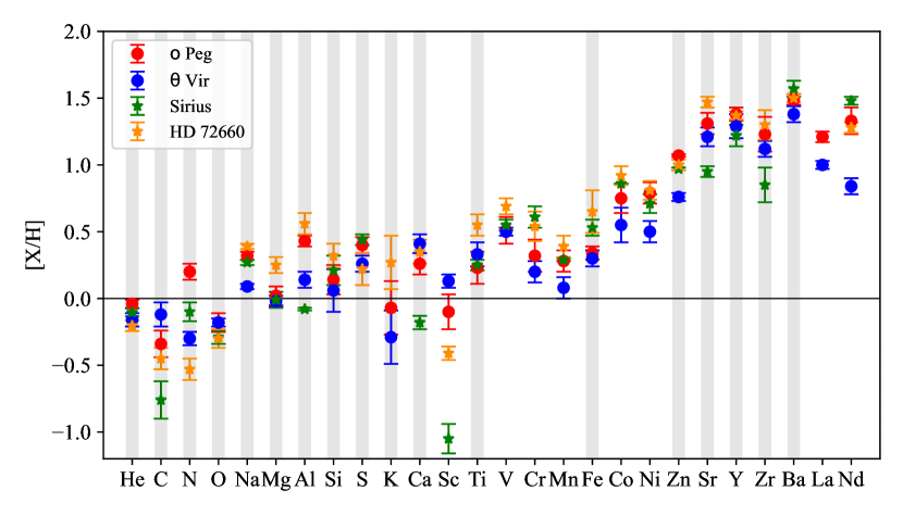
(b)

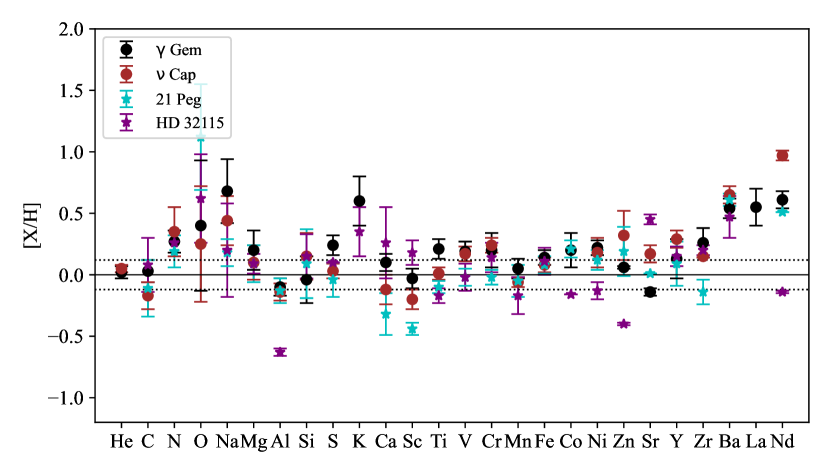
(c)

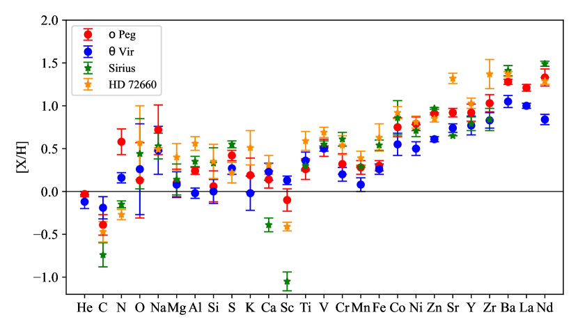
(d)

Figure 4: Sample stars abundances in comparison with the abundances in normal stars HD 32115 and 21 Peg (a) and Am stars Sirius and HD 72660 (b). The dotted lines indicate 3$\sigma$ ($\pm$0.12 dex) abundance error, which is typical for solar abundance analysis. Shaded stripes indicate chemical elements, for which we determine abundances in NLTE. Bottom panels (c) and (d) show LTE results for the same stars.

5.1 Normal stars

A star can be considered normal if its abundances for elements from He to Ni match solar values, with differences within $\pm$0.15 dex. Our detailed NLTE analysis supports the classification of both $\gamma$ Gem  and $\nu$ Cap  as normal (superficially normal) stars. In $\gamma$ Gem and $\nu$ Cap, abundances of all elements up to Fe, except for N and Sc, agree within $\pm$0.12 dex with the abundances in HD 32115 and 21 Peg, which are classified as normal stars. Nitrogen deficiency in $\nu$ Cap  and in 21 Peg may be due to an overestimation of the NLTE effects. Scandium abundance was derived using Sc ii lines, and abundance diversity may be caused by neglecting the NLTE effects. The NLTE abundance corrections for Sc ii lines were discussed in Mashonkina et al. (2020). They are expected to be positive for our sample stars.

The elements heavier than Zn show overabundances of up to 1 dex. The possible correlation between the neutron capture elements (Sr-Zr-Ba-Nd) excess and effective temperature was noticed in Paper  i. Here we refine this guess with the larger number of normal stars. The effective temperatures of our four normal sharp-lined stars range from 7200 to 10400 K. To extend this range towards higher $T_{\rm eff}$, we included Sr abunndance in the normal B-type star $\pi$ Cet ($T_{\rm eff}$ = 12800 K) from Paper  i. No lines of other heavy elements were detected in this star.

Fig. 5 shows an excess of heavy elements Zn-Ba-Sr-Y-Zr as a function of the effective temperature. A gradual increase in [X/H] of up to +1 dex is observed as $T_{\rm eff}$ increases from 7200 to 10000 K. With a further increase in $T_{\rm eff}$, a hint of a decreasing trend can be noticed, and the Sr excess mostly reaches zero (solar abundance) at $T_{\rm eff}$ = 12800 K. To support our present result, abundance studies of more stars with slow rotation and solar metallicity in temperature ranges 8000–9000 K and 9500-12000 K are required.

We estimated $T_{\rm eff}$ = 12000 K as an upper limit for detection of the resonance Ba ii 4554 Å line in a spectrum of a star with $v\sin{i}$ = 25 km s^-1 and Ba excess of +1 dex. The task becomes more difficult taking into account the fact that the mean projected rotational velocity of A and B-type stars exceeds 50 km s^-1. There is at least one star 134 Tau with $v\sin{i}$ = 27 km s^-1 and $T_{\rm eff}$ = 10825 K (Adelman, 1991), which was classified as a normal solar abundance star. We have extracted a spectrum of 134 Tau from the HARPS spectrograph archive, examined it and found that spectral lines shape provides a strong evidence for 134 Tau being a fast rotator seen pole-on similar to Vega. This is demonstrated in Fig. 6 where the spectrum of 134 Tau is compared with the Vega spectrum. More sophisticated methods are required for spectrum and abundance analysis that is beyond the scope of our paper. However, we estimated Sr and Ba abundances in 134 Tau based on the equivalent widths of Sr ii 4077, 4215 Å and Ba ii 4554 Å lines and using stellar parameters from (Adelman, 1991). Sr and Ba abundances are plotted in Fig. 5 by the open symbols. These results support the decreasing trend for the Sr and Ba excess in normal stars with $T_{\rm eff}$ $>$ 10000 K.

5.2 Am stars

A comparison of the abundance patterns of $o$ Peg  and $\theta$ Vir  and known Am stars Sirius and HD 72660 is shown in Fig. 4(b). $o$ Peg  and $\theta$ Vir  show abundance patterns partially similar to hot representatives of mild Am stars: close to solar/small underabundance of light elements, and then a gradual increase of up to 1.5 dex in [X/H] towards Nd. Our sample of Am stars including the comparison stars has a narrow effective temperature range around 9700$\pm$150 K, and this results in close abundances for most elements. However, for the number of elements (C, N, K, Ca, Sc) the large abundance dispersion exceeding 0.5 dex is found, and it cannot be explained by the temperature effect.

CNO elements are moderately underabundant, but while O deficiency is practically the same, $\approx-0.25$ dex in our Am stars, C and N abundance dispersion reaches 0.7 dex. Potassium abundance is measured in three stars of our sample, and it spreads over $\pm$0.3 dex around the solar value. For Sirius, we estimated an upper limit for the potassium abundance by analysing an extremely weak K i 7698.96 Å line. The estimated abundance was found to be close to the solar value and comparable to that observed in $o$ Peg.

While the classical Am-star classification criteria (Ca and, to a greater extent, Sc abundance deficiency) are evident in Sirius, they are nearly absent in $o$ Peg and $\theta$ Vir. The expected positive NLTE abundance corrections for Sc may remove completely small Sc deficiency in $o$ Peg. The NLTE analysis of Sc ii lines in A type stars is urgently needed because Sc deficiency is considered as one of the classification characteristics of Am-stars. The difference between Ca and Sc abundances in Sirius and those observed in $o$ Peg and $\theta$ Vir cannot be explained by a temperature effect because three stars have close temperatures. Obviously, classification characteristics of Am stars require more careful analysis based on detailed NLTE abundance analysis of a large sample of stars with small/moderate rotational velocities.

Nothing can be said about the temperature dependence of the neutron capture elements in our sample of Am stars because all four objects studied have similar effective temperatures. We may only conclude that both in normal and Am stars Ba has the largest abundance excess compared to nearby neutron capture elements such as Sr-Y-Zr and Nd.

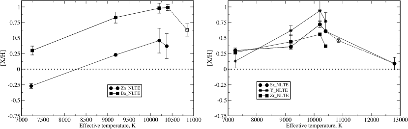
Figure 5: Neutron capture element abundance ratios in normal A stars as a function of $T_{\rm eff}$. Abundance ratios in 134 Tau are shown by the open symbols.

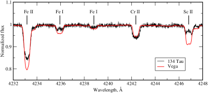
Figure 6: Comparison of the observed spectra of 134 Tau (black line) and Vega (red line).

6 Evolutionary status

We estimated the evolutionary status of our stars putting their $\log{g}$ and $T_{\rm eff}$ on the isochrones extracted from the single-star MESA (Modules for Experiments in Stellar Astrophysics, Choi et al., 2016) theoretical stellar evolution model grid computed with the solar-scaled abundance ratios (see Fig. 7). MESA has two variants for accounting for stellar rotation: V(initial)/V(critical)=0 and V(initial)/V(critical)=0.4. Our sample stars are slowly rotating objects so we use the first value. While, our stars has different abundance patterns, their average metallicities (z-values) do not differ significantly from the solar value. Therefore, we adopted MESA isochrones calculated with the solar metallicity. Three Am stars that have similar abundance patterns are sitting on the same isochrone with an age of $\log{t}$ = 8.6 ($t\approx$400 Myr), while another Am star Sirius is younger, $t\approx$230 Myr.

The best way to explore evolutionary effects in creation of abundance anomalies is to study groups of slow rotating A-B stars in open clusters of different ages. According to the results by Casamiquela et al. (2022) who compared averaged abundance patterns of Am stars in four open clusters in age interval 100–700 Myr, abundances of 11 elements from O to Ba are consistent from cluster to cluster.

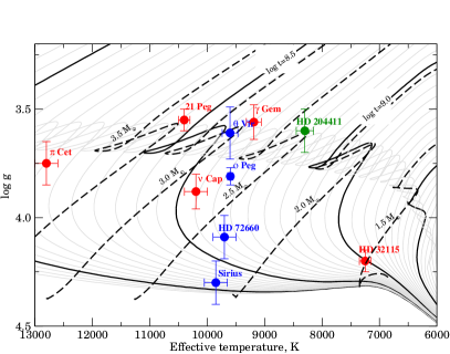
Figure 7: Position of the normal stars (red filled circles) and Am stars (blue filled circles) on the MESA isochrones (solid thick and thin lines) calculated with the solar metallicity. Evolutionary tracks are shown by dashed lines. Green filled circle indicates the position of the Ap star HD 204411.

7 Comparison of A, Am, and Ap-type stars

As we mention in the Introduction, the origin of the chemical anomalies is attributed to the atomic diffusion processes. These processes are slow, therefore a relatively stable atmosphere is necessary to support the element separation. Rapid rotation as well as turbulent motions will destroy any element separation homogenising atmospheric abundances. In principle, two slowly rotating stars with similar ages and atmospheric parameters should demonstrate similar atmospheric abundance distribution. However, it is well-known in the literature that there are A-type stars of various types exhibiting diverse abundance anomalies. The existence of different types of A stars suggests that diffusion is not the only mechanism responsible for abundance peculiarities. At least, in magnetic chemically peculiar (Ap) stars, diffusion is considered to be the primary cause of abundance anomalies.

To estimate the contribution of diffusion to abundance patterns of A and Am sample stars, we included for comparison Ap star HD 204411 with $T_{\rm eff}$ = 8300 K, $\log{g}$ = 3.6 (Romanovskaya et al., 2019), and a weak averaged surface magnetic field modulus $\langle B_{\rm s}\rangle$$\leq$0.8 kG, which has only a minor effect on abundances. Similar to $\gamma$ Gem  HD 204411 is approaching the end of its main sequence life (Fig. 7). $\gamma$ Gem  and $\theta$ Vir  are selected as representatives of A and Am stars, respectively. Additionally, HD 72660 is included as an Am star with a different mass.

For comparison of the abundance pattern in different stars we adopt $\gamma$ Gem as the reference star. To achieve more precise matching, we calculate line-by-line differential abundances with respect to $\gamma$ Gem for the selected stars. For Ap star HD 204411, we took LTE abundances from Romanovskaya et al. (2019) and applied the NLTE abundance corrections for C, O, Na, Mg, Si, Ca, Zn, Sr, Y, Zr, Ba. Fig. 8 shows abundance difference between the Am stars $\theta$ Vir and HD 72660, and Ap star HD 204411 relative to the normal star $\gamma$ Gem.

In Ap star HD 204411, atomic diffusion produces the observed stratification of Ca, Cr, Fe (Romanovskaya et al., 2019), and it also appeared as the violation of the ionisation balance (Fig. 8): there is a significant difference in abundances from the lines of neutral species and the first ions of the same chemical element. In contrast to HD 204411, the ionisation balance is fulfilled in our A and Am stars.

All neutron capture elements except Sr have lower abundances in Ap star HD 204411 compared to the normal A star, and it is Sr, not Ba that has the largest abundance among elements Zn-Sr-Y-Zr-Ba. It should be noted that in Ap stars with strong magnetic fields of  4 kG, an excess of neutron capture elements of about 2 dex is observed, with barium showing the lowest abundance among all neighbouring elements (see Fig. 1.6a in Romanovskaya, 2022).

Abundances of Fe-peak element, excluding Cr, in Ap star are close to that in Am star HD 72660. Cr is the most abundant among Fe-peak elements and its overabundance together with Sr is one of the classification criterium of Ap stars (SrCr stars).

But what defines a difference between normal A and Am star? It is possible that in Am stars the chemical composition is affected by the presence of a secondary component: Sirius has a white dwarf companion; HD 72660 is a suspected single-line spectroscopic binary (Royer et al., 2014), $o$ Peg  and $\theta$ Vir  are double or multiple stars (see Section 2.1 for details). The binarity of HD 72660 was confirmed by the observed proper motion anomaly (Kervella et al., 2019). However, a normal star $\gamma$ Gem is also a spectroscopic binary. Although the fast rotation should prevent atomic diffusion process, however if 134 Tau is confirmed to be normal pole-on fast rotating A star, then Sr and Ba overabundances is difficult to explain by this mechanism.

During the comparison analysis, the following questions arise:
$\bullet$ what distinguishes normal A type stars from Am stars?
$\bullet$ which mechanisms are responsible for abundance diversity among A type stars with close fundamental parameters?
$\bullet$ do all A stars have non-solar abundances of neutron capture elements?
$\bullet$ are there normal A type stars with solar abundances?

The first two questions can be addressed by theoretical studies of stellar evolution and modelling of processes in A-type stars, which lie beyond the scope of this study. Here we aim to provide as accurate as possible observational constraints using a careful stellar parameter determination and state of the art spectroscopic analysis. We present our comments regarding the possible impact of a secondary component on Am-type stars phenomenon.

The latter questions are attributed to our findings concerning the excess of heavy elements and its correlation with the effective temperature. In this study, we confirm the hypothesis proposed in Paper  i, which suggests that the excess of heavy elements in A-type stars increases with $T_{\rm eff}$. In addition to these conclusion, here we found that the heavy element excess reaches its maximum at $T_{\rm eff}$ = 10000 K, and as $T_{\rm eff}$ increases further, the element excess gradually decreases until it reaches the solar value at $T_{\rm eff}$ = 13000 K. This indicates that stars with solar element abundances can be found among late B-type stars with $T_{\rm eff}$ > 13000 K.

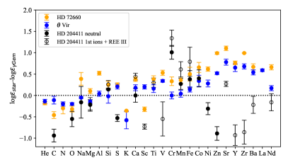
Figure 8: Differential abundances in Am stars HD 72660, $\theta$ Vir and Ap star HD 204411 relative to $\gamma$ Gem.

8 Conclusions

We present a self-consistent abundance analysis for elements from He to Nd in slowly rotating normal A and metallic line Am stars in temperature range 9200–10200 K. We refined their fundamental parameters with the SME package, spectral energy distribution, and the hydrogen line profiles. We analysed the chemical abundances of 26 elements, for 18 of them the analysis was performed with NLTE approach.

Our abundance analysis supports the classification of $\gamma$ Gem and $\nu$ Cap as normal A stars with enhanced neutron capture element abundances and $o$ Peg and $\theta$ Vir as Am stars. We found that, in NLTE, the abundance difference between stars of the same type reduces.

For normal A-type sample stars, abundances of elements from He to Ni are close to solar values, while elements heavier than Zn are overabundant with Ba showing the largest excess. We confirm a gradual rise of the heavy element (Zn, Sr, Y, Zr, Ba) abundance excess up to +1 dex with $T_{\rm eff}$ increasing from 7200 to 10000 K noted first in Paper  i. We found that with a further increase in $T_{\rm eff}$, a decreasing trend can be noticed, and the Sr excess mostly reaches zero (solar abundance) at $T_{\rm eff}$ = 12800 K. To support our present result, abundance studies of more stars with slow rotation and solar metallicity in temperature ranges 8000–9000 K and 9500–12000 K are required.

For metallic line Am stars of our sample, abundance patterns are similar to hot representatives of mild Am stars: close to solar/small underabundance of light elements, and then a gradual increase of up to 1.5 dex in [X/H] towards Nd. Our sample stars do not show Ca-Sc deficiency that is pronounced in Sirius. In contrast, a small Ca excess is observed in $o$ Peg, $\theta$ Vir, and HD 72660. The expected positive NLTE abundance corrections for Sc may remove completely a small Sc deficiency in $o$ Peg, and, perhaps, in HD 72660. Therefore, the classification criteria of Am stars based on significant Ca and Sc deficiency cannot be applied. A comprehensive NLTE abundance analysis of a substantial stellar sample is necessary to reevaluate the classification criteria of Am stars.

Comparison of the atmospheric abundances in the representatives of different types of A stars (normal, Am and Ap) with similar fundamental parameters showed a diversity in the abundance patterns that cannot be explained by a simple atomic diffusion process.

Data Availability

Spectra of program stars normalised to the continuum level are provided as supplementary material in the form of an ASCII file in CDS. The full table of used lines with log $gf$, excitation potentials of lower level $E_{i}$, LTE and non-LTE abundances and references for oscillator strengths and hyperfine constants is available online in CDS.

Appendix A Spectral energy distributions figures

This section presents the spectral energy distributions for the stars $o$ Peg, $\theta$ Vir, $\nu$ Cap. See details in section 3.

Figure 9: Spectral energy distribution of $o$ Peg  in the UV, visual and IR spectral regions. Black solid line shows theoretical SED  calculation with the model atmosphere parameters t9552g38. IUE and TD1 points were raised by a factor of 1.05.

References

- Adelman (1991) Adelman S. J., 1991, MNRAS, 252, 116
- Adelman et al. (1989) Adelman S. J., Pyper D. M., Shore S. N., White R. E., Warren Jr. W. H., 1989, A&AS, 81, 221
- Adelman et al. (2002) Adelman S. J., Pintado O. I., Nieva M. F., Rayle K. E., Sanders S. E. J., 2002, A&A, 392, 1031
- Adelman et al. (2015a) Adelman S. J., Gulliver A. F., Heaton R. J., 2015a, PASP, 127, 58
- Adelman et al. (2015b) Adelman S. J., Gulliver A. F., Kaewkornmaung P., 2015b, PASP, 127, 340
- Alecian (1996) Alecian G., 1996, A&A, 310, 872
- Amarsi & Barklem (2019) Amarsi A. M., Barklem P. S., 2019, A&A, 625, A78
- Andrievsky et al. (2021) Andrievsky S. M., Korotin S. A., Kovtyukh V. V., Khrapaty S. V., Rudyak Y., 2021, Astronomische Nachrichten, 342, 887
- Becker et al. (1981) Becker W., Blatt R., Werth G., 1981, in Precision Measurement and Fundamental Constants. p. 99
- Blatt & Werth (1982) Blatt R., Werth G., 1982, Phys. Rev. A, 25, 1476
- Blazère et al. (2020) Blazère A., Petit P., Neiner C., Folsom C., Kochukhov O., Mathis S., Deal M., Landstreet J., 2020, MNRAS, 492, 5794
- Butler (1984) Butler K., 1984, Ph.D. Thesis, University of London
- Caffau et al. (2019) Caffau E., et al., 2019, A&A, 628, A46
- Carlsson (1986) Carlsson M., 1986, Uppsala Astronomical Observatory Reports, 33
- Casamiquela et al. (2022) Casamiquela L., Gebran M., Agüeros M. A., Bouy H., Soubiran C., 2022, AJ, 164, 255
- Castelli & Kurucz (2003) Castelli F., Kurucz R. L., 2003, in Piskunov N., Weiss W. W., Gray D. F., eds, Vol. 210, Modelling of Stellar Atmospheres. p. A20 (arXiv:astro-ph/0405087), doi:10.48550/arXiv.astro-ph/0405087
- Cenarro et al. (2007) Cenarro A. J., et al., 2007, MNRAS, 374, 664
- Choi et al. (2016) Choi J., Dotter A., Conroy C., Cantiello M., Paxton B., Johnson B. D., 2016, ApJ, 823, 102
- Cohen et al. (2003) Cohen M., Wheaton W. A., Megeath S. T., 2003, AJ, 126, 1090
- Cutri et al. (2003) Cutri R. M., et al., 2003, VizieR Online Data Catalog, 2246
- Di Benedetto (1998) Di Benedetto G. P., 1998, A&A, 339, 858
- Dobrichev et al. (1987) Dobrichev V. M., Riabchikova T. A., Raikova D. V., 1987, Astrofizika, 26, 55
- Erspamer & North (2003) Erspamer D., North P., 2003, A&A, 398, 1121
- Fekel (1999) Fekel F. C., 1999, in Hearnshaw J. B., Scarfe C. D., eds, Astronomical Society of the Pacific Conference Series Vol. 185, IAU Colloq. 170: Precise Stellar Radial Velocities. p. 378
- Fekel & Tomkin (1993) Fekel F. C., Tomkin J., 1993, AJ, 106, 1156
- Fitzpatrick (1999) Fitzpatrick E. L., 1999, PASP, 111, 63
- Gaia Collaboration (2020) Gaia Collaboration 2020, VizieR Online Data Catalog, p. I/350
- Giddings (1981) Giddings J., 1981, Ph.D. Thesis, University of London
- Gray et al. (2003) Gray R. O., Corbally C. J., Garrison R. F., McFadden M. T., Robinson P. E., 2003, AJ, 126, 2048
- Hill & Landstreet (1993) Hill G. M., Landstreet J. D., 1993, A&A, 276, 142
- Irimia & Fischer (2005) Irimia A., Fischer C. F., 2005, Physica Scripta, 71, 172
- Kervella et al. (2019) Kervella P., Arenou F., Mignard F., Thévenin F., 2019, A&A, 623, A72
- Kochukhov (2018) Kochukhov O., 2018, BinMag: Widget for comparing stellar observed with theoretical spectra (ascl:1805.015)
- Koleva & Vazdekis (2012) Koleva M., Vazdekis A., 2012, A&A, 538, A143
- Korotin (2009) Korotin S. A., 2009, Astronomy Reports, 53, 651
- Korotin & Ryabchikova (2018) Korotin S. A., Ryabchikova T. A., 2018, Astronomy Letters, 44, 621
- Korotin et al. (1999) Korotin S. A., Andrievsky S. M., Luck R. E., 1999, A&A, 351, 168
- Kramida et al. (2022) Kramida A., Yu. Ralchenko Reader J., and NIST ASD Team 2022, NIST Atomic Spectra Database (ver. 5.10), [Online]. Available: https://physics.nist.gov/asd [2022, December 18]. National Institute of Standards and Technology, Gaithersburg, MD.
- Lallement et al. (2014) Lallement R., Vergely J. L., Valette B., Puspitarini L., Eyer L., Casagrande L., 2014, A&A, 561, A91
- Liu et al. (2011) Liu Y. P., Gao C., Zeng J. L., Shi J. R., 2011, A&A, 536, A51
- Lodders (2021) Lodders K., 2021, Space Sci. Rev., 217, 44
- Lyubimkov et al. (2011) Lyubimkov L. S., Lambert D. L., Korotin S. A., Poklad D. B., Rachkovskaya T. M., Rostopchin S. I., 2011, MNRAS, 410, 1774
- Mashonkina et al. (2020) Mashonkina L., Ryabchikova T., Alexeeva S., Sitnova T., Zatsarinny O., 2020, MNRAS, 499, 3706
- Mason et al. (2001) Mason B. D., Wycoff G. L., Hartkopf W. I., Douglass G. G., Worley C. E., 2001, AJ, 122, 3466
- McAlister & Hendry (1982) McAlister H. A., Hendry E. M., 1982, ApJS, 48, 273
- Michaud (1970) Michaud G., 1970, ApJ, 160, 641
- Michaud (1982) Michaud G., 1982, ApJ, 258, 349
- Miles & Wiese (1969) Miles B. M., Wiese W. L., 1969, Atomic Data, 1, 1
- Monier et al. (2018) Monier R., Gebran M., Royer F., Kilicoglu T., Frémat Y., 2018, ApJ, 854, 50
- Neretina et al. (2020) Neretina M. D., Mashonkina L. I., Sitnova T. M., Yakovleva S. A., Belyaev A. K., 2020, Astronomy Letters, 46, 621
- Piskunov & Valenti (2017) Piskunov N., Valenti J. A., 2017, A&A, 597, A16
- Preston (1974) Preston G. W., 1974, ARA&A, 12, 257
- Prugniel et al. (2011) Prugniel P., Vauglin I., Koleva M., 2011, A&A, 531, A165
- Przybilla et al. (2011) Przybilla N., Nieva M.-F., Butler K., 2011, Journal of Physics Conference Series, 328, 012015
- Richer et al. (2000) Richer J., Michaud G., Turcotte S., 2000, ApJ, 529, 338
- Romanovskaya (2022) Romanovskaya A. M., 2022, PhD thesis, Institute of astronomy RAS
- Romanovskaya et al. (2019) Romanovskaya A., Ryabchikova T., Shulyak D., Perraut K., Valyavin G., Burlakova T., Galazutdinov G., 2019, MNRAS, 488, 2343
- Romanovskaya et al. (2020) Romanovskaya A. M., Ryabchikova T. A., Shulyak D. V., 2020, INASAN Science Reports, 5, 219
- Royer et al. (2014) Royer F., et al., 2014, A&A, 562, A84
- Rubin et al. (2022) Rubin D., et al., 2022, ApJS, 263, 1
- Ryabchikova et al. (2016) Ryabchikova T., et al., 2016, MNRAS, 456, 1221
- Schwarz et al. (2009) Schwarz R., Süli Á., Dvorak R., 2009, MNRAS, 398, 2085
- Seaton (1962) Seaton M. J., 1962, in Bates D. R., ed., Atomic and Molecular Processes. p. 375
- Shorlin et al. (2002) Shorlin S. L. S., Wade G. A., Donati J. F., Landstreet J. D., Petit P., Sigut T. A. A., Strasser S., 2002, A&A, 392, 637
- Shulyak et al. (2004) Shulyak D., Tsymbal V., Ryabchikova T., Stütz C., Weiss W. W., 2004, A&A, 428, 993
- Sitnova et al. (2022) Sitnova T. M., Yakovleva S. A., Belyaev A. K., Mashonkina L. I., 2022, MNRAS, 515, 1510
- Takeda et al. (2018) Takeda Y., Kawanomoto S., Ohishi N., Kang D.-I., Lee B.-C., Kim K.-M., Han I., 2018, PASJ, 70, 91
- Thalmann et al. (2014) Thalmann C., et al., 2014, A&A, 572, A91
- Thompson et al. (1978) Thompson G. I., Nandy K., Jamar C., Monfils A., Houziaux L., Carnochan D. J., Wilson R., 1978, Catalogue of stellar ultraviolet fluxes. A compilation of absolute stellar fluxes measured by the Sky Survey Telescope (S2/68) aboard the ESRO satellite TD-1. The Science Research Council, U.K.
- Tsymbal et al. (2019) Tsymbal V., Ryabchikova T., Sitnova T., 2019, in Kudryavtsev D. O., Romanyuk I. I., Yakunin I. A., eds, Astronomical Society of the Pacific Conference Series Vol. 518, Physics of Magnetic Stars. pp 247–252
- Valenti & Piskunov (1996) Valenti J. A., Piskunov N., 1996, A&AS, 118, 595
- Van Hove et al. (1982) Van Hove M., Borghs G., DeBisschop P., Silverans R. E., 1982, Journal of Physics B Atomic Molecular Physics, 15, 1805
- Villemoes et al. (1993) Villemoes P., Arnesen A., Heijkenskjold F., Wannstrom A., 1993, Journal of Physics B Atomic Molecular Physics, 26, 4289
- Watson (1971) Watson W. D., 1971, A&A, 13, 263
- Wehrhahn et al. (2023) Wehrhahn A., Piskunov N., Ryabchikova T., 2023, A&A, 671, A171
- Wendt et al. (1984) Wendt K., Ahmad S. A., Buchinger F., Mueller A. C., Neugart R., Otten E. W., 1984, Zeitschrift fur Physik A Hadrons and Nuclei, 318, 125
- Wiese et al. (1966) Wiese W. L., Smith M. W., Glennon B. M., 1966, Atomic transition probabilities. Vol.: Hydrogen through Neon. A critical data compilation
- Woolley & Allen (1948) Woolley R. D. V. R., Allen C. W., 1948, MNRAS, 108, 292
- Zatsarinny & Bartschat (2005) Zatsarinny O., Bartschat K., 2005, Phys. Rev. A, 71, 022716
- Zatsarinny & Bartschat (2006) Zatsarinny O., Bartschat K., 2006, J. Phys. B, 39, 2861
- Zorec et al. (2009) Zorec J., Cidale L., Arias M. L., Frémat Y., Muratore M. F., Torres A. F., Martayan C., 2009, A&A, 501, 297
- ten Brummelaar et al. (2000) ten Brummelaar T., Mason B. D., McAlister H. A., Roberts Lewis C. J., Turner N. H., Hartkopf W. I., Bagnuolo William G. J., 2000, AJ, 119, 2403
- van Hove et al. (1985) van Hove M., Borghs G., de Bisschop P., Silverans R. E., 1985, Zeitschrift fur Physik A Hadrons and Nuclei, 321, 215
- van Leeuwen (2007) van Leeuwen F., 2007, A&A, 474, 653
- van Regemorter (1962) van Regemorter H., 1962, ApJ, 136, 906