Boosting Fair Classifier Generalization through Adaptive Priority Reweighing

Abstract.

With the increasing penetration of machine learning applications in critical decision-making areas, calls for algorithmic fairness are more prominent. Although there have been various modalities to improve algorithmic fairness through learning with fairness constraints, their performance does not generalize well in the test set. A performance-promising fair algorithm with better generalizability is needed. This paper proposes a novel adaptive reweighing method to eliminate the impact of the distribution shifts between training and test data on model generalizability. Most previous reweighing methods propose to assign a unified weight for each (sub)group. Rather, our method granularly models the distance from the sample predictions to the decision boundary. Our adaptive reweighing method prioritizes samples closer to the decision boundary and assigns a higher weight to improve the generalizability of fair classifiers. Extensive experiments are performed to validate the generalizability of our adaptive priority reweighing method for accuracy and fairness measures (i.e., equal opportunity, equalized odds, and demographic parity) in tabular benchmarks. We also highlight the performance of our method in improving the fairness of language and vision models. The code is available at https://github.com/che2198/APW.

1. Introduction

With the increasing penetration of machine learning applications in critical decision-making areas, such as mortgage approval (Madras et al., 2018), employee selection (Pessach and Shmueli, 2023), recidivism prediction (Beutel et al., 2019), and healthcare, calls for algorithmic fairness are more prominent. In reality, machine learning tools can behave in unintentional or even harmful ways (Wan et al., 2023). For example, research on the COMPAS dataset (Chouldechova, 2017) shows that a well-calibrated classification algorithm tends to classify African-American defendants with a higher risk of re-conviction while classifying white defendants with lower risk (Angwin et al., 2022). In this case, the machine learning algorithms perpetuated and amplified the long-standing discrimination against people of color (Wang et al., 2019). Both categorizations produced during data collection and/or analysis and the data itself are persistent, which paves the way for algorithms to compound the impact of historically biased data. More importantly, bias exists in forms of distribution, thus almost impossible to address bias by discarding individual instances. Therefore, it is much more difficult to achieve fairness by removing sensitive attributes from the data. Machine learning researchers have been focusing on higher classification accuracy, yet our study suggests the need to shift away from the fixation on accuracy and be actively attentive to mitigating biases from training data and ensuring generalizable performance across real-world datasets.

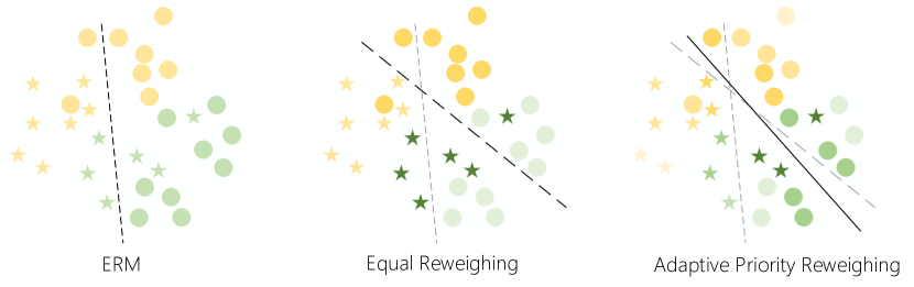
Figure 1. Illustration of our adaptive priority reweighing method. Samples of different shapes indicate samples with different labels, different colors refer to different sensitive attributes, and darker color indicates higher weight. In ERM, fairness is disregarded altogether; all samples have the same weight, which could easily lead to unfairness. In equal reweighing, (sub)groups are created and all points within one (sub)group are assigned the same weight, ensuring improved fairness on the training set. However, using equal reweighing methods induces many points clustered around the decision boundary, which limits the generalization of fair classifiers. In comparison, our method models the distance from the sample to the decision boundary, which improves the generalizability of fair classifiers.

In the recent decade, machine learning researchers have engaged in the conversation of algorithmic fairness by investigating the correlation between model output and sensitive attributes (e.g., gender and race). Diverse fairness metrics are proposed to measure the disparities in model output between different sensitive attributes. In order to improve model performance in measuring fairness, we identify fairness as a constraint term, enabling fairness to be improved by solving the constrained optimization problem. Existing methods use various regularization terms or constraints to address the problem, ranging from covariance (Zafar et al., 2017), equalized odds (Donini et al., 2018), to Rényi correlation (Baharlouei et al., 2019). Although they provide a shared foundation for machine learning researchers to engage in the fairness conundrum, they all suffer from generalization issues. That is, although these methods minimize the value of constraints on the training set, they cannot guarantee fairness on the test set. Chuang and Mroueh (2021) (Chuang and Mroueh, 2021) and Ramachandran and Rattani (2022) (Ramachandran and Rattani, 2022) address the generalization issues of algorithmic fairness using data augmentation. Chuang and Mroueh (2021) propose applying mixup path regularization to enhance the generalizability of the fair classifier. Ramachandran and Rattani (2022) further build on the conversation by engaging with the generative model to mitigate gender classification bias. Unfortunately, both studies require training data to conform to a specific distribution, leading to a limited representation of real-world datasets and reduced accuracy.

We aim to address the generalization issue of fairness improvement, but at the same time preserve accuracy. To do that, we propose an adaptive priority weight assignment strategy to improve fairness. As illustrated in Figure 1, we first divide the subgroups using sensitive attributes and predictions of the classifier. Data points closer to the decision boundary are more likely to be wrongly classified (Kamiran and Calders, 2012) — a phenomenon highlighting the critical role of decision boundaries in a model’s generalizability (Almeida et al., 2021). Therefore, our method models the distance from data points to the decision boundary to improve the generalizability of fair classifiers. This solves the generalizability issues associated with equal reweighing. Equal reweighing methods induce the cluster of sample points around the decision boundary. Distribution shifts could cause the model to classify sample points closer to the decision boundary incorrectly, thus inducing unfairness in the test set and limiting the generalization of fair classifiers. Additionally, we take the statistical independence of model output value and sensitive attribute as the termination condition and assign higher weights to samples whose model output is closer to the decision boundary in each subgroup.

We design experiments to validate the generalizability of our adaptive priority reweighing method for accuracy and fairness measures (i.e., equal opportunity, equalized odds, and demographic parity) on tabular, language, and vision benchmarks. We further highlight the performance of our method in improving the fairness of language and vision models. Our method shows promising results in improving the fairness of any pre-trained models simply via fine-tuning. The code is available at https://github.com/che2198/APW.

We summarize our contributions as follows:

1. We propose a novel reweighing method to mitigate data bias under different fairness measures, whose performance is validated through experiments on tabular, language, and vision benchmarks.

2. Our method provides a theoretical guarantee of generalization error bound.

3. Our method improves the fairness of any pre-trained model via fine-tuning by experimenting with both language and vision benchmarks.

2. Related Work

Machine Learning Fairness. Most fairness-promoting algorithms focus on binary classification under binary-sensitive attributes. Generally, these methods can be divided into three categories: pre-processing, in-processing, and post-processing. Pre-processing methods tend to alter the sample distributions of protected variables to remove discrimination from the training data. Approaches to preprocessing data include sample selection (Roh et al., 2020b, 2021; Zhang et al., 2020), sample reweighing (Kamiran and Calders, 2012; Jiang and Nachum, 2020; Chai and Wang, 2022), fair representation learning (Zemel et al., 2013; Madras et al., 2018), fair data generation (Xu et al., 2018, 2019b; Jang et al., 2021), etc. In-processing methods incorporate changes into the objective function or impose a constraint to remove discrimination during the model training process. Fairness constraints measure the correlation between model outputs and sensitive attributes (Berk et al., 2017; Aghaei et al., 2019), such as adversarial layers (Zhang et al., 2018; Adel et al., 2019), contrastive learning loss (Zhou et al., 2021), uncorrelation constraints (Zafar et al., 2017), counterfactual logit pairing (García-Soriano and Bonchi, 2021), and mutual information (Baharlouei et al., 2019; Roh et al., 2020a). Post-processing transforms model output in different demographic groups to achieve fairness (Hardt et al., 2016; Fish et al., 2016; Woodworth et al., 2017; Pleiss et al., 2017). These methods can satisfy the fairness constraints on the training set but may not be generalized to the test set.

Recently, some methods based on data augmentation have been proposed to enhance the generalizability of fair classifiers, such as mix-up paths regularization (Chuang and Mroueh, 2021), data generation (Ramachandran and Rattani, 2022). However, these methods require training data to conform to a specific distribution or lead to computationally expensive algorithms.

Data Reweighing. The concept of data reweighing has gained considerable attention as an effective approach to improving the performance and fairness of machine learning classifiers. Various studies have explored different aspects of data reweighing techniques to address the challenges associated with biased training data and classifier fairness.

Many approaches introduced data reweighing as a means of improving classifier generalization (Chu et al., 2022; Zhou et al., 2022). They highlighted the importance of reweighing samples in the training dataset to mitigate issues arising from class imbalance, leading to improved overall classifier performance. Meanwhile, (Liu and Tao, 2015; Zhang et al., 2021) demonstrated that reweighing techniques can be instrumental in reducing bias during training, and then promoting the fairness of classifiers across diverse demographic groups.

A subset of research has concentrated specifically on fairness improvement through data reweighing. (Kamiran and Calders, 2012) pioneered the concept of fixed reweighing, which involves assigning different weights to instances from underrepresented groups to balance their influence during training. Adaptive reweighing methods, as proposed by (Krasanakis et al., 2018; Li and Liu, 2022; Wen et al., 2022; Jiang and Nachum, 2020), dynamically adjust instance weights based on the evolving characteristics of the dataset. These methods attempt to alleviate bias and enhance fairness during training.

However, these data reweighing methods on fairness minimize constraints on the training set. They cannot guarantee fairness on the test set. Unlike previous methods, we propose a novel reweighing method that addresses the generalization issue of fairness improvement and preserves classification accuracy.

3. Preliminaries

We consider the binary classification task. A sample is $z=(x,a,y)$, where $x\in\mathcal{X}$ is the input feature, $a\in\mathcal{A}=\{0,1\}$ is the sensitive attribute (e.g., gender, race, and age), and $y\in\{0,1\}$ is the prediction target. Let $Z$, $X$, $A$, and $Y$ denote the corresponding random variables of $z$, $x$, $a$, and $y$, respectively. Then, the goal of fair machine learning is to learn a binary classifier $h_{\theta}:\mathcal{X}\times\mathcal{A}\rightarrow[0,1]$ while ensuring a specific notion of fairness with respect to the sensitive attribute $A$, where $\theta$ is the parameter of the classifier. For simplicity, we denote $\hat{Y}:=f(h_{\theta}(X,A))\in\{0,1\}$ as the prediction of the classifier $h$ for variable $Z=(X,A,Y)$, where $f$ is a label function.

3.1. Group fairness

A major family of fairness concepts is the group fairness, which aims to characterize discrimination across various groups of individuals. The most used definitions of group fairness are demographic parity (Feldman et al., 2015), equalized odds (Hardt et al., 2016), and equal opportunity (Hardt et al., 2016).

Definition 0 (Fairness Definitions).

Given a data distribution $p_{z}$, a classifier $h$ satisfies:

• Demographic parity if the prediction $\hat{Y}$ is independent of the sensitive attribute $A$.

• Equalized odds if the prediction $\hat{Y}$ and the sensitive attribute $A$ are independent conditional on the target $Y$.

• Equal opportunity if $\mathbb{P}(\hat{Y}=1|A=0,Y=1)=\mathbb{P}(\hat{Y}=1|A=1,Y=1)$.

The following notions are designed to assess the degree to which the classifier satisfies the fairness constraints presented in Definition 3.1.

Definition 0 (Fairness Measures).

Given a data distribution $p_{z}$, for a binary classifier $h$:

• The demographic parity $\Delta_{\mathrm{DP}}$ is defined as:

  (1) $$\Delta_{\mathrm{DP}}(\hat{Y},p_{z})=|\mathbb{P}(\hat{Y}=1|A=0)-\mathbb{P}(\hat{Y}=1|A=1)|.$$

• The equalized odds gap $\Delta_{\mathrm{EO}}$ is defined as:

  (2) $$\Delta_{\mathrm{EO}}(\hat{Y},p_{z}) =\max_{y\in\{0,1\}}|\mathbb{P}(\hat{Y}=1|A=0,Y=y)-\mathbb{P}(\hat{Y}=1|A=1,Y=y)|.$$

• The equal opportunity gap $\Delta_{\mathrm{EOP}}$ is defined as:

  (3) $$\Delta_{\mathrm{EOP}}(\hat{Y},p_{z})=|\mathbb{P}(\hat{Y}=1|A=0,Y=1)-\mathbb{P}(\hat{Y}=1|A=1,Y=1)|.$$

Combined with Definition 3.1, it is clear that a small value of the fairness measure in Definition 3.2 would demonstrate a strong non-discriminatory of the given classifier, vice versa. When the notion $\Delta_{\mathrm{DP}}$, $\Delta_{\mathrm{EO}}$, or $\Delta_{\mathrm{EOP}}$ is equal to zero, the classifier $h$ perfectly satisfies demographic parity, equalized odds, or equal opportunity, respectively.

3.2. Subgroup weights

We divided the training samples into subgroups according to the sensitive attributes and predictions of the classifier. Specifically, we define three types of subgroups: $G_{y,a}:=\left\{\left(x_{i},a_{i},y_{i}\right):y_{i}=y,a_{i}=a\right\}$, $G_{\ast,a}:=\left\{\left(x_{i},a_{i},y_{i}\right):a_{i}=a\right\}$, and $G_{y,\ast}:=\left\{\left(x_{i},a_{i},y_{i}\right):y_{i}=y\right\}$. Let m represent the total number of training samples. We assigned the subgroup weight $W_{y,a}$ to samples that satisfy $Y=y$ and $A=a$. To quantify the number of samples within a subgroup, we introduced the notation $m_{y,a}$, defined as $m_{y,a}:=\left|\left\{i:y_{i}=y,a_{i}=a\right\}\right|$. Similarly, we defined $m_{y,\ast}:=\left|\left\{i:y_{i}=y\right\}\right|$ and $m_{\ast,a}:=\left|\left\{i:a_{i}=a\right\}\right|$. Additionally, we introduced the proportion $p_{y,a}$, which represents the fraction of samples in $G_{y,a}$ compared to the total number of samples: $p_{y,a}:=\frac{m_{y,a}}{m}$. For the equal reweighing approach, each sample is assigned a weight equal to its subgroup weight.

3.3. Generalization error

When dealing with the problem of an unknown distribution D, the empirical risk is commonly employed as an approximation of the expected risk. The empirical risk is defined as follows:

(4) $$\hat{R}_{L,D}(h)=\frac{1}{m}\sum_{i=1}^{m}L\left(y_{i},h\left(x_{i},a_{i}\right)\right),$$

where the corresponding expected risk is

(5) $$R_{L,D}(h)=R[D,h,L]=E_{(X,A,Y)\sim D}\left[\hat{R}_{L,D}(h)\right],$$

and $L$ represents a surrogate loss function, such as square loss, logistic loss, or hinge loss. The classifier is learned through the process of empirical risk minimization (ERM) (Vapnik, 1999):

(6) $$h^{\prime}=\arg\min_{h\in H}\hat{R}_{L,D}(h).$$

The consistency of $\hat{R}_{L,D}(h^{\prime})$ with respect to $\min_{h\in H}R_{L,D}(h)$ is of utmost importance when designing surrogate loss functions and learning algorithms. Let

(7) $$h^{*}=\arg\min_{h\in H}R_{L,D}(h).$$

It has been demonstrated in previous work (Anthony et al., 1999) that the following proposition holds true:

(8) $$R_{L,D}\left(h^{\prime}\right)-R_{L,D}\left(h^{*}\right)\leq 2\sup_{h\in H}\left|R_{L,D}(h)-\hat{R}_{L,D}(h)\right|.$$

The term on the right-hand side is commonly referred to as the generalization error, which measures the performance of the learned model on unseen data. The consistency of the model is ensured through the convergence of the generalization error.

4. Proposed Method

In this section, we present our Adaptive Priority Reweighing method. First, we introduce the updating rules for adaptive priority reweighing, followed by its application to prominent fairness measures, including equal opportunity, equalized odds, and demographic parity. Finally, we provide the theoretical guarantee of our method.

4.1. Updating Rules for Adaptive Priority Reweighing

For a given dataset $\{\left(x_{i},a_{i},y_{i}\right)\}_{i=1}^{m}$ of $m$ samples, the vanilla training objective without reweighing can be formulated as:

(9) $$\mathop{\min}_{\theta}\frac{1}{m}\sum_{i=1}^{m}L\left(y_{i},h_{\theta}\left(x_{i},a_{i}\right)\right).$$

Given that the unweighted training objective does not incorporate a fairness criterion, its minimizer often fails to satisfy the desired fairness requirement. To overcome this limitation, we introduce a weighting scheme for each sample to ensure the desired fairness guarantee. For example, assigning higher weights to a specific sensitive group can result in improved accuracy specifically for that group. Consequently, the batch gradient estimate provides an unbiased estimation of the reweighed empirical risk. In other words, if we draw a training example $i$ with weight $w_{i}$, the training objective can be formulated as follows:

(10) $$\mathop{\min}_{\theta}\frac{1}{m}\sum_{i=1}^{m}w_{i}L\left(y_{i},h_{\theta}\left(x_{i},a_{i}\right)\right).$$

This observation leads to the following bilevel optimization-based interpretation of how reweighing interacts with the inner optimization algorithm. Initially, batch SGD optimizes the unweighted empirical risk. Subsequently, based on the results of the inner optimization, the outer optimizer iteratively refines the weights $\boldsymbol{w}:=\left(w_{1},w_{2},\ldots,w_{m}\right)$ assigned to each training example. The inner optimizer then operates on batches drawn from a new distribution, reoptimizing the inner objective function. This process continues until convergence is achieved. Consequently, the Adaptive Priority Reweighing algorithm can be perceived as a combination of an outer optimizer and an inner optimizer, solving the following bilevel optimization problem:

(11) $$\min_{\boldsymbol{w}}\operatorname{Cost}\left(\boldsymbol{\theta}_{\boldsymbol{w}}\right),$$

(12) $$\boldsymbol{\theta}_{\boldsymbol{w}}=\underset{\boldsymbol{\theta}}{\arg\min}\frac{1}{m}\sum_{i=1}^{m}w_{i}L\left(y_{i},h_{\theta}\left(x_{i},a_{i}\right)\right),$$

where $\operatorname{Cost}\left(\cdot\right)$ captures the goal of the optimization. To simplify the discussion, we initially focus on the fairness metric $\Delta_{\mathrm{DP}}$, and then extend our analysis to include $\Delta_{\mathrm{EO}}$ and $\Delta_{\mathrm{EOP}}$. The outer optimization problem, specifically for the $\Delta_{\mathrm{DP}}$ metric, takes the following form:

(13) $$\min_{\boldsymbol{w}}|\frac{1}{m_{1,\ast}}\sum_{z_{i}\in G_{1,\ast}}f(h_{\boldsymbol{\theta}_{\boldsymbol{w}}}\left(x_{i},a_{i}\right))-\frac{1}{m_{0,\ast}}\sum_{z_{j}\in G_{0,\ast}}f(h_{\boldsymbol{\theta}_{\boldsymbol{w}}}\left(x_{j},a_{j}\right))|.$$

To address this optimization problem, we begin by computing the subgroup weight $G_{y,a}$ for each subgroup. Subsequently, we determine the sample weight based on the distance of each sample from the decision boundary within its respective subgroup. Now, let us delve into the rationale behind the calculation of the subgroup weight $G_{y,a}$.

If the classifier $h_{\theta}$ exhibits fairness, meaning that $A$ and $\hat{Y}$ are statistically independent, the expected probability $P_{\text{exp}}(\hat{Y}=1,A=1)$ can be expressed as follows:

(14) $$P_{\exp}(\hat{Y}=1,A=1):=\frac{\mid\{i:\hat{y}_{i}=1\}\mid}{m}\times\frac{\mid\{i:a_{i}=1\}\mid}{m}.$$

In reality, the observed probability is given by:

(15) $$P_{obs}(\hat{Y}=1,A=1):=\frac{\mid\{i:\hat{y}_{i}=1,a_{i}=1\}\mid}{m},$$

where $m$ represents the total number of samples. It is possible that the expected probability differs from the observed probability. If the expected probability exceeds the observed probability, it indicates a bias towards the subgroup $G_{1,1}$.

To address the bias, we aim to assign lower weights to objects that have been either deprived or favored. For this purpose, we assign weights to each subgroup $G_{y,a}$ as follows:

(16) $$W_{y,a}:=\frac{P_{\exp}(\hat{Y}=y,A=a)}{P_{obs}(\hat{Y}=y,A=a)}=\frac{\mid\{i:\hat{y}_{i}=y\}\mid\times\mid\{i:a_{i}=a\}\mid}{m\times\mid\{i:\hat{y}_{i}=y,a_{i}=a\}\mid}.$$

The weight assigned to each subgroup will be calculated as the ratio between the expected probability of observing an instance with its sensitive attribute value and prediction under the assumption of independence, and its corresponding observed probability.

Based on the aforementioned considerations, we propose the following algorithm for determining the subgroup weights:

(17) $$\forall t\in\{1,2,\ldots,T\}:W_{y,a}^{(t)}=W_{y,a}^{(t-1)}\times\frac{\mid\{i:\hat{y}_{i}^{(t-1)}=y\}\mid\times\mid\{i:a_{i}=a\}\mid+\alpha}{m\times\mid\{i:\hat{y}_{i}^{(t-1)}=y,a_{i}=a\}\mid+\alpha},$$

where $\alpha$ is a constant that regulates the magnitude of the weight adjustment, and $T$ represents the training iteration. The weight assigned to each sample is calculated as follows:

(18) $$\forall t\in\{1,2,\ldots,T\}:w_{i}^{(t)}=\frac{W_{y,a}^{(t)}}{\sum_{y}\sum_{a}W_{y,a}^{(t)}}\times\frac{p_{y,a}\exp(-\eta\phi_{i}^{(t)})}{\sum_{i=1}^{m_{y,a}}\exp(-\eta\phi_{i}^{(t)})},z_{i}\in G_{y,a},$$

where $\eta$ represents the step size, and $\phi_{i}^{(t)}$ denotes the margin between the prediction of sample $z_{i}$ and the decision boundary value $d$:

(19) $$\forall t\in\{1,2,\ldots,T\}:\phi_{i}^{(t)}=|h_{\theta}^{(t)}-d|,i=1,2,\ldots,m,$$

For a comprehensive implementation of the fair classifier $h_{\theta}$ targeting Demographic Parity, please refer to Algorithm 1.

Algorithm 1 Training a fair classifier for Demographic Parity.

1:Input: Training dataset $\mathcal{Z}_{[m]}=\left\{\left(x_{i},a_{i},y_{i}\right)\right\}_{i=1}^{m}$, training iteration $T$, subgroup learning rate $\alpha$, step size $\eta$, value of decision boundary $d$, classification procedure $H$.

2:Output: Fair classifier $h_{\theta}$ for Demographic Parity.

3:Initialize the model parameters $\theta$ of the classifier $h$, subgroup weights $W_{1,1}^{(0)}=W_{1,0}^{(0)}=W_{0,1}^{(0)}=W_{0,0}^{(0)}=1$, sample weights $w_{1}^{(0)}=w_{2}^{(0)}=\ldots=w_{m}^{(0)}=\frac{1}{m}$, margin $\phi_{1}^{(0)}=\phi_{2}^{(0)}=\ldots=\phi_{m}^{(0)}=0$, respectively.

4:Let $h_{\theta}^{(0)}:=H(\mathcal{Z}_{[m]},\{w_{i}^{(0)}\}_{i=1}^{m})$.

5:for $t$ in $1,\cdots,T$ do

6:     Update the margin for each sample:

$$\phi_{i}^{(t)}=|h_{\theta}^{(t)}-d|\text{ for }i\in[m].$$

7:     for $y\in\{0,1\}$ do

8:         for $a\in\{0,1\}$ do

9:              Calculate subgroup weight $W_{y,a}^{(t)}$:

$$W_{y,a}^{(t)}=W_{y,a}^{(t-1)}\times\frac{\mid\{i:\hat{y}_{i}^{(t-1)}=y\}\mid\times\mid\{i:a_{i}=a\}\mid+\alpha}{m\times\mid\{i:\hat{y}_{i}^{(t-1)}=y,a_{i}=a\}\mid+\alpha}.$$

10:              Update sample weights:

$$w_{i}^{(t)}=\frac{W_{y,a}^{(t)}}{\sum_{y}\sum_{a}W_{y,a}^{(t)}}\times\frac{p_{y,a}\exp(-\eta\phi_{i}^{(t)})}{\sum_{i=1}^{m_{y,a}}\exp(-\eta\phi_{i}^{(t)})}\text{ for }z_{i}\in G_{y,a}.$$

              

11:     Update $h_{\theta}^{(t)}:=H(\mathcal{Z}_{[m]},\{w_{i}^{(t)}\}_{i=1}^{m})$.

12:return $h_{\theta}^{(T)}$

Intuitively, if the observed positive prediction rate for a protected class $A=a$ is lower than the expected positive prediction rate, we adjust the weights of the positively labeled samples of $A=a$ by increasing them, while decreasing the weights of the negatively labeled samples of $A=a$. This approach encourages the classifier to improve its accuracy on the positively labeled samples within $A=a$, while reducing its accuracy on the negatively labeled samples. Moreover, the weight assigned to a sample is higher when it is closer to the decision boundary within each subgroup. These two mechanisms collectively contribute to an increase in the positive prediction rate for $A=a$ and enhance the generalizability of the fair classifier $h_{\theta}$.

Algorithm 1 operates through a series of iterative steps as follows:

• Update the margin for each sample.

• Adjust subgroup weights by the observed probability and the expected probability.

• Compute the weights for each sample based on these margin and subgroup weights.

• Retrain the classifier given these weights.

Algorithm 1 takes as input a classification procedure $H$, which, given a dataset $\mathcal{Z}{[m]}=\left\{\left(x_{i},a_{i},y_{i}\right)\right\}{i=1}^{m}$ and weights ${w_{i}}_{i=1}^{m}$, outputs a classifier. In practice, $H$ can be any training procedure that minimizes a weighted loss function over a specific parameterized function class, such as logistic regression.

4.2. Extensions to Other Fairness Notions

Equalized Odds: Equalized odds requires that the prediction $\hat{Y}$ and the sensitive attribute $A$ are independent conditional on the target $Y$. Case 1, if the observed true positive rate for a protected class $A=a$ is lower than the expected true positive rate, we increase the weights of the positively labeled samples of $A=a$. This will encourage the classifier to increase its accuracy on the positively labeled samples in $A=a$. Case 2, if the observed true negative rate for a protected class $A=a$ is lower than the expected true negative rate, we increase the weights of the negatively labeled samples of $A=a$. This will encourage the classifier to increase its accuracy on the negatively labeled samples in $A=a$. In addition, the closer the sample is to the decision boundary in each subgroup, the higher the weight is assigned. See the full pseudocode of learning fair classifier $h_{\theta}$ for Equalized Odds in Algorithm2.

Algorithm 2 Training a fair classifier for Equalized Odds.

1:Input: Training dataset $\mathcal{Z}_{[m]}=\left\{\left(x_{i},a_{i},y_{i}\right)\right\}_{i=1}^{m}$, training iteration $T$, subgroup learning rate $\alpha$, step size $\eta$, value of decision boundary $d$, classification procedure $H$.

2:Output: Fair classifier $h_{\theta}$ for Equalized Odds.

3:Initialize the model parameters $\theta$ of the classifier $h$, subgroup weights $W_{1,1}^{(0)}=W_{1,0}^{(0)}=W_{0,1}^{(0)}=W_{0,0}^{(0)}=1$, sample weights $w_{1}^{(0)}=w_{2}^{(0)}=\ldots=w_{m}^{(0)}=\frac{1}{m}$, margin $\phi_{1}^{(0)}=\phi_{2}^{(0)}=\ldots=\phi_{m}^{(0)}=0$, respectively.

4:Let $h_{\theta}^{(0)}:=H(\mathcal{Z}_{[m]},\{w_{i}^{(0)}\}_{i=1}^{m})$.

5:for $t$ in $1,\cdots,T$ do

6:     Update the margin for each sample:

$$\phi_{i}^{(t)}=|h_{\theta}^{(t)}-d|\text{ for }i\in[m].$$

7:     for $y\in\{0,1\}$ do

8:         for $a\in\{0,1\}$ do

9:              Calculate subgroup weight $W_{y,a}^{(t)}$:

$$W_{y,a}^{(t)}=W_{y,a}^{(t-1)}\times\frac{\mid\{i:\hat{y}_{i}^{(t-1)}=y,y_{i}=y\}\mid\times\mid\{i:y_{i}=y,a_{i}=a\}\mid+\alpha}{m_{y,\ast}\times\mid\{i:\hat{y}_{i}^{(t-1)}=y,y_{i}=y,a_{i}=a\}\mid+\alpha}.$$

10:              Update sample weights:

$$w_{i}^{(t)}=\frac{W_{y,a}^{(t)}}{\sum_{y}\sum_{a}W_{y,a}^{(t)}}\times\frac{p_{y,a}\exp(-\eta\phi_{i}^{(t)})}{\sum_{i=1}^{m_{y,a}}\exp(-\eta\phi_{i}^{(t)})}\text{ for }z_{i}\in G_{y,a}.$$

              

11:     Update $h_{\theta}^{(t)}:=H(\mathcal{Z}_{[m]},\{w_{i}^{(t)}\}_{i=1}^{m})$.

12:return $h_{\theta}^{(T)}$

Equal Opportunity: Equalized opportunity requires that prediction $\hat{Y}$ and the sensitive attribute $A$ are independent conditional on the target $Y=1$. If the observed true positive rate for a protected class $A=a$ is lower than the expected true positive rate, we increase the weights of the positively labeled samples of $A=a$. This will encourage the classifier to increase its accuracy on the positively labeled samples in $A=a$. In addition, the closer the sample is to the decision boundary in each subgroup, the higher the weight is assigned. Either of these two events will cause the positive prediction rate on $A=a$ to increase and the generalizability of $h_{\theta}$ to improve. This forms the intuition behind Algorithm3.

Algorithm 3 Training a fair classifier for Equal Opportunity

1:Input: Training dataset $\mathcal{Z}_{[m]}=\left\{\left(x_{i},a_{i},y_{i}\right)\right\}_{i=1}^{m}$, training iteration $T$, subgroup learning rate $\alpha$, step size $\eta$, value of decision boundary $d$, classification procedure $H$.

2:Output: Fair classifier $h_{\theta}$ for Equal Opportunity.

3:Initialize the model parameters $\theta$ of the classifier $h$, subgroup weights $W_{1,1}^{(0)}=W_{1,0}^{(0)}=W_{0,1}^{(0)}=W_{0,0}^{(0)}=1$, sample weights $w_{1}^{(0)}=w_{2}^{(0)}=\ldots=w_{m}^{(0)}=\frac{1}{m}$, margin $\phi_{1}^{(0)}=\phi_{2}^{(0)}=\ldots=\phi_{m}^{(0)}=0$, respectively.

4:Let $h_{\theta}^{(0)}:=H(\mathcal{Z}_{[m]},\{w_{i}^{(0)}\}_{i=1}^{m})$.

5:for $t$ in $1,\cdots,T$ do

6:     Update the margin for each sample:

$$\phi_{i}^{(t)}=|h_{\theta}^{(t)}-d|\text{ for }i\in[m].$$

7:     for $a\in\{0,1\}$ do

8:         Calculate subgroup weight $W_{1,a}^{(t)}$:

$$W_{1,a}^{(t)}=W_{1,a}^{(t-1)}\times\frac{\mid\{i:\hat{y}_{i}^{(t-1)}=1,y_{i}=1\}\mid\times\mid\{i:y_{i}=1,a_{i}=a\}\mid+\alpha}{m_{1,\ast}\times\mid\{i:\hat{y}_{i}^{(t-1)}=1,y_{i}=1,a_{i}=a\}\mid+\alpha}.$$

9:         Update sample weights:

$$w_{i}^{(t)}=\frac{W_{1,a}^{(t)}}{\sum_{y}\sum_{a}W_{y,a}^{(t)}}\times\frac{p_{1,a}\exp(-\eta\phi_{i}^{(t)})}{\sum_{i=1}^{m_{1,a}}\exp(-\eta\phi_{i}^{(t)})}\text{ for }z_{i}\in G_{1,a},$$

$$w_{i}^{(t)}=\frac{1}{m\sum_{y}\sum_{a}W_{y,a}^{(t)}}\text{ for }z_{i}\in G_{0,a}.$$

     

10:     Update $h_{\theta}^{(t)}:=H(\mathcal{Z}_{[m]},\{w_{i}^{(t)}\}_{i=1}^{m})$.

11:return $h_{\theta}^{(T)}$

4.3. Theoretical Analysis

In this section, we present theoretical guarantees regarding the learned classifier $h$ when employing the Adaptive Priority Reweighing technique.

Proposition 4.1.

Given the proportion $p_{y,a}$, and considering $wL\left(y,h\left(x,a\right)\right)$ to be upper bounded by $b$, we can state that for any $\delta>0$, with a probability of at least $1-\delta$, the following holds:

(20) $$\sup_{h\in H}\left|R_{L,D}(h)-\hat{R}_{wL,D}(h)\right|$$

$$=\sup_{h\in H}\left|E_{(X,A,Y)\sim D}\left[\hat{R}_{wL,D}(h)\right]-\hat{R}_{wL,D}(h)\right|$$

$$\leq\mathop{\max}_{a,y}p_{a,y}\cdot\Re(L\circ H)+2b\sqrt{\frac{\log(1/\delta)}{2m}},$$

where the Rademacher complexity $\Re(L\circ H)$ is defined by (Bartlett and Mendelson, 2002)

(21) $$\mathfrak{R}(L\circ H)=E_{(X,A,Y)\sim D,\sigma}\left[\sup_{h\in H}\frac{2}{m}\sum_{i=1}^{m}\sigma_{i}L\left(y_{i},h\left(x_{i},a_{i}\right)\right)\right],$$

and $\sigma_{1},\ldots,\sigma_{m}$ are i.i.d. Rademacher variables.

The Rademacher complexity has a convergence rate of order $\mathcal{O}(\sqrt{1/n})$ (Bartlett and Mendelson, 2002). When the function class satisfies appropriate conditions on its variance, the Rademacher complexity converges rapidly and is of order $\mathcal{O}(1/n)$ (Bartlett et al., 2005). In Proposition 4.1, we utilize the Rademacher complexity method to derive the generalization bound. It is worth noting that alternative hypothesis complexities and methods can also be employed to establish the generalization bound.

Considering the inequality:

(22) $$R_{L,D}\left(h^{\prime}\right)-R_{L,D}\left(h^{*}\right)$$

$$=R_{wL,D}\left(h^{\prime}\right)-R_{wL,D}\left(h^{*}\right)$$

$$\leq 2\sup_{h\in H}\left|R_{wL,D}(h)-\hat{R}_{wL,D}(h)\right|,$$

we observe that the consistency rate is preserved when learning with sample weights.

Building upon Proposition 4.1, we are now ready to present our main result, which addresses classification in the presence of label bias using the framework of Adaptive Priority Reweighing.

Theorem 4.2.

The Adaptive Priority Reweighing method allows for the utilization of any surrogate loss functions originally designed for traditional classification problems in the context of classification in the presence of label bias.

To derive generalization bounds, we utilize the Rademacher complexity method (Bartlett and Mendelson, 2002).

Let $\sigma_{1},\ldots,\sigma_{m}$ be independent Rademacher variables, and $(x_{1},a_{1}),\ldots,(x_{m},a_{m})$ be i.i.d. variables. Consider a real-valued function class $H$. The Rademacher complexity of the function class over these variables is defined as follows:

(23) $$\mathfrak{R}(H)=E_{\sigma}\left[\sup_{h\in H}\frac{2}{m}\sum_{i=1}^{m}\sigma_{i}h\left(x_{i},a_{i}\right)\right].$$

Theorem 4.3.

((Bartlett and Mendelson, 2002)) Let $H$ be a real-valued function class on $\mathcal{X}\times\mathcal{A}$, $S=\left\{(x_{1},a_{1}),\ldots,(x_{m},a_{m})\right\}\in\mathcal{X}^{m}\times\mathcal{A}^{m}$ and

(24) $$\Phi(S)=\sup_{h\in H}\left|\frac{1}{m}\sum_{i=1}^{m}E[h(x,a)]-h\left(x_{i},a_{i}\right)\right|.$$

Then, $E_{S}[\Phi(S)]\leq\mathfrak{R}(H)$.

The following theorem, which leverages Theorem 4.3 and Hoeffding’s inequality, plays a crucial role in establishing the generalization bounds.

Theorem 4.4.

((Bartlett and Mendelson, 2002)) Let $H$ be an $[a,b]-$valued function class on $\mathcal{X}\times\mathcal{A}$, and $S=\left\{(x_{1},a_{1}),\ldots,(x_{m},a_{m})\right\}\in\mathcal{X}^{m}\times\mathcal{A}^{m}$. For any $h\in H$ and any $\delta>0$, there exists a high-probability bound such that, with probability at least $1-\delta$, the following inequality holds:

(25) $$E_{(x,a)}[h(x,a)]-\frac{1}{m}\sum_{i=1}^{m}h\left(x_{i},a_{i}\right)\leq\mathfrak{R}(H)+(b-a)\sqrt{\frac{\log(1/\delta)}{2m}}.$$

Based on Theorem 4.4, it can be readily proven that for any function class with values in the range $[-b,b]$ and any $\delta>0$, there exists a high-probability bound such that, with probability at least $1-\delta$, the following statement holds:

(26) $$\sup_{h\in H}\left|E_{(x,a,y)\sim D}\hat{R}_{wL,D}-\hat{R}_{wL,D}\right|\leq\mathfrak{R}(w\circ L\circ H)+2b\sqrt{\frac{\log(1/\delta)}{2n}}.$$

Considering that $w$ is bounded from above by $\mathop{\max}_{a,y}p_{a,y}$, we can utilize the Lipschitz composition property of Rademacher complexity, commonly known as Talagrand’s Lemma (refer to, for instance, Lemma 4.2 in (Mohri et al., 2018)), to establish the following relationship:

(27) $$\mathfrak{R}(w\circ L\circ H)\leq\mathop{\max}_{a,y}p_{a,y}\mathfrak{R}(L\circ H).$$

Proposition 4.1 can be demonstrated alongside the fact that $E_{(x,a,y)\sim D}\hat{R}{wL,D}=R{wL,D}=R_{L,D}$.

Theorem 4.2 follows from Proposition 4.1.

5. Experiment Details

This section presents our experiments’ implementation details, including the adopted datasets, the investigated fairness-aware algorithms, and experiment settings.

5.1. Datasets

We employ five datasets that have been widely adopted in the context of fairness, including three tabular datasets, one image dataset, and one language dataset: (1) Adult dataset (Lichman et al., 2013) consists of $48,842$ samples with gender as its sensitive attribute. The assigned classification task is to predict whether a person earns over 50K per year. (2) COMPAS dataset (Angwin et al., 2016) consists of $7,981$ samples with race as its sensitive attribute. The assigned task is to predict whether a defendant will re-offend. (3) Synthetic dataset is generated by CTGAN (Xu et al., 2019a), which consists of $70,000$ samples with gender as its sensitive attribute. The assigned classification task is to predict whether an individual’s income is above $\$50,000$. (4) UTKFace dataset (Zhang et al., 2017) consists of over $20,000$ samples with race as its sensitive attribute. The assigned classification task is to predict an individual’s gender. (5) MOJI dataset (Blodgett et al., 2016) consists of over $150,000$ samples with race as its sensitive attribute. The assigned classification task is to predict an individual’s emotions. For tabular datasets, we follow the same data pre-processing procedures as that in IBM AI Fairness 360 (et al., 2018), and for vision or language datasets, we follow (Roh et al., 2020b), or (Ravfogel et al., 2020).

Table 1. Performance on the Adult, COMPAS, and Synthetic test sets w.r.t. equal opportunity.

	Adult		COMPAS		Synthetic
Method	Accuracy↑	$\Delta_{\mathrm{EOP}}$↓	Accuracy↑	$\Delta_{\mathrm{EOP}}$↓	Accuracy↑	$\Delta_{\mathrm{EOP}}$↓
LR	84.50±0.03	9.13±0.03	68.58±0.11	23.92±0.61	83.56±0.02	32.31±0.02
Cutting	80.22±0.22	8.21±1.31	67.75±0.64	21.51±0.55	83.26±0.95	30.00±1.21
Reweighing	83.41±0.10	15.01±0.85	68.55±0.08	15.70±0.07	82.67±0.89	8.74±1.01
Fairbatch	83.91±0.11	2.18±0.33	66.13±0.12	4.23±0.08	83.19±0.04	0.67±0.31
LBC	84.35±0.03	1.19±0.27	68.58±0.05	2.81±0.00	82.72±0.07	2.33±0.11
FairMixup	81.49±0.12	1.01±0.53	65.46±0.21	2.14±0.35	80.54±0.65	1.07±0.54
FC	84.00±0.22	2.37±0.85	66.68±0.12	5.92±1.82	81.95±0.61	1.46±0.32
AD	84.14±0.36	4.25±0.66	66.39±0.46	6.71±2.14	80.84±1.11	3.51±1.04
RFI	83.86±0.21	2.55±0.58	66.73±0.22	5.18±2.31	81.65±0.52	1.33±0.41
EO	80.17±0.53	4.56±1.35	60.31±0.31	6.55±1.27	77.48±1.40	5.18±2.01
CEO	79.69±0.45	4.56±1.02	59.35±0.52	7.58±2.03	77.35±1.49	5.23±1.88
Ours	84.34±0.04	0.08±0.03	68.34±0.02	0.06±0.01	82.59±0.00	0.02±0.00

Table 2. Performance on the Adult, COMPAS, and Synthetic test sets w.r.t. equalized odds.

	Adult		COMPAS		Synthetic
Method	Accuracy↑	$\Delta_{\mathrm{EO}}$↓	Accuracy↑	$\Delta_{\mathrm{EO}}$↓	Accuracy↑	$\Delta_{\mathrm{EO}}$↓
LR	84.50±0.03	9.13±0.03	68.58±0.11	23.92±0.61	83.56±0.02	32.31±0.02
Cutting	80.22±0.22	8.21±1.31	67.75±0.64	21.51±0.55	83.26±0.95	30.00±1.21
Reweighing	83.41±0.10	15.01±0.85	68.55±0.08	15.70±0.07	82.67±0.89	8.74±1.01
Fairbatch	84.21±0.10	5.28±0.43	68.63±0.12	5.21±0.07	82.85±0.13	1.92±0.10
LBC	84.30±0.03	3.69±0.21	68.83±0.05	4.16±0.03	82.68±0.06	1.86±0.11
FairMixup	80.42±0.22	2.01±0.33	65.43±0.21	3.99±0.22	80.45±0.22	1.18±0.34
FC	84.10±0.23	4.33±0.65	67.74±0.16	5.92±1.82	81.25±0.53	1.88±0.42
AD	84.33±0.30	4.35±0.42	66.39±0.46	6.71±2.14	79.88±1.99	2.62±0.97
RFI	83.89±0.25	4.55±0.53	67.73±0.22	5.18±2.31	80.85±0.50	2.01±0.47
EO	80.17±0.53	4.56±1.35	60.31±0.31	6.55±1.27	77.38±1.14	6.18±1.88
CEO	79.69±0.45	5.12±1.08	59.35±0.52	7.58±2.03	76.92±1.49	6.83±2.13
Ours	81.49±0.12	0.87±0.10	68.99±0.11	0.99±0.15	80.93±0.01	1.13±0.03

Table 3. Performance on the Adult, COMPAS, and Synthetic test sets w.r.t. demographic parity.

	Adult		COMPAS		Synthetice
Method	Accuracy↑	$\Delta_{\mathrm{DP}}$↓	Accuracy↑	$\Delta_{\mathrm{DP}}$↓	Accuracy↑	$\Delta_{\mathrm{DP}}$↓
LR	84.50±0.03	16.33±0.23	68.58±0.11	20.45±0.51	83.56±0.02	26.50±0.02
Cutting	80.22±0.22	15.22±1.14	67.75±0.64	9.19±0.53	83.26±0.95	23.70±0.55
Reweighing	83.41±0.10	8.04±0.81	68.55±0.08	15.77±0.37	82.38±0.91	13.22±1.20
Fairbatch	82.33±0.13	1.18±0.13	68.13±0.12	2.63±0.08	81.59±0.07	6.03±0.34
LBC	82.35±0.03	1.01±0.07	68.74±0.09	1.27±0.06	80.36±0.00	0.06±0.00
FairMixup	80.46±0.10	1.41±0.33	64.92±0.41	2.10±0.33	80.76±0.14	0.98±0.31
FC	81.22±0.82	2.45±1.15	68.48±0.33	5.42±1.62	79.52±0.47	3.91±0.77
AD	81.51±0.76	2.64±1.56	68.39±0.44	6.61±1.18	72.39±0.46	3.11±1.18
RFI	81.92±0.41	1.53±0.56	68.66±0.25	3.46±1.11	79.20±0.28	4.83±0.78
EO	80.17±0.53	5.31±0.65	60.31±0.31	5.02±1.26	78.47±1.50	6.48±0.77
CEO	79.69±0.45	5.23±0.82	59.35±0.52	6.08±1.33	77.31±1.31	6.82±1.13
Ours	82.31±0.02	0.14±0.03	68.50±0.04	1.15±0.05	80.38±0.04	0.09±0.02

5.2. Fairness-aware Algorithms

This subsection investigates ten existing fairness-aware algorithms, including four pre-processing methods, four in-processing methods, and two post-processing methods. For pre-processing methods, we investigate four different approaches: (1) Cutting, which equals the data size of different sensitive groups by removing data, (2) Reweighing (Kamiran and Calders, 2012), which mitigates discrimination by weighing samples with a fixed weigh, (3) Label Bias Correction(LBC) (Jiang and Nachum, 2020), which iteratively weighs examples towards a fair data distribution, (4) Fairbatch (Roh et al., 2020b), which adaptively selects minibatch sizes to improve model fairness. Besides, for in-processing methods, we investigate four different approaches: (1) Fairness Constraints(FC) (Zafar et al., 2017), which adopts decision boundary covariance as a regularization term, (2) Adversarial debiasing(AD) (Zhang et al., 2018), which suppresses the dependence between the prediction and sensitive attribute in an adversarial learning manner, and (3) Rényi fair inference(RFI) (Baharlouei et al., 2019), which uses Rényi correlation as a regularization term. (4) FairMixup (Chuang and Mroueh, 2021), which employs mixup paths regularization. Finally, for post-processing methods, we investigate two different approaches: (1) Equalized Odds (EO) (Hardt et al., 2016), which solves a linear program to optimize equalized odds, (2) Calibrated Equalized Odds (CEO) (Pleiss et al., 2017), which optimizes over calibrated classifier score outputs to find probabilities with which to change output labels with an equalized odds objective.

5.3. Experiment Settings

In order to enhance the fairness of the classifier, we employed the algorithm 1 or the algorithm 3 for training with 200 epochs on the tabular data. Additionally, we performed fine-tuning with 40 epochs for the UTKFace dataset and 35 epochs for the MOJI dataset using the pre-training model. The default batch sizes were set as follows: 1000 for the Adult dataset, 200 for the COMPAS dataset, 2000 for the synthetic dataset, 32 for the UTKFace dataset, and 1024 for the MOJI dataset. In the experiment, we set the learning rate to 0.1, the subgroup learning rate $\alpha$ to a value within the range of [0, 10000], the step size $\eta$ to [0.5, 3], and the decision boundary value $d$ to 0.5. We used the cross-entropy loss function and updated the model parameters using the stochastic gradient descent (SGD) algorithm. Cross-validation was performed on the training set to select the optimal value that resulted in the highest accuracy with minimal fairness violations.

Table 4. Fine-tuning the Performance of pre-trained models with our method.

Dataset	Pre-trained model	Method	Accuracy↑	$\Delta_{\mathrm{EO}}$↓
UTKFace	ResNet18	Original	89.13±0.61	9.12±1.01
		Reweighing	87.70±0.73	8.06±0.82
		Ours	89.06±0.55	5.88±0.64
MOJI	DeepMoji	Original	72.11±0.11	28.56±0.41
		Reweighing	73.29±0.36	18.03±0.39
		Ours	74.59±1.03	8.02±1.83

Table 5. Results obtained for different $\alpha$ and different $\eta$ on the Adult, COMPAS and Synthetic test sets w.r.t. equal opportunity.

Adult				COMPAS				Synthetic
$\alpha$	$\eta$	Accuracy↑	$\Delta_{\mathrm{EOP}}$↓	$\alpha$	$\eta$	Accuracy↑	$\Delta_{\mathrm{EOP}}$↓	$\alpha$	$\eta$	Accuracy↑	$\Delta_{\mathrm{EOP}}$↓
$1\times 10^{0}$	0	84.34±0.02	1.12±0.02	$1\times 10^{0}$	0	68.42±0.03	0.98±0.02	$1\times 10^{0}$	0	82.66±0.03	1.19±0.05
	1	84.36±0.03	0.43±0.01		0.4	68.34±0.02	0.06±0.02		1	82.77±0.03	1.47±0.05
	1.2	84.34±0.02	0.08±0.01		1	67.85±0.02	1.34±0.02		2	82.55±0.03	0.19±0.02
	2	84.43±0.01	1.15±0.01		2	67.69±0.03	0.08±0.02		2.1	82.56±0.01	0.08±0.01
	3	84.28±0.04	1.32±0.05		3	66.80±0.01	1.70±0.01		3	82.44±0.01	0.10±0.02
$1\times 10^{1}$	0	84.34±0.02	1.06±0.02	$1\times 10^{1}$	0	68.42±0.02	0.38±0.03	$1\times 10^{1}$	0	82.66±0.04	1.19±0.08
	1	84.36±0.10	0.43±0.08		0.4	68.34±0.02	0.06±0.01		1	82.77±0.01	1.47±0.01
	1.2	84.34±0.04	0.08±0.03		1	67.85±0.03	1.34±0.03		2	82.55±0.02	0.19±0.03
	2	84.43±0.02	1.15±0.01		2	67.69±0.02	0.08±0.02		2.1	82.56±0.03	0.08±0.02
	3	84.28±0.01	1.32±0.01		3	66.80±0.03	1.70±0.05		3	82.44±0.01	0.10±0.01
$1\times 10^{2}$	0	84.34±0.02	1.06±0.03	$1\times 10^{2}$	0	68.42±0.09	0.38±0.12	$1\times 10^{2}$	0	82.66±0.01	1.16±0.04
	1	84.26±0.02	0.25±0.02		0.4	68.34±0.01	0.06±0.01		1	82.77±0.02	1.47±0.05
	1.2	84.34±0.02	0.08±0.02		1	67.77±0.02	1.56±0.01		2	82.55±0.00	0.19±0.00
	2	84.43±0.01	1.15±0.01		2	67.69±0.00	0.08±0.01		2.1	82.56±0.01	0.08±0.01
	3	84.28±0.02	1.23±0.06		3	66.80±0.03	1.70±0.03		3	82.44±0.02	0.10±0.02
$1\times 10^{3}$	0	84.34±0.03	1.06±0.03	$1\times 10^{3}$	0	68.42±0.02	0.98±0.02	$1\times 10^{3}$	0	82.66±0.01	1.16±0.04
	1	84.36±0.03	0.43±0.05		0.4	68.34±0.01	0.06±0.01		1	82.77±0.01	1.47±0.04
	1.2	84.34±0.01	0.08±0.01		1	67.77±0.03	1.56±0.11		2	82.55±0.02	0.19±0.02
	2	84.43±0.02	1.15±0.22		2	67.69±0.03	0.08±0.04		2.1	82.56±0.01	0.08±0.02
	3	84.28±0.04	1.32±0.10		3	66.80±0.01	1.70±0.06		3	82.44±0.03	0.10±0.02
$1\times 10^{4}$	0	84.34±0.03	1.06±0.14	$1\times 10^{4}$	0	68.42±0.02	0.38±0.03	$1\times 10^{4}$	0	82.66±0.02	1.16±0.04
	1	84.37±0.02	0.43±0.02		0.4	68.26±0.03	0.16±0.03		1	82.77±0.02	1.47±0.03
	1.2	84.34±0.01	0.08±0.01		1	67.77±0.03	1.77±0.02		2	82.56±0.03	0.19±0.03
	2	84.43±0.03	1.15±0.04		2	67.61±0.03	0.08±0.03		2.1	82.56±0.01	0.08±0.02
	3	84.48±0.02	1.32±0.01		3	66.72±0.02	1.70±0.02		3	82.44±0.02	0.10±0.02
$1\times 10^{5}$	0	84.34±0.03	1.12±0.02	$1\times 10^{5}$	0	68.66±0.00	0.74±0.02	$1\times 10^{5}$	0	82.66±0.03	1.13±0.05
	1	84.39±0.02	0.25±0.03		0.4	68.42±0.01	0.38±0.04		1	82.76±0.02	1.64±0.04
	1.2	84.34±0.02	0.13±0.04		1	68.26±0.04	0.86±0.06		2	82.56±0.01	0.12±0.02
	2	84.44±0.03	1.12±0.11		2	67.61±0.04	0.52±0.02		2.1	82.55±0.00	0.16±0.02
	3	84.28±0.05	1.32±0.08		3	66.72±0.04	1.35±0.12		3	82.43±0.03	0.08±0.02
$1\times 10^{6}$	0	84.28±0.06	1.24±0.14	$1\times 10^{6}$	0	68.99±0.03	0.63±0.08	$1\times 10^{6}$	0	82.66±0.02	1.14±0.03
	1	84.41±0.02	0.35±0.03		0.4	68.66±0.05	1.50±0.13		1	82.77±0.01	1.47±0.02
	1.2	84.38±0.02	0.23±0.04		1	68.50±0.03	2.37±0.22		2	82.57±0.01	0.52±0.00
	2	84.46±0.03	1.10±0.04		2	67.77±0.04	1.60±0.12		2.1	82.59±0.00	0.02±0.00
	3	84.30±0.01	1.34±0.01		3	66.64±0.07	1.70±0.09		3	82.44±0.00	0.19±0.00

Table 6. Results obtained for different $\alpha$ and different $\eta$ on the Adult, COMPAS and Synthetic test sets w.r.t. equalized odds.

Adult				COMPAS				Synthetic
$\alpha$	$\eta$	Accuracy↑	$\Delta_{\mathrm{EO}}$↓	$\alpha$	$\eta$	Accuracy↑	$\Delta_{\mathrm{EO}}$↓	$\alpha$	$\eta$	Accuracy↑	$\Delta_{\mathrm{EO}}$↓
$1\times 10^{0}$	0	81.53±0.08	0.96±0.12	$3\times 10^{6}$	0	68.83±0.14	1.43±0.21	$1\times 10^{0}$	0	81.39±0.08	1.09±0.09
	1	81.47±0.11	0.91±0.20		1	68.99±0.11	0.99±0.15		1	81.20±0.05	1.22±0.10
	2	81.46±0.15	0.94±0.12		2	68.58±0.10	2.03±0.21		2	80.94±0.03	1.15±0.05
	3	81.39±0.21	0.93±0.21		3	68.10±0.13	1.40±0.18		3	80.81±0.04	1.26±0.05
$1\times 10^{1}$	0	81.52±0.13	0.99±0.11	$4\times 10^{6}$	0	68.74±0.12	0.99±0.15	$1\times 10^{1}$	0	81.39±0.02	1.09±0.04
	1	81.51±0.16	0.93±0.22		1	68.74±0.09	3.04±0.33		1	81.21±0.05	1.23±0.12
	2	81.51±0.15	0.95±0.18		2	68.02±0.13	1.04±0.16		2	80.94±0.02	1.15±0.05
	3	81.41±0.14	0.90±0.17		3	67.85±0.08	2.10±0.23		3	80.81±0.04	1.26±0.04
$1\times 10^{2}$	0	81.55±0.12	1.16±0.09	$5\times 10^{6}$	0	68.74±0.09	5.05±0.48	$1\times 10^{2}$	0	81.39±0.04	1.09±0.05
	1	81.49±0.09	0.89±0.11		1	68.83±0.17	3.04±0.32		1	81.20±0.03	1.22±0.08
	2	81.43±0.21	0.93±0.25		2	68.10±0.14	1.36±0.27		2	80.94±0.03	1.15±0.05
	3	81.35±0.18	0.90±0.20		3	67.85±0.11	1.88±0.25		3	80.81±0.04	1.26±0.07
$1\times 10^{3}$	0	81.54±0.13	0.97±0.16	$6\times 10^{6}$	0	68.50±0.10	5.05±0.33	$1\times 10^{3}$	0	81.39±0.03	1.09±0.05
	1	81.49±0.12	0.87±0.10		1	68.66±0.11	6.18±0.25		1	81.20±0.02	1.22±0.05
	2	81.46±0.10	0.94±0.15		2	67.94±0.16	3.84±0.55		2	80.94±0.03	1.14±0.03
	3	81.35±0.13	1.21±0.18		3	68.10±0.21	4.10±0.37		3	80.81±0.02	1.26±0.04
$1\times 10^{4}$	0	81.55±0.15	0.93±0.20	$7\times 10^{6}$	0	68.58±0.17	6.40±0.30	$1\times 10^{4}$	0	81.39±0.03	1.09±0.05
	1	81.47±0.13	0.89±0.15		1	68.66±0.22	5.96±0.46		1	81.20±0.02	1.22±0.02
	2	81.48±0.09	0.97±0.11		2	68.10±0.19	5.62±0.44		2	80.92±0.03	1.15±0.05
	3	81.38±0.18	1.12±0.24		3	68.02±0.18	5.45±0.24		3	80.82±0.03	1.26±0.05
$1\times 10^{5}$	0	81.57±0.11	0.95±0.10	$8\times 10^{6}$	0	68.50±0.17	7.75±0.25	$1\times 10^{4}$	0	81.39±0.02	1.09±0.03
	1	81.56±0.09	0.93±0.12		1	68.58±0.11	8.67±0.28		1	81.21±0.02	1.23±0.02
	2	81.54±0.08	0.95±0.10		2	68.18±0.09	5.84±0.25		2	80.94±0.03	1.15±0.05
	3	81.41±0.12	0.90±0.18		3	67.85±0.13	7.02±0.55		3	80.81±0.02	1.26±0.05
$1\times 10^{6}$	0	81.81±0.08	1.04±0.12	$9\times 10^{6}$	0	68.53±0.08	7.53±0.45	$1\times 10^{6}$	0	81.59±0.03	1.13±0.05
	1	81.76±0.08	1.04±0.09		1	68.50±0.10	8.45±0.61		1	81.21±0.02	1.23±0.05
	2	81.75±0.11	1.03±0.12		2	68.10±0.08	7.19±0.37		2	80.93±0.01	1.13±0.03
	3	81.65±0.11	0.93±0.14		3	67.77±0.12	7.02±0.41		3	80.79±0.02	1.27±0.03

Table 7. Results obtained for different $\alpha$ and different $\eta$ on the Adult, COMPAS and Synthetic test sets w.r.t. demographic parity.

Adult				COMPAS				Synthetic
$\alpha$	$\eta$	Accuracy↑	$\Delta_{\mathrm{DP}}$↓	$\alpha$	$\eta$	Accuracy↑	$\Delta_{\mathrm{DP}}$↓	$\alpha$	$\eta$	Accuracy↑	$\Delta_{\mathrm{DP}}$↓
$1\times 10^{0}$	0	82.53±0.01	0.27±0.02	$3\times 10^{6}$	0	68.66±0.05	1.47±0.12	$3\times 10^{8}$	0	80.39±0.04	0.21±0.03
	1	82.48±0.01	0.36±0.01		0.1	68.66±0.03	1.47±0.02		0.2	80.40±0.03	0.05±0.02
	2	82.44±0.03	0.34±0.01		1	68.83±0.08	1.81±0.13		1	80.23±0.05	0.14±0.04
	2.8	82.31±0.11	0.16±0.08		2	68.75±0.05	2.91±0.13		2	80.00±0.02	0.17±0.01
	3	81.98±0.02	0.48±0.02		3	67.91±0.03	5.13±1.12		3	79.46±0.04	0.18±0.02
$1\times 10^{1}$	0	82.52±0.02	0.26±0.03	$4\times 10^{6}$	0	68.50±0.10	1.75±0.08	$4\times 10^{8}$	0	80.37±0.02	0.19±0.00
	1	82.48±0.02	0.36±0.01		0.1	68.58±0.05	1.45±0.08		0.2	80.38±0.04	0.09±0.02
	2	82.46±0.03	0.30±0.03		1	68.50±0.03	2.08±0.11		1	80.24±0.02	0.37±0.03
	2.8	82.31±0.02	0.16±0.01		2	68.42±0.03	3.25±0.22		2	79.88±0.02	0.14±0.02
	3	81.95±0.04	0.63±0.03		3	67.98±0.04	4.99±0.34		3	79.40±0.05	0.11±0.03
$1\times 10^{2}$	0	82.53±0.02	0.27±0.03	$5\times 10^{6}$	0	68.42±0.11	1.15±0.05	$5\times 10^{8}$	0	80.40±0.02	0.21±0.03
	1	82.48±0.01	0.36±0.01		0.1	68.50±0.04	1.15±0.05		0.2	80.38±0.01	0.17±0.03
	2	82.46±0.02	0.30±0.04		1	68.58±0.15	2.80±0.33		1	80.19±0.02	0.25±0.03
	2.8	82.30±0.01	0.18±0.00		2	68.34±0.02	2.84±0.02		2	79.81±0.03	0.12±0.02
	3	81.99±0.04	0.26±0.03		3	68.58±0.13	4.15±2.11		3	79.33±0.03	0.20±0.03
$1\times 10^{3}$	0	82.53±0.03	0.27±0.01	$6\times 10^{6}$	0	68.50±0.04	1.62±0.13	$6\times 10^{8}$	0	80.40±0.00	0.35±0.02
	1	82.48±0.03	0.39±0.01		0.1	68.42±0.03	2.06±0.03		0.2	80.30±0.04	0.12±0.05
	2	82.46±0.02	0.28±0.04		1	68.58±0.04	2.60±0.51		1	80.22±0.03	0.17±0.02
	2.8	82.31±0.02	0.14±0.03		2	68.42±0.07	4.48±0.71		2	79.81±0.03	0.13±0.03
	3	82.03±0.03	0.22±0.02		3	68.18±0.23	4.32±1.12		3	79.30±0.06	0.15±0.06
$1\times 10^{4}$	0	82.53±0.03	0.27±0.04	$7\times 10^{6}$	0	68.42±0.06	2.06±0.11	$7\times 10^{8}$	0	80.38±0.02	0.32±0.02
	1	82.48±0.02	0.36±0.01		0.1	68.42±0.05	2.06±0.08		0.2	80.28±0.03	0.15±0.03
	2	82.45±0.04	0.32±0.02		1	68.42±0.07	2.74±0.18		1	80.16±0.02	0.11±0.02
	2.8	82.30±0.02	0.18±0.02		2	68.42±0.08	4.74±0.11		2	79.81±0.03	0.21±0.05
	3	82.05±0.03	0.29±0.05		3	68.34±0.07	3.67±0.10		3	79.28±0.03	0.17±0.03
$1\times 10^{5}$	0	82.54±0.01	0.28±0.03	$8\times 10^{6}$	0	68.42±0.05	2.93±0.10	$8\times 10^{8}$	0	80.34±0.03	0.26±0.04
	1	82.50±0.01	0.31±0.01		0.1	68.42±0.03	2.93±0.06		0.2	80.29±0.02	0.15±0.01
	2	82.47±0.03	0.33±0.05		1	68.58±0.04	3.95±0.11		1	80.15±0.02	0.17±0.01
	2.8	82.36±0.02	0.21±0.03		2	68.34±0.07	4.66±0.22		2	79.81±0.02	0.25±0.02
	3	82.04±0.01	0.37±0.02		3	68.50±0.01	3.17±0.20		3	79.25±0.03	0.17±0.03
$1\times 10^{6}$	0	82.54±0.00	0.18±0.00	$9\times 10^{6}$	0	68.50±0.09	3.37±0.09	$9\times 10^{8}$	0	80.31±0.02	0.23±0.01
	1	82.52±0.00	0.17±0.03		0.1	68.42±0.04	3.27±0.08		0.2	80.27±0.02	0.12±0.02
	2	82.46±0.02	0.27±0.03		1	68.50±0.03	4.72±0.09		1	80.12±0.01	0.17±0.01
	2.8	82.41±0.00	0.43±0.00		2	68.50±0.03	4.26±0.09		2	79.77±0.01	0.29±0.00
	3	82.34±0.05	0.31±0.06		3	68.42±0.05	3.17±0.07		3	79.22±0.00	0.25±0.00

6. Experiment Analysis

This section compares our method with the other approaches in the Adult, COMPAS, and synthetic test sets w.r.t. accuracy and three fairness metrics. Furthermore, the experiment shows that our method can improve the fairness of any pre-trained unfair model via fine-tuning.

6.1. Accuracy and Fairness

We compare our method with the baseline and three types of fairness-aware algorithms: (1) non-fair method: LR; (2) pre-processing methods: Cutting, Reweighing (Kamiran and Calders, 2012), LBC (Jiang and Nachum, 2020), and Fairbatch (Roh et al., 2020b); (3) in-processing methods: FC (Zafar et al., 2017), AD (Zhang et al., 2018), RFI (Baharlouei et al., 2019), and FairMixup (Chuang and Mroueh, 2021); (4) post-processing methods: EO (Hardt et al., 2016), and CEO (Pleiss et al., 2017). Table1 compares the performance of our method against the aforementioned SOTA methods on the Adult, COMPAS, and Synthetic test sets w.r.t. equal opportunity. Compared to the logistic regression (LR) method that does not engage with fairness intervention at all, post-processing algorithms (i.e., EO and CEO) improve fairness, but at the same time sacrifice greatly on the accuracy of the classification. In pre-processing methods, Fairbatch and LBC methods adaptively learn the sample probability or weight in each subgroup and are widely acknowledged for performing better than Cutting and Reweighing methods. However, these two methods suffer from poor generalizability, for they assign the same weight to all samples in each subgroup and neglect the differences among samples. Though our method lies in the category of pre-processing methods, we address a well-balanced trade-off between accuracy and fairness. More importantly, our method proves to be more generalizable. Similarly, in the in-processing algorithms, even though FC, AD, and RFI improve algorithmic fairness by training the algorithms with fairness constraints, their performance does not generalize well at the test set. FairMixup attentively addresses the generalizability problem for fairness measures. Sadly, it causes too much damage to the classification accuracy. In comparison, our method not only addresses the generalizability of fair classifiers, we also preserve a more than acceptable level of accuracy. That is, our method performs exceptionally well in improving equal opportunity on the test set without sacrificing much accuracy. To further evaluate our method, we ran experiments on two other most commonly used fairness measures - equalized odds Table 2 and demographic parity Table 3. The results strongly suggest that our method has optimal fairness performance on all three fairness measures across test sets.

6.2. Fine-Tuning Pretrained Unfair Models for Fairness

Having tested the performance of our methods against the state-of-the-art on tabular benchmarks Table1, Table2 and Table2, we want to further evaluate the usability of our method in vision and language benchmarks. In particular, we selected two sets of baseline models, ResNet18 (He et al., 2016) and DeepMoji (Felbo et al., 2017), which are widely believed to be unfair in performing visual and language classification tasks. We employ fine-tuning techniques to manipulate the dataset that these two models operate on - UTKFace and MOJI. We compare the performance of our method with that of the Reweighing method against the original model. We choose to compare with the Reweighing method, for our method is just as easy to adopt. The results suggest that both Reweighing and our method reduce $\Delta_{\mathrm{EO}}$ of the original pre-trained models. However, not only does our method greatly improve fairness performance, but it also preserves the accuracy performance of the models.

6.3. Evaluating Impacts of $\alpha$ and $\eta$ Parameters

The adaptive priority reweighing algorithm is governed by two pivotal hyperparameters: the subgroup learning rate, $\alpha$, and the step size, $\eta$. In this section, we delve into the effects of varying these hyperparameters on the algorithm’s performance.

Tables 5, 6, and 7 present both the accuracy and three fairness metrics (specifically, measures of equal opportunity, equalized odds, and demographic parity) for the Adult, COMPAS, and Synthetic test sets across a range of $\alpha$ and $\eta$ values. Each of these three distinct datasets is represented by its own column group. For each, the metrics reported include Accuracy (which we aim to maximize, denoted by ↑) and $\Delta_{\mathrm{EOP}},\Delta_{\mathrm{EO}},\Delta_{\mathrm{DP}}$ (which we aim to minimize, denoted by ↓).

A cursory observation across all tables indicates that the performance metrics exhibit limited variation with increasing values of $\alpha$, suggesting a relatively subdued influence of $\alpha$ on the algorithm. Conversely, the step size, $\eta$, appears to exert a more pronounced effect. For instance, Table 5 reveals that optimal fairness is predominantly achieved at $\eta\approx 1.2$ for the Adult dataset. In the case of the COMPAS dataset, a consistent $\eta$ of 0.4 yields optimal fairness across a spectrum of $\alpha$ values. This behavior underscores that $\alpha$ primarily serves to cushion abrupt shifts during weight iteration updates, while adjusting $\eta$ accentuates the weights of samples near the decision boundary, bolstering fairness generalization.

Certain $\alpha$ and $\eta$ combinations yield optimal fairness for specific datasets. A case in point is the Synthetic dataset in Table 7, where an $\alpha$ of 4000000 coupled with $\eta$ at 0.2 minimizes $\Delta_{\mathrm{DP}}$ to a value of 0.09. A noteworthy observation is the heightened sensitivity of the COMPAS dataset to alterations in both hyperparameters, manifesting in substantial variations in its performance metrics compared to the Adult and Synthetic datasets. The intricacies in the interplay between $\alpha$ and $\eta$ and their resultant effect on the metrics across datasets emphasize the nuanced relationship between these parameters and algorithmic performance. Certain parameter configurations manage to strike a harmonious balance, ensuring both high accuracy and commendable fairness.

7. Conclusion

This paper responds to the calls for fair algorithms that generalize well across the test set by designing a novel reweighing method – the adaptive priority reweighing method. This method eliminates the impact of distribution shifts between training and testing data on model generalizability, a conundrum constantly faced with equal reweighing methods.

The performance of our method for accuracy and fairness measures (i.e., equal opportunity, equalized odds, and demographic parity) is evaluated through extensive experiments on tabular datasets. We further highlight the performance of our method in improving the generalizability of fair classifiers by experimenting with both language and vision benchmarks. We believe that our method performs extremely well in improving fairness and will show promising results in improving the fairness of any pre-trained models simply via fine-tuning.

References

- (1)
- Adel et al. (2019) Tameem Adel, Isabel Valera, Zoubin Ghahramani, and Adrian Weller. 2019. One-network adversarial fairness. In Proceedings of the AAAI Conference on Artificial Intelligence, Vol. 33. 2412–2420.
- Aghaei et al. (2019) Sina Aghaei, Mohammad Javad Azizi, and Phebe Vayanos. 2019. Learning optimal and fair decision trees for non-discriminative decision-making. In Proceedings of the AAAI Conference on Artificial Intelligence, Vol. 33. 1418–1426.
- Almeida et al. (2021) Matthew Almeida, Yong Zhuang, Wei Ding, Scott E Crouter, and Ping Chen. 2021. Mitigating class-boundary label uncertainty to reduce both model bias and variance. ACM Transactions on Knowledge Discovery from Data (TKDD) 15, 2 (2021), 1–18.
- Angwin et al. (2016) Julia Angwin, Jeff Larson, Surya Mattu, and Lauren Kirchner. 2016. Machine bias. In Ethics of data and analytics. Auerbach Publications, 254–264.
- Angwin et al. (2022) Julia Angwin, Jeff Larson, Surya Mattu, and Lauren Kirchner. 2022. Machine bias. In Ethics of data and analytics. Auerbach Publications, 254–264.
- Anthony et al. (1999) Martin Anthony, Peter L Bartlett, Peter L Bartlett, et al. 1999. Neural network learning: Theoretical foundations. Vol. 9. cambridge university press Cambridge.
- Baharlouei et al. (2019) Sina Baharlouei, Maher Nouiehed, Ahmad Beirami, and Meisam Razaviyayn. 2019. Rényi Fair Inference. In International Conference on Learning Representations.
- Bartlett et al. (2005) Peter L Bartlett, Olivier Bousquet, and Shahar Mendelson. 2005. Local rademacher complexities. (2005).