M³Net: Multilevel, Mixed and Multistage Attention Network for Salient Object Detection

Abstract

Most existing salient object detection methods mostly use U-Net or feature pyramid structure, which simply aggregates feature maps of different scales, ignoring the uniqueness and interdependence of them and their respective contributions to the final prediction. To overcome these, we propose the M³Net, i.e., the Multilevel, Mixed and Multistage attention network for Salient Object Detection (SOD). Firstly, we propose Multiscale Interaction Block which innovatively introduces the cross-attention approach to achieve the interaction between multilevel features, allowing high-level features to guide low-level feature learning and thus enhancing salient regions. Secondly, considering the fact that previous Transformer based SOD methods locate salient regions only using global self-attention while inevitably overlooking the details of complex objects, we propose the Mixed Attention Block. This block combines global self-attention and window self-attention, aiming at modeling context at both global and local levels to further improve the accuracy of the prediction map. Finally, we proposed a multilevel supervision strategy to optimize the aggregated feature stage-by-stage. Experiments on six challenging datasets demonstrate that the proposed M³Net surpasses recent CNN and Transformer-based SOD arts in terms of four metrics. Codes are available at https://github.com/I2-Multimedia-Lab/M3Net.

I Introduction

Salient object detection [1] (SOD) aims to identify the most significant objects or regions in an image and segment them. Given its widespread application in computer vision, SOD plays a critical role in various downstream tasks, such as object detection [2], semantic segmentation [3], image understanding [4], and object discovery [5]. Furthermore, SOD serves as a valuable reference for multimodal SOD tasks, including RGB-D SOD [6, 7, 8], RGB-T SOD [9, 10], and Light field SOD [11, 12].

Previous CNN-based saliency detection methods have achieved significant results in positioning salient regions. Most of them take U-shape [13] based structures as the encoder-decoder architecture, and utilize multilevel features to reconstruct high quality feature maps in the encoder side [14, 15, 16, 17, 18, 19], or the decoder side [20, 21, 22, 23, 24, 25, 26]. For example, AADF [23] proposed the AD-ASPP module that combines the local saliency cues captured by dilated convolutions at a small rate and the global saliency cues captured by dilated convolutions at a large rate. DCENet [24] designed a dense context exploration module to capture dense multi-scale contexts, thereby enhancing the feature’s discriminability. Nevertheless, previously mentioned methods mostly apply the same processing to features at different scales or levels, disregarding the uniqueness and interdependence between different levels of features and their distinct contributions to the final prediction. We argue that low-level features contain more non-salient information, which may harm the final prediction. As shown in Figure 1, lower-level feature generally contains more non-salient regions and background noises.

Image

GT

Level-1

Level-2

Level-3

Figure 1: The difference between multilevel features. Levels 1, 2, and 3 represent the multilevel features captured from different levels of our network. The color closer to red indicates that the model pays more attention to this area.

Recently, following the Vision Transformer’s (ViT) [27] success in image classification, some studies introduce the Transformer for dense prediction tasks, e.g., semantic segmentation [28, 29, 30] or SOD [31, 32, 33]. Thanks to the ability of the Transformer to quickly establish long-term dependencies, previously mentioned Transformer-based SOD methods excel in locating salient regions compared to CNN alternatives. However, the exclusive employment of global self-attention can result in the loss of numerous local details, as depicted in Figure 2. In concealed object detection, UCT [34] employed CNNs to address the absence of detailed information. However, in the field of SOD, compensating for the loss of detailed information in transformers has not been fully investigated.

In this paper, we propose the M³Net for SOD. To facilitate the use of complementarity between multilevel features, we propose the Multilevel Interaction Block (MIB), which introduces the cross-attention mechanism to achieve the interaction of multilevel features, letting high-level features guide low-level features to strengthen salient regions. Inspired by the success of window self-attention [35], which computes self-attention within local windows, we propose the Mixed Attention Block (MAB) that integrates global self-attention and window self-attention. On the basis of the localized salient regions, our MAB can model context at both global and local levels, thus enhancing final accuracy of the prediction. Our proposed MIB and MAB blocks work collaboratively to exploit multilevel features, which is different from prior works that only rely on multilevel feature concentration or use separate CNN networks for local detail learning.

Image

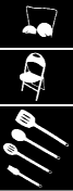
GT

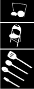
M³Net

SRformer

[32]

VST

[31]

Figure 2: Previous Transformer-based methods often suffer from a loss of local details, whereas our proposed M3Net excels at preserving these fine-grained details.

Our main contributions can be summarized as follows:

• Based on the feature pyramid structure, we rethink the uniqueness and independence between multiscale features and their distinctive contributions to final prediction, and accordingly propose a multiscale and multistage decoder. The decoder can optimize and integrate features step by step, and progressively reconstruct the saliency map.

• We introduce the Multilevel Interaction Block (MIB) to facilitate the interaction between features at different levels, specifically utilizing high-level features to guide the learning of low-level features. As demonstrated later, the MIB effectively enhances the salient region within the low-level features.

• We propose the Mixed Attention Block (MAB), which integrates self-attention and window self-attention mechanisms. The MAB enables improved localization of salient regions while preserving fine-grained object details.

Our proposed method differs distinctly from existing works in two key aspects. Firstly, in our multistage decoder, we adopt a sequential processing approach for features instead of the conventional two-dimensional form. As a result, no convolutional operations were incorporated into the decoder. Secondly, we capture the global and fine-grained features both through the attention mechanisms instead of adjusting the kernel size as done in many existing methods. Besides, We evaluate our model on six challenging datasets, and the results show that the M³Net achieves state-of-the-art results compared to recent competitive models.

II Related Work

II-A Convolution Based Methods

CNN-based methods are widely used in SOD and gain commendable performance, which usually takes the pre-trained networks [36, 37] as the encoder, and most of the efforts are then to design an effective decoder to conduct multilevel feature aggregation. Most methods [38, 14, 39] use the U-shape [13] based structures as the encoder-decoder architecture and progressively aggregate the hierarchical features for final prediction, while DSS [21] follows the HED [40] structure to fully utilize multilevel and multiscale features. Some methods tend to utilize the attention mechanism to learn more discriminative features, such as pixel-wise contextual attention [41], spatial and channel attention [20]. Multi-task learning is also widely used for SOD, including with the tasks, eye fixation prediction [42, 43], edge detection [18, 44, 45, 46], and image caption [47].

Unlike previous CNN-based methods, our M³Net can handle features extracted by Transformer as the encoder and performs sequential processing of feature maps in the decoder. We adopt the U-shape structure and consider the uniqueness and interdependence of multilevel features by implementing the proposed Multilevel Interaction Block, thus facilitating the subsequent aggregation of multilevel features. In addition, we employ the ”fold with overlap” as the upsampling method for our token-based model and perform a comparison with other existing upsampling methods.

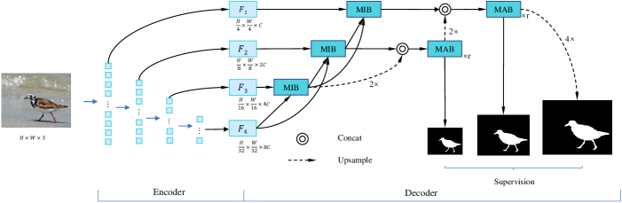
Figure 3: Overall architecture of our proposed M³Net model for salient object detection. The backbone is defined as a hierarchical network structure (e.g. ResNet[36], SwinTransformer[35]).

II-B Transformer Based Methods

Transformer encoder-decoder architecture was first proposed by Vaswani et al. [48] for natural language processing. Since the success of ViT [27] in image classification, more and more works have introduced Transformer architecture to computer vision tasks. SETR [28] and PVT [49] use ViT as the encoder for semantic segmentation. In SOD, VST [31] employs T2T-ViT [50] as the backbone and proposes an effective multi-task decoder for features in a sequence form. SRformer [32] adopted PVT as the encoder backbone and uses pixel shuffle as the upsampling method. Besides, HRTransNet [33] explored the application of transformer in two-modality SOD tasks, such as RGB-D SOD and RGB-T SOD.

Previous Transformer-based methods are superior in locating and capturing the salient areas in the images, while the details at the local level could be ignored. Inspired by the success of window self-attention [35], we introduce window self-attention in our decoder to strengthen the ability to model local context. As shown in Figure 2, our M³Net can model context at both global and local levels, thus effectively preserving local details on the basis of localized salient objects.

II-C Multilevel Feature Enhancement and Aggregation

Multilevel feature enhancement and aggregation are crucial for gaining a high-resolution saliency map, and numerous methods have thoroughly investigated them. GateNet[39] adopted the gate mechanism to balance the contribution of each encoder block and reduce non-salient information. MiNet [38] proposed an interactive learning method for multilevel features, aiming to minimize the discrepancies and improve the spatial coherence of multilevel features. ICON[51] incorporated convolution kernels with different shapes to enhance the diversity of multilevel features. BBRF[52] designed a switch-path decoder with various receptive fields to deal with large or small-scale objects.

To fully utilize multi-scale features, we first design the proposed Multiscale Interaction Block which introduces the cross-attention mechanism to achieve the interaction among multilevel features. In this mechanism, high-level features guide low-level feature learning from top to bottom. Then, in order to effectively integrate salient information across various scales within the aggregated features, we propose the Mixed Attention Block, which combines global self-attention and local window self-attention. This combination is aimed at modeling context at both global and local levels for further improvement in the accuracy of the prediction map.

III Proposed method

III-A Overview

The overall architecture of our proposed M³Net is given in Figure 3, which includes a Transformer encoder plus a multistage decoder with mixed attention. The encoder uses the Swin Transformer as the backbone for the demonstration of the proposed methodology, while any other hierarchical network models are applicable to extract multilevel features. The decoder optimizes and integrates multilevel features step by step, and gradually reconstructs the saliency map.

After obtaining multilevel features by the backbone, we optimize the features by passing them through the multiscale interaction block, which can enhance salient regions in low-level features. Then, on the basis of detected salient regions, we further use the mixed attention block to improve the local-level fine details of the saliency map. In addition, supervision is applied to each decoder level, aiming to facilitate the model training and improve the performance of the model.

III-B Swin Transformer Encoder

Transformer based on the standard architecture [27] has made competitive achievements in image classification, where the relationships between a token and all other tokens are computed. However, the vanilla Transformer has quadratic complexity. This limits it to be applied to many other vision problems such as SOD, which requires tremendous tokens for dense prediction or gaining a high-resolution image.

For efficient modeling, Swin Transformer uses window self-attention to replace standard global self-attention, reducing complexity to linear. To achieve information exchange among non-overlapping windows, shifted window partitioning is adopted, and the successive Swin Transformer blocks can be formulated as:

$$\small\begin{split}&\hat{\text{z}}^{l}=\text{W-MSA}(\text{LN}(\text{z}^{l-1}))+\text{z}^{l-1},\\ &\text{z}^{l}=\text{MLP}(\text{LN}(\hat{\text{z}}^{l}))+\hat{\text{z}}^{l},\\ &\hat{\text{z}}^{l+1}=\text{SW-MSA}(\text{LN}(\text{z}^{l}))+\text{z}^{l},\\ &\text{z}^{l+1}=\text{MLP}(\text{LN}(\hat{\text{z}}^{l+1}))+\hat{\text{z}}^{l+1},\end{split}$$ (1)

where $\hat{\text{z}}^{l}$ and $\text{z}^{l}$ denote the output features of the (S)W-MSA module and the MLP module for block $l$, respectively.

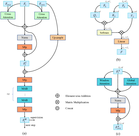
Figure 4: Details of our multistage decoder. (a) denotes one stage of the decoder, (b) denotes the structure of cross-attention, and (c) denotes the structure of the Mixed Attention Block. $r$ denotes the number of MAB stacked and we set it to 2. $F_{i+1}$ can be from $F^{I}_{i+1}$ or $F^{M}_{i+1}$.

Image

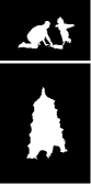
GT

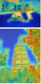
Before

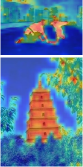
After

Figure 5: Visual comparison of our MIB where ‘Before’ denotes the features before MIB, and ‘After’ denotes the features after processed. The salient area has been observably enhanced, and meanwhile, local noises have also been effectively reduced.

III-C Multistage Decoder

Figure 4 shows the detail of our multistage decoder. As shown in Figure 4 (a), in one stage, we first let multilevel features interact across 2 scales to enhance the quality of low-level features. Then, we transform multilevel features to the same resolution by upsampling method. To better integrate salient information after feature fusion, we further perform mixed attention.

III-C1 Multilevel Interaction Block

We argue that low-level features contain more non-salient information and noise, and using an all-pass skip-layer structure to concatenate the low-level features of the encoder to the decoder may cause a negative impact on the saliency map. However, low-level features are rich in local spatial details, which is crucial to gain high quality saliency maps. Some methods [38, 51] rescale the adjacent levels of features and employ upsampling or downsampling operations to align them at the same spatial resolution, followed by concatenation for further processing. Nevertheless, the non-learnable nature of commonly used sampling operations (e.g., bilinear) leads to information loss, thereby limiting the model’s performance. To solve the loss of information during sampling, we propose our MIB block, which introduces the cross-attention mechanism to achieve the interaction of multilevel features, letting high-level features guide low-level features to strengthen salient regions and eliminate non-salient information. Through cross-attention, we can accomplish feature interaction across multiple scales without changing them in spatial resolution.

In the MIB block, given the features in a sequence form $F_{1}\in\mathbb{R}^{l_{1}\times c_{1}}$, $F_{2}\in\mathbb{R}^{l_{2}\times c_{2}}$, where $F_{1}$ denotes low-level features and $F_{2}$ denotes high-level features. We first change their channel dimension and embed them to queries $Q_{1}\in\mathbb{R}^{l_{1}\times d}$, keys $K_{2}\in\mathbb{R}^{l_{2}\times d}$, and values $V_{2}\in\mathbb{R}^{l_{2}\times d}$ through three linear projections. Then, we compute attention between the queries from low-level features with the keys from high-level features. The output is computed as a weighted sum of the values, formulated as:

$$\small\begin{split}\text{Attention}(Q_{1},K_{2},V_{2})=\text{Softmax}(Q_{1}K_{2}^{T}/\sqrt{d})V_{2}.\end{split}$$ (2)

As shown in Figure 4 (a), our MIB makes features interact across two scales. Two cross-attentions are performed in parallel and gathered by element-wise addition. We follow the standard Transformer architecture [48] in subsequent structure, including layer normalization [53], residual connections, formulated as:

$$\begin{split}&\hat{F}_{i}=F_{i}+\text{CA}(F_{i},F_{i+1})+\text{CA}(F_{i},F_{i+2}),\\ &F_{i}^{I}=\text{MLP}(\text{LN}(\hat{F}_{i}))+\hat{F}_{i},\end{split}$$ (3)

where $F_{i+1}$, $F_{i+2}$ denote the high-level features. $\hat{F}_{i}$, $F_{i}^{I}$ denote the output features of the cross-attention (CA) modules and the MLP module in the MIB, respectively.

By using the proposed MIB, the salient region at the global level can be effectively enhanced. As can be seen in Figure 5, after feeding the features into our MIB, the salient region is noticeably distinguished from the non-salient areas.

III-C2 Mixed Attention Block

To facilitate the aggregation of multilevel features in the sequence form,  [31] adopts one Transformer layer with global self-attention, which may neglect local-level details and limit the fineness of the final prediction. Inspired by the success of window self-attention [35], which computes self-attention within local windows, we combine global self-attention and window self-attention, aiming to model context at both global and local levels, further improve the local accuracy of the prediction map. We use the same window size (set to $7\times 7$ by default) as the encoder.

As can be seen in Figure 4 (a), given feature in a sequence form $F_{i}^{C}\in\mathbb{R}^{l\times c}$ after feature fusion, we first increase its channel dimension to $d=384$ by an MLP, and then let it pass $r$ mixed attention blocks. Similar to our MIB, window self-attention and global self-attention are performed in parallel, and gathered by element-wise addition, followed by standard Transformer architecture. Finally, we apply another MLP to restore the channel dimension of the feature for subsequent processing and supervision. The whole process can be formulated as:

$$\begin{split}&F_{0}^{A}=\text{MLP}_{1}(F_{i}^{I}),\\ &\hat{F}_{1}^{A}=\text{W-MSA}(F_{0}^{A})+\text{MSA}(F_{0}^{A}),\\ &F_{1}^{A}=\text{MLP}(\text{LN}(\hat{F}_{1}^{A}))+\hat{F}_{1}^{A},\\ &\qquad...\\ &F_{i}^{M}=\text{MLP}_{2}(F_{r}^{A}),\\ \end{split}$$ (4)

where $\hat{F}_{i}^{A}$ and $F_{i}^{A}$ denote the output features of the mixed attention module and the MLP module in our MABs, respectively. $r$ denotes the number of MAB stacked and we set it to 2.

III-C3 Upsampling Methods and Multilevel Fusion

TABLE I: Quantitative comparison of our proposed M³Net with other 16 SOTA SOD methods on six benchmark datasets. The symbols “↑”/“↓” mean that a higher/lower score is better. The best results are shown in bold. ‘-R’, ’-R2’, and ‘-S’ means the ResNet50, Res2Net50[54], and SwinTransformer backbone.

dataset	DUT-O				DUTS				ECSSD				HKU-IS				PASCAL-S				SOD
Method	$M\downarrow\>$	$E_{\xi}^{m}\uparrow\>$	$S_{m}\uparrow\>$	$F_{\beta}^{w}\uparrow\>$	$M\downarrow\>$	$E_{\xi}^{m}\uparrow\>$	$S_{m}\uparrow\>$	$F_{\beta}^{w}\uparrow\>$	$M\downarrow\>$	$E_{\xi}^{m}\uparrow\>$	$S_{m}\uparrow\>$	$F_{\beta}^{w}\uparrow\>$	$M\downarrow\>$	$E_{\xi}^{m}\uparrow\>$	$S_{m}\uparrow\>$	$F_{\beta}^{w}\uparrow\>$	$M\downarrow\>$	$E_{\xi}^{m}\uparrow\>$	$S_{m}\uparrow\>$	$F_{\beta}^{w}\uparrow\>$	$M\downarrow\>$	$E_{\xi}^{m}\uparrow\>$	$S_{m}\uparrow\>$	$F_{\beta}^{w}\uparrow\>$
CNN Methods
PiCANet	.054	.865	.826	.743	.04	.915	.863	.812	.035	.953	.916	.908	.031	.951	.905	.89	.064	.9	.846	.811	.094	.846	.78	.741
BASNet	.056	.871	.836	.751	.048	.903	.866	.803	.037	.951	.916	.904	.032	.951	.909	.889	.076	.886	.838	.793	.112	.832	.772	.728
CPD-R	.056	.868	.825	.719	.043	.914	.869	.795	.037	.951	.918	.898	.034	.95	.905	.875	.071	.891	.848	.794	.11	.849	.771	.713
PoolNet	.054	.867	.831	.725	.037	.926	.887	.817	.035	.956	.926	.904	.03	.958	.919	.888	.065	.907	.865	.809	.103	.867	.792	.746
AFNet	.057	.861	.826	.717	.046	.91	.867	.785	.042	.947	.913	.886	.036	.949	.905	.869	.07	.895	.849	.797	.108	.847	.78	.726
EGNet	.053	.878	.841	.738	.039	.927	.887	.816	.037	.955	.925	.903	.031	.958	.918	.887	.074	.892	.852	.795	.097	.873	.807	.767
ITSD-R	.061	.88	.84	.75	.041	.929	.885	.824	.034	.959	.925	.91	.031	.96	.917	.894	.066	.908	.859	.812	.093	.873	.809	.777
MINet-R	.056	.869	.833	.738	.037	.927	.884	.825	.033	.957	.925	.911	.029	.96	.919	.897	.064	.903	.856	.809	.092	.87	.805	.768
LDF	.052	.869	.839	.752	.034	.93	.892	.845	.034	.954	.924	.915	.028	.958	.919	.904	.06	.908	.863	.822	.093	.866	.8	.765
CSF-R2	.055	.775	.838	.733	.037	.93	.89	.823	.033	.96	.93	.91	.03	.96	.921	.891	.069	.899	.862	.807	.098	.872	.8	.757
GateNet-R	.055	.876	.838	.729	.04	.928	.885	.809	.04	.952	.92	.894	.033	.955	.915	.88	.067	.904	.858	.797	.098	.87	.801	.753
PFSNet	.055	.878	.842	.756	.036	.931	.892	.842	.031	.958	.93	.92	.026	.962	.924	.91	.063	.906	.86	.819	.089	.875	.81	.781
ICON-R	.057	.884	.844	.761	.037	.932	.889	.837	.032	.96	.929	.918	.029	.96	.92	.902	.064	.908	.861	.818	.084	.882	.824	.794
M3Net-R	.061	.88	.848	.769	.036	.937	.897	.849	.029	.962	.931	.919	.026	.966	.929	.913	.06	.912	.868	.827	.084	.865	.819	.784
Transformer Methods
VST	.058	.89	.852	.758	.037	.94	.897	.831	.032	.965	.934	.911	.029	.968	.928	.897	.06	.919	.874	.821	.085	.876	.82	.776
ICON-S	.043	.906	.869	.804	.025	.96	.917	.886	.023	.972	.941	.936	.022	.974	.935	.925	.048	.93	.885	.854	.083	.885	.825	.802
SRformer	.043	.894	.86	.784	.027	.952	.91	.872	.028	.961	.932	.922	.025	.966	.928	.912	.051	.924	.878	.845	.088	.862	.809	.77
BBRF	.044	.899	.861	.803	.025	.952	.909	.886	.022	.972	.939	.944	.02	.972	.932	.932	.049	.927	.878	.856	.078	.868	.822	.802
M3Net-S	.045	.903	.872	.811	.024	.96	.927	.902	.021	.974	.948	.947	.019	.977	.943	.937	.047	.932	.889	.864	.073	.871	.838	.819

Most CNN-based methods [51, 38] adopt bilinear interpolation to re-scale high resolution feature maps, while upsampling features in the sequence form remain under-studied. In this work, we adopt the RT2T method developed in  [31, 50] for token upsampling, where we found that fold with overlap leads to other upsampling methods not only in evaluation indicators but also in the visual quality of saliency map.

We first use a linear projection to expand the channel dimension of $F_{i}^{I}\in\mathbb{R}^{l\times c}$ to $ck^{2}$. Each token is seen as a $k\times k$ image patch and neighboring patches have $k-s$ overlapping, where $s$ denotes the stride. Then we fold the tokens with $p$ zero-padding. The arguments need to satisfy:

$$\small\begin{split}l=h\times w=\lfloor\frac{h_{o}+2p-k}{s}+1\rfloor\times\lfloor\frac{w_{o}+2p-k}{s}+1\rfloor,\end{split}$$ (5)

where $h_{o}\times w_{o}$ denotes the spatial size of the feature maps after folding. We reshape the feature map to the tokens with the size $l_{o}\times c$, where $l_{o}=h_{o}\times w_{o}$, and define it as $F_{i}^{U}$. We follow  [31] to set $k=[3,3,7]$, $s=[2,2,4]$, and $p=[1,1,2]$ to get the same resolution as the original input image after three times upsampling. The upsampling ratio of each time is equal to the stride.

As can be seen in Figure 4 (a), we fuse multilevel features after upsampling high-level features, and then use our MABs to further integrate salient information at different levels. One whole stage of the decoder can be formulated as:

$$\begin{split}&F_{i+1}^{U}=\text{Upsample}(F_{i+1}^{M}),\\ &F_{i}^{I}=\text{MIB}(F_{i},F_{i+1},F_{i+2}),\\ &F_{i}^{C}=\text{Concat}(F_{i}^{I},F_{i+1}^{U}),\\ &F_{i}^{M}=\text{MAB}s(F_{i}^{C}),\end{split}$$ (6)

where $F_{i+1}^{M}$ denotes the output of previous stage ($F_{3}$ employed in the first stage) and $F_{i}^{C}$ denotes the feature maps after fusing. $F_{i}^{M}$ will be used for the next stage of the decoder and the multilevel supervision.

III-C4 Multilevel Supervision Strategy

TABLE II: Comparison of our proposed model with other SOTA CNN-based SOD methods on SOC test set. The best results are shown in bold.

Attr	Metrics	Amulet	DSS	NLDF	C2SNet	SRM	R3Net	BMPM	DGRL	PiCA-R	RANet	AFNet	CPD	PoolNet	EGNet	BANet	SCRN	ICON-R	Ours-R
AC	$M\downarrow\>$	.120	.113	.119	.109	.096	.135	.098	.081	.093	.132	.084	.083	.094	.085	.086	.078	.062	.071
	$E_{\xi}^{m}\uparrow\>$	.791	.788	.784	.807	.824	.753	.815	.853	.815	.765	.852	.843	.846	.854	.858	.849	.891	.885
	$S_{m}\uparrow\>$	.752	.753	.737	.755	.791	.713	.780	.790	.792	.708	.796	.799	.795	.806	.806	.809	.835	.824
	$F_{\beta}^{w}\uparrow\>$	.620	.629	.620	.647	.690	.593	.680	.718	.682	.603	.712	.727	.713	.731	.740	.724	.784	.764
BO	$M\downarrow\>$	.346	.356	.354	.267	.306	.445	.303	.215	.200	.454	.245	.257	.353	.373	.271	.224	.200	.199
	$E_{\xi}^{m}\uparrow\>$	.551	.537	.539	.661	.616	.419	.620	.725	.741	.404	.698	.665	.554	.528	.650	.706	.740	.763
	$S_{m}\uparrow\>$	.574	.561	.568	.654	.614	.437	.604	.684	.729	.421	.658	.647	.561	.528	.645	.698	.714	.704
	$F_{\beta}^{w}\uparrow\>$	.612	.614	.622	.730	.667	.456	.670	.786	.799	.453	.741	.739	.610	.585	.720	.778	.794	.783
CL	$M\downarrow\>$	.141	.153	.159	.144	.134	.182	.123	.119	.123	.188	.119	.114	.134	.139	.117	.113	.113	.112
	$E_{\xi}^{m}\uparrow\>$	.789	.763	.764	.789	.793	.710	.801	.824	.794	.715	.802	.821	.801	.790	.824	.820	.829	.832
	$S_{m}\uparrow\>$	.763	.722	.713	.742	.759	.659	.761	.770	.787	.624	.768	.773	.760	.757	.784	.795	.789	.791
	$F_{\beta}^{w}\uparrow\>$	.663	.617	.614	.655	.665	.546	.678	.714	.692	.542	.696	.724	.681	.677	.726	.717	.732	.736
HO	$M\downarrow\>$	.119	.124	.126	.123	.115	.136	.116	.104	.108	.143	.103	.097	.100	.106	.094	.096	.092	.091
	$E_{\xi}^{m}\uparrow\>$	.810	.796	.798	.805	.819	.782	.813	.833	.819	.777	.834	.845	.846	.829	.850	.842	.852	.865
	$S_{m}\uparrow\>$	.791	.767	.755	.768	.794	.740	.781	.791	.809	.713	.798	.803	.815	.802	.819	.823	.818	.823
	$F_{\beta}^{w}\uparrow\>$	..688	.660	.661	.668	.696	.633	.684	.722	.704	.626	.722	.751	.739	.720	.754	.743	.752	.767
MB	$M\downarrow\>$	.142	.132	.138	.128	.115	.160	.105	.113	.099	.139	.111	.106	.121	.109	.104	.100	.100	.077
	$E_{\xi}^{m}\uparrow\>$	.739	.753	.740	.778	.778	.697	.812	.823	.813	.761	.762	.804	.779	.789	.803	.817	.828	.88
	$S_{m}\uparrow\>$	.712	.719	.685	.720	.742	.657	.762	.744	.775	.696	.734	.754	.751	.762	.764	.792	.774	.819
	$F_{\beta}^{w}\uparrow\>$	.561	.577	.551	.593	.619	.489	.651	.655	.637	.576	.626	.679	.642	.649	.672	.690	.699	.74
OC	$M\downarrow\>$	.143	.144	.149	.130	.129	.168	.119	.116	.119	.169	.109	.115	.119	.121	.112	.111	.106	.99
	$E_{\xi}^{m}\uparrow\>$	.763	.760	.755	.784	.780	.706	.800	.808	.784	.718	.820	.810	.801	.798	.809	.800	.817	.843
	$S_{m}\uparrow\>$	.735	.718	.709	.738	.749	.653	.752	.747	.765	.641	.771	.750	.756	.754	.765	.775	.771	.786
	$F_{\beta}^{w}\uparrow\>$	.607	.595	.593	.622	.630	.520	.644	.659	.638	.527	.680	.672	.659	.658	.678	.673	.683	.709
OV	$M\downarrow\>$	.173	.180	.184	.159	.150	.216	.136	.125	.127	.217	.129	.134	.148	.146	.119	.126	.120	.109
	$E_{\xi}^{m}\uparrow\>$	.751	.737	.736	.790	.779	.663	.807	.828	.810	.664	.817	.803	.795	.802	.835	.808	.834	.838
	$S_{m}\uparrow\>$	.721	.700	.688	.728	.745	.624	.751	.762	.781	.611	.761	.748	.747	.752	.779	.774	.779	.795
	$F_{\beta}^{w}\uparrow\>$	.637	.622	.616	.671	.682	.527	.701	.733	.721	.529	.723	.721	.697	.707	.752	.723	.749	.759
SC	$M\downarrow\>$	.098	.098	.101	.100	.090	.114	.081	.087	.093	.110	.076	.080	.075	.083	.078	.078	.080	.078
	$E_{\xi}^{m}\uparrow\>$	.794	.799	.788	.806	.814	.765	.841	.837	.799	.792	.854	.858	.856	.844	.851	.843	.860	.871
	$S_{m}\uparrow\>$	.768	.761	.745	.756	.783	.716	.799	.772	.784	.724	.808	.793	.807	.793	.807	.809	.803	.808
	$F_{\beta}^{w}\uparrow\>$	.608	.599	.593	.611	.638	.550	.677	.669	.627	.594	.696	.708	.695	.678	.706	.691	.714	.714
SO	$M\downarrow\>$	.119	.109	.115	.116	.099	.118	.096	.092	.095	.113	.089	.091	.087	.098	.090	.082	.087	.079
	$E_{\xi}^{m}\uparrow\>$	.745	.756	.747	.752	.769	.732	.780	.802	.766	.759	.792	.804	.814	.784	.801	.797	.816	.835
	$S_{m}\uparrow\>$	.718	.713	.703	.706	.737	.682	.732	.736	.748	.682	.746	.745	.768	.749	.755	.767	.763	.778
	$F_{\beta}^{w}\uparrow\>$	.523	.524	.526	.531	.561	.487	.567	.602	.566	.518	.596	.623	.626	.594	.621	.614	.634	.66

After each stage of our multistage decoder, the channel of features will be reduced to 1-dimension, expressed as $F_{i}^{P}\in\mathbb{R}^{l\times 1}$, for multilevel supervision. Previous methods mostly apply BCE as the loss function, which treats every pixel equally and may neglect the relation between pixels. We additionally use the IoU loss [18, 55] to supervise the structural inconsistency between the prediction and the ground truth. The BCE loss is defined as:

$$\small\begin{split}\mathcal{L}_{BCE}=-\sum_{x=1}^{H}\sum_{y=1}^{W}[G(x,y)logP(x,y)\\ +(1-G(x,y))log(1-P(x,y))],\end{split}$$ (7)

where $H$, $W$ are the height and width of the image, and $P(x,y)$, $G(x,y)$ denote the pixels of the prediction and the ground truth at position $(x,y)$, respectively. Meanwhile, the IoU loss is formulated as:

$$\small\begin{split}\mathcal{L}_{IoU}=1-\frac{\sum_{x=1}^{H}\sum_{y=1}^{W}(P(x,y)G(x,y))}{\sum_{x=1}^{H}\sum_{y=1}^{W}(P(x,y)+G(x,y)-P(x,y)G(x,y))},\end{split}$$ (8)

Then the joint loss can be defined as:

$$\small\begin{split}\mathcal{L}(P,G)=\mathcal{L}_{BCE}+\mathcal{L}_{IoU}.\end{split}$$ (9)

During training, we also use the multilevel supervision strategy widely used in [56, 38, 57, 58, 31] to facilitate the training process.

IV Experiments

IV-A Implementation Details

For fair comparison, we follow recent methods to use the DUTS-TR (10553 images) [59] to train our M³Net and we resize images to 224×224. Normalization, random $90^{\circ}$ rotation, and crop were applied as the data augmentation. According to  [60], we set the batch size as 8 to avoid weakening the generalization ability of the model. We use the Adam optimizer to train our network for 120 epochs and set its initial learning rate to 0.0001. In order to make the model converge better, we reduce the learning rate to 0.00002 in the last 20 epochs. All experiments were implemented on an RTX 3090 GPU.

IV-B Evaluation Datasets and Metrics

We evaluate our M³Net on six widely used benchmark datasets, including DUT-OMORN [61] (5168 images), DUTS-TE [59] (5019 images), ECSSD [62] (1000 images), HKU-IS [63] (4447 images), PASCAL-S [64] (850 images), SOD [65] (300 images).

We use four metrics to evaluate our model and the existing state-of-the-art algorithms:

(1) MAE. MAE evaluates the average pixel-wise difference between the prediction $P$ and the ground-truth $G$, and is computed as $MAE=\frac{1}{H\times W}\sum_{x=1}^{H}\sum_{y=1}^{W}|P(x,y)-G(x,y)|$.

(2) E-measure. E-measure [66] considers the local pixel values with the image-level mean value simultaneously: $E_{\xi}=\frac{1}{H\times W}\sum_{x=1}^{H}\sum_{y=1}^{W}\phi_{\xi}(i,j)$ where $\phi_{\xi}$ denotes the enhanced alignment matrix.

(3) S-measure. S-measure [67] aims to measure the structural similarity between the prediction and ground truth, which is computed as $S_{m}=\alpha S_{o}+(1-\alpha)S_{r}$. $S_{o}$ and $S_{r}$ denote the object-level and region-level structural similarity, respectively, and $\alpha$ is set to 0.5.

(4) Weighted F-measure. Weighted F-measure [68] gives an intuitive generalization of $F_{\beta}$, calculated as $F_{\beta}^{w}=\frac{(1+\beta^{2})\times Precision^{w}\times Recall^{w}}{\beta^{2}\times Precision^{w}+Recall^{w}}$. It extends the four basic quantities TP, TN, FP and FN to real values, and assigns different weights $(w)$ to different errors based on different locations and neighborhood information.

IV-C Comparison with State-of-the-Art

TABLE III: The performance of our model under different inputs and backbones with varying scales.

Method	Backbone	Input Size	MACs	Params	DUTS				ECSSD				HKU-IS
					$M\downarrow\>$	$E_{\xi}^{m}\uparrow\>$	$S_{m}\uparrow\>$	$F_{\beta}^{w}\uparrow\>$	$M\downarrow\>$	$E_{\xi}^{m}\uparrow\>$	$S_{m}\uparrow\>$	$F_{\beta}^{w}\uparrow\>$	$M\downarrow\>$	$E_{\xi}^{m}\uparrow\>$	$S_{m}\uparrow\>$	$F_{\beta}^{w}\uparrow\>$
Ours-R	ResNet50	224$\times$224	18.83	34.61	0.036	0.937	0.897	0.849	0.029	0.962	0.931	0.919	0.026	0.966	0.929	0.913
Ours-R	ResNet50	352$\times$352	46.49	34.61	0.039	0.931	0.898	0.856	0.03	0.959	0.932	0.923	0.025	0.964	0.93	0.916
Ours-S	SwinS	224$\times$224	23.11	59.07	0.028	0.952	0.913	0.878	0.024	0.97	0.941	0.935	0.023	0.97	0.934	0.921
Ours-S	SwinB	224$\times$224	39.51	102.62	0.026	0.955	0.918	0.885	0.022	0.974	0.945	0.941	0.021	0.975	0.939	0.928
Ours-S	SwinB	384$\times$384	116.12	102.75	0.024	0.96	0.927	0.902	0.021	0.974	0.948	0.947	0.019	0.977	0.943	0.937

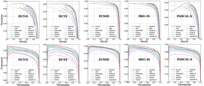
Figure 6: Precision-Recall curves (row 1) and F-measure curves (row 2) of our M³Net-R and other CNN SOTA methods on five benchmark datasets.

Image

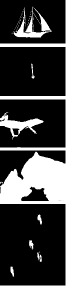
GT

M³Net-S

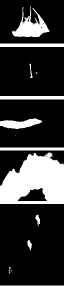
BBRF

[52]

ICON-S

[51]

SRformer

[32]

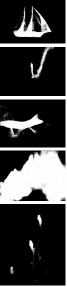
VST

[31]

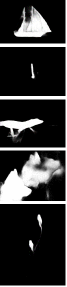
GateNet

[39]

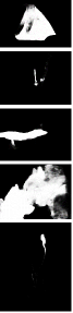
MiNet

[38]

F3Net

[57]

Figure 7: Visual comparisons between our M³Net and other 7 state-of-the-art methods on various scenes. In contrast to previous methods, our M³Net generates prediction maps with fewer shadows and undersaturated regions, thereby enhancing its reliability.

We compare our M³Net with 30 state-of-the-art methods, including PiCANet [41], RAS [69], Amulet[14], DSS[21], NLDF[70], C2SNet[71], SRM[72], R3Net[73], BMPM[74], DGRL[75], RANet[76], BANet[77], BASNet [18], CPD [19], PoolNet [56], AFNet [78], TSPOANet [79], EGNet [44], SCRN [80], F3Net [57], ITSD [81], MiNet [38], LDF [82], CSF [83], GateNet [39], PFSNet[84], ICON [51], VST [31], SRformer [32] and BBRF[52]. We also adopt ResNet-50 as the backbone to compare with CNN-based methods, in which case our model is referred to as M³Net-R.

IV-C1 Quantitative Comparison

Table I shows the quantitative comparison results on six widely used benchmark datasets. We compare our method with 16 state-of-the-art methods in terms of MAE, $E_{\xi}$, $S_{m}$, $F_{\beta}^{w}$. Regarding M³Net-R, an input size of 224 x 224 is adopted. In the case of M³Net-S, an input size of 384 x 384 is used. The results show that our M³Net not only outperforms all previous state-of-the-art Transformer based methods but also achieves competitive results in CNN-based methods. We also report the performance of our model under different inputs and backbones with varying scales. As shown in Table III, with the increase in the size of the input image, both the performance and computational cost of the model increase simultaneously. Therefore, we can adjust the input size of the model to accommodate different computational requirements. In addition, we present the precision-recall [85] and F-measure curves [86] in Figure 6.

Recently, Fan et al. proposed a challenging dataset known as SOC[87], which is based on real-world scenarios. In contrast to previous datasets, the SOC dataset comprises more complex scenes and is divided into nine distinct subsets based on image attributes, including AC (appearance change), BO (big object), CL (clutter), HO (heterogeneous object), MB (motion blur), OC (occlusion), OV (out-of-view), SC (shape complexity), and SO (small object). Evaluating the performance of our proposed model in comparison to previous methods on the SOC dataset provides a more comprehensive validation of its performance. Table II presents a comparison between our model and 17 recent state-of-the-art CNN-based methods, focusing on attribute-based performance. Notably, our model demonstrates significant performance improvement compared to the existing methods.

IV-C2 Visual Comparison

Figure 7 provides visual comparisons between our method and other methods. As can be seen, our M³Net reconstructs more accurate saliency maps, while local fine-grained details are well preserved. Besides, our method excels in dealing with challenging cases like small objects (row 2), low-contrast (row 4), complex backgrounds (row 3), delicate structures (row 1), and multiple objects (rows 4 and 5) integrally and noiselessly. The above results show the versatility and robustness of our M³Net.

IV-D Ablation Studies

TABLE IV: Ablation studies of our proposed model. “Bi” denotes bilinear upsampling, “F” denotes fold upsampling, “MIB” denotes our proposed multilevel interaction block, and “MAB” denotes our proposed mixed attention block.

ID	Component Settings	DUTS				ECSSD				HKU-IS
		$M\downarrow\>$	$E_{\xi}^{m}\uparrow\>$	$S_{m}\uparrow\>$	$F_{\beta}^{w}\uparrow\>$	$M\downarrow\>$	$E_{\xi}^{m}\uparrow\>$	$S_{m}\uparrow\>$	$F_{\beta}^{w}\uparrow\>$	$M\downarrow\>$	$E_{\xi}^{m}\uparrow\>$	$S_{m}\uparrow\>$	$F_{\beta}^{w}\uparrow\>$
1	+Bi	0.046	0.9	0.851	0.78	0.046	0.936	0.897	0.879	0.035	0.945	0.896	0.872
2	+F	0.042	0.911	0.868	0.802	0.042	0.939	0.906	0.888	0.031	0.953	0.911	0.888
3	+F+MIB	0.038	0.93	0.891	0.84	0.035	0.953	0.923	0.907	0.028	0.96	0.923	0.904
4	+F+MAB	0.037	0.933	0.892	0.842	0.035	0.953	0.924	0.908	0.028	0.961	0.923	0.904
5	+F+MIB+MAB	0.036	0.937	0.897	0.849	0.029	0.962	0.931	0.919	0.026	0.966	0.929	0.913

TABLE V: Ablation Studies of different feature enhancement methods compared with our MIB.

ID	FEMs Settings	DUTS			ECSSD			HKU-IS
		$M\downarrow$	$S_{m}\uparrow$	$F_{\beta}^{w}\uparrow$	$M\downarrow$	$S_{m}\uparrow$	$F_{\beta}^{w}\uparrow$	$M\downarrow$	$S_{m}\uparrow$	$F_{\beta}^{w}\uparrow$
3	MIB	.038	.891	.84	.035	.923	.907	.028	.923	.904
6	DFA[51]	.045	.878	.796	.04	.92	.892	.035	.915	.88
7	RFB[88]	.043	.882	.807	.039	.921	.893	.035	.915	.88
8	AIM[38]	.041	.888	.809	.037	.923	.898	.033	.919	.887

TABLE VI: Different cross-levels in our MIB.

ID	Across Levels	DUTS			ECSSD			HKU-IS
		$M\downarrow$	$S_{m}\uparrow$	$F_{\beta}^{w}\uparrow$	$M\downarrow$	$S_{m}\uparrow$	$F_{\beta}^{w}\uparrow$	$M\downarrow$	$S_{m}\uparrow$	$F_{\beta}^{w}\uparrow$
3	2	.038	.891	.84	.035	.923	.907	.028	.923	.904
9	1	.039	.889	.837	.034	.923	.906	.029	.922	.904
10	3	.039	.887	.835	.037	.92	.906	.03	.922	.903

TABLE VII: Different interaction modes in our MIB.

ID	Interaction Settings	DUTS			ECSSD			HKU-IS
		$M\downarrow$	$S_{m}\uparrow$	$F_{\beta}^{w}\uparrow$	$M\downarrow$	$S_{m}\uparrow$	$F_{\beta}^{w}\uparrow$	$M\downarrow$	$S_{m}\uparrow$	$F_{\beta}^{w}\uparrow$
3	high to low	.038	.891	.84	.035	.923	.907	.028	.923	.904
11	low to high	.042	.886	.836	.038	.911	.898	.031	.914	.891
12	bi-directional	.039	.889	.837	.036	.923	.907	.029	.922	.902

To demonstrate the effectiveness of different modules in our M³Net, we conduct the quantitative results of several simplified versions of our method. The experimental results on three datasets including DUTS-TE, ECSSD, HKU-IS are given in Table IV. We start from a UNet-like structure with skip connections and bilinear upsampling as the baseline and progressively incorporate the proposed modules, including MIB and MAB.

IV-D1 Effectiveness of MIB

For enhancing multilevel features from the encoder, we use our MIB to strengthen salient regions and reduce non-salient information of low-level features, shown as “+MIB” in Table 2. The results show that our MIB gains notable improvement, demonstrating its effectiveness.

To verify the superiority of the proposed MIB, we compared it with existing feature enhancement methods, including DFA[51], RFB[88], and AIM[38]. As can be seen in Table V, the proposed MIB demonstrates advantages across all performance metrics. This suggests that utilizing the complementarity of multiscale features can lead to improved feature enhancement effects.

To further investigate the effectiveness of our MIB and the interaction between multilevel features, we made adjustments to the scale range of the MIB. For instance, when we combine two scales, we employ features at 1/8 and 1/16 levels to interact with features at the 1/4 level. Conversely, when we intersect two scales, we exclusively use features at the 1/8 level to interact with features at the 1/4 level. The results are presented in Table VI.

It is worth mentioning that the interaction within our MIB is unidirectional, where the high-level features solely guide the low-level features. Hence, we also endeavored to integrate reverse and bidirectional interaction in our MIB, and the outcomes are showcased in Table VII. The low-to-high interaction is observed to result in performance degradation, which could be attributed to the presence of noise and non-salient information in the low-level features.

IV-D2 Effectiveness of MAB

To better integrate salient information from multilevel features after fusing them, we use our MABs to model context at both global and local levels to gain high quality salient map, shown as “+MAB” in Table IV. The results demonstrate the effectiveness of our MAB.

In order to demonstrate the superior performance of the proposed MAB in saliency integration, we conduct a comparative evaluation with existing methods, including SIM[38], AFM[89], shown as Table VIII. The effectiveness of the proposed MAB in integrating salient information while preserving intricate local details is evident, resulting in the generation of saliency predictions of high quality.

To further explore the effectiveness of mixed attention, we conduct extra experiments, the results are shown in Table IX and Figure 8. We find that mixed attention can better retain local details with a slight additional computational cost. Besides, $7\times 7$ is also a more suitable window size.

Image

GT

Window

Global

Mixed

Figure 8: Visual comparison of the ablation study on our MAB. It can be seen that the mixed attention, which combines window attention and global attention, can not only ensure accurate object localization but also effectively preserve local details.

TABLE VIII: Ablation studies of different saliency integration methods compared with our MAB.

ID	Integration Methods	DUTS			ECSSD			HKU-IS
		$M\downarrow$	$S_{m}\uparrow$	$F_{\beta}^{w}\uparrow$	$M\downarrow$	$S_{m}\uparrow$	$F_{\beta}^{w}\uparrow$	$M\downarrow$	$S_{m}\uparrow$	$F_{\beta}^{w}\uparrow$
5	MAB	.036	.897	.849	.029	.931	.919	.026	.929	.913
13	SIM[38]	.037	.895	.834	.035	.925	.904	.032	.921	.893
14	AFM[89]	.04	.894	.837	.036	.923	.901	.031	.923	.894

TABLE IX: Ablation study of different attention settings in our MAB. $h\times w$ can be seen as global self-attention.

ID	Attention Settings	DUTS			ECSSD			HKU-IS
		$M\downarrow$	$S_{m}\uparrow$	$F_{\beta}^{w}\uparrow$	$M\downarrow$	$S_{m}\uparrow$	$F_{\beta}^{w}\uparrow$	$M\downarrow$	$S_{m}\uparrow$	$F_{\beta}^{w}\uparrow$
15	$h\times w$	.036	.894	.844	.03	.929	.918	.027	.927	.91
16	$7\times 7$	.038	.895	.843	.029	.929	.917	.028	.927	.908
5	$7\times 7+h\times w$	.036	.897	.849	.029	.931	.919	.026	.929	.913
17	$4\times 4+h\times w$	.038	.891	.839	.03	.929	.917	.028	.926	.906
18	$14\times 14+h\times w$	.036	.896	.847	.029	.931	.918	.027	.928	.91
19	$7\times 7+14\times 14$	.036	.894	.845	.03	.929	.917	.026	.926	.909

IV-D3 Evaluation of upsampling method

TABLE X: Ablation studies of the upsampling methods adopted in the M³Net.

ID	Upsampling Methods	DUTS			ECSSD			HKU-IS
		$M\downarrow$	$S_{m}\uparrow$	$F_{\beta}^{w}\uparrow$	$M\downarrow$	$S_{m}\uparrow$	$F_{\beta}^{w}\uparrow$	$M\downarrow$	$S_{m}\uparrow$	$F_{\beta}^{w}\uparrow$
20	pixel shuffle	.036	.895	.845	.031	.928	.915	.027	.926	.907
21	bilinear	.037	.89	.837	.031	.927	.914	.028	.923	.903
22	fold	.037	.893	.843	.029	.93	.917	.026	.927	.91
5	fold with overlap	.036	.897	.849	.029	.931	.919	.026	.929	.913

Image

GT

Fold with overlap

Fold

Bilinear

Pixel shuffle

Figure 9: Visual comparisons of upsampling methods. As can be observed, the prediction imaps obtained through upsampling with Fold and Pixel Shuffle exhibit undersaturation issues, while Bilinear interpolation results in a notable loss of local details.

TABLE XI: Ablation study of different loss function settings with our M³Net.

ID	Loss Settings	DUTS			ECSSD			HKU-IS
		$M\downarrow$	$S_{m}\uparrow$	$F_{\beta}^{w}\uparrow$	$M\downarrow$	$S_{m}\uparrow$	$F_{\beta}^{w}\uparrow$	$M\downarrow$	$S_{m}\uparrow$	$F_{\beta}^{w}\uparrow$
23	$\mathcal{L}_{bce}$	.039	.895	.835	.032	.93	.909	.029	.928	.903
5	$\mathcal{L}_{bce}+\mathcal{L}_{iou}$	.036	.897	.849	.029	.931	.919	.026	.929	.913
24	$\mathcal{L}_{wbce}+\mathcal{L}_{wiou}$[57]	.038	.895	.846	.03	.93	.917	.027	.927	.909

Upsampling methods for features in the form of a sequence remain under studied. We compare several widely used upsampling methods with our M³Net, including bilinear, pixel shuffle, and fold. The results are shown in Table X and Fig 9. From the comparison result, we found that fold with overlap not only leads in evaluation metrics but also makes the predicted saliency map closest to the real one.

IV-D4 Evaluation of Loss Function

We use different loss functions to train our M³Net, and the results are shown in Table XI. We find that the model supervised by BCE loss is weak in $F_{\beta}^{w}$ [68], which may be caused by BCE ignoring the relations between pixels, while IoU loss based on the whole region, effectively made up for the deficiencies of BCE loss. $\mathcal{L}_{wBCE}$ and $\mathcal{L}_{wIoU}$ [57] assign different weights to different regions, aiming to let the model pay more attention to complex regions. However, as shown in Table XI, it has not brought visible improvement to the performance of our model. We speculate that this lack of improvement may stem from the model’s pre-existing proficiency in attending to complex regions. Consequently, the emphasis on complex regions driven by weighted loss has the potential to impede the model’s perception of non-complex regions.

V Conclusion

In this paper, we propose a novel Transformer based network dubbed M³Net for SOD. Considering the uniqueness and interdependence of multilevel features, we first propose the MIB to achieve the interaction between multilevel features and thus enhance the localized salient regions in low-level features. Secondly, we design the MAB which integrates the global and window self-attentions, aiming at modeling local context to refine the fine-grained details of the objects. Finally, we design a multistage decoder by employing the MIB and MAB blocks and optimize the multilevel features step by step. Our M³Net model achieves state-of-the-art results on six challenging datasets without relying on heavy numerical computations, thus showing great potential for the SOD task in practical application.

References

- [1] Y. Liu, J. Han, Q. Zhang, and L. Wang, “Salient object detection via two-stage graphs,” IEEE Transactions on Circuits and Systems for Video Technology, vol. 29, no. 4, pp. 1023–1037, 2019.
- [2] Z. Ren, S. Gao, L.-T. Chia, and I. W.-H. Tsang, “Region-based saliency detection and its application in object recognition,” IEEE Transactions on Circuits and Systems for Video Technology, vol. 24, no. 5, pp. 769–779, 2014.
- [3] G. Sun, W. Wang, J. Dai, and L. Van Gool, “Mining cross-image semantics for weakly supervised semantic segmentation,” in ECCV, 2020.
- [4] J.-Y. Zhu, J. Wu, Y. Xu, E. Chang, and Z. Tu, “Unsupervised object class discovery via saliency-guided multiple class learning,” IEEE Transactions on Pattern Analysis and Machine Intelligence, vol. 37, no. 4, pp. 862–875, 2015.
- [5] A. Karpathy, S. Miller, and L. Fei-Fei, “Object discovery in 3d scenes via shape analysis,” in 2013 IEEE International Conference on Robotics and Automation, 2013, pp. 2088–2095.
- [6] A. Li, Y. Mao, J. Zhang, and Y. Dai, “Mutual information regularization for weakly-supervised rgb-d salient object detection,” IEEE Transactions on Circuits and Systems for Video Technology, 2023.
- [7] X. Jin, K. Yi, and J. Xu, “Moadnet: Mobile asymmetric dual-stream networks for real-time and lightweight rgb-d salient object detection,” IEEE Transactions on Circuits and Systems for Video Technology, vol. 32, no. 11, pp. 7632–7645, 2022.
- [8] G. Chen, F. Shao, X. Chai, H. Chen, Q. Jiang, X. Meng, and Y.-S. Ho, “Modality-induced transfer-fusion network for rgb-d and rgb-t salient object detection,” IEEE Transactions on Circuits and Systems for Video Technology, vol. 33, no. 4, pp. 1787–1801, 2023.
- [9] G. Liao, W. Gao, G. Li, J. Wang, and S. Kwong, “Cross-collaborative fusion-encoder network for robust rgb-thermal salient object detection,” IEEE Transactions on Circuits and Systems for Video Technology, vol. 32, no. 11, pp. 7646–7661, 2022.
- [10] Q. Zhang, T. Xiao, N. Huang, D. Zhang, and J. Han, “Revisiting feature fusion for rgb-t salient object detection,” IEEE Transactions on Circuits and Systems for Video Technology, vol. 31, no. 5, pp. 1804–1818, 2021.
- [11] Q. Zhang, S. Wang, X. Wang, Z. Sun, S. Kwong, and J. Jiang, “A multi-task collaborative network for light field salient object detection,” IEEE Transactions on Circuits and Systems for Video Technology, vol. 31, no. 5, pp. 1849–1861, 2021.
- [12] Y. Chen, G. Li, P. An, Z. Liu, X. Huang, and Q. Wu, “Light field salient object detection with sparse views via complementary and discriminative interaction network,” IEEE Transactions on Circuits and Systems for Video Technology, pp. 1–1, 2023.
- [13] O. Ronneberger, P. Fischer, and T. Brox, “U-net: Convolutional networks for biomedical image segmentation,” in Medical Image Computing and Computer-Assisted Intervention–MICCAI 2015: 18th International Conference, Munich, Germany, October 5-9, 2015, Proceedings, Part III 18. Springer, 2015, pp. 234–241.
- [14] P. Zhang, D. Wang, H. Lu, H. Wang, and X. Ruan, “Amulet: Aggregating multi-level convolutional features for salient object detection,” in Proceedings of the IEEE International Conference on Computer Vision (ICCV), Oct 2017.
- [15] T. Wang, L. Zhang, S. Wang, H. Lu, G. Yang, X. Ruan, and A. Borji, “Detect globally, refine locally: A novel approach to saliency detection,” in 2018 IEEE/CVF Conference on Computer Vision and Pattern Recognition, 2018, pp. 3127–3135.
- [16] L. Zhang, J. Dai, H. Lu, Y. He, and G. Wang, “A bi-directional message passing model for salient object detection,” in 2018 IEEE/CVF Conference on Computer Vision and Pattern Recognition, 2018, pp. 1741–1750.
- [17] W. Wang, S. Zhao, J. Shen, S. C. H. Hoi, and A. Borji, “Salient object detection with pyramid attention and salient edges,” in Proceedings of the IEEE/CVF Conference on Computer Vision and Pattern Recognition (CVPR), June 2019.
- [18] X. Qin, Z. Zhang, C. Huang, C. Gao, M. Dehghan, and M. Jagersand, “Basnet: Boundary-aware salient object detection,” in The IEEE Conference on Computer Vision and Pattern Recognition (CVPR), June 2019.
- [19] Z. Wu, L. Su, and Q. Huang, “Cascaded partial decoder for fast and accurate salient object detection,” in The IEEE Conference on Computer Vision and Pattern Recognition (CVPR), June 2019.
- [20] X. Zhang, T. Wang, J. Qi, H. Lu, and G. Wang, “Progressive attention guided recurrent network for salient object detection,” in Proceedings of the IEEE Conference on Computer Vision and Pattern Recognition (CVPR), June 2018.
- [21] Q. Hou, M.-M. Cheng, X. Hu, A. Borji, Z. Tu, and P. H. S. Torr, “Deeply supervised salient object detection with short connections,” in Proceedings of the IEEE Conference on Computer Vision and Pattern Recognition (CVPR), July 2017.
- [22] N. Liu and J. Han, “Dhsnet: Deep hierarchical saliency network for salient object detection,” in 2016 IEEE Conference on Computer Vision and Pattern Recognition (CVPR), 2016, pp. 678–686.
- [23] L. Zhu, J. Chen, X. Hu, C.-W. Fu, X. Xu, J. Qin, and P.-A. Heng, “Aggregating attentional dilated features for salient object detection,” IEEE Transactions on Circuits and Systems for Video Technology, vol. 30, no. 10, pp. 3358–3371, 2020.
- [24] H. Mei, Y. Liu, Z. Wei, D. Zhou, X. Wei, Q. Zhang, and X. Yang, “Exploring dense context for salient object detection,” IEEE Transactions on Circuits and Systems for Video Technology, vol. 32, no. 3, pp. 1378–1389, 2022.
- [25] C. Zhang, S. Gao, D. Mao, and Y. Zhou, “Dhnet: Salient object detection with dynamic scale-aware learning and hard-sample refinement,” IEEE Transactions on Circuits and Systems for Video Technology, vol. 32, no. 11, pp. 7772–7782, 2022.
- [26] L. Zhang, Q. Zhang, and R. Zhao, “Progressive dual-attention residual network for salient object detection,” IEEE Transactions on Circuits and Systems for Video Technology, vol. 32, no. 9, pp. 5902–5915, 2022.
- [27] A. Dosovitskiy, L. Beyer, A. Kolesnikov, D. Weissenborn, X. Zhai, T. Unterthiner, M. Dehghani, M. Minderer, G. Heigold, S. Gelly, J. Uszkoreit, and N. Houlsby, “An image is worth 16x16 words: Transformers for image recognition at scale,” in International Conference on Learning Representations, 2021. [Online]. Available: https://openreview.net/forum?id=YicbFdNTTy
- [28] S. Zheng, J. Lu, H. Zhao, X. Zhu, Z. Luo, Y. Wang, Y. Fu, J. Feng, T. Xiang, P. H. Torr, and L. Zhang, “Rethinking semantic segmentation from a sequence-to-sequence perspective with transformers,” in CVPR, 2021.
- [29] E. Xie, W. Wang, Z. Yu, A. Anandkumar, J. M. Alvarez, and P. Luo, “Segformer: Simple and efficient design for semantic segmentation with transformers,” Advances in Neural Information Processing Systems, vol. 34, pp. 12 077–12 090, 2021.
- [30] W. Zhang, Z. Huang, G. Luo, T. Chen, X. Wang, W. Liu, G. Yu, and C. Shen, “Topformer: Token pyramid transformer for mobile semantic segmentation,” in Proceedings of the IEEE/CVF Conference on Computer Vision and Pattern Recognition (CVPR), June 2022, pp. 12 083–12 093.
- [31] N. Liu, N. Zhang, K. Wan, L. Shao, and J. Han, “Visual saliency transformer,” in Proceedings of the IEEE/CVF International Conference on Computer Vision (ICCV), October 2021, pp. 4722–4732.
- [32] Y. K. Yun and W. Lin, “Selfreformer: Self-refined network with transformer for salient object detection,” 2022. [Online]. Available: https://arxiv.org/abs/2205.11283
- [33] B. Tang, Z. Liu, Y. Tan, and Q. He, “Hrtransnet: Hrformer-driven two-modality salient object detection,” IEEE Transactions on Circuits and Systems for Video Technology, pp. 728–742, 2023.
- [34] H. Yang, Z. Yang, A. Hu, C. Liu, T. J. Cui, and J. Miao, “Unifying convolution and transformer for efficient concealed object detection in passive millimeter-wave images,” IEEE Transactions on Circuits and Systems for Video Technology, vol. 33, no. 8, pp. 3872–3887, 2023.
- [35] Z. Liu, Y. Lin, Y. Cao, H. Hu, Y. Wei, Z. Zhang, S. Lin, and B. Guo, “Swin transformer: Hierarchical vision transformer using shifted windows,” in Proceedings of the IEEE/CVF International Conference on Computer Vision (ICCV), 2021.
- [36] K. He, X. Zhang, S. Ren, and J. Sun, “Deep residual learning for image recognition,” in Proceedings of the IEEE conference on computer vision and pattern recognition, 2016, pp. 770–778.
- [37] K. Simonyan and A. Zisserman, “Very deep convolutional networks for large-scale image recognition,” arXiv preprint arXiv:1409.1556, 2014.
- [38] Y. Pang, X. Zhao, L. Zhang, and H. Lu, “Multi-scale interactive network for salient object detection,” in Proceedings of the IEEE/CVF Conference on Computer Vision and Pattern Recognition (CVPR), June 2020.
- [39] X. Zhao, Y. Pang, L. Zhang, H. Lu, and L. Zhang, “Suppress and balance: A simple gated network for salient object detection,” in ECCV, 2020.
- [40] S. Xie and Z. Tu, “Holistically-nested edge detection,” in Proceedings of the IEEE international conference on computer vision, 2015, pp. 1395–1403.
- [41] N. Liu, J. Han, and M.-H. Yang, “Picanet: Learning pixel-wise contextual attention for saliency detection,” in Proceedings of the IEEE Conference on Computer Vision and Pattern Recognition (CVPR), June 2018.
- [42] W. Wang, J. Shen, X. Dong, and A. Borji, “Salient object detection driven by fixation prediction,” in Proceedings of the IEEE Conference on Computer Vision and Pattern Recognition (CVPR), June 2018.
- [43] S. S. Kruthiventi, V. Gudisa, J. H. Dholakiya, and R. V. Babu, “Saliency unified: A deep architecture for simultaneous eye fixation prediction and salient object segmentation,” in Proceedings of the IEEE conference on computer vision and pattern recognition, 2016, pp. 5781–5790.
- [44] J.-X. Zhao, J.-J. Liu, D.-P. Fan, Y. Cao, J. Yang, and M.-M. Cheng, “Egnet:edge guidance network for salient object detection,” in The IEEE International Conference on Computer Vision (ICCV), Oct 2019.
- [45] J. Wei, S. Wang, Z. Wu, C. Su, Q. Huang, and Q. Tian, “Label decoupling framework for salient object detection,” in Proceedings of the IEEE/CVF conference on computer vision and pattern recognition, 2020, pp. 13 025–13 034.
- [46] Z. Tu, Y. Ma, C. Li, J. Tang, and B. Luo, “Edge-guided non-local fully convolutional network for salient object detection,” IEEE Transactions on Circuits and Systems for Video Technology, vol. 31, no. 2, pp. 582–593, 2021.
- [47] L. Zhang, J. Zhang, Z. Lin, H. Lu, and Y. He, “Capsal: Leveraging captioning to boost semantics for salient object detection,” in Proceedings of the IEEE/CVF Conference on Computer Vision and Pattern Recognition, 2019, pp. 6024–6033.
- [48] A. Vaswani, N. Shazeer, N. Parmar, J. Uszkoreit, L. Jones, A. N. Gomez, L. u. Kaiser, and I. Polosukhin, “Attention is all you need,” in Advances in Neural Information Processing Systems, I. Guyon, U. V. Luxburg, S. Bengio, H. Wallach, R. Fergus, S. Vishwanathan, and R. Garnett, Eds., vol. 30. Curran Associates, Inc., 2017. [Online]. Available: https://proceedings.neurips.cc/paper/2017/file/3f5ee243547dee91fbd053c1c4a845aa-Paper.pdf
- [49] W. Wang, E. Xie, X. Li, D.-P. Fan, K. Song, D. Liang, T. Lu, P. Luo, and L. Shao, “Pyramid vision transformer: A versatile backbone for dense prediction without convolutions,” in Proceedings of the IEEE/CVF International Conference on Computer Vision, 2021, pp. 568–578.
- [50] L. Yuan, Y. Chen, T. Wang, W. Yu, Y. Shi, Z.-H. Jiang, F. E. Tay, J. Feng, and S. Yan, “Tokens-to-token vit: Training vision transformers from scratch on imagenet,” in Proceedings of the IEEE/CVF International Conference on Computer Vision (ICCV), October 2021, pp. 558–567.
- [51] M. Zhuge, D.-P. Fan, N. Liu, D. Zhang, D. Xu, and L. Shao, “Salient object detection via integrity learning,” IEEE Transactions on Pattern Analysis and Machine Intelligence, 2022.
- [52] M. Ma, C. Xia, C. Xie, X. Chen, and J. Li, “Boosting broader receptive fields for salient object detection,” IEEE Transactions on Image Processing, vol. 32, pp. 1026–1038, 2023.
- [53] J. L. Ba, J. R. Kiros, and G. E. Hinton, “Layer normalization,” 2016. [Online]. Available: https://arxiv.org/abs/1607.06450
- [54] S.-H. Gao, M.-M. Cheng, K. Zhao, X.-Y. Zhang, M.-H. Yang, and P. Torr, “Res2net: A new multi-scale backbone architecture,” IEEE TPAMI, 2021.
- [55] G. Máttyus, W. Luo, and R. Urtasun, “Deeproadmapper: Extracting road topology from aerial images,” in 2017 IEEE International Conference on Computer Vision (ICCV), 2017, pp. 3458–3466.
- [56] J.-J. Liu, Q. Hou, M.-M. Cheng, J. Feng, and J. Jiang, “A simple pooling-based design for real-time salient object detection,” in IEEE CVPR, 2019.
- [57] J. Wei, S. Wang, and Q. Huang, “F3net: fusion, feedback and focus for salient object detection,” in Proceedings of the AAAI conference on artificial intelligence, vol. 34, 2020, pp. 12 321–12 328.
- [58] Z. Chen, Q. Xu, R. Cong, and Q. Huang, “Global context-aware progressive aggregation network for salient object detection,” in Proceedings of the AAAI conference on artificial intelligence, vol. 34, 2020, pp. 10 599–10 606.
- [59] L. Wang, H. Lu, Y. Wang, M. Feng, D. Wang, B. Yin, and X. Ruan, “Learning to detect salient objects with image-level supervision,” in The IEEE Conference on Computer Vision and Pattern Recognition (CVPR), 2017.
- [60] N. S. Keskar, D. Mudigere, J. Nocedal, M. Smelyanskiy, and P. T. P. Tang, “On large-batch training for deep learning: Generalization gap and sharp minima,” 2016. [Online]. Available: https://arxiv.org/abs/1609.04836
- [61] C. Yang, L. Zhang, H. Lu, X. Ruan, and M.-H. Yang, “Saliency detection via graph-based manifold ranking,” in 2013 IEEE Conference on Computer Vision and Pattern Recognition, 2013, pp. 3166–3173.
- [62] Q. Yan, L. Xu, J. Shi, and J. Jia, “Hierarchical saliency detection,” in Proceedings of the IEEE Conference on Computer Vision and Pattern Recognition (CVPR), June 2013.
- [63] G. Li and Y. Yu, “Visual saliency based on multiscale deep features,” 2015 IEEE Conference on Computer Vision and Pattern Recognition (CVPR), pp. 5455–5463, 2015.
- [64] Y. Li, X. Hou, C. Koch, J. M. Rehg, and A. L. Yuille, “The secrets of salient object segmentation,” in 2014 IEEE Conference on Computer Vision and Pattern Recognition, 2014, pp. 280–287.
- [65] V. Movahedi and J. H. Elder, “Design and perceptual validation of performance measures for salient object segmentation,” in 2010 IEEE Computer Society Conference on Computer Vision and Pattern Recognition - Workshops, 2010, pp. 49–56.
- [66] D.-P. Fan, C. Gong, Y. Cao, B. Ren, M.-M. Cheng, and A. Borji, “Enhanced-alignment measure for binary foreground map evaluation,” in Proceedings of the Twenty-Seventh International Joint Conference on Artificial Intelligence, IJCAI-18. International Joint Conferences on Artificial Intelligence Organization, 7 2018, pp. 698–704. [Online]. Available: https://doi.org/10.24963/ijcai.2018/97
- [67] D.-P. Fan, M.-M. Cheng, Y. Liu, T. Li, and A. Borji, “Structure-measure: A new way to evaluate foreground maps,” in Proceedings of the IEEE international conference on computer vision, 2017, pp. 4548–4557.
- [68] R. Margolin, L. Zelnik-Manor, and A. Tal, “How to evaluate foreground maps,” in 2014 IEEE Conference on Computer Vision and Pattern Recognition, 2014, pp. 248–255.
- [69] S. Chen, X. Tan, B. Wang, and X. Hu, “Reverse attention for salient object detection,” in European Conference on Computer Vision, 2018.
- [70] Z. Luo, A. Mishra, A. Achkar, J. Eichel, S. Li, and P.-M. Jodoin, “Non-local deep features for salient object detection,” in Proceedings of the IEEE Conference on computer vision and pattern recognition, 2017, pp. 6609–6617.
- [71] X. Li, F. Yang, H. Cheng, W. Liu, and D. Shen, “Contour knowledge transfer for salient object detection,” in ECCV, 2018.
- [72] T. Wang, A. Borji, L. Zhang, P. Zhang, and H. Lu, “A stagewise refinement model for detecting salient objects in images,” in 2017 IEEE International Conference on Computer Vision (ICCV), 2017, pp. 4039–4048.
- [73] Z. Deng, X. Hu, L. Zhu, X. Xu, J. Qin, G. Han, and P.-A. Heng, “R3net: Recurrent residual refinement network for saliency detection,” in Proceedings of the 27th International Joint Conference on Artificial Intelligence, ser. IJCAI’18. AAAI Press, 2018, p. 684–690.
- [74] L. Zhang, J. Dai, H. Lu, Y. He, and G. Wang, “A bi-directional message passing model for salient object detection,” in Proceedings of the IEEE Conference on Computer Vision and Pattern Recognition (CVPR), June 2018.
- [75] T. Wang, L. Zhang, S. Wang, H. Lu, G. Yang, X. Ruan, and A. Borji, “Detect globally, refine locally: A novel approach to saliency detection,” in Proceedings of the IEEE Conference on Computer Vision and Pattern Recognition (CVPR), June 2018.
- [76] S. Chen, X. Tan, B. Wang, H. Lu, X. Hu, and Y. Fu, “Reverse attention-based residual network for salient object detection,” IEEE Transactions on Image Processing, vol. 29, pp. 3763–3776, 2020.
- [77] J. Su, J. Li, Y. Zhang, C. Xia, and Y. Tian, “Selectivity or invariance: Boundary-aware salient object detection,” in Proceedings of the IEEE/CVF International Conference on Computer Vision (ICCV), October 2019.
- [78] M. Feng, H. Lu, and E. Ding, “Attentive feedback network for boundary-aware salient object detection,” in Proceedings of the IEEE/CVF Conference on Computer Vision and Pattern Recognition (CVPR), June 2019.
- [79] Y. Liu, Q. Zhang, D. Zhang, and J. Han, “Employing deep part-object relationships for salient object detection,” in 2019 IEEE/CVF International Conference on Computer Vision (ICCV), 2019, pp. 1232–1241.
- [80] Z. Wu, L. Su, and Q. Huang, “Stacked cross refinement network for edge-aware salient object detection,” in Proceedings of the IEEE/CVF International Conference on Computer Vision (ICCV), October 2019.
- [81] H. Zhou, X. Xie, J.-H. Lai, Z. Chen, and L. Yang, “Interactive two-stream decoder for accurate and fast saliency detection,” in Proceedings of the IEEE/CVF Conference on Computer Vision and Pattern Recognition (CVPR), June 2020.
- [82] J. Wei, S. Wang, Z. Wu, C. Su, Q. Huang, and Q. Tian, “Label decoupling framework for salient object detection,” in IEEE/CVF Conference on Computer Vision and Pattern Recognition (CVPR), June 2020.
- [83] S.-H. Gao, Y.-Q. Tan, M.-M. Cheng, C. Lu, Y. Chen, and S. Yan, “Highly efficient salient object detection with 100k parameters,” in ECCV, 2020.
- [84] M. Ma, C. Xia, and J. Li, “Pyramidal feature shrinking for salient object detection,” in Proceedings of the AAAI conference on artificial intelligence, vol. 35, no. 3, 2021, pp. 2311–2318.
- [85] M.-M. Cheng, N. J. Mitra, X. Huang, P. H. S. Torr, and S.-M. Hu, “Global contrast based salient region detection,” IEEE Transactions on Pattern Analysis and Machine Intelligence, vol. 37, no. 3, pp. 569–582, 2015.
- [86] R. Achanta, S. S. Hemami, F. J. Estrada, and S. Süsstrunk, “Frequency-tuned salient region detection,” 2009 IEEE Conference on Computer Vision and Pattern Recognition, pp. 1597–1604, 2009.
- [87] D.-P. Fan, J. Zhang, G. Xu, M.-M. Cheng, and L. Shao, “Salient objects in clutter,” IEEE TPAMI, 2022.
- [88] S. Liu, D. Huang, and a. Wang, “Receptive field block net for accurate and fast object detection,” in The European Conference on Computer Vision (ECCV), September 2018.
- [89] M. Ma, C. Xia, and J. Li, “Pyramidal feature shrinking for salient object detection,” Proceedings of the AAAI Conference on Artificial Intelligence, vol. 35, no. 3, pp. 2311–2318, 2021. [Online]. Available: https://ojs.aaai.org/index.php/AAAI/article/view/16331