Shallow Cumulus Cloud Fields Are Optically Thicker When They Are More Clustered

Note: In the final stages of preparing this manuscript, we became aware of independent, related work by denby2023charting (https://doi.org/10.48550/arXiv.2309.08567).

abstract

Shallow trade cumuli over subtropical oceans are a persistent source of uncertainty in climate projections. Mesoscale organization of trade cumulus clouds has been shown to influence their cloud radiative effect (CRE) through cloud cover. We investigate whether organization can explain CRE variability independently of cloud cover variability. By analyzing satellite observations and high-resolution simulations, we show that increased clustering leads to geometrically thicker clouds with larger domain-averaged liquid water paths, smaller cloud droplets, and consequently, larger cloud optical depths. The relationships between these variables are shaped by the mixture of deep cloud cores and shallower interstitial clouds or anvils that characterize cloud organization. Eliminating cloud cover effects, more clustered clouds reflect up to 20 W/m² more instantaneous shortwave radiation back to space.

1 Introduction

Marine shallow cumulus clouds, as the most prevalent cloud type Johnson . (1999), play a vital role in the climate system by reflecting incoming solar radiation back to space Bony . (2004); Bony  Dufresne (2005); Bony . (2015). The response of these clouds to changes in cloud-controlling factors remains as one of the largest sources of uncertainty of climate projections Schneider . (2017); Nuijens  Siebesma (2019); Sherwood . (2020), despite recent advances (e.g.,Vogel ., 2022).

Shallow cloud fields in the trades exhibit a diverse range of patterns, which have subjectively, and almost poetically, been classified as Sugar, Gravel, Flowers and Fish Stevens . (2020). A comprehensive analysis by janssens2021cloud shows that the quantification of such patterns needs at least two effective dimensions. Cloud fraction $f_{c}$ as a bulk 1D measure and the organization index $I_{org}$, which quantifies the level of non-randomness in cloud spatial distribution within a cloud field Weger . (1992); Tompkins  Semie (2017) are an example of a suitable variable choice to represent these two dimensions. How relevant this mesoscale organization is for the low-cloud climate feedback remains an open question.

The shortwave (SW) and longwave (LW) radiative effect of clouds is sensitive to organization Denby (2020). The daily mean cloud radiative effect (CRE) varies by approximately 10 W/m² among subjectively classified cloud patterns, primarily due to differences in $f_{c}$, with a variability of 5 to 10 W/m² at a fixed $f_{c}$ Bony . (2020). Contrary to the case of deep convective clouds Tobin . (2012), where outgoing LW radiation increases with clustering, luebke2022assessment suggest a correlation between increased $I_{org}$ values and reduced LW warming. No influence of clustering on SW cooling is observed in their study. For stratocumulus cloud decks, mccoy2022role demonstrate that different morphologies, indicative of differences in the horizontal organization of the cloud decks, modulate the relationship between albedo and $f_{c}$.

We aim to investigate whether – independent of $f_{c}$ variability – the horizontal organization of shallow cumulus cloud fields has an impact on the their net CRE. To do so, we combine satellite data with a large ensemble of large-eddy simulations (section 2). After removing the confounding effect of cloud fraction (section 3.1), we show that clustered cloud fields feature optically thicker clouds (section 3.2). This stems from clustered cloud fields containing more liquid-water path and smaller retrieved cloud droplets (section 3.2). Analyzing the simulations establishes that increased liquid-water path due to increased clustering primarily results from increased cloud geometric thickness (section 3.3). Section 4 concludes.

2 Description of the Data

Following previous studies Stevens . (2020); Bony . (2020); Janssens . (2021), we focus on clouds over the tropical Atlantic Ocean to the east of Barbados (10^∘-20^∘N, 48^∘-58^∘W), which are representative for the trades Medeiros  Nuijens (2016). Our analysis covers December to May of 2002 to 2020. Our satellite dataset combines data from NASA’s Moderate Resolution Imaging Spectroradiometer (MODIS) aboard the Aqua satellite, with data from the Clouds and the Earth’s Radiant Energy System (CERES) instrument. We compute organization metrics from MODIS’ cloud masks. For each cloudy scene, we calculate two metrics - cloud fraction ($f_{c}$) and degree of organization ($I_{org}$). The preprocessing of MODIS’ cloud masks follows janssens2021cloud: Scenes with $>20$% cirrus coverage are excluded, as are cloud fields with solar zenith angles $>45^{\circ}$. In contrast to janssens2021cloud, we use the full 10${}^{\circ}\times 10^{\circ}$ domain. Following schulz2021characterization, we focus solely on shallow clouds by excluding scenes with cloud-top heights $z_{t}>4\,$km. After preprocessing, approximately 750 cloud fields remain for analysis. CERES provides hourly top-of-the-atmosphere SW and LW radiative fluxes for all-sky and clear-sky conditions, as well as cloud optical depth (${\tau}_{c}$), cloud albedo ($A_{c}$), cloud-top height ($z_{t}$), liquid water path ($\mathcal{L}$), and cloud-droplet effective radius ($r_{e}$). We select CERES data around 13:30 local time, which corresponds to the overpass time of the Aqua satellite. Shortwave cloud radiative effect (SWCRE) and longwave cloud radiative effect (LWCRE) are calculated as the difference between the all-sky and clear-sky radiative fluxes at the top of the atmosphere. For each cloud scene, we calculate domain-mean values of cloud properties provided by CERES.

We amend our satellite analysis with the Cloud Botany dataset Jansson . (2023). This is a large ensemble (ca. 100 members) of high-resolution (100 m) large-eddy simulations (LES) of shallow cumulus clouds with a domain size of 150 km by 150 km. It was initialized with a variety of conditions derived from ERA5 reanalysis data Hersbach . (2020) of trade cumuli that cover the climatological conditions of the area under consideration. We refer to the dataset paper, jansson2023cloud, for details. Our motivation for employing the Botany simulations is twofold. Firstly, considering that liquid-water path $\mathcal{L}$ and effective radius $r_{e}$ might be underestimated in less organized conditions of broken cloud fields containing small clouds Zhang  Platnick (2011); Seethala  Horváth (2010); Painemal  Zuidema (2011), the simulations support that our results are physical. Secondly, the simulations provide data on cloud-base height ($z_{b}$) and cloud geometric thickness ($h$) so that we can investigate how they are correlated to organization. We use hourly data from hours 37-43 of the simulations (574 cloud fields in total). These times are chosen because they approximately align with the daily overpass times of the Aqua satellite to match the diurnal phase. To determine the geometric thickness $h$ of each cloudy column, we calculate the difference between the altitudes of the highest and lowest cloudy pixels where the liquid water specific humidity is larger than zero. Subsequently, for each cloud field, we compute the domain-averaged $h$. We further compute the mean size of cloud objects within each cloud field using: $L_{c}=(\sum_{1}^{n}A_{i})/n$, where $A_{i}$ represents the area of each individual cloud object $i$, and $n$ corresponds to the total number of cloud objects within the field.

3 Results & Discussions

3.1 Cloud organization impacts CRE independent of $f_{c}$ variability

Figure 1(a-c) shows that as clouds become more organized (increasing $I_{org}$), they reflect less SW radiation towards space (smaller magnitude of SWCRE). In addition, increased organization also leads to a decrease in LWCRE. Overall, the warming effect induced by the SW component is partially compensated by the reduced LW warming. Consequently, enhanced organization of clouds results in diminished net cloud radiative cooling.

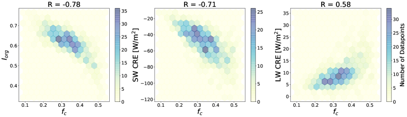
Figure S1: The 2D histograms of the relationships between $f_{c}$ and (a) $I_{org}$, (b) SWCRE, and (c) LWCRE with the reported Pearson’s correlation (R).

It is crucial to emphasize that the relationships illustrated in Fig. 1(a-c) are confounded by the variability of $f_{c}$, as $f_{c}$ is correlated with $I_{org}$, SWCRE, and LWCRE (Fig. S1). To eliminate the confounding effect of $f_{c}$, we employ the concept of partial correlation analysis Baba . (2004). For any given metric (e.g., $X$), we eliminate the variability associated with $f_{c}$ using a regression analysis,

$$X=c\times\text{$f_{c}$}+X|\text{$f_{c}$},$$ (1)

where $f_{c}$ serves as the regressor, $c$ represents the coefficient, and $X|\text{$f_{c}$}$ denotes the remaining variability in $X$ that cannot be explained by $f_{c}$.

Fig. 1(d) shows that as $I_{org}$$|$$f_{c}$ increases, SWCRE$|f_{c}$ becomes more negative, i.e., as clouds cluster, they reflect more incoming SW radiation. The resulting SW cooling amounts to up to 20 W/m² . This indicates that the positive correlation observed in Fig. 1(a) is due to $I_{org}$ and SWCRE being negatively correlated to $f_{c}$ (Fig. S1, a, b). Similarly, after elimination of $f_{c}$ variability, the response of LWCRE to cloud organization is strongly reduced to about 1 W/m² (Fig. 1, e), indicating that the correlation between $I_{org}$ and LWCRE in Fig. 1(b) is almost solely due to their mutual correlation with $f_{c}$ (Fig. S1, c). The variability in LWCRE due to clustering is thus similar in magnitude to the LW radiative effect ($\approx$ 0.75 W/m²) of the “cloud twilight zone” Eytan . (2020). Ultimately, as Fig. 1(f) illustrates, the dependence of net CRE on $I_{org}$$|$$f_{c}$ arises almost exclusively from the dependence of the SW component on cloud organization.

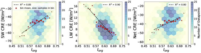
Figure 1: Dependence of domain-mean CRE on organization. In the first row (a-c), the relationships between $I_{org}$ and SWCRE (a), LWCRE (b), and net CRE (c) are illustrated. The second row (d-f) shows the same relationships but with removing the $f_{c}$ variability. The mean values of $I_{org}$ (for the $2^{nd}$ row, $I_{org}|f_{c}$) in each bin are denoted by red circles, with their size proportional to the number of points in the bin. The red dots are fitted with a dashed black line. Values below the $5^{th}$ and above the $95^{th}$ percentile of $I_{org}$ (for the $2^{nd}$ row, $I_{org}|f_{c}$) are excluded from the fit.

3.2 Clustering and cloud optical thickness are positively correlated

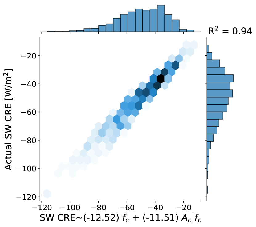
Figure S2: The result of the bi-linear regression analysis in which the target value is SWCRE and the regressors are $f_{c}$ and Ac$|$$f_{c}$ (Ac: cloud albedo observed by CERES). The reported coefficients are for the standardized $f_{c}$ and Ac$|$$f_{c}$. This plots ensures that the derived $f_{c}$ from MODIS cloud masks in addition to the observed albedo by CERES can significantly capture the variability in SWCRE.

In the previous section, we eliminated the impact of $f_{c}$ on the $I_{org}$-SWCRE relationship. The remaining variability in SWCRE is caused by variations in albedo and could be modulated by a sensitivity of 3D radiative effects to cloud organization. Regarding the latter, singer2021top report that biases in top-of-the-atmosphere SWCRE from neglecting 3D radiative effect are negligible for both, unorganized and organized shallow cumulus cloud fields (their Fig. 7). This is especially expected for averages over large domains, as analyzed here. Indeed, a bi-linear regression with $f_{c}$ and albedo as regressors can explain 94 % of variability in SWCRE in our dataset (Fig. S2). This confirms that the impact of 3D radiative effects is negligible in these large cloud fields.

Having 3D effects excluded, the remaining variability in SWCRE primarily corresponds to changes in albedo and equivalently cloud optical depth ${\tau}_{c}$. Figure 2(a) displays the variability of cloud patterns in a plane spanned by $\text{${\tau}_{c}$}|\text{$f_{c}$}$ and $\text{$I_{org}$}|\text{$f_{c}$}$. This figure shows a continuous range of patterns, in the terminology of stevens2020sugar ranging from Sugar and Gravels in the lower left corner to Fish and Flowers in the upper right corner.

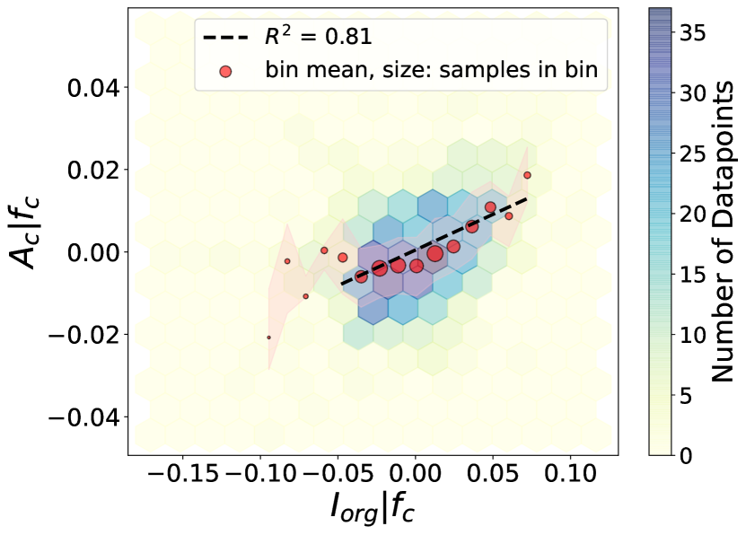
Figure S3: The relationship between $I_{org}$ and cloud albedo ($A_{c}$), having the effect of $f_{c}$ eliminated.

On average, $\text{${\tau}_{c}$}|\text{$f_{c}$}$ increases with increasing $\text{$I_{org}$}|\text{$f_{c}$}$ (Fig. 2, b). Despite the seemingly modest increase in $\text{${\tau}_{c}$}|\text{$f_{c}$}$, such changes can result in a significant increase in albedo of $0.03\text{ to }0.04$ (Figs. S3, S4), and the notable increase in SW reflection by 20 W/m² (Fig. 1, d). The $\text{$I_{org}$}|\text{$f_{c}$}$-$\text{${\tau}_{c}$}|\text{$f_{c}$}$ relationship indicates that horizontal cloud field organization, as measured by $I_{org}$, directly corresponds to its vertical organization, as captured by ${\tau}_{c}$: trade cumuli are optically thicker when they are more clustered.

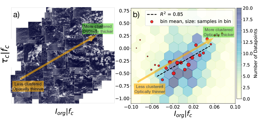
Figure 2: Dependence of domain-mean cloud optical depth on organization. The scatter plot of MODIS cloud features (a) and the 2-dimensional histogram (b) depict the $I_{org}$$|$$f_{c}$–${\tau}_{c}$$|$$f_{c}$ relationship. Specifically, for the scatter plot in (a), instead of displaying individual points, the entire cloud field is visualized to enhance pattern visualization. Clouds are represented in white, while the blue background represents the ocean color (MODIS true-color images). For plot (b), the mean values of $I_{org}|f_{c}$ in each bin are denoted by red circles, with their size proportional to the number of points in the bin. The red dots are fitted with a dashed black line. Values below the $5^{th}$ and above the $95^{th}$ percentile of $I_{org}|f_{c}$ are excluded from the fit.

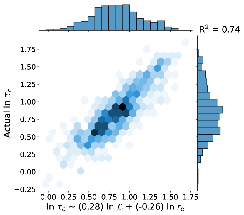
Figure S5: The result of the bi-linear regression analysis in which the target value is ln ${\tau}_{c}$ and the regressors are ln $\mathcal{L}$ and ln $r_{e}$. The reported coefficients are for the standardized ln $\mathcal{L}$ and ln $r_{e}$. This plots ensures that ln $\mathcal{L}$ and ln $r_{e}$ can significantly capture the variability in ln ${\tau}_{c}$, in line with theory.

As theoretically expected Han . (1994), ${\tau}_{c}$ is proportional to ${\text{$\mathcal{L}$}}/{\text{$r_{e}$}}$ in our dataset (Fig. S5). Figure 3 shows that both, $\mathcal{L}$ and $r_{e}$, contribute to mediating the relationship between organization and optical depth. With the $f_{c}$ effect eliminated, there is a positive correlation between the degree of cloud clustering and the amount of liquid water present within the clouds (Fig. 3, a). Similarly, as the level of clustering increases, clouds tend to exhibit smaller radii $r_{e}$ (Fig. 3, b). A cloud field that is dominated by Flowers shows smaller radii $r_{e}$ but higher liquid-water path $\mathcal{L}$ compared to the field dominated by Sugar and Gravels.

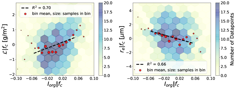
Figure 3: Dependence of domain-mean liquid water path and effective radius on organization. The figure shows the 2D histograms of the relationships between $I_{org}|f_{c}$ and $\mathcal{L}|f_{c}$ (a), and between $I_{org}|f_{c}$ and $r_{e}|f_{c}$ (b). The mean values of $I_{org}|f_{c}$ in each bin are denoted by red circles, with their size proportional to the number of points in the bin. The red dots are fitted with a dashed black line. Values below the $5^{th}$ and above the $95^{th}$ percentile of $I_{org}|f_{c}$ are excluded from the fit.

Our $\mathcal{L}$-organization relationship seems to be in contrast to schulz2021characterization who show that individual Gravel clouds have higher liquid-water path $\mathcal{L}$ compared to individual Flowers. To reconcile this with our results, we need to remind ourselves that the large cloud scenes analyzed here contain a mixture of different clouds. stevens2020sugar report that Gravel clouds tend to coexist with Sugar. For Flowers such a coexistence is less pronounced. Instead, Flowers feature anvils. Such shallow cumulus anvils have notable geometric thickness ($200$ m Wood . (2018) to 600 m Dauhut . (2023)). This means that anvil cloudiness is optically thicker and more reflective than typical Sugar (see also Fig. 7 in stevens2020sugar). When considering two cloud fields with identical $f_{c}$, it therefore seems reasonable that a Flower-dominated field features a larger domain-averaged $\mathcal{L}$ as compared to a field dominated by Sugar and Gravels.

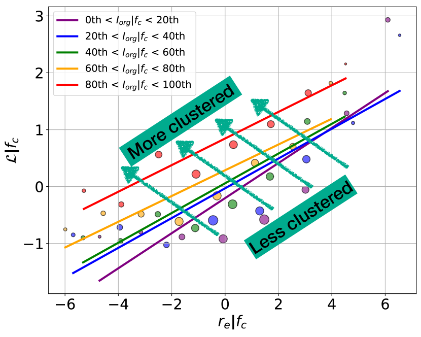
Figure S6: This figure highlights the positive correlation between $\mathcal{L}$ and $r_{e}$. However, when we examine the $\mathcal{L}$-$r_{e}$ relationship in relation to clustering, a clear pattern emerges: as clustering increases (more Flowers), $\mathcal{L}$ increases while $r_{e}$ decreases. Each distinct color in the figure represents a specific class of organization. For instance, the purple color represents cloud fields where the value of $I_{org}|f_{c}$ falls within the range of the 0th to 10th percentile of $I_{org}|f_{c}$.

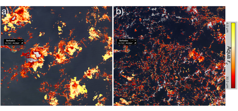
Figure S7: A Flowers (a) and a Gravel cloud field snapshots (from NASA Worldview) taken by Aqua satellites on 02/Feb/2020 and 17/Jan/2020, respectively. The cloud fields are colored by the value of $r_{e}$ which goes from 4 (yellow) to 30 (red) $\mu$m.

Similarly, the relationship between $I_{org}$, $\mathcal{L}$ and $r_{e}$ might seem unexpected: Based on adiabatic parcel lifting, we would expect $\mathcal{L}$ and $r_{e}$ to be positively correlated, while Fig. 3 suggests a negative correlation. In fact, $\mathcal{L}$ and $r_{e}$ are positively correlated in our dataset, while projecting their variability on organization ($I_{org}|f_{c}$) suggests a negative correlation: as degree of clustering increases, $\mathcal{L}$ increases but $r_{e}$ decreases (Fig. S6). Satellite snapshots of $r_{e}$ (Fig. S7) reveal that Flowers have substantially smaller $r_{e}$ in their veils compared to their core updrafts. In contrast, Gravels exhibit a more homogeneous $r_{e}$ with relatively larger values (compared to Flowers) associated with strong updrafts at the edge of their cold pool fronts. These observations suggest that for Flowers, the average $\mathcal{L}$ is primarily influenced by their cores, while the average $r_{e}$ is influenced by their veils. This is consistent with the fact that $\mathcal{L}$ is proportional to ${r_{e}}^{6}$, resulting in a more pronounced contrast between the core and veil in $\mathcal{L}$ compared to $r_{e}$. As a result, the average $\mathcal{L}$ of Flowers is larger compared to that of Gravels, while their average $r_{e}$ is smaller in comparison to Gravels.

It is interesting to contrast the small droplets in relatively thick anvils described here to the very large droplet sizes and optically thin veil clouds that have been reported in the context of the stratocumulus-to-cumulus transition Wood . (2018). While kuan2018deeper report an increase in the corresponding ultra-clean conditions with boundary layer height, this relationship is unlikely to extend to deep trade cumulus Flowers, which can be considered shallow mesoscale convective systems with complex outflow dynamics Dauhut . (2023). On the microphysical process level, ultra clean conditions have been associated with strong precipitation scavenging O, Wood  Bretherton (2018), while radtke2023spatial discuss that the conversion efficiency to precipitation decreases with increasing organization in trade cumulus.

Overall, our discussion of the relationship between liquid-water path and effective radius to organization and the resulting effects on optical depth highlight that organized cloud fields cannot be conceptualized with a single, typical profile of cloudiness. Instead, the spatial variability requires considering two types of clouds as discussed for Gravel and Sugar versus Flower cores and anvils. This duality resonates with the effective two-dimensionality of quantitative measures for mesoscale organization Janssens . (2021); Shamekh . (2023).

3.3 Mean cloud geometric thickness increases with clustering

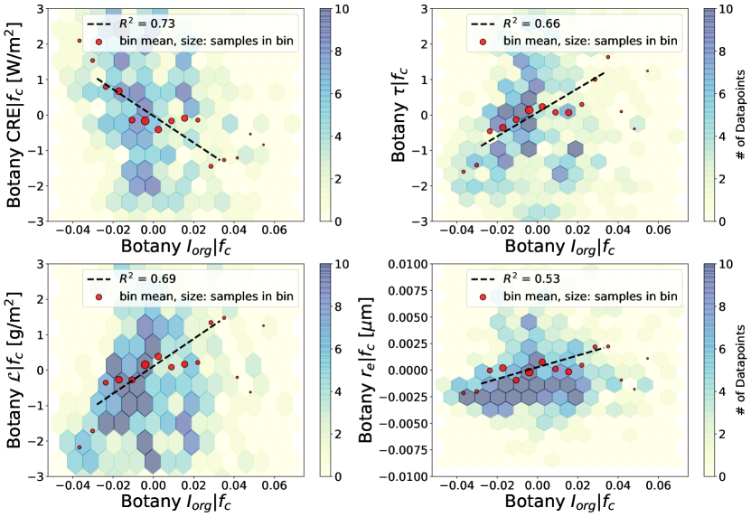
Figure S9: All results derived from the hourly analysis of the Cloud Botany dataset during the second day between the $37^{th}$ and $43^{rd}$ hours. Values below the $5^{th}$ and above the $95^{th}$ percentile of $I_{org}|f_{c}$ are excluded from the fitting.

For an entraining lifting parcel, liquid-water path $\mathcal{L}\propto f_{ad}h^{2}$, where $f_{ad}$ represents the degree of adiabaticity and $h$ denotes geometric cloud thickness. To explain the observed $I_{org}$-$\mathcal{L}$ relationship, we therefore investigate the relationships of $I_{org}$ to $h$ and $f_{ad}$ in the Botany simulations. Repeating the analysis from Sects. 3.1, 3.2 for the simulation data shows qualitative agreement and thus justifies this approach (Figs. S9(a-c), S10). Note that the discrepancy in the response of $r_{e}$ to cloud organization between simulations and satellite data (Fig. S9, d) is expected from the fixed cloud droplet number in the simulations but does not fundamentally affect our discussion of $\mathcal{L}$ here.

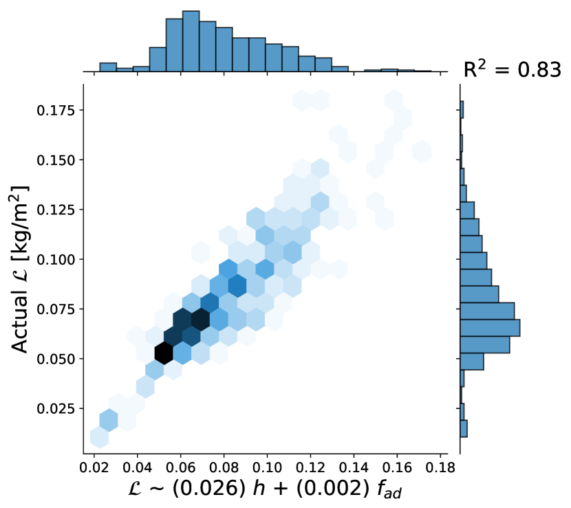
Figure S11: The result of the bi-linear regression analysis in which the target value is the in-cloud $\mathcal{L}$ and the regressors are $h$ and $f_{ad}$. The reported coefficients are for the standardized $h$ and $f_{ad}$.

Figure 4(a) shows that the domain-averaged geometric thickness increases by more than 100 m as cloud fields become more clustered (increasing $I_{org}|f_{c}$). Additionally, the variability in $h$ has a significantly larger influence on the value of $\mathcal{L}$ than $f_{ad}$ (Fig. S11). Thus, our LES-based results indicate that the simulated increase in $\mathcal{L}$ due to enhanced clustering (Fig. S9, c) primarily stems from the geometric thickening of cloud fields.

Figure 4(b) further explores the relationship between horizontal and vertical cloud field properties and shows that the average size of cloud objects ($L_{c}$) increases with $I_{org}|f_{c}$. This positive correlation shows that cloud horizontal extent as quantified by $L_{c}$, is positively correlated to cloud vertical extent as quantified by $h$, consistent with the findings of feingold2017analysis. The figure moreover illustrates that an increase in $I_{org}$$|$$f_{c}$ corresponds to a rise in the domain-average cloud-base height ($z_{b}$). Note that $z_{b}$ is not the lifting condensation level; instead, it represents the lowest height of a cloudy pixel within each column. This means that a higher domain-mean $z_{b}$ is an indication of the presence of more anvils in the field. Overall, Fig. 4(b) demonstrates that enhanced clustering leads to a higher occurrence of larger cloud objects with elevated domain-mean $z_{b}$, indicating a higher degree of anvilness.

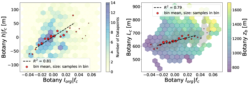
Figure 4: Dependence of domain-mean geometric thickness, average size of cloud objects, and domain-mean cloud-base height on organization. (a) The figure shows the 2D histogram of the relationship between $I_{org}|f_{c}$ and $h|f_{c}$. (b) The plot shows the relationship between $I_{org}|f_{c}$ and the mean-field cloud object size ($L_{c}$) with contour colors representing the values of domain-averaged cloud-base height ($z_{b}$). The gray shade indicates the inter-quartile range variability of $L_{c}$ in each bin of $I_{org}|f_{c}$. For both plots, the mean values of $I_{org}|f_{c}$ in each bin are denoted by red circles, with their size proportional to the number of points in the bin. The red dots are fitted with a dashed black line. For both plots, values below the $5^{th}$ and above the $95^{th}$ percentile of $I_{org}|f_{c}$ are excluded from the fit.

4 Conclusions & Outlook

We have explored the impact of shallow cumulus cloud field organization on cloud radiative effects, where confounding variability of $f_{c}$ was removed through partial correlation analysis (Eq. 1). Based on satellite data, our analysis shows that an increased level of clustering ($I_{org}|f_{c}$) results in up to 20 W/m² higher SW reflection to space (Fig. 1, d, f). We observe that, irrespective of $f_{c}$ variations, more clustered cloud fields exhibit, on average, higher liquid water path (Fig. 3, a), smaller cloud droplets (Fig. 3, b), and consequently, greater optical thickness (Fig. 2). A complementing ensemble of large-eddy simulations indicates that increased clustering leads to geometrically thicker cloud fields that feature increased anvilness (Fig. 4). Figure 5 summarizes these results. Collectively, they suggest that, eliminating the effect of $f_{c}$, the distribution of horizontal cloud sizes ultimately determines the vertical extent of clouds, subsequently influencing liquid-water path and cloud optical depth, and ultimately albedo and SWCRE.

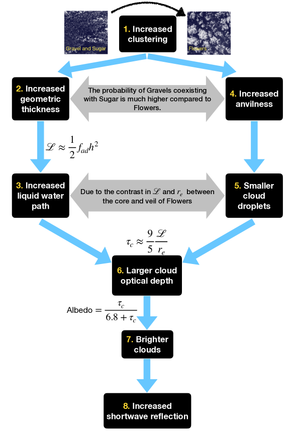
Figure 5: Summary of results. Comparing two cloud fields with identical cloud cover, the Flower-dominated cloud field features a larger domain-averaged geometric thickness, a higher liquid water path, more frequent anvils with smaller cloud droplets, and consequently, brighter clouds and therefore larger SW reflection in comparison to the cloud field dominated by the presence of Sugar and Gravels. In the diagram, theory-based equations are provided for arrows where the underlying theory exists. The gray arrows illustrate apparent paradoxes which are discussed in section 3.2.

What do our results mean in terms of the cloud feedback of trade cumulus? myers2021observational (their Supplementary Fig. 10) show that in addition to an increase in sea-surface temperature, which is not expected to trigger a notable response in trade cumulus cloudiness Myers . (2021); Cesana  Del Genio (2021), estimated inversion strength EIS is projected to moderately increase, and surface wind to slightly decrease. According to bony2020sugar such an increase in EIS would favor high-cloud-fraction Flowers over Gravel and Sugar with lower cloud fractions. In contrast, the decreasing surface wind would favor Sugar. While our results highlight the tight relationship between horizontal and vertical cloud organization, whether cloud fraction and optical depth interact positively or negatively in response to drivers of organization remains an open question. To address this interplay, we need to further explore how mesoscale processes Janssens . (2023); George . (2023); Vogel . (2021) modulate cloud fraction, liquid-water path, effective radii, and anvilness.

Data Availability

The cloud masks, provided by Aqua satellites, related to NASA’s MODIS instrument, can be extracted from level-1 Atmosphere Archive $\&$ Distribution System Distributed Active Archive Center (http://dx.doi.org/10.5067/MODIS/MYD06_L2.061). The data set related to CERES instrument is made available by Synoptic TOA and surface fluxes and clouds (SYN1deg - level 3) at https://ceres.larc.nasa.gov/data/#syn1deg-level-3. Prepossessing of cloud masks alongside calculation of organization metrics were done using the cloud metrics Gihub repository Denby  Janssens () available at https://github.com/cloudsci/cloudmetrics. The Botany dataset was downloaded using the EUREC⁴A intake catalog (https://howto.eurec4a.eu/botany_dales.html). The data was analyzed utilizing Python (used libraries: Numpy Harris . (2020), Pandas Wes McKinney (2010), Scipy Virtanen . (2020), Matplotlib Hunter (2007), and Seaborn Waskom (2021)). ChatGPT (OpenAI: https://openai.com/blog/chatgpt) has been used for copy-editing during the preparation of the manuscript.

Supplementary Information for “Shallow Cumulus Cloud Fields Are Optically Thicker When They Are More Clustered”

This file includes some additional figures for supporting the main text of our paper (First part). Additionally, the detailed calculation of adiabaticity is presented (Second part).

Supplementary Figures

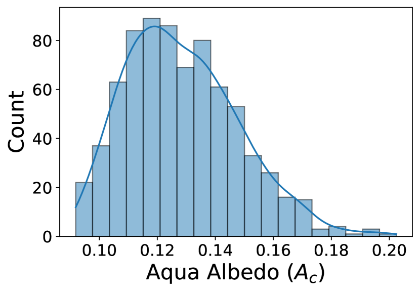
Figure S4: The histogram plot of cloud scene albedo ($A_{c}$) in the Aqua satellite dataset. This plot shows that the range of variability in cloud field albedo is about 0.1.

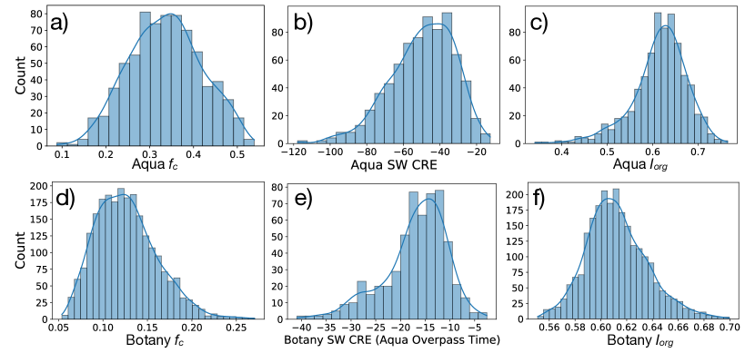
Figure S8: Histograms of $f_{c}$, SWCRE and $I_{org}$ for Aqua (a,b,c) and Botany (d,e,f) datasets, respectively. The values of SWCRE are in W/m². Note that the histograms of $f_{c}$ and $I_{org}$ are for the whole Botany dataset, while the Botany’s SWCRE is only for hours 37-43 (day-time values).

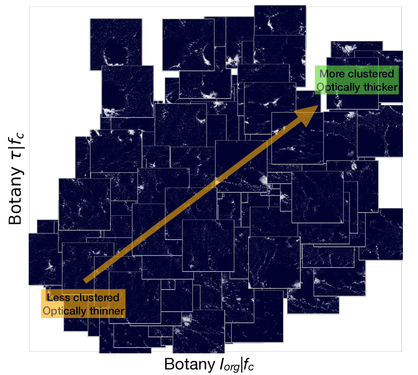
Figure S10: Similar to Fig. 2(a) but for the Botany dataset during hours 37-43.

Calculation of the degree of adiabaticity

The degree of adiabaticity is computed using the following equation:

$$f_{ad}=\dfrac{\int_{z_{b}}^{z_{t}}\rho(z)q_{l}(z)dz}{\int_{z_{b}}^{z_{t}}\rho(z)\Gamma_{ad}(z)zdz}$$ (2)

where, $z$ represents the height, $\rho(z)$, $q_{l}(z)$, and $\Gamma_{ad}(z)$ denotes density, liquid water specific humidity, and the moist adiabatic lapse rate of $q_{l}$ at each model height. To ensure a more precise estimation, $f_{ad}$ is computed only for columns where the associated $z_{b}$ is in proximity to the lifting condensation level ($<$850 m) and the cloud thickness exceeds 150 m.

The calculation of $\Gamma_{ad}$ is determined by the following equation Schmeissner . (2015); Eytan . (2021):

$$\Gamma_{ad}=\frac{c_{p}}{L_{v}}\left(\Gamma_{m}+\frac{g}{c_{p}}\right)$$ (3)

Here, $c_{p}$ represents the specific heat constant, $g$ denotes the acceleration due to gravity, $L_{v}$ stands for the latent heat of vaporization. The moist adiabatic lapse rate for temperature, $\Gamma_{m}$, is computed as:

$$\Gamma_{m}=\dfrac{g}{c_{p}}\left(\dfrac{1+\dfrac{L_{v}}{R_{d}T}q_{s}}{1+\dfrac{\beta L_{v}}{c_{p}}q_{s}}\right)$$ (4)

In the above equation, $R_{d}$ corresponds to the gas constant for dry air, $T$ represents temperature, $\beta$ is the constant in the Clausius-Clapeyron equation ($e_{s}=A\exp(\beta(T-T_{0}))$), and $q_{s}$ denotes the saturation specific humidity, which can be approximated as $\approx 0.622\frac{{e_{s}}}{{P}}$ where $P$ represents pressure.

For simplicity, we calculate $\Gamma_{ad}$ for the middle of the cloud layer (at $z^{\prime}=\dfrac{z_{b}+z_{t}}{2}$) and assume that it linearly changes with height through the cloud layer. This assumption leads to the equation below:

$$f_{ad}=\dfrac{\int_{z_{b}}^{z_{t}}\rho(z)q_{l}(z)dz}{\Gamma_{ad}(z^{\prime})\int_{z_{b}}^{z_{t}}\rho(z)zdz}$$ (5)

where, a $f_{ad}$ value of 1 in each column indicates a fully adiabatic cloud, while values smaller than 1 and larger than 0 indicate non-adiabatic clouds. In the final step, after obtaining $f_{ad}$ for each column, we proceed to calculate the domain-mean $f_{ad}$ for the entire cloud field.

References

- Baba \BOthers. (\APACyear2004) \APACinsertmetastarbaba2004partial{APACrefauthors}Baba, K., Shibata, R.\BCBL \BBA Sibuya, M. \APACrefYearMonthDay2004. \BBOQ\APACrefatitlePartial correlation and conditional correlation as measures of conditional independence Partial correlation and conditional correlation as measures of conditional independence.\BBCQ \APACjournalVolNumPagesAustralian & New Zealand Journal of Statistics464657–664. {APACrefDOI} \doi10.1111/j.1467-842X.2004.00360.x \PrintBackRefs\CurrentBib
- Bony \BBA Dufresne (\APACyear2005) \APACinsertmetastarbony2005marine{APACrefauthors}Bony, S.\BCBT \BBA Dufresne, J\BHBIL. \APACrefYearMonthDay2005. \BBOQ\APACrefatitleMarine boundary layer clouds at the heart of tropical cloud feedback uncertainties in climate models Marine boundary layer clouds at the heart of tropical cloud feedback uncertainties in climate models.\BBCQ \APACjournalVolNumPagesGeophysical Research Letters3220. {APACrefDOI} \doi10.1029/2005GL023851 \PrintBackRefs\CurrentBib
- Bony \BOthers. (\APACyear2004) \APACinsertmetastarbony2004dynamic{APACrefauthors}Bony, S., Dufresne, J\BHBIL., Le Treut, H., Morcrette, J\BHBIJ.\BCBL \BBA Senior, C. \APACrefYearMonthDay2004. \BBOQ\APACrefatitleOn dynamic and thermodynamic components of cloud changes On dynamic and thermodynamic components of cloud changes.\BBCQ \APACjournalVolNumPagesClimate Dynamics22271–86. {APACrefDOI} \doi10.1007/s00382-003-0369-6 \PrintBackRefs\CurrentBib
- Bony \BOthers. (\APACyear2020) \APACinsertmetastarbony2020sugar{APACrefauthors}Bony, S., Schulz, H., Vial, J.\BCBL \BBA Stevens, B. \APACrefYearMonthDay2020. \BBOQ\APACrefatitleSugar, gravel, fish, and flowers: Dependence of mesoscale patterns of trade-wind clouds on environmental conditions Sugar, gravel, fish, and flowers: Dependence of mesoscale patterns of trade-wind clouds on environmental conditions.\BBCQ \APACjournalVolNumPagesGeophysical Research Letters477e2019GL085988. {APACrefDOI} \doi10.1029/2019GL085988 \PrintBackRefs\CurrentBib
- Bony \BOthers. (\APACyear2015) \APACinsertmetastarbony2015clouds{APACrefauthors}Bony, S., Stevens, B., Frierson, D\BPBIM., Jakob, C., Kageyama, M., Pincus, R.\BDBLothers \APACrefYearMonthDay2015. \BBOQ\APACrefatitleClouds, circulation and climate sensitivity Clouds, circulation and climate sensitivity.\BBCQ \APACjournalVolNumPagesNature Geoscience84261–268. {APACrefDOI} \doi10.1038/ngeo2398 \PrintBackRefs\CurrentBib
- Cesana \BBA Del Genio (\APACyear2021) \APACinsertmetastarcesana2021observational{APACrefauthors}Cesana, G\BPBIV.\BCBT \BBA Del Genio, A\BPBID. \APACrefYearMonthDay2021. \BBOQ\APACrefatitleObservational constraint on cloud feedbacks suggests moderate climate sensitivity Observational constraint on cloud feedbacks suggests moderate climate sensitivity.\BBCQ \APACjournalVolNumPagesNature Climate Change113213–218. {APACrefDOI} \doi10.1038/s41558-020-00970-y \PrintBackRefs\CurrentBib
- Dauhut \BOthers. (\APACyear2023) \APACinsertmetastardauhut2023flower{APACrefauthors}Dauhut, T., Couvreux, F., Bouniol, D., Beucher, F., Volkmer, L., Pörtge, V.\BDBLothers \APACrefYearMonthDay2023. \BBOQ\APACrefatitleFlower trade-wind clouds are shallow mesoscale convective systems Flower trade-wind clouds are shallow mesoscale convective systems.\BBCQ \APACjournalVolNumPagesQuarterly Journal of the Royal Meteorological Society149750325–347. {APACrefDOI} \doi10.1002/qj.4409 \PrintBackRefs\CurrentBib
- Denby (\APACyear2020) \APACinsertmetastardenby2020discovering{APACrefauthors}Denby, L. \APACrefYearMonthDay2020. \BBOQ\APACrefatitleDiscovering the importance of mesoscale cloud organization through unsupervised classification Discovering the importance of mesoscale cloud organization through unsupervised classification.\BBCQ \APACjournalVolNumPagesGeophysical Research Letters471e2019GL085190. {APACrefDOI} \doi10.1029/2019GL085190 \PrintBackRefs\CurrentBib
- Denby (\APACyear2023) \APACinsertmetastardenby2023charting{APACrefauthors}Denby, L. \APACrefYearMonthDay2023. \APACrefbtitleCharting the Realms of Mesoscale Cloud Organisation using Unsupervised Learning. Charting the realms of mesoscale cloud organisation using unsupervised learning. {APACrefDOI} \doihttps://doi.org/10.48550/arXiv.2309.08567 \PrintBackRefs\CurrentBib
- Denby \BBA Janssens (\APACyear\bibnodate) \APACinsertmetastarDenby_cloudmetrics{APACrefauthors}Denby, L.\BCBT \BBA Janssens, M. \APACrefYearMonthDay\bibnodate. \APACrefbtitlecloudmetrics. cloudmetrics. \PrintBackRefs\CurrentBib
- Eytan \BOthers. (\APACyear2020) \APACinsertmetastareytan2020longwave{APACrefauthors}Eytan, E., Koren, I., Altaratz, O., Kostinski, A\BPBIB.\BCBL \BBA Ronen, A. \APACrefYearMonthDay2020. \BBOQ\APACrefatitleLongwave radiative effect of the cloud twilight zone Longwave radiative effect of the cloud twilight zone.\BBCQ \APACjournalVolNumPagesNature Geoscience1310669–673. {APACrefDOI} \doi10.1038/s41561-020-0636-8 \PrintBackRefs\CurrentBib
- Eytan \BOthers. (\APACyear2021) \APACinsertmetastareytan2021revisiting{APACrefauthors}Eytan, E., Koren, I., Altaratz, O., Pinsky, M.\BCBL \BBA Khain, A. \APACrefYearMonthDay2021. \BBOQ\APACrefatitleRevisiting adiabatic fraction estimations in cumulus clouds: high-resolution simulations with a passive tracer Revisiting adiabatic fraction estimations in cumulus clouds: high-resolution simulations with a passive tracer.\BBCQ \APACjournalVolNumPagesAtmospheric Chemistry and Physics212116203–16217. {APACrefDOI} \doi10.5194/acp-21-16203-2021 \PrintBackRefs\CurrentBib
- Feingold \BOthers. (\APACyear2017) \APACinsertmetastarfeingold2017analysis{APACrefauthors}Feingold, G., Balsells, J., Glassmeier, F., Yamaguchi, T., Kazil, J.\BCBL \BBA McComiskey, A. \APACrefYearMonthDay2017. \BBOQ\APACrefatitleAnalysis of albedo versus cloud fraction relationships in liquid water clouds using heuristic models and large eddy simulation Analysis of albedo versus cloud fraction relationships in liquid water clouds using heuristic models and large eddy simulation.\BBCQ \APACjournalVolNumPagesJournal of Geophysical Research: Atmospheres122137086–7102. {APACrefDOI} \doi10.1002/2017JD026467 \PrintBackRefs\CurrentBib
- George \BOthers. (\APACyear2023) \APACinsertmetastargeorge2023widespread{APACrefauthors}George, G., Stevens, B., Bony, S., Vogel, R.\BCBL \BBA Naumann, A\BPBIK. \APACrefYearMonthDay2023. \BBOQ\APACrefatitleWidespread shallow mesoscale circulations observed in the trades Widespread shallow mesoscale circulations observed in the trades.\BBCQ \APACjournalVolNumPagesNature Geoscience1–6. {APACrefDOI} \doi10.1038/s41561-023-01215-1 \PrintBackRefs\CurrentBib
- Han \BOthers. (\APACyear1994) \APACinsertmetastarhan1994near{APACrefauthors}Han, Q., Rossow, W\BPBIB.\BCBL \BBA Lacis, A\BPBIA. \APACrefYearMonthDay1994. \BBOQ\APACrefatitleNear-global survey of effective droplet radii in liquid water clouds using ISCCP data Near-global survey of effective droplet radii in liquid water clouds using isccp data.\BBCQ \APACjournalVolNumPagesJournal of Climate74465–497. {APACrefDOI} \doi10.1175/1520-0442(1994)007¡0465:NGSOED¿2.0.CO;2 \PrintBackRefs\CurrentBib
- Harris \BOthers. (\APACyear2020) \APACinsertmetastarharris2020array{APACrefauthors}Harris, C\BPBIR., Millman, K\BPBIJ., van der Walt, S\BPBIJ., Gommers, R., Virtanen, P., Cournapeau, D.\BDBLOliphant, T\BPBIE. \APACrefYearMonthDay2020\APACmonth09. \BBOQ\APACrefatitleArray programming with NumPy Array programming with NumPy.\BBCQ \APACjournalVolNumPagesNature5857825357–362. {APACrefURL} https://doi.org/10.1038/s41586-020-2649-2 {APACrefDOI} \doi10.1038/s41586-020-2649-2 \PrintBackRefs\CurrentBib
- Hersbach \BOthers. (\APACyear2020) \APACinsertmetastarhersbach2020era5{APACrefauthors}Hersbach, H., Bell, B., Berrisford, P., Hirahara, S., Horányi, A., Muñoz-Sabater, J.\BDBLothers \APACrefYearMonthDay2020. \BBOQ\APACrefatitleThe ERA5 global reanalysis The ERA5 global reanalysis.\BBCQ \APACjournalVolNumPagesQuarterly Journal of the Royal Meteorological Society1467301999–2049. {APACrefDOI} \doi10.1002/qj.3803 \PrintBackRefs\CurrentBib
- Hunter (\APACyear2007) \APACinsertmetastarHunter:2007{APACrefauthors}Hunter, J\BPBID. \APACrefYearMonthDay2007. \BBOQ\APACrefatitleMatplotlib: A 2D graphics environment Matplotlib: A 2D graphics environment.\BBCQ \APACjournalVolNumPagesComputing in Science & Engineering9390–95. {APACrefDOI} \doi10.1109/MCSE.2007.55 \PrintBackRefs\CurrentBib
- Janssens \BOthers. (\APACyear2023) \APACinsertmetastarjanssens2023nonprecipitating{APACrefauthors}Janssens, M., de Arellano, J\BPBIV\BHBIG., van Heerwaarden, C\BPBIC., de Roode, S\BPBIR., Siebesma, A\BPBIP.\BCBL \BBA Glassmeier, F. \APACrefYearMonthDay2023. \BBOQ\APACrefatitleNonprecipitating Shallow Cumulus Convection Is Intrinsically Unstable to Length Scale Growth Nonprecipitating shallow cumulus convection is intrinsically unstable to length scale growth.\BBCQ \APACjournalVolNumPagesJournal of the Atmospheric Sciences803849–870. {APACrefDOI} \doi10.1175/JAS-D-22-0111.1 \PrintBackRefs\CurrentBib
- Janssens \BOthers. (\APACyear2021) \APACinsertmetastarjanssens2021cloud{APACrefauthors}Janssens, M., Vilà-Guerau de Arellano, J., Scheffer, M., Antonissen, C., Siebesma, A\BPBIP.\BCBL \BBA Glassmeier, F. \APACrefYearMonthDay2021. \BBOQ\APACrefatitleCloud patterns in the trades have four interpretable dimensions Cloud patterns in the trades have four interpretable dimensions.\BBCQ \APACjournalVolNumPagesGeophysical Research Letters485e2020GL091001. {APACrefDOI} \doi10.1029/2020GL091001 \PrintBackRefs\CurrentBib
- Jansson \BOthers. (\APACyear2023) \APACinsertmetastarjansson2023cloud{APACrefauthors}Jansson, F., Janssens, M., Grönqvist, J\BPBIH., Siebesma, P., Glassmeier, F., Attema, J\BPBIJ.\BDBLothers \APACrefYearMonthDay2023. \BBOQ\APACrefatitleCloud Botany: Shallow cumulus clouds in an ensemble of idealized large-domain large-eddy simulations of the trades Cloud botany: Shallow cumulus clouds in an ensemble of idealized large-domain large-eddy simulations of the trades.\BBCQ \APACjournalVolNumPagessubmitted to Journal of Advances in Modeling Earth Systems, preprint: https://www.authorea.com/doi/full/10.22541/essoar.168319841.11427814. {APACrefDOI} \doi10.22541/essoar.168319841.11427814/v1 \PrintBackRefs\CurrentBib
- Johnson \BOthers. (\APACyear1999) \APACinsertmetastarjohnson1999trimodal{APACrefauthors}Johnson, R\BPBIH., Rickenbach, T\BPBIM., Rutledge, S\BPBIA., Ciesielski, P\BPBIE.\BCBL \BBA Schubert, W\BPBIH. \APACrefYearMonthDay1999. \BBOQ\APACrefatitleTrimodal characteristics of tropical convection Trimodal characteristics of tropical convection.\BBCQ \APACjournalVolNumPagesJournal of climate1282397–2418. {APACrefDOI} \doi10.1175/1520-0442(1999)012¡2397:TCOTC¿2.0.CO;2 \PrintBackRefs\CurrentBib
- Luebke \BOthers. (\APACyear2022) \APACinsertmetastarluebke2022assessment{APACrefauthors}Luebke, A\BPBIE., Ehrlich, A., Schäfer, M., Wolf, K.\BCBL \BBA Wendisch, M. \APACrefYearMonthDay2022. \BBOQ\APACrefatitleAn assessment of macrophysical and microphysical cloud properties driving radiative forcing of shallow trade-wind clouds An assessment of macrophysical and microphysical cloud properties driving radiative forcing of shallow trade-wind clouds.\BBCQ \APACjournalVolNumPagesAtmospheric Chemistry and Physics2242727–2744. {APACrefDOI} \doi10.5194/acp-22-2727-2022 \PrintBackRefs\CurrentBib
- McCoy \BOthers. (\APACyear2022) \APACinsertmetastarmccoy2022role{APACrefauthors}McCoy, I\BPBIL., McCoy, D\BPBIT., Wood, R., Zuidema, P.\BCBL \BBA Bender, F\BPBIA\BHBIM. \APACrefYearMonthDay2022. \BBOQ\APACrefatitleThe Role of Mesoscale Cloud Morphology in the Shortwave Cloud Feedback The role of mesoscale cloud morphology in the shortwave cloud feedback.\BBCQ \APACjournalVolNumPagesGeophysical Research Letterse2022GL101042. {APACrefDOI} \doi10.1029/2022GL101042 \PrintBackRefs\CurrentBib
- Medeiros \BBA Nuijens (\APACyear2016) \APACinsertmetastarmedeiros2016clouds{APACrefauthors}Medeiros, B.\BCBT \BBA Nuijens, L. \APACrefYearMonthDay2016. \BBOQ\APACrefatitleClouds at Barbados are representative of clouds across the trade wind regions in observations and climate models Clouds at Barbados are representative of clouds across the trade wind regions in observations and climate models.\BBCQ \APACjournalVolNumPagesProceedings of the National Academy of Sciences11322E3062–E3070. {APACrefDOI} \doi10.1073/pnas.1521494113 \PrintBackRefs\CurrentBib
- Myers \BOthers. (\APACyear2021) \APACinsertmetastarmyers2021observational{APACrefauthors}Myers, T\BPBIA., Scott, R\BPBIC., Zelinka, M\BPBID., Klein, S\BPBIA., Norris, J\BPBIR.\BCBL \BBA Caldwell, P\BPBIM. \APACrefYearMonthDay2021. \BBOQ\APACrefatitleObservational constraints on low cloud feedback reduce uncertainty of climate sensitivity Observational constraints on low cloud feedback reduce uncertainty of climate sensitivity.\BBCQ \APACjournalVolNumPagesNature Climate Change116501–507. {APACrefDOI} \doi10.1038/s41558-021-01039-0 \PrintBackRefs\CurrentBib
- Nuijens \BBA Siebesma (\APACyear2019) \APACinsertmetastarnuijens2019boundary{APACrefauthors}Nuijens, L.\BCBT \BBA Siebesma, A\BPBIP. \APACrefYearMonthDay2019. \BBOQ\APACrefatitleBoundary layer clouds and convection over subtropical oceans in our current and in a warmer climate Boundary layer clouds and convection over subtropical oceans in our current and in a warmer climate.\BBCQ \APACjournalVolNumPagesCurrent Climate Change Reports5280–94. {APACrefDOI} \doi10.1007/s40641-019-00126-x \PrintBackRefs\CurrentBib
- O, Wood\BCBL \BBA Bretherton (\APACyear2018) \APACinsertmetastarkuan2018ultraclean{APACrefauthors}O, K\BHBIT., Wood, R.\BCBL \BBA Bretherton, C\BPBIS. \APACrefYearMonthDay2018. \BBOQ\APACrefatitleUltraclean layers and optically thin clouds in the stratocumulus-to-cumulus transition. Part II: Depletion of cloud droplets and cloud condensation nuclei through collision–coalescence Ultraclean layers and optically thin clouds in the stratocumulus-to-cumulus transition. Part II: Depletion of cloud droplets and cloud condensation nuclei through collision–coalescence.\BBCQ \APACjournalVolNumPagesJournal of the Atmospheric Sciences7551653–1673. {APACrefDOI} \doi10.1175/JAS-D-17-0218.1 \PrintBackRefs\CurrentBib
- O, Wood, Tseng\BCBL \BOthers. (\APACyear2018) \APACinsertmetastarkuan2018deeper{APACrefauthors}O, K\BHBIT., Wood, R., Tseng, H.\BCBL \BOthersPeriod. \APACrefYearMonthDay2018. \BBOQ\APACrefatitleDeeper, precipitating PBLs associated with optically thin veil clouds in the Sc-Cu transition. Deeper, precipitating PBLs associated with optically thin veil clouds in the Sc-Cu transition.\BBCQ \APACjournalVolNumPagesGeophysical Research Letters45105177–5184. {APACrefDOI} \doi10.1029/2018GL077084 \PrintBackRefs\CurrentBib
- Painemal \BBA Zuidema (\APACyear2011) \APACinsertmetastarpainemal2011assessment{APACrefauthors}Painemal, D.\BCBT \BBA Zuidema, P. \APACrefYearMonthDay2011. \BBOQ\APACrefatitleAssessment of MODIS cloud effective radius and optical thickness retrievals over the Southeast Pacific with VOCALS-REX in situ measurements Assessment of MODIS cloud effective radius and optical thickness retrievals over the southeast pacific with VOCALS-REX in situ measurements.\BBCQ \APACjournalVolNumPagesJournal of Geophysical Research: Atmospheres116D24. {APACrefDOI} \doi10.1029/2011JD016155 \PrintBackRefs\CurrentBib
- Radtke \BOthers. (\APACyear2023) \APACinsertmetastarradtke2023spatial{APACrefauthors}Radtke, J., Vogel, R., Ament, F.\BCBL \BBA Naumann, A\BPBIK. \APACrefYearMonthDay2023. \BBOQ\APACrefatitleSpatial organisation affects the pathway to precipitation in simulated trade-wind convection Spatial organisation affects the pathway to precipitation in simulated trade-wind convection.\BBCQ \APACjournalVolNumPagesSubmitted to Geophysical Research Letters, preprint: https://www.authorea.com/doi/full/10.22541/essoar.167979635.58663858. {APACrefDOI} \doi10.22541/essoar.167979635.58663858/v2 \PrintBackRefs\CurrentBib
- Schmeissner \BOthers. (\APACyear2015) \APACinsertmetastarschmeissner2015turbulent{APACrefauthors}Schmeissner, T., Shaw, R., Ditas, J., Stratmann, F., Wendisch, M.\BCBL \BBA Siebert, H. \APACrefYearMonthDay2015. \BBOQ\APACrefatitleTurbulent mixing in shallow trade wind cumuli: Dependence on cloud life cycle Turbulent mixing in shallow trade wind cumuli: Dependence on cloud life cycle.\BBCQ \APACjournalVolNumPagesJournal of the Atmospheric Sciences7241447–1465. {APACrefDOI} \doi10.1175/JAS-D-14-0230.1 \PrintBackRefs\CurrentBib
- Schneider \BOthers. (\APACyear2017) \APACinsertmetastarschneider2017climate{APACrefauthors}Schneider, T., Teixeira, J., Bretherton, C\BPBIS., Brient, F., Pressel, K\BPBIG., Schär, C.\BCBL \BBA Siebesma, A\BPBIP. \APACrefYearMonthDay2017. \BBOQ\APACrefatitleClimate goals and computing the future of clouds Climate goals and computing the future of clouds.\BBCQ \APACjournalVolNumPagesNature Climate Change713–5. {APACrefDOI} \doi10.1038/nclimate3190 \PrintBackRefs\CurrentBib
- Schulz \BOthers. (\APACyear2021) \APACinsertmetastarschulz2021characterization{APACrefauthors}Schulz, H., Eastman, R.\BCBL \BBA Stevens, B. \APACrefYearMonthDay2021. \BBOQ\APACrefatitleCharacterization and evolution of organized shallow convection in the trades Characterization and evolution of organized shallow convection in the trades.\BBCQ \APACjournalVolNumPagesJournal of Geophysical Research: Atmospheres. {APACrefDOI} \doi10.1029/2021JD034575 \PrintBackRefs\CurrentBib
- Seethala \BBA Horváth (\APACyear2010) \APACinsertmetastarseethala2010global{APACrefauthors}Seethala, C.\BCBT \BBA Horváth, Á. \APACrefYearMonthDay2010. \BBOQ\APACrefatitleGlobal assessment of AMSR-E and MODIS cloud liquid water path retrievals in warm oceanic clouds Global assessment of AMSR-E and MODIS cloud liquid water path retrievals in warm oceanic clouds.\BBCQ \APACjournalVolNumPagesJournal of Geophysical Research: Atmospheres115D13. {APACrefDOI} \doi10.1029/2009JD012662 \PrintBackRefs\CurrentBib
- Shamekh \BOthers. (\APACyear2023) \APACinsertmetastarshamekh2023implicit{APACrefauthors}Shamekh, S., Lamb, K\BPBID., Huang, Y.\BCBL \BBA Gentine, P. \APACrefYearMonthDay2023. \BBOQ\APACrefatitleImplicit learning of convective organization explains precipitation stochasticity Implicit learning of convective organization explains precipitation stochasticity.\BBCQ \APACjournalVolNumPagesProceedings of the National Academy of Sciences12020e2216158120. {APACrefDOI} \doi10.1073/pnas.2216158120 \PrintBackRefs\CurrentBib
- Sherwood \BOthers. (\APACyear2020) \APACinsertmetastarsherwood2020assessment{APACrefauthors}Sherwood, S\BPBIC., Webb, M\BPBIJ., Annan, J\BPBID., Armour, K\BPBIC., Forster, P\BPBIM., Hargreaves, J\BPBIC.\BDBLothers \APACrefYearMonthDay2020. \BBOQ\APACrefatitleAn assessment of Earth’s climate sensitivity using multiple lines of evidence An assessment of Earth’s climate sensitivity using multiple lines of evidence.\BBCQ \APACjournalVolNumPagesReviews of Geophysics584e2019RG000678. {APACrefDOI} \doi10.1029/2019RG000678 \PrintBackRefs\CurrentBib
- Singer \BOthers. (\APACyear2021) \APACinsertmetastarsinger2021top{APACrefauthors}Singer, C\BPBIE., Lopez-Gomez, I., Zhang, X.\BCBL \BBA Schneider, T. \APACrefYearMonthDay2021. \BBOQ\APACrefatitleTop-of-atmosphere albedo bias from neglecting three-dimensional cloud radiative effects Top-of-atmosphere albedo bias from neglecting three-dimensional cloud radiative effects.\BBCQ \APACjournalVolNumPagesJournal of the Atmospheric Sciences78124053–4069. {APACrefDOI} \doi10.1175/JAS-D-21-0032.1 \PrintBackRefs\CurrentBib
- Stevens \BOthers. (\APACyear2020) \APACinsertmetastarstevens2020sugar{APACrefauthors}Stevens, B., Bony, S., Brogniez, H., Hentgen, L., Hohenegger, C., Kiemle, C.\BDBLothers \APACrefYearMonthDay2020. \BBOQ\APACrefatitleSugar, gravel, fish and flowers: Mesoscale cloud patterns in the trade winds Sugar, gravel, fish and flowers: Mesoscale cloud patterns in the trade winds.\BBCQ \APACjournalVolNumPagesQuarterly Journal of the Royal Meteorological Society146726141–152. {APACrefDOI} \doi10.1002/qj.3662 \PrintBackRefs\CurrentBib
- Tobin \BOthers. (\APACyear2012) \APACinsertmetastartobin2012observational{APACrefauthors}Tobin, I., Bony, S.\BCBL \BBA Roca, R. \APACrefYearMonthDay2012. \BBOQ\APACrefatitleObservational evidence for relationships between the degree of aggregation of deep convection, water vapor, surface fluxes, and radiation Observational evidence for relationships between the degree of aggregation of deep convection, water vapor, surface fluxes, and radiation.\BBCQ \APACjournalVolNumPagesJournal of Climate25206885–6904. {APACrefDOI} \doi10.1175/JCLI-D-11-00258.1 \PrintBackRefs\CurrentBib
- Tompkins \BBA Semie (\APACyear2017) \APACinsertmetastartompkins2017organization{APACrefauthors}Tompkins, A\BPBIM.\BCBT \BBA Semie, A\BPBIG. \APACrefYearMonthDay2017. \BBOQ\APACrefatitleOrganization of tropical convection in low vertical wind shears: Role of updraft entrainment Organization of tropical convection in low vertical wind shears: Role of updraft entrainment.\BBCQ \APACjournalVolNumPagesJournal of Advances in Modeling Earth Systems921046–1068. {APACrefDOI} \doi10.1002/2016MS000802 \PrintBackRefs\CurrentBib
- Virtanen \BOthers. (\APACyear2020) \APACinsertmetastar2020SciPy-NMeth{APACrefauthors}Virtanen, P., Gommers, R., Oliphant, T\BPBIE., Haberland, M., Reddy, T., Cournapeau, D.\BDBLSciPy 1.0 Contributors \APACrefYearMonthDay2020. \BBOQ\APACrefatitleSciPy 1.0: Fundamental Algorithms for Scientific Computing in Python SciPy 1.0: Fundamental Algorithms for Scientific Computing in Python.\BBCQ \APACjournalVolNumPagesNature Methods17261–272. {APACrefDOI} \doi10.1038/s41592-019-0686-2 \PrintBackRefs\CurrentBib
- Vogel \BOthers. (\APACyear2022) \APACinsertmetastarvogel2022strong{APACrefauthors}Vogel, R., Albright, A\BPBIL., Vial, J., George, G., Stevens, B.\BCBL \BBA Bony, S. \APACrefYearMonthDay2022. \BBOQ\APACrefatitleStrong cloud–circulation coupling explains weak trade cumulus feedback Strong cloud–circulation coupling explains weak trade cumulus feedback.\BBCQ \APACjournalVolNumPagesNature1–5. {APACrefDOI} \doi10.1038/s41586-022-05364-y \PrintBackRefs\CurrentBib
- Vogel \BOthers. (\APACyear2021) \APACinsertmetastarvogel2021climatology{APACrefauthors}Vogel, R., Konow, H., Schulz, H.\BCBL \BBA Zuidema, P. \APACrefYearMonthDay2021. \BBOQ\APACrefatitleA climatology of trade-wind cumulus cold pools and their link to mesoscale cloud organization A climatology of trade-wind cumulus cold pools and their link to mesoscale cloud organization.\BBCQ \APACjournalVolNumPagesAtmospheric Chemistry and Physics212116609–16630. {APACrefDOI} \doi10.5194/acp-21-16609-2021 \PrintBackRefs\CurrentBib
- Waskom (\APACyear2021) \APACinsertmetastarWaskom2021{APACrefauthors}Waskom, M\BPBIL. \APACrefYearMonthDay2021. \BBOQ\APACrefatitleseaborn: statistical data visualization seaborn: statistical data visualization.\BBCQ \APACjournalVolNumPagesJournal of Open Source Software6603021. {APACrefURL} https://doi.org/10.21105/joss.03021 {APACrefDOI} \doi10.21105/joss.03021 \PrintBackRefs\CurrentBib
- Weger \BOthers. (\APACyear1992) \APACinsertmetastarweger1992clustering{APACrefauthors}Weger, R., Lee, J., Zhu, T.\BCBL \BBA Welch, R. \APACrefYearMonthDay1992. \BBOQ\APACrefatitleClustering, randomness and regularity in cloud fields: 1. Theoretical considerations Clustering, randomness and regularity in cloud fields: 1. Theoretical considerations.\BBCQ \APACjournalVolNumPagesJournal of Geophysical Research: Atmospheres97D1820519–20536. {APACrefDOI} \doi10.1029/92JD02038 \PrintBackRefs\CurrentBib
- Wes McKinney (\APACyear2010) \APACinsertmetastarmckinney-proc-scipy-2010{APACrefauthors}Wes McKinney. \APACrefYearMonthDay2010. \BBOQ\APACrefatitleData Structures for Statistical Computing in Python Data Structures for Statistical Computing in Python.\BBCQ \BIn Stéfan van der Walt \BBA Jarrod Millman (\BEDS), \APACrefbtitleProceedings of the 9th Python in Science Conference Proceedings of the 9th Python in Science Conference (\BPG 56 - 61). {APACrefDOI} \doi10.25080/Majora-92bf1922-00a \PrintBackRefs\CurrentBib
- Wood \BOthers. (\APACyear2018) \APACinsertmetastarwood2018ultraclean{APACrefauthors}Wood, R., O, K\BHBIT., Bretherton, C\BPBIS., Mohrmann, J., Albrecht, B\BPBIA., Zuidema, P.\BDBLothers \APACrefYearMonthDay2018. \BBOQ\APACrefatitleUltraclean layers and optically thin clouds in the stratocumulus-to-cumulus transition. Part I: Observations Ultraclean layers and optically thin clouds in the stratocumulus-to-cumulus transition. Part I: Observations.\BBCQ \APACjournalVolNumPagesJournal of the Atmospheric Sciences7551631–1652. {APACrefDOI} \doi10.1175/JAS-D-17-0213.1 \PrintBackRefs\CurrentBib
- Zhang \BBA Platnick (\APACyear2011) \APACinsertmetastarzhang2011assessment{APACrefauthors}Zhang, Z.\BCBT \BBA Platnick, S. \APACrefYearMonthDay2011. \BBOQ\APACrefatitleAn assessment of differences between cloud effective particle radius retrievals for marine water clouds from three MODIS spectral bands An assessment of differences between cloud effective particle radius retrievals for marine water clouds from three MODIS spectral bands.\BBCQ \APACjournalVolNumPagesJournal of Geophysical Research: Atmospheres116D20. {APACrefDOI} \doi10.1029/2011JD016216 \PrintBackRefs\CurrentBib