Convergence of ADAM with Constant Step Size in Non-Convex Settings: A Simple Proof

Abstract

In neural network training, RMSProp and ADAM remain widely favoured optimization algorithms. One of the keys to their performance lies in selecting the correct step size, which can significantly influence their effectiveness. It is worth noting that these algorithms performance can vary considerably, depending on the chosen step sizes. Additionally, questions about their theoretical convergence properties continue to be a subject of interest. In this paper, we theoretically analyze a constant stepsize version of ADAM in the non-convex setting. We show sufficient conditions for the stepsize to achieve almost sure asymptotic convergence of the gradients to zero with minimal assumptions. We also provide runtime bounds for deterministic ADAM to reach approximate criticality when working with smooth, non-convex functions.

1 Introduction

Stochastic Gradient Descent (SGD) is a popular method for training deep neural networks. It works by iteratively updating the model parameters in the direction of the negative gradient of the loss function, using a small subset of the training data (mini-batch). This makes SGD computationally efficient, even for large training sets bottou2012stochastic .

Variants of SGD, which use the information from the past gradients combined in some form of averaging, are effective and thus popular as they keep track of the scaling of the gradient on a per-parameter basis bottou2009curiously . The initial breakthrough in this line of research came with the introduction of ADAGRAD duchi2011adaptive ; mcmahan2010adaptive , which demonstrated superior performance, particularly when dealing with sparse or small gradients. However, ADAGRAD’s effectiveness tends to diminish in scenarios characterized by non-convex loss functions and dense gradients. This degradation in performance arises from the rapid decay of the learning rate in such settings, as ADAGRAD relies on utilizing all past gradients during updates. This issue becomes even more pronounced in high-dimensional problems commonly encountered in deep learning. To tackle this issue, several variants of ADAGRAD, such as RMSProp tieleman2012rmsprop , ADAM kingma2015adam , ADADELTA zeiler2012adadelta , NADAM dozat2016incorporating , etc, have been proposed which mitigate the rapid decay of the learning rate using the exponential moving averages of squared past gradients, essentially limiting the reliance of the update to only the past few gradients. While these algorithms have been successfully employed in several practical applications vaswani2019fast , they have also been observed to not converge in many settings sashank2018convergence . Furthermore, there is a significant inclination to study these algorithms in deterministic environments, especially when noise levels are managed during optimization, achieved either through larger batches martens2015optimizing ; de2017automated ; babanezhad2015stopwasting or by integrating variance-reducing techniques johnson2013accelerating ; defazio2014saga .

Despite their widespread adoption for solving neural network problems, adaptive gradient methods like RMSProp and ADAM often lack theoretical justifications in non-convex scenarios, even when dealing with exact or deterministic gradients bernstein2018signsgd . Numerous prior research endeavors shi2020rmsprop ; tian2022amos ; chen2018convergence ; luo2019adaptive have focused on establishing the convergence properties of optimization algorithms like RMSProp and ADAM. These investigations typically employ step size schedules of the form $\alpha_{t}=\frac{\alpha}{\sqrt{t}}$ for all $t\in\{1,2,\dots,T\},\alpha\in(0,1)$ or other time-dependent variations. Although a diminishing step size is crucial for convergence, our empirical analysis suggests that its rapid decay can result in sub-optimal outcomes, as detailed in Section 4.

Motivation. In practical tasks like clustering, classification, and image generation, a more aggressive constant step size often yields favourable outcomes NEURIPS2020_a9078e86 ; li2021contrastive . However, pinpointing the ideal learning rate necessitates an exhaustive search. Transitioning into the specifics, when optimizing for a parameter set w, the objective is to identify a parameter configuration $\textbf{w}^{*}$ aligning with a minimum in the loss landscape $\mathcal{L}(\textbf{w})$. Gradient descent-based algorithms iteratively update parameters using $\textbf{w}_{t+1}=\textbf{w}_{t}-\alpha_{t}\nabla\mathcal{L}(\textbf{w}_{t})$ where $\alpha_{t}$ is the step size at iteration $t$. If the parameter sequence $\{\textbf{w}_{0},\textbf{w}_{1}\dots\textbf{w}_{T-1}\}$ converges to $\textbf{w}^{*}$, then necessary condition is to have the sequence $\{(\textbf{w}_{t+1}-\textbf{w}_{t})\}$ converge to $\boldsymbol{0}$ as $t\rightarrow T$. This is analogous to the sequence $\{\alpha_{t}\nabla\mathcal{L}(\textbf{w}_{t})\}$ converging to $\boldsymbol{0}$. Typically, literature chen2018convergence ; luo2019adaptive opts for a variable step size $\alpha_{t}$ based on the iteration, like $\alpha_{t}\propto\frac{1}{t^{a}}$, where $a>0$. A notable observation is that even with a non-zero gradient norm, $\alpha_{t}$ can cause the sequence $\{\alpha_{t}\nabla\mathcal{L}(\textbf{w}_{t})\}$ to approach $\boldsymbol{0}$, even if $\{\nabla\mathcal{L}(\textbf{w}_{t})\}$ does not. With a fixed step size $\alpha_{t}=\alpha>0$, if $\textbf{w}_{t}$ converges to $\textbf{w}_{T}$, the $L_{2}$ norm of gradient $(\|\nabla\mathcal{L}(\textbf{w}_{t})\|_{2})$ must also approach $\boldsymbol{0}$. This ensures convergence to a saddle point of $\mathcal{L}(\textbf{w})$ with a fixed step size, an assurance not available with an iteration-dependent step size.

Consequently, our research aims to identify the optimal constant step size ensuring convergence in deterministic ADAM iterations beyond a time threshold $T>T(\sigma)$.

A summary of our contributions In this work, we present the following primary contributions:

• To the best of our knowledge, this study is the first to theoretically guarantee ADAM’s convergence with a constant step size in the offline and deterministic setting. While previous work by Reddi et al. sashank2018convergence raised concerns about ADAM’s convergence in online scenarios, our results specifically address deterministic ADAM in an offline context. Our proof of convergence to approximate critical points highlights the distinction between convergence intuitions in online and offline settings for adaptive gradient algorithms.

• Specifically, our study provides runtime bounds for deterministic ADAM to reach approximate criticality when working with smooth non-convex functions.

• We also demonstrate empirically that with our analyzed step size, ADAM quickly converges to a favourable saddle point with high validation accuracy.

2 Notations And Pseudocodes

To begin, we establish the smoothness property, a standard assumption widely employed in the optimization literature, which underpins our proofs for all non-convex objectives.

Definition 1.

K - Lipchitz: If f: $\mathbb{R}^{d}$ $\rightarrow$ $\mathbb{R}$ is at least once differentiable, then we call it K - Lipchitz for some $K>0$ if for all $\textbf{x},\textbf{y}\in\mathbb{R}^{d}$ the following inequality holds:

$$f(\textbf{y})\leq f(\textbf{x})+\nabla f(\textbf{x})^{T}(\textbf{y}-\textbf{x})+\frac{K}{2}\|\textbf{y}-\textbf{x}\|_{2}^{2}$$ (1)

Definition 2.

Square Root of Inverse Diagonal Matrix: If $\textbf{u}\in\mathbb{R}^{d}$ and $\textbf{U}=\texttt{diag}(\textbf{u})$ then we define $\textbf{U}^{-1/2}:=\sum_{j\in Support(\textbf{u})}$ $\frac{1}{\sqrt{\textbf{u}_{j}}}$ $\textbf{b}_{j}\textbf{b}_{j}^{T}$ where $\{\textbf{b}_{j}\}_{j=1}^{d}$ is the set of standard basis of $\mathbb{R}^{d}$.

Input: Learning rate: $\alpha\in(0,1]$, $\beta_{1},\beta_{2}\in[0,1)$, initial starting point $\textbf{w}_{0}\in\mathbb{R}^{d}$, a constant vector $\epsilon\textbf{1}_{d}>0\in\mathbb{R}^{d}$, we assume we have access to a noisy oracle for gradients of $f:\mathbb{R}^{d}$ $\rightarrow$ $\mathbb{R}$

1 Initialization: $\textbf{m}_{0}=0$, $\textbf{v}_{0}=0$

2 for $t$ from 1 to $T$: do

3       $\textbf{g}_{t}=\nabla f(\textbf{w}_{t})$

4       $\textbf{m}_{t}=\beta_{1}\textbf{m}_{t-1}+(1-\beta_{1})\textbf{g}_{t}$

5       $\textbf{v}_{t}=\beta_{2}\textbf{v}_{t-1}+(1-\beta_{2})\textbf{g}_{t}^{2}$

6       $\textbf{V}_{t}=\texttt{diag}(\textbf{v}_{t})$

7      

8      $\textbf{w}_{t+1}=\textbf{w}_{t}-\alpha(\textbf{V}_{t}^{1/2}+\texttt{diag}\left(\epsilon\textbf{1}_{d})\right)^{-1}\textbf{m}_{t}$

9End

Algorithm 1 ADAM Algorithm Pseudocode kingma2015adam

3 Convergence Guarantee For ADAM With Constant Step Size

Previously, it has been shown in sashank2018convergence ; de2018convergence ; defossez2020simple that deterministic RMSProp and ADAM can converge under certain conditions with adaptive step size. Here, we give the first result about convergence to criticality for deterministic ADAM, albeit under a certain technical assumption about the loss function (and hence on the noisy first-order oracle).

From here onwards, we denote the matrix $(\textbf{V}_{t}^{1/2}+\texttt{diag}\left(\epsilon\textbf{1}_{d})\right)^{-1}$ as $\textbf{A}_{t}$.

Theorem 1.

Let the loss function $\mathcal{L}(\textbf{w})$ be $K-$Lipchitz and let $\gamma<\infty$ be an upper bound on the norm of the gradient of $\mathcal{L}$. Also assume that $\mathcal{L}$ has a well defined minimizer $\textbf{w}^{*}$ such that $\textbf{w}^{*}=\underset{\textbf{w}\in\mathbb{R}^{d}}{argmin}\mathcal{L}(\textbf{w})$. Then the following holds for Algorithm (1):

For any $\sigma>0$ if we let $\alpha=\sqrt{2(\mathcal{L}(\textbf{w}_{0})-\mathcal{L}(\textbf{w}^{*}))/K\delta^{2}T}$, then there exists a natural number $T$ (depends on $\sigma$ and $\delta$) such that $\|\mathcal{L}(\textbf{w})\|_{2}\leq\sigma$ for some $t\leq T$, where $\delta^{2}=\frac{\gamma^{2}}{\epsilon^{2}}$.

Proof.

We aim to prove Theorem (1) with contradiction. Let $\|\nabla\mathcal{L}(\textbf{w}_{t})\|_{2}>\sigma>0$ for all $t\in\{1,2,\dots\}$. Using Lipchitz continuity, we can write:

$$\mathcal{L}(\textbf{w}_{t+1})-\mathcal{L}(\textbf{w}_{t})\leq \hskip 5.0pt\nabla\mathcal{L}(\textbf{w}_{t})^{T}(\textbf{w}_{t+1}-\textbf{w}_{t})+\frac{K}{2}\|\textbf{w}_{t+1}-\textbf{w}_{t}\|_{2}^{2}$$

$$\leq -\alpha\nabla\mathcal{L}(\textbf{w}_{t})^{T}(\textbf{A}_{t}\textbf{m}_{t})+\frac{K}{2}\alpha^{2}\|\textbf{A}_{t}\textbf{m}_{t}\|_{2}^{2}$$ (2)

One can clearly see that $\textbf{A}_{t}$ is at least positive semi-definite (PSD). From here, we will find an upper bound and lower bound on the last and first terms of RHS of Eq.(2), respectively.

Consider the term $\|\textbf{A}_{t}\textbf{m}_{t}\|_{2}$. We have $\lambda_{max}(\textbf{A}_{t})\leq\frac{1}{\epsilon+\underset{1\leq i\leq|\textbf{v}_{t}|}{min}\sqrt{(\textbf{v}_{t})_{i}}}$. Further we note that recursion of $\textbf{v}_{t}$ can be solved as $\textbf{v}_{t}=(1-\beta_{2})\sum_{j=1}^{t}\beta_{2}^{t-j}(\nabla\mathcal{L}(\textbf{w}_{j}))^{2}$. Now we define
$\rho_{t}=\underset{1\leq j\leq t,1\leq k\leq|\textbf{v}_{t}|}{min}(\nabla\mathcal{L}(\textbf{w}_{j})^{2})_{k}$. This gives us the following:

$$\lambda_{max}(\textbf{A}_{t})\leq\frac{1}{\epsilon+\sqrt{(1-\beta_{2}^{t})\rho_{t}}}$$ (3)

The equation of $\textbf{m}_{t}$ without recursion is $\textbf{m}_{t}=(1-\beta_{1})\sum_{j=1}^{t}\beta_{1}^{t-j}\nabla\mathcal{L}(\textbf{w}_{j})$. Let us define $\gamma_{t}=\underset{1\leq j\leq t}{max}\|\nabla\mathcal{L}(\textbf{w}_{j})\|$ then by using triangle inequality, we have $\|\textbf{m}_{t}\|_{2}\leq(1-\beta_{1}^{t})\gamma_{t}$. We can rewrite $\|\textbf{A}_{t}\textbf{m}_{t}\|_{2}$ as:

$$\|\textbf{A}_{t}\textbf{m}_{t}\|_{2}\leq \hskip 5.0pt\frac{(1-\beta_{1}^{t})\gamma_{t}}{\epsilon+\sqrt{\rho_{t}(1-\beta_{2}^{t})}}\leq\frac{(1-\beta_{1}^{t})\gamma_{t}}{\epsilon}\leq\frac{\gamma_{t}}{\epsilon}$$ (4)

Taking $\gamma_{t-1}=\gamma_{t}=\gamma$ and plugging Eq.(4) in Eq.(2):

$$\mathcal{L}(\textbf{w}_{t+1})-\mathcal{L}(\textbf{w}_{t})\leq-\alpha\nabla\mathcal{L}(\textbf{w}_{t})^{T}(\textbf{A}_{t}\textbf{m}_{t})\hskip 5.0pt+\frac{K}{2}\alpha^{2}\frac{\gamma^{2}}{\epsilon^{2}}$$ (5)

Now, we will investigate the term $\nabla\mathcal{L}(\textbf{w}_{t})^{T}(\textbf{A}_{t}\textbf{m}_{t})$ separately, i.e. we will find a lower bound on this term. To analyze this, we define the following sequence of functions:

$$P_{j}-\beta_{1}P_{j-1}= \hskip 5.0pt\nabla\mathcal{L}(\textbf{w}_{t})^{T}\textbf{A}_{t}(\textbf{m}_{j}-\beta_{1}\textbf{m}_{j-1})$$

$$= \hskip 5.0pt(1-\beta_{1})\nabla\mathcal{L}(\textbf{w}_{t})^{T}(\textbf{A}_{t}\nabla\mathcal{L}(\textbf{w}_{j}))$$

At $j=t$, we have:

$$P_{t}-\beta_{1}P_{t-1}\geq \hskip 5.0pt(1-\beta_{1})\|\nabla\mathcal{L}(\textbf{w}_{t})\|_{2}^{2}\lambda_{min}(\textbf{A}_{t})$$

Let us (again) define $\gamma_{t-1}=\underset{1\leq j\leq t-1}{max}\|\nabla\mathcal{L}(\textbf{w}_{j})\|_{2}$, and $\forall j\in\{1,2,\dots t-1\}$:

$$P_{j}-\beta_{1}P_{j-1}\geq \hskip 5.0pt-(1-\beta_{1})\|\nabla\mathcal{L}(\textbf{w}_{t})\|_{2}\gamma_{t-1}\lambda_{max}(\textbf{A}_{t})$$

Now, we note the following identity:

$$P_{t}-\beta_{1}^{t}P_{0}= \hskip 5.0pt\sum_{j=1}^{t-1}\beta_{1}^{j}(P_{t-j}-\beta_{1}P_{t-j-1})$$

Now, we use the lower bounds proven on $P_{j}-\beta_{1}P_{j-1}$ $\forall j\in\{1,2,\dots t-1\}$ and $P_{t}-\beta_{1}P_{t-1}$ to lower bound the above sum as:

$$P_{t}-\beta_{1}^{t}P_{0}\geq \hskip 5.0pt(1-\beta_{1})\|\nabla\mathcal{L}(\textbf{w}_{t})\|_{2}^{2}\lambda_{min}(\textbf{A}_{t})-(1-\beta_{1})\|\nabla\mathcal{L}(\textbf{w}_{t})\|_{2}\gamma_{t-1}\lambda_{max}(\textbf{A}_{t})\sum_{j=0}^{t-1}\beta_{1}^{j}$$

$$\geq \hskip 5.0pt(1-\beta_{1})\|\nabla\mathcal{L}(\textbf{w}_{t})\|_{2}^{2}\lambda_{min}(\textbf{A}_{t})-(\beta_{1}-\beta_{1}^{t})\|\nabla\mathcal{L}(\textbf{w}_{t})\|_{2}\gamma_{t-1}\lambda_{max}(\textbf{A}_{t})$$

$$\geq \hskip 5.0pt\|\nabla\mathcal{L}(\textbf{w}_{t})\|_{2}^{2}\left((1-\beta_{1})\lambda_{min}(\textbf{A}_{t})-\frac{(\beta_{1}-\beta_{1}^{t})\gamma_{t-1}\lambda_{max}(\textbf{A}_{t})}{\|\nabla\mathcal{L}(\textbf{w}_{t})\|_{2}}\right)$$

$$\geq \hskip 5.0pt\|\nabla\mathcal{L}(\textbf{w}_{t})\|_{2}^{2}\left((1-\beta_{1})\lambda_{min}(\textbf{A}_{t})-\frac{(\beta_{1}-\beta_{1}^{t})\gamma_{t-1}\lambda_{max}(\textbf{A}_{t})}{\sigma}\right)\hskip 5.0pt\text{\scriptsize(From Contradiction)}$$ (6)

The inequality in Eq.(6) will be maintained as the term $\left((1-\beta_{1})\lambda_{min}(\textbf{A}_{t})-\frac{(\beta_{1}-\beta_{1}^{t})\gamma_{t-1}\lambda_{max}(\textbf{A}_{t})}{\sigma}\right)$ is lower bounded by some positive constant $c$. We will show this in Appendix.

Hence, we let $\left((1-\beta_{1})\lambda_{min}(\textbf{A}_{t})-\frac{(\beta_{1}-\beta_{1}^{t})\gamma_{t-1}\lambda_{max}(\textbf{A}_{t})}{\sigma}\right)\geq c>0$ and put $P_{0}=0$ (from definition and initial conditions) in the above equation and get:

$$P_{t}= \hskip 5.0pt\nabla\mathcal{L}(\textbf{w}_{t})^{T}(\textbf{A}_{t}\textbf{m}_{t})\geq\hskip 5.0ptc\|\nabla\mathcal{L}(\textbf{w}_{t})\|_{2}^{2}$$ (7)

Now we are done with computing the bounds on the terms in Eq.(2). Hence, we combine Eq.(7) with Eq.(5) to get:

$$\mathcal{L}(\textbf{w}_{t+1})-\mathcal{L}(\textbf{w}_{t})\leq \hskip 5.0pt-\alpha c\|\nabla\mathcal{L}(\textbf{w}_{t})\|_{2}^{2}+\frac{K}{2}\alpha^{2}\frac{\gamma^{2}}{\epsilon^{2}}$$

Let $\delta^{2}=\frac{\gamma^{2}}{\epsilon^{2}}$ for simplicity. We have:

$$\mathcal{L}(\textbf{w}_{t+1})-\mathcal{L}(\textbf{w}_{t})\leq \hskip 5.0pt-\alpha c\|\nabla\mathcal{L}(\textbf{w}_{t})\|_{2}^{2}+\frac{K}{2}\alpha^{2}\delta^{2}$$

$$\alpha c\|\nabla\mathcal{L}(\textbf{w}_{t})\|_{2}^{2}\leq \hskip 5.0pt\mathcal{L}(\textbf{w}_{t})-\mathcal{L}(\textbf{w}_{t+1})+\frac{K}{2}\alpha^{2}\delta^{2}$$

$$\|\nabla\mathcal{L}(\textbf{w}_{t})\|_{2}^{2}\leq \hskip 5.0pt\frac{\mathcal{L}(\textbf{w}_{t})-\mathcal{L}(\textbf{w}_{t+1})}{\alpha c}+\frac{K\alpha\delta^{2}}{2c}$$ (8)

From Eq.(8), we have the following inequalities:

$$\left\{\begin{aligned} \|\nabla\mathcal{L}(\textbf{w}_{0})\|_{2}^{2}\leq&\hskip 5.0pt\frac{\mathcal{L}(\textbf{w}_{0})-\mathcal{L}(\textbf{w}_{1})}{\alpha c}+\frac{K\alpha\delta^{2}}{2c}&\\ \|\nabla\mathcal{L}(\textbf{w}_{1})\|_{2}^{2}\leq&\hskip 5.0pt\frac{\mathcal{L}(\textbf{w}_{1})-\mathcal{L}(\textbf{W}_{2})}{\alpha c}+\frac{K\alpha\delta^{2}}{2c}&\\ &\vdots\\ \|\nabla\mathcal{L}(\textbf{w}_{T-1})\|_{2}^{2}\leq&\hskip 5.0pt\frac{\mathcal{L}(\textbf{w}_{T-1})-\mathcal{L}(\textbf{w}_{t})}{\alpha c}+\frac{K\alpha\delta^{2}}{2c}&\\ \end{aligned}\right.$$

Summing up all the inequalities presented above, we obtain:

$$\sum_{t=0}^{T-1}\|\nabla\mathcal{L}(\textbf{w}_{t})\|_{2}^{2}\leq \hskip 5.0pt\frac{\mathcal{L}(\textbf{w}_{0})-\mathcal{L}(\textbf{w}_{t})}{\alpha c}+\frac{K\alpha\delta^{2}T}{2c}$$

The inequality remains valid if we substitute $\|\nabla\mathcal{L}(\textbf{w}_{t})\|_{2}^{2}$ with $\underset{0\leq t\leq T-1}{min}\|\nabla\mathcal{L}(\textbf{w}_{t})\|_{2}^{2}$ within the summation on the left-hand side (LHS).

$$\underset{0\leq t\leq T-1}{min}\|\nabla\mathcal{L}(\textbf{w}_{t})\|_{2}^{2}T\leq \hskip 5.0pt\frac{\mathcal{L}(\textbf{w}_{0})-\mathcal{L}(\textbf{w}^{*})}{\alpha c}+\frac{K\alpha\delta^{2}T}{2c}$$

$$\underset{0\leq t\leq T-1}{min}\|\nabla\mathcal{L}(\textbf{w}_{t})\|_{2}^{2}\leq \hskip 5.0pt\frac{\mathcal{L}(\textbf{w}_{0})-\mathcal{L}(\textbf{w}^{*})}{\alpha cT}+\frac{K\alpha\delta^{2}}{2c}$$

$$\underset{0\leq t\leq T-1}{min}\|\nabla\mathcal{L}(\textbf{w}_{t})\|_{2}^{2}\leq \hskip 1.0pt\frac{1}{\sqrt{T}}\left(\frac{\mathcal{L}(\textbf{w}_{0})-\mathcal{L}(\textbf{w}^{*})}{cb}+\frac{K\delta^{2}b}{2c}\right)$$

where $b=\alpha\sqrt{T}$. We set $b=\sqrt{2(\mathcal{L}(\textbf{w}_{0})-\mathcal{L}(\textbf{w}^{*})\delta^{2})/K\delta^{2}}$, and we have:

$$\underset{0\leq t\leq T-1}{\min}\|\nabla\mathcal{L}(\textbf{w}_{t})\|_{2}\leq\left(\frac{2K\delta^{2}}{T}(\mathcal{L}(\textbf{w}_{0})-\mathcal{L}(\textbf{w}^{*}))\right)^{\frac{1}{4}}$$

When $T\geq\left(\frac{2K\delta^{2}}{\sigma^{4}}(\mathcal{L}(\textbf{w}_{0})-\mathcal{L}(\textbf{w}^{*}))\right)=T(\sigma)$, we will have $\underset{0\leq t\leq T-1}{\min}\|\nabla\mathcal{L}(\textbf{w}_{t})\|_{2}\leq\sigma$ which will contradict the assumption, i.e. ($\|\nabla\mathcal{L}(\textbf{w}_{t})\|_{2}>\sigma$ for all $t\in\{1,2,\dots\}$). Hence, completing the proof. ∎

With our analysis, we showed that deterministic ADAM with constant step size converges with rate $\mathcal{O}(\frac{1}{T^{1/4}})$. However, we acknowledge that it is still an open problem to tighten the analysis of deterministic ADAM and obtain faster convergence rates than we have shown in the theorem.

4 Experiments

We conducted a classification experiment on the handwritten digits dataset misc_optical_recognition_of_handwritten_digits_80 using a two-layer neural network with ReLU activations. We tested different learning rate schedules like (i) exponential decay $(\alpha_{t}=\alpha e^{-kt})$, (ii) inverse square root decay $(\alpha_{t}=\frac{\alpha}{\sqrt{t}})$ and (iii) cosine annealing alongside our fixed learning rate strategy (shown with blue colour in all graphs). The optimal learning rate, as per Theorem (1), depends on factors like the network’s Lipschitz constant (with respect to parameters) $(K)$, initial and final loss values, the number of iterations $(T)$, and an additional term denoted as $\delta^{2}$. For simplicity, we omitted the $\delta^{2}$ term as it depends on an oracle of gradients and set the final loss term to zero. Thus, our approximate learning rate is now expressed as $\alpha\approx\sqrt{\frac{2\mathcal{L}(\textbf{w}_{0})}{KT}}$, making it practical while still capturing the core concept of Theorem (1).

Choice of Lipschitz constant. Determining the appropriate Lipschitz constant for a neural network is an active area of research in deep learning fazlyab2019efficient ; gouk2021regularisation . To find the optimal $K$ for our step size, we trained our model with different learning rates ($\{10^{-1},10^{-2},10^{-3},10^{-4},10^{-5}\}$). Then, we calculated the upper bounds on Lipschitz constants for each rate based on the product maximum singular values of each post-training layers gouk2021regularisation . We selected the Lipschitz constant bound that led to the highest validation accuracy, which is closely tied to model generalizability tsuzuku2018lipschitz .

Exp. 1: Convergence. We computed the $L_{2}$ norm of the loss function gradient with respect to the trained parameters. This helped us evaluate how close the gradient approached zero using different learning rate schedules. Fig. 1 clearly shows that our chosen step size demonstrates strong gradient convergence towards zero, unlike other adaptive step sizes. This finding confirms the observation outlined in Section 1 in Motivation part.

Exp. 2: Faster convergence towards good saddle point. Fig. 2(a) shows that our step size results in faster convergence compared to other methods. Both theory and experiments confirm that our step size effectively reduces the gradient norm. In Fig. 2(b), we observe that our method avoids inflexion points and converges to either a local minimum or a saddle point with high validation accuracy.

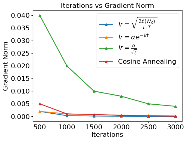
(a)

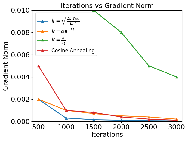
(b)

Figure 1: (a) Plot of iterations v/s $L_{2}$ norm loss function gradient w.r.t trained parameters (b) Magnified version of (a). for more clarity.

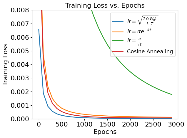
(a)

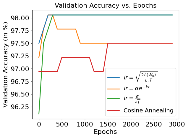
(b)

Figure 2: Plot of (a) Training Loss v/s Epochs (b) Validation Accuracy v/s Epochs

Exp. 3: Effect of initialization. Considering our step size $\alpha\approx\sqrt{\frac{2\mathcal{L}(\textbf{w}_{0})}{KT}}$ is influenced by initial weights $\textbf{w}_{0}$, we varied model initialization using different standard deviations from a standard normal distribution and tracked gradient norms at the start and finish of training, along with the validation accuracy. Table 1 shows that a smaller standard deviation leads to moderate, while larger results in poor. The converged gradient norm trend is convex, while validation accuracy follows a concave pattern. Both worsen with increased initial variance of model weights. Our step size achieves empirical convergence and high validation accuracy when initialized with moderate to low variance.

Table 1: Variation of gradient norm and validation accuracy with respect to initialization (with varying standard deviations)

Std. Dev.	5e-4	1e-3	5e-3	0.01	0.05	0.1	0.5
$\|\nabla\mathcal{L}(\textbf{w}_{0})\|_{2}$	0.02	0.04	0.21	0.38	3.22	15.54	94.49
$\|\nabla\mathcal{L}(\textbf{w}^{*})\|_{2}$	3.6e-5	3e-5	2.6e-5	2.3e-5	2.7e-5	3.3e-5	0.27
Val. Acc. (%)	96.1	96.3	96.4	97.5	97.3	96.4	82.5

5 Conclusion

We provide the first theoretical proof and empirical evidences that deterministic ADAM with a constant step size converges to a critical point for non-convex objectives. Notably, after a specific time threshold $T>T(\sigma)$, the gradient of the loss function trends towards a saddle point. This contrasts with the ADAM variant using a time-dependent step size, which sees its gradient sequence $\{\alpha_{t}\nabla\mathcal{L}(\textbf{w}_{t})\}$ converging to $\boldsymbol{0}$, primarily due to the diminishing $\alpha_{t}$. Our empirical tests further indicate that our step size approach ensures quicker convergence and higher validation accuracy, often targeting a saddle point near a local minimum.

APPENDIX

To Prove. The term $\left((1-\beta_{1})\lambda_{min}(\textbf{A}_{t})-\frac{(\beta_{1}-\beta_{1}^{t})\gamma_{t-1}\lambda_{max}(\textbf{A}_{t})}{\sigma}\right)$ is non-negative.

Proof.

We can construct a lower bound on $\lambda_{min}(\textbf{A}_{t})$ and an upper bound on $\lambda_{min}(\textbf{A}_{t})$ as follows:

$$\lambda_{min}(\textbf{A}_{t})\quad\geq \quad\frac{1}{\epsilon+\sqrt{\underset{1\leq j\leq|\textbf{v}_{t}|}{max}(\textbf{v}_{t})_{j}}}$$ (9)

$$\lambda_{max}(\textbf{A}_{t})\quad\leq \quad\frac{1}{\epsilon+\sqrt{\underset{1\leq j\leq|\textbf{v}_{t}|}{min}(\textbf{v}_{t})_{j}}}$$ (10)

We remember that $\textbf{v}_{t}$ can be rewritten as $\textbf{v}_{t}=\beta_{2}\textbf{v}_{t-1}+(1-\beta_{2})(\nabla\mathcal{L}(\textbf{w}_{t}))^{2}$, solving this recursion and defining $\rho_{t}=\underset{1\leq j\leq t,1\leq k\leq|\textbf{v}_{t}|}{min}(\nabla\mathcal{L}(\textbf{w}_{j})^{2})_{k}$ and taking $\gamma_{t-1}=\gamma_{t}=\gamma$ we have:

$$\lambda_{min}(\textbf{A}_{t})\quad\geq \quad\frac{1}{\epsilon+\sqrt{(1-\beta_{2}^{t})\gamma^{2}}}$$

$$\lambda_{max}(\textbf{A}_{t})\quad\leq \quad\frac{1}{\epsilon+\sqrt{(1-\beta_{2}^{t})\rho_{t}}}$$

Where, $\gamma_{t-1}=\underset{1\leq j\leq t-1}{max}\|\nabla\mathcal{L}(\textbf{w}_{j})\|_{2}$, and $\forall j\in\{1,2,\dots t-1\}$. Setting $\rho_{t}=0$, we can rewrite the term $\left((1-\beta_{1})\lambda_{min}(\textbf{A}_{t})-\frac{(\beta_{1}-\beta_{1}^{t})\gamma_{t-1}\lambda_{max}(\textbf{A}_{t})}{\sigma}\right)$ as:

$$\left((1-\beta_{1})\lambda_{min}(\textbf{A}_{t})-\frac{(\beta_{1}-\beta_{1}^{t})\gamma_{t-1}\lambda_{max}(\textbf{A}_{t})}{\sigma}\right)\geq \hskip 5.0pt\left(\frac{(1-\beta_{1})}{\epsilon+\gamma\sqrt{(1-\beta_{2}^{t})}}-\frac{(\beta_{1}-\beta_{1}^{t})\gamma}{\epsilon\sigma}\right)$$ (11)

$$\geq \hskip 5.0pt\frac{\epsilon\sigma(1-\beta_{1})-\gamma(\beta_{1}-\beta_{1}^{t})(\epsilon+\gamma\sqrt{(1-\beta_{2}^{t})})}{\epsilon\sigma(\epsilon+\gamma\sqrt{(1-\beta_{2}^{t})})}$$

$$\geq \hskip 5.0pt\gamma(\beta_{1}-\beta_{1}^{t})\frac{\epsilon\left(\frac{\sigma(1-\beta_{1})}{\gamma(\beta_{1}-\beta_{1}^{t})}-1\right)-\gamma\sqrt{(1-\beta_{2}^{t})}}{\epsilon\sigma(\epsilon+\gamma\sqrt{(1-\beta_{2}^{t})})}$$

$$\geq \hskip 5.0pt\gamma(\beta_{1}-\beta_{1}^{t})\left(\frac{\sigma(1-\beta_{1})}{\gamma(\beta_{1}-\beta_{1}^{t})}-1\right)\frac{\epsilon-\left(\frac{\gamma\sqrt{(1-\beta_{2}^{t})}}{\frac{(1-\beta_{1}\sigma)}{(\beta_{1}-\beta_{1}^{t})\gamma}-1}\right)}{\epsilon\sigma(\epsilon+\gamma\sqrt{(1-\beta_{2}^{t})})}$$

By definition $\beta_{1}\in(0,1)$ and hence $(\beta_{1}-\beta_{1}^{t})\in(0,\beta_{1})$. This implies that $\frac{(1-\beta_{1})\sigma}{(\beta_{1}-\beta_{1}^{t})\gamma}>\frac{(1-\beta_{1})\sigma}{\beta_{1}\gamma}>1$ where the last inequality follows due to the choice of $\sigma$ as stated in the beginning of this theorem. This allows us to define a constant $\frac{(1-\beta_{1})\sigma}{\beta_{1}\gamma}-1:=\psi_{1}>0$ such that $\frac{(1-\beta_{1})\sigma}{(\beta_{1}-\beta_{1}^{t})\gamma}-1>\psi_{1}$. Similarly, our definition of delta allows us to define another constant $\psi_{2}>0$ to get:

$$\left(\frac{\gamma\sqrt{(1-\beta_{2}^{t})}}{\frac{(1-\beta_{1}\sigma)}{(\beta_{1}-\beta_{1}^{t})\gamma}-1}\right)\quad< \quad\frac{\gamma}{\psi_{1}}=\epsilon-\psi_{2}$$ (12)

Putting Eq.(12) in Eq.(11), we get:

$$\left((1-\beta_{1})\lambda_{min}(\textbf{A}_{t})-\frac{(\beta_{1}-\beta_{1}^{t})\gamma_{t-1}\lambda_{max}(\textbf{A}_{t})}{\sigma}\right)\geq \hskip 5.0pt\left(\frac{\gamma(\beta_{1}-\beta_{1}^{2})\psi_{1}\psi_{2}}{\epsilon\sigma(\epsilon+\sigma)}\right)=c>0$$

∎

References

- [1] Léon Bottou. Stochastic gradient descent tricks. In Neural Networks: Tricks of the Trade. Springer, 2012.
- [2] Léon Bottou. Curiously fast convergence of some stochastic gradient descent algorithms. In Proceedings of the symposium on learning and data science, 2009.
- [3] John Johnson et al. Adaptive subgradient methods for online learning and stochastic optimization. Journal of machine learning research, 2011.
- [4] H Brendan McMahan and Matthew Streeter. Adaptive bound optimization for online convex optimization. arXiv preprint arXiv:1002.4908, 2010.
- [5] Tijmen Tieleman et al. Rmsprop: Divide the gradient by a running average of its recent magnitude. COURSERA Neural Networks Mach. Learn, 17, 2012.
- [6] DP Kingma and J Ba. Adam: A method for stochastic optimization,“u 3rd international conference for learning representations, 2015.
- [7] Matthew D Zeiler. Adadelta: an adaptive learning rate method. arXiv preprint arXiv:1212.5701, 2012.
- [8] Timothy Dozat. Incorporating nesterov momentum into adam, 2016.
- [9] Sharan Vaswani et al. Fast and faster convergence of sgd for over-parameterized models and an accelerated perceptron. In The 22nd international conference on artificial intelligence and statistics, 2019.
- [10] J Reddi Sashank, Kale Satyen, and Kumar Sanjiv. On the convergence of adam and beyond. In International conference on learning representations, 2018.
- [11] James Martens and Roger Grosse. Optimizing neural networks with kronecker-factored approximate curvature. In International conference on machine learning, 2015.
- [12] Soham De, Abhay Yadav, David Jacobs, and Tom Goldstein. Automated inference with adaptive batches. In Artificial Intelligence and Statistics, 2017.
- [13] Babanezhad Harikandeh et al. Stopwasting my gradients: Practical svrg. Advances in Neural Information Processing Systems, 2015.
- [14] Rie Johnson et al. Accelerating stochastic gradient descent using predictive variance reduction. Advances in neural information processing systems, 2013.
- [15] Aaron Defazio et al. Saga: A fast incremental gradient method with support for non-strongly convex composite objectives. Advances in neural information processing systems, 27, 2014.
- [16] Jeremy Bernstein et al. signsgd: Compressed optimisation for non-convex problems. In International Conference on Machine Learning, 2018.
- [17] Naichen Shi, Dawei Li, Mingyi Hong, and Ruoyu Sun. Rmsprop converges with proper hyper-parameter. In International Conference on Learning Representations, 2020.
- [18] Ran Tian and Ankur P Parikh. Amos: An adam-style optimizer with adaptive weight decay towards model-oriented scale. arXiv preprint arXiv:2210.11693, 2022.
- [19] Xiangyi Chen, Sijia Liu, Ruoyu Sun, and Mingyi Hong. On the convergence of a class of adam-type algorithms for non-convex optimization. arXiv preprint arXiv:1808.02941, 2018.
- [20] Liangchen Luo, Yuanhao Xiong, Yan Liu, and Xu Sun. Adaptive gradient methods with dynamic bound of learning rate. arXiv preprint arXiv:1902.09843, 2019.
- [21] Li et al. Jing. Implicit rank-minimizing autoencoder. In Advances in Neural Information Processing Systems, pages 14736–14746, 2020.
- [22] Yunfan Li, Peng Hu, Zitao Liu, Dezhong Peng, Joey Tianyi Zhou, and Xi Peng. Contrastive clustering. In Proceedings of the AAAI conference on artificial intelligence, pages 8547–8555, 2021.
- [23] Soham De, Anirbit Mukherjee, and Enayat Ullah. Convergence guarantees for rmsprop and adam in non-convex optimization and an empirical comparison to nesterov acceleration. arXiv preprint arXiv:1807.06766, 2018.
- [24] Alexandre Défossez, Léon Bottou, Francis Bach, and Nicolas Usunier. A simple convergence proof of adam and adagrad. arXiv preprint arXiv:2003.02395, 2020.
- [25] E. Alpaydin and C. Kaynak. Optical Recognition of Handwritten Digits. UCI Machine Learning Repository, 1998. DOI: https://doi.org/10.24432/C50P49.
- [26] Mahyar Fazlyab et al. Efficient and accurate estimation of lipschitz constants for deep neural networks. Advances in Neural Information Processing Systems, 2019.
- [27] Henry Gouk, Eibe Frank, Bernhard Pfahringer, and Michael J Cree. Regularisation of neural networks by enforcing lipschitz continuity. Machine Learning, 110:393–416, 2021.
- [28] Yusuke Tsuzuku, Issei Sato, and Masashi Sugiyama. Lipschitz-margin training: Scalable certification of perturbation invariance for deep neural networks. Advances in neural information processing systems, 31, 2018.