i-Octree: A Fast, Lightweight, and Dynamic Octree for Proximity Search

Abstract

Establishing the correspondences between newly acquired points and historically accumulated data (i.e., map) through nearest neighbors search is crucial in numerous robotic applications. However, static tree data structures are inadequate to handle large and dynamically growing maps in real-time. To address this issue, we present the i-Octree, a dynamic octree data structure that supports both fast nearest neighbor search and real-time dynamic updates, such as point insertion, deletion, and on-tree down-sampling. The i-Octree is built upon a leaf-based octree and has two key features: a local spatially continuous storing strategy that allows for fast access to points while minimizing memory usage, and local on-tree updates that significantly reduce computation time compared to existing static or dynamic tree structures. The experiments show that i-Octree surpasses state-of-the-art methods by reducing run-time by over 50% on real-world open datasets.

I Introduction

Nearest neighbors search (NNS) is necessary in many robotic applications, such as real-time LiDAR-based simultaneous localization and mapping (SLAM) and motion planning, where the data is sampled sequentially and real-time mapping is essential. For example, in LiDAR-based SLAM, NNS is crucial to compute feature[1, 2], estimate normal[3, 4], and match new points to the map[5, 6, 7, 8]. Recent advances in LiDAR technology have not only significantly reduced the cost, size, weight, and power of LiDAR but also enabled high performance of LiDAR, making it an essential sensor for robots[9]. However, this also poses challenges to NNS. The current LiDAR sensor can produce a large amount of 3D points with centimeter accuracy at hundreds of meters measuring range per second. The large amount of sequential data requires being processed in real-time, which is a quite challenging task on robots with limited onboard computing resources. To guarantee the efficiency of NNS, maintaining a large map supporting high efficient inquiry and dynamic updates with newly arriving points in real-time comes to vital importance.

Although various static tree data structures have been proposed, they struggle to meet the demands. R-tree[10] and R$\ast$-tree[11] partition the data by grouping nearby points into their minimum bounding rectangle in the next higher level of the tree. k-d tree[12] is a well-known instance to split the space. The octree recursively splits the space equally into eight axis-aligned cubes, which form the volumes represented by eight child nodes. Although k-d tree is a favored data structure in general k-nearest neighbors (KNN) search libraries, it is hard to draw any final conclusions as to whether the k-d tree is better suited for NNS compared to other data structures. Comparative studies[13, 14] show that the performance of different implementations of k-d trees can be diverse, and the octree is amongst the best performing algorithms especially for radius search due to its regular partitioning of the search space. Despite its performance, octree has not been fully exploited. Elseberg et al. [15] proposed an efficient octree to store and compress 3D data without loss of precision. Behley et al. [16] proposed an index-based octree that significantly improves the radius neighbor search in three-dimensional data, while the KNN search and dynamic updates are not enabled. When incorporating these static trees in real robotic applications, re-building the entire tree from scratch[17] repeatedly is inevitable, which is so time-consuming that the robots may fail to run.

In this paper, we propose a dynamic octree structure called i-Octree, which incrementally updates the octree with new points and enables fast NNS. In addition, our i-Octree boasts impressive efficiency in both time and memory, adaptable to various types of points, and allows for on-tree down-sampling and box-wise delete. We conduct validation experiments on both randomized data and real-world open datasets to assess the effectiveness of i-Octree. In the randomized data experiments, our i-Octree demonstrates significant improvements in runtime compared to the state-of-the-art incremental k-d tree (i.e., ikd-Tree[9] proposed recently). Specifically, it reduces run-time by 64% for building the tree, 66% for point insertion, 30% for KNN search, and 56% for radius neighbors search. Moreover, when applied to real-world data in LiDAR-based SLAM, i-Octree showcases remarkable time performance enhancements. It achieves over twice the speed of the original method while often maintaining higher accuracy levels. Furthermore, Our implementation of i-Octree is open-sourced on Github.

The remaining paper is organized as follows: the design of i-Octree is described in Section II. Experiments are shown in Section III, followed by conclusions in Section IV.

II i-Octree Design and Implementation

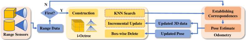
Figure 1: An example of using i-Octree in odometry. The i-Octree and odometry collaborate to estimate the poses of the 3D data obtained from the range sensors. The i-Octree provides a robust and efficient data structure for storing and querying the 3D data, while the odometry enables the estimation of the poses of the data points.

The i-Octree takes sequential point clouds as input with two objectives: dynamically maintains a global map and performs fast NNS (i.e., KNN search and radius neighbors search) on the map. Fig. 1 illustrates a typical application of the i-Octree. The range sensors continuously perceive their surroundings and generate sequential 3D range data periodically. The initial scan of the range data is utilized to construct the i-Octree and define the global coordinate frame. The i-Octree then facilitates the establishment of correspondences between the newly arriving data and the historical data through KNN search or radius neighbors search. Based on these correspondences, the poses of the new data can be estimated, and the 3D points with pose are added to the i-Octree. To prevent the map size in i-Octree from growing uncontrollably, only map points within a large local region (i.e., axis-aligned box) centered around the current position are maintained. In the following, we first describe the data structure and construction of the i-Octree, then we focus on dynamic updates and NNS.

II-A Data Structure and Construction

An i-Octree node has up to eight child nodes, each corresponding to one octant of the overlying axis-aligned cube. An octant, starting with an axis-aligned bounding box with center $\bm{c}\in\mathbb{R}^{3}$ and equal extents $\bm{e}\in\mathbb{R}$, would be subdivided recursively into smaller octants of extent $\frac{1}{2}\bm{e}$ until it contains less than a given number of points – the bucket size $b$ or its extent is less than a minimal extent – $e_{min}$. For memory efficient, octants without points are not created.

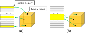
Figure 2: Illustration of locations of a octant’s points in memory. (a) scattered locations; (b) continual locations.

In addition, we only keep indices and coordinates of points in each leaf octant and there is no points in non-leaf octants. To enable extremely fast access to each point in each leaf octant, we propose a local spatially continuous storing strategy (as shown in Fig. 2) which reallocates a segment of continuous memory for storing points information in the leaf octant after subdivision. Furthermore, the reallocation facilitates box-wise delete and incremental update, as it allows operating on a segment of memory without influencing others.

Based on above consideration, an octant $C_{o}$ of our i-Octree contains the center $\bm{c}_{o}\in\mathbb{R}^{3}$, the extent $e_{o}$, the points $\bm{P}_{o}$ storing coordinates and indices, and a pointer pointing to the address of the first child octant. The subscript “o” is used to distinguish between different octants. Particularly, let $C_{r}$ be the root octant, and $\bm{P}_{r},e_{r}$, and $\bm{c}_{r}$ are the points, the extent, and the center, respectively.

As for building an incremental octree, we firstly eliminate invalid points, calculate the axis-aligned bounding box of all valid points, and keep only indices and coordinates of valid points. Then, starting at the root, the i-Octree recursively splits the axis-aligned bounding box at the center into eight cubes indexed by Morton codes[18] and subdivides all the points in current octant into each cube according to their cube indices calculated. When a stopping criteria is satisfied, a leaf octant will be created and a segment of continuous memory will be allocated to store information in points of the leaf node.

II-B Dynamic Updates

The dynamic updates include insertion of one or more points (i.e, incremental update) and delete of all points in an axis-aligned box (i.e., box-wise delete). The insertion is integrated with down-sampling, which maintains the octree at a pre-determined resolution.

II-B1 Incremental Update

When inserting new points, we have to consider the situation that some points may be beyond the boundary of the axis-aligned bounding box of the original tree. Once there are points out of the range of octree, we have to expand the bounding box by creating new root octant whose children contain current root octant.

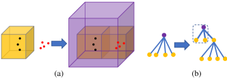
Figure 3: Fig. (a) and (b) illustrate insertion of new points (red) out of the range to the i-Octree. In (a), the left yellow cube is the root octant as well as the leaf octant with points (black) in the beginning. After inserting, the root octant becomes the light purple cube. In (b), the purple node is the root octant and it is updated after inserting new octants (dashed black rectangle).

This process may be executed several times to ensure that all new points are within the range of the tree. Then, new points are added to the expanded octree (see Fig. 3).

In consideration of efficient points queries in robotic applications, i-Octree supports down-sampling that executes simultaneously with point insertion. The down-sampling focuses on the new points and deletes the points that satisfy a certain condition: they are subdivided into a leaf octant whose extent is less than $2e_{min}$ and size is larger than $b/8$.

The process of adding new points to an octant $C_{o}$ is similar to the construction of an octant. If $C_{o}$ is a leaf node and it satisfies the subdivision criteria, all points (i.e., old points and new added points) in $C_{o}$ will be recursively subdivided into child octants. If down-sampling is enabled, $e_{o}\leq 2e_{min}$, and $|\bm{P}_{o}|>b/8$, new points will be deleted later instead of being added to $C_{o}$. Otherwise, a segment of continuous memory will be allocated for the updated points. If $C_{o}$ has child octants, the problem becomes assigning the newly added points to various children, and only the new points are to be subdivided. This process is similar to the one mentioned above, except for the recursive updating of octants.

II-B2 Box-wise Delete

In certain robotic applications, such as SLAM, only the points near the agent are required to estimate the state. Consequently, the points located far away from the agent in the i-Octree are not essential and can be removed for efficiency concerns.

When it comes to removing unnecessary points in an axis-aligned cuboid, instead of directly searching for points within the given space and deleting them, the i-Octree firstly checks whether the octants are inside the given box. All octants inside the given box will be directly deleted without searching for points in them, which significantly reduces the deletion time. The deletion of octants have no influence on others thanks to the local spatially continuous storing strategy.

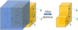
Figure 4: Illustration of box-wise delete. The blue box is the given box, and the numbers 0 to 7 (Morton codes) are the indices of the octants. Octants, with indices 0, 1, 4, and 5 are directly deleted. Octant 7 is also deleted due to having no points.

For the leaf octants overlapping with the given box, we delete the points within the box and allocate a new segment of memory for the remaining. If a leaf octant contains no points after deletion, it will be deleted as shown in Fig. 4.

II-C K-Nearest Neighbors Search

Using i-Octree, we can retrieve $k$ nearest neighbors for an arbitrary query point $\bm{q}\in\mathbb{R}^{3}$. The nearest search on the i-Octree is an accurate nearest search [19] instead of an approximate one as [20]. We maintain a priority queue $\bm{h}$ with a maximal length of $k$ to store the k-nearest neighbors so far encountered and their distance to the query point $\bm{q}$. The last element of $\bm{h}$ always has the largest distance regardless of pushing or popping. The axis-aligned box of each octant is well utilized effectively to accelerate the nearest neighbor search using a “bounds-overlap-ball” test[21] and a proposed priority search order pre-computed according to the fixed indices of child octants.

Firstly, we recursively search down the i-Octree from its root node until reach the leaf node closest to $\bm{q}$. Then the distances from $\bm{q}$ to all points in the leaf node and corresponding indices will be pushed to priority queue $\bm{h}$. All leaf nodes so far encountered will be searched before $\bm{h}$ is full. If $\bm{h}$ is full and the search ball $\bm{S}(\bm{q},d_{max})$ defined by $\bm{q}$ and the largest distance $d_{max}$ in $\bm{h}$ is inside the axis-aligned box of current octant, the searching is over. If a octant $C_{k}$ doesn’t contain the search ball $\bm{S}(\bm{q},d_{max})$, then one of the following three conditions must be satisfied:

$$e_{k}-|{q}_{x}-{c}_{k,x}|<d_{max},$$ (1)

$$e_{k}-|{q}_{y}-{c}_{k,y}|<d_{max},$$ (2)

$$e_{k}-|{q}_{z}-{c}_{k,z}|<d_{max},$$ (3)

where $\bm{q}=({q}_{x},{q}_{y},{q}_{z})^{T},\bm{c}_{k}=({c}_{k,x},{c}_{k,y},{c}_{k,z})^{T}$. If none of the above conditions hold, the search ball is inside the octant.

We update $\bm{h}$ by investigating octants overlapping the search ball $\bm{S}(\bm{q},d_{max})$, since only these could potentially contain points that are also inside the desired neighborhood. We define the distance $d$ between $\bm{q}$ and $C_{k}$ as below:

$$d=\rVert\sigma(|\bm{q}-\bm{c}_{o}|-\bm{1}e_{o})\lVert_{2},$$ (4)

where $\bm{1}=(1,1,1)^{T}$ and $\sigma(x)=x$ if $x>0$, otherwise $\sigma(x)=0$. $d<d_{max}$ indicates that $C_{k}$ overlaps $\bm{S}(\bm{q},d_{max})$. In order to speed up the process, we sort the candidate child octants of $C_{o}$ according to their distances to $C_{k}$ and get 8 different sequences in $\bm{I}_{order}$. Such that the closer octants are earlier to be searched and the search reaches its end early.

II-D Radius Neighbors Search

For an arbitrary query point $\bm{q}\in\mathbb{R}^{3}$ and radius $r$, the radius neighbors search method finds every point $\bm{p}$ satisfying $\lVert\bm{p}-\bm{q}\rVert_{2}<r$. The process is similar to KNN search except for a fixed radius and an unlimited $k$. We adopt the pruning strategy proposed by Behley et al. [16] with improvements to reduce computation cost. Before test whether $\bm{S}(\bm{q},r)$ completely contains an octant $C_{k}$, we make a simple test whether $r^{2}$ is larger than $3e_{k}^{2}$. The simple test is the necessary condition for $\bm{S}(\bm{q},r)$ containing $C_{k}$ with small cost. Besides, we try to avoid the extraction of a root in the algorithm. These two tricks together with our local spatially continuous storing strategy play key roles in accelerating the searching.

III Application Experiments

We compare our i-Octree to publicly available implementations of static k-d trees (i.e., k-d tree used in Point Cloud Library (PCL)) , incremental k-d tree (i.e., ikd-Tree), and PCL octree. We conduct the experiments on randomized data and various open real-world datasets. We first evaluate our i-Octree against PCL octree and the state-of-the-art incremental k-d tree, i.e., ikd-Tree, for tree construction, point insertion, KNN search, radius neighbors search, and box-wise delete on randomized three dimensional (3D) point data of different size. Then, we validate the i-Octree in actual robotic applications on real-world dataset by replacing the static k-d tree in the LiDAR-based SLAM without any refinement and evaluate the time performance and accuracy. All experiments are performed on a PC with Intel i7-13700K CPU at 3.40GHz.

III-A Randomized Data Experiments

The efficiency of our i-Octree is fully investigated by the following experiments on randomized incremental data.

III-A1 Performance Comparison

In this experiment, we investigate the time performance of three implementations of dynamic data structure (i.e., the i-Octree, the ikd-Tree, and the PCL octree). Both ikd-Tree and PCL octree are state-of-the-art implementations with high efficiency and support point insertion, which is the key consideration why we choose them to be compared with our i-Octree for a fair comparison. In this experiment, we adopt the same setup as above with fixed $b$ and $e_{min}$. Besides, down-sampling is not enabled on i-Octree and ikd-Tree. We record the time for tree construction and point insertion, the total time of kNN search for 200 points, and the total time of radius neighbors search for another 200 points at each step.

The dynamic data structure comparison over different tree size is shown in Fig. 5 and the Table I shows the comparison of average time consumption.

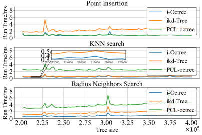
Figure 5: Dynamic data structure comparison over different tree size.

When the tree size increases from 200,000 to 400,000, the time for point insertion (without down-sampling) of i-Octree and PCL octree remains stable at 0.8$ms$ while that for the ikd-Tree is 3 times larger and grows linearly with the tree size.

TABLE I: The Comparison of Average Time Consumption

	i-Octree[ms]	ikd-Tree[ms]	PCL-octree[ms]
Construction1	16.63	46.26	52.66
Point Insertion	0.83	2.45	0.85
KNN Search	0.41	0.59	2.53
Radius Neighbors Search	0.81	1.85	3.96

• The construction of the tree is conducted only once at the first time.

Even the peak insertion time of i-Octree is less than the regular insertion time of ikd-Tree. The time for KNN search of the three implementations is stable. Our method runs 6 times faster than the PCL octree and reduces the run time by 33% over the ikd-Tree. As for the time taken for radius neighbors search, the i-Octree exhibits the slowest growth, running approximately 2 times faster than the ikd-Tree and 5 times faster than the PCL octree. Besides, the construction time of the i-Octree is only 36% of that of ikd-Tree and 31% of that of PCL octree.

III-A2 Box-wise Delete

The ikd-Tree is chosen to be compared with the i-Octree since both support the box-wise delete. This experiment investigates the time performance of deleting all points in an axis-aligned box and the time performance of KNN serach and radius neighbors search after delete. In the experiment, we sample 400,000 points randomly in a $10m\times 10m\times 10m$ space (i.e., the workspace) to initialize the incremental octree. Then 1,00 test operations are conducted on the trees.

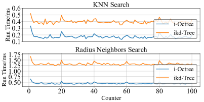
Figure 6: The comparison of time consumption.

In each test operation, we randomly sample 200 points in the workspace for KNN search and another 200 points for radius neighbors search. For every 20 test operations, one axis-aligned box is sampled in the workspace with side length of $1.0m$ and points contained in the box are deleted from the trees. We record the tree size after each delete, the time of box-wise delete, the total time of kNN search for 200 points, and the total time of radius neighbors search for another 200 points at each step.

The time of box-wise delete and the tree size are shown in Table II.

TABLE II: The Time Consumption of Box-wise Delete and Tree Size

Counter	Box-wise Delete[ms]		Tree Size
	i-Octree	ikd-Tree	GT1	i-Octree	ikd-Tree
0	–	–	400,000	400,000	400,000
20	0.017	0.222	399,614	399,614	399,623
40	0.013	0.343	399,205	399,205	399,236
60	0.017	0.250	398,783	398,783	398,826
80	0.016	0.320	398,375	398,375	398,437
100	0.006	0.126	398,185	398,185	398,247

• GT denotes the exact size of the point cloud at each test.

The run time performance of i-Octree and ikd-Tree on KNN search and radius neighbors search is shown in Fig. 6. In this experiment, it appears that the box-wise delete operation on the ikd-Tree does not remove all points within the given box as shown in Table II. The results show that our i-Octree runs over 10 times faster than the ikd-Tree on the box-wise delete and approximately 3 times faster on the radius neighbors search. Besides, the i-Octree reduces the run time of KNN search by 58% over the ikd-Tree.

III-B Real-world Data Experiments

We test our developed i-Octree in actual robotic applications (e.g., LiDAR-inertial SLAM[22, 8, 23] and pure LiDAR SLAM[24, 6, 5]). In these experiments, we directly replace the static k-d tree in the LiDAR-based SLAM by our proposed i-Octree without any refinement and evaluate the time performance and accuracy. To ensure a fair and complete comparison, we test on three datasets: M2DGR[25], Newer College Dataset[26] and NCLT[27] with different sensor setups. The M2DGR is a low-beam LiDAR data, the Newer College Dataset is a high-beam LiDAR data, and the NCLT is a long-term dataset. They all have ground truth trajectories such that we can evaluate the accuracy of the LiDAR trajectories using absolute trajectory error (ATE)[28].

For the sake of simplicity, we will focus on two representative LiDAR-based SLAM algorithms: LIO-SAM[22] that combines LiDAR and inertial measurements (LiDAR-inertial SLAM), and FLOAM[24] that relies solely on LiDAR data (pure LiDAR SLAM). Both are the state-of-the-art algorithms and uses the static k-d tree for the nearest points search, which is crucial to match a point in a new LiDAR scan to its correspondences in the map (or the previous scan). For the LIO-SAM, we choose the LIO_SAM_6AXIS, which is modified from LIO-SAM to support a wider range of sensors (e.g., 6-axis IMU and low-cost GNSS) without accuracy loss. Besides, the loop closure module of LIO_SAM_6AXIS is deactivated. The parameters setups, as shown in Table III, for every sequence in a dataset are the same.

TABLE III: The Parameters Setup for each dataset

Dataset	FLOAM			LIO_SAM_6AXIS
	SurfRes	EdgeRes	MinRange	SurfRes	EdgeRes	MinRange
M2DGR	0.1m	0.05m	0.2m	0.4m	0.2m	1.0m
Newer College	0.2m	0.1m	0.2m	0.4m	0.2m	1.0m
NCLT	0.4m	0.2m	0.2m	0.4m	0.2m	1.0m

• SurfRes and EdgeRes denote the map resolution of surface map and edge map, respectively; MinRange means that any points within the LiDAR range defined by MinRange will not be considered.

Both algorithms build two independent maps: surface map and edge map, where two k-d trees or i-Octree will be built. The SurfRes and EdgeRes determine the minimal extent of the two i-Octree structures, respectively.

III-B1 Low-beam LiDAR Data

The first dataset is M2DGR, which is a large-scale dataset collected by an unmanned ground vehicle (UGV) with a full sensor-suite including a Velodyne VLP-32C LiDAR sampled at 10 $Hz$, a 9-axis Handsfree A9 inertial measurement unit (IMU) sampled at 150 $Hz$, and other sensors.

TABLE IV: The Selected Sequences From M2DGR

Sequence Name	Duration	Type	Features
gate_01	172s	Outdoor	dark,around gate
gate_02	327s	Outdoor	dark,loop back
walk_01	291s	Outdoor	day,back and fourth
street_02	1227s	Outdoor	day,long-term
street_03	354s	Outdoor	night,full speed
room_01	72s	Indoor	room,bright
room_02	75s	Indoor	room,bright
room_dark_01	111s	Indoor	room,dark

The dataset comprises 36 sequences captured in diverse scenarios including both indoor and outdoor environments on the university campus. The ground truth trajectories of the outdoor sequences are obtained by the Xsens MTi 680G GNSS-RTK suite while for the indoor environment, a motion-capture system named Vicon Vero 2.2 whose localization accuracy is 1$mm$ is used to collect the ground truth. We choose several sequences from this dataset and the detailed information is summarized in Table IV.

The maximal and average time consumption of incremental update, as well as the maximal and average total time consumption for each scan, are listed in Table V.

TABLE V: The Comparison of Time Consumption per Scan on Incremental Update and Total Time

Sequence Name	FLOAM[ms]								LIO_SAM_6AXIS[ms]
	Incre_max		Incre_mean		Total_max		Total_mean		Incre_max		Incre_mean		Total_max		Total_mean
	ioct	orig	ioct	orig	ioct	orig	ioct	orig	ioct	orig	ioct	orig	ioct	orig	ioct	orig
gate_01	7.20	969.98	5.57	354.73	210.42	1403.39	101.70	570.62	5.16	33.99	2.82	17.56	802.45	1256.75	40.69	100.50
gate_02	7.79	1227.55	5.19	514.61	231.84	1733.16	90.37	787.82	5.49	28.50	2.69	15.89	147.87	167.01	25.32	71.29
walk_01	6.92	271.49	5.17	141.08	202.57	468.67	91.21	273.72	4.66	15.39	2.53	11.18	79.39	85.46	18.98	52.42
street_02	7.07	793.63	4.20	286.17	222.03	1148.53	82.85	462.21	6.95	19.88	2.94	10.84	152.52	143.86	24.26	58.05
street_03	9.22	1983.50	6.52	893.20	221.25	2784.90	117.55	1318.47	7.27	30.05	3.58	19.57	127.28	265.98	39.11	114.55
room_01	2.22	17.41	0.64	5.67	67.67	81.11	22.42	25.91	0.42	1.70	0.29	0.48	72.96	137.20	3.11	12.32
room_02	3.00	24.00	0.65	6.30	70.83	85.08	22.52	26.60	0.43	0.73	0.28	0.46	79.85	83.01	3.02	6.32
room_dark_01	2.48	13.57	0.71	6.13	80.39	82.95	22.85	26.16	0.52	0.74	0.29	0.44	65.57	90.10	2.70	5.73

• Note: Incre_max and Incre_mean denote the maximal and average incremental update time of each scan respectively; Total_max and Total_mean denote the maximal and average total time consumption for each scan; ioct means i-Octree and orig means the static k-d tree.

For the LOAM running in the outdoor environment, the size of map grows gradually making it computational costly when using the static k-d tree. The rebuilding process may cost a lot when the size of map is large, which deteriorates the real-time performance sharply. The time for rebuilding the entire k-d tree fills a large percentage of the total time per scan, as shown in the Fig. 7.

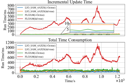
Figure 7: The Comparison of time consumption on the street_02 sequence.

After replacing the k-d tree by i-Octree, the incremental time reduces to less than 10$ms$ and the real-time performance is approximately guaranteed. The FLOAM with i-Octree runs over 5 times faster than the original one, with sometimes a slight accuracy loss as shown in Table VI.

TABLE VI: Absolute Translational Errors (RMSE, meters) in Sequences With Good Quality Ground Truth

Sequence Name	FLOAM		LIO_SAM_6AXIS
	i-Octree	static k-d tree	i-Octree	static k-d tree
gate_01	8.667	9.206	0.167	0.340
gate_02	13.638	9.620	0.325	0.314
walk_01	0.108	0.087	0.078	0.079
street_02	133.602	80.935	2.296	2.942
street_03	15.781	16.923	0.137	0.138
room_01	0.134	0.135	0.137	0.209
room_02	0.128	0.129	0.123	0.121
room_dark_01	0.146	0.148	0.151	0.155

The LIO_SAM_6AXIS with i-Octree runs over 2 times faster than original one on almost all sequences and the accuracy is usually improved. Besides, the i-Octree reduces the peak time which degrades the real-time ability.

III-B2 High-beam LiDAR Data

The second dataset is the Newer College Dataset, which is a multi-camera LiDAR inertial dataset of 4.5 $km$ walking distance. The dataset is collected by a handheld device equipped with an Ouster OS0-128 LiDAR sampled at 10 $Hz$ with embedded IMU sampled at 100 $Hz$. Precise centimetre accurate ground truth is provided and calculated by registering each undistorted LiDAR frame to a prior map scanned by 3D imaging laser scanner, Leica BLK360.

TABLE VII: The Selected Sequences From Newer College Dataset

Sequence Name	Duration	Length	Features
Quad-Easy	198s	247m	loops, walking speed
Quad-Medium	190s	260m	loops, brisk walking
Quad-Hard	187s	234m	fast, aggressive motion
Cloister	278s	429m	loops, cloister corridor
Maths-Easy	216s	264m	large scale
Underground-Easy	141s	162m	underground mine

Table VII shows the 6 sequences selected from the dataset. These sequences contain small and narrow passages, large scale open spaces, as well as vegetated areas. Besides, challenging situations such as aggressive motion are presented.

In this test, we only record average total time consumption of each scan, as shown in Table VIII, and calculate the RMSE of the absolute translational errors, as shown in Table IX.

TABLE VIII: The Comparison of Total Time Consumption per Scan

Sequence Name	FLOAM[[ms]		LIO_SAM_6AXIS[ms]
	i-Octree	static k-d tree	i-Octree	static k-d tree
Quad-Easy	73.87	225.31	38.03	100.73
Quad-Medium	58.19	430.78	43.02	96.86
Quad-Hard	44.86	300.38	32.85	70.35
Cloister	41.06	156.80	20.07	53.77
Maths-Easy	62.53	180.89	31.34	74.46
Underground-Easy	28.16	41.27	9.37	30.85
2012-01-08	21.88	70.62	24.65	53.54

We find that the i-Octree shows promising compatibility with LIO_SAM_6AXIS since it not only reduces the time consumption a lot but also improves the accuracy. For the LOAM, the i-Octree significantly accelerates the processing speed per scan, but sometimes at a cost of degrading accuracy, as it directly replaces the static k-d tree without any refinement.

III-B3 Long-term LiDAR Data

Finally, we test on a long sequence called 2012-01-08 form a large scale dataset named NCLT captured by a Velodyne HDL-32E LiDAR sampled at 10 $Hz$, a Microstrain 3DM-GX3-45 IMU sampled at 100 $Hz$, and other sensors. The length of the sequence is 6.4$km$ and the duration is 5633s. The average run time of each scan is added in Table VIII, and the absolute translational errors are added to Table IX.

TABLE IX: Absolute Translational Errors (RMSE, meters) in Sequences With Ground Truth

Sequence Name	FLOAM		LIO_SAM_6AXIS
	i-Octree	static k-d tree	i-Octree	static k-d tree
Quad-Easy	0.795	0.399	0.083	0.079
Quad-Medium	15.626	18.358	0.100	0.095
Quad-Hard	17.133	7.326	0.130	0.152
Cloister	15.100	7.685	0.115	0.169
Maths-Easy	1.026	0.260	0.088	0.125
Underground-Easy	0.143	0.078	0.077	0.073
2012-01-08	187.588	62.188	1.890	9.291

The FLOAM drifts severely on the large scale sequence while LIO_SAM_6AXIS (i-Octree) shows surprising performance, except for a slight drift along the z-axis, even without enabling loop closure. LIO_SAM_6AXIS (static k-d tree) can only use the very recent key frames to estimate the poses, whereas LIO_SAM_6AXIS (i-Octree) can take advantage of point information from the start, which contributes to its better performance.

IV Conclusion

In this paper, we propose a novel dynamic octree data structure, i-Octree, which supports incrementally point insertion with on-tree down-sampling, box-wise delete, and fast NNS. Besides, a large amount of experiments on both randomized datasets and open datasets show that our i-Octree can achieve the best overall performance among the state-of-the-art tree data structures.

References

- [1] X. Xiong, D. Munoz, J. A. Bagnell, and M. Hebert, “3-d scene analysis via sequenced predictions over points and regions,” in 2011 IEEE International Conference on Robotics and Automation, 2011, pp. 2609–2616.
- [2] J. Behley, V. Steinhage, and A. B. Cremers, “Performance of histogram descriptors for the classification of 3d laser range data in urban environments,” in 2012 IEEE International Conference on Robotics and Automation, 2012, pp. 4391–4398.
- [3] N. J. Mitra and A. Nguyen, “Estimating surface normals in noisy point cloud data,” in Proceedings of the Nineteenth Annual Symposium on Computational Geometry, ser. SCG ’03. New York, NY, USA: Association for Computing Machinery, 2003, p. 322–328. [Online]. Available: https://doi.org/10.1145/777792.777840
- [4] K. Klasing, D. Wollherr, and M. Buss, “A clustering method for efficient segmentation of 3d laser data,” in 2008 IEEE International Conference on Robotics and Automation, 2008, pp. 4043–4048.
- [5] J. Zhang and S. Singh, “Loam: Lidar odometry and mapping in real-time.” in Robotics: Science and Systems, vol. 2, no. 9, 2014.
- [6] T. Shan and B. Englot, “Lego-loam: Lightweight and ground-optimized lidar odometry and mapping on variable terrain,” in 2018 IEEE/RSJ International Conference on Intelligent Robots and Systems (IROS). IEEE, 2018, pp. 4758–4765.
- [7] J. Lin and F. Zhang, “Loam livox: A fast, robust, high-precision lidar odometry and mapping package for lidars of small fov,” in 2020 IEEE International Conference on Robotics and Automation (ICRA). IEEE, 2020, pp. 3126–3131.
- [8] W. Xu and F. Zhang, “Fast-lio: A fast, robust lidar-inertial odometry package by tightly-coupled iterated kalman filter,” arXiv preprint arXiv:2010.08196, 2020.
- [9] W. Xu, Y. Cai, D. He, J. Lin, and F. Zhang, “Fast-lio2: Fast direct lidar-inertial odometry,” IEEE Transactions on Robotics, vol. 38, no. 4, pp. 2053–2073, 2022.
- [10] A. Guttman, “R-trees: A dynamic index structure for spatial searching,” in Proceedings of the 1984 ACM SIGMOD international conference on Management of data, 1984, pp. 47–57.
- [11] N. Beckmann, H.-P. Kriegel, R. Schneider, and B. Seeger, “The r*-tree: An efficient and robust access method for points and rectangles,” in Proceedings of the 1990 ACM SIGMOD international conference on Management of data, 1990, pp. 322–331.
- [12] J. L. Bentley, “Multidimensional binary search trees used for associative searching,” Communications of the ACM, vol. 18, no. 9, pp. 509–517, 1975.
- [13] J. L. Vermeulen, A. Hillebrand, and R. Geraerts, “A comparative study of k-nearest neighbour techniques in crowd simulation,” Computer Animation and Virtual Worlds, vol. 28, no. 3-4, p. e1775, 2017.
- [14] J. Elseberg, S. Magnenat, R. Siegwart, and A. Nüchter, “Comparison of nearest-neighbor-search strategies and implementations for efficient shape registration,” Journal of Software Engineering for Robotics, vol. 3, no. 1, pp. 2–12, 2012.
- [15] J. Elseberg, D. Borrmann, and A. Nüchter, “One billion points in the cloud–an octree for efficient processing of 3d laser scans,” ISPRS Journal of Photogrammetry and Remote Sensing, vol. 76, pp. 76–88, 2013.
- [16] J. Behley, V. Steinhage, and A. B. Cremers, “Efficient radius neighbor search in three-dimensional point clouds,” in 2015 IEEE International Conference on Robotics and Automation (ICRA), 2015, pp. 3625–3630.
- [17] R. B. Rusu and S. Cousins, “3d is here: Point cloud library (pcl),” in 2011 IEEE international conference on robotics and automation. IEEE, 2011, pp. 1–4.
- [18] G. M. Morton, “A computer oriented geodetic data base and a new technique in file sequencing,” International Business Machines Company, New York, Tech. Rep., 1996.
- [19] J. H. Friedman, J. L. Bentley, and R. A. Finkel, An algorithm for finding best matches in logarithmic time. Department of Computer Science, Stanford University, 1975.
- [20] M. Muja and D. G. Lowe, “Fast approximate nearest neighbors with automatic algorithm configuration.” VISAPP (1), vol. 2, no. 331-340, p. 2, 2009.
- [21] J. H. Friedman, J. L. Bentley, and R. A. Finkel, “An algorithm for finding best matches in logarithmic expected time,” ACM Trans. Math. Softw., vol. 3, no. 3, p. 209–226, sep 1977. [Online]. Available: https://doi.org/10.1145/355744.355745
- [22] T. Shan, B. Englot, D. Meyers, W. Wang, C. Ratti, and D. Rus, “Lio-sam: Tightly-coupled lidar inertial odometry via smoothing and mapping,” in 2020 IEEE/RSJ international conference on intelligent robots and systems (IROS). IEEE, 2020, pp. 5135–5142.
- [23] K. Li, M. Li, and U. D. Hanebeck, “Towards high-performance solid-state-lidar-inertial odometry and mapping,” IEEE Robotics and Automation Letters, vol. 6, no. 3, pp. 5167–5174, 2021.
- [24] H. Wang, C. Wang, C.-L. Chen, and L. Xie, “F-loam: Fast lidar odometry and mapping,” in 2021 IEEE/RSJ International Conference on Intelligent Robots and Systems (IROS). IEEE, 2021, pp. 4390–4396.
- [25] J. Yin, A. Li, T. Li, W. Yu, and D. Zou, “M2dgr: A multi-sensor and multi-scenario slam dataset for ground robots,” IEEE Robotics and Automation Letters, vol. 7, no. 2, pp. 2266–2273, 2021.
- [26] L. Zhang, M. Camurri, D. Wisth, and M. Fallon, “Multi-camera lidar inertial extension to the newer college dataset,” 2021.
- [27] N. Carlevaris-Bianco, A. K. Ushani, and R. M. Eustice, “University of Michigan North Campus long-term vision and lidar dataset,” International Journal of Robotics Research, vol. 35, no. 9, pp. 1023–1035, 2015.
- [28] J. Sturm, N. Engelhard, F. Endres, W. Burgard, and D. Cremers, “A benchmark for the evaluation of rgb-d slam systems,” in 2012 IEEE/RSJ international conference on intelligent robots and systems. IEEE, 2012, pp. 573–580.