Large Intestine 3D Shape Refinement Using Point Diffusion Models for Digital Phantom Generation

Abstract

Accurate 3D modeling of human organs plays a crucial role in building computational phantoms for virtual imaging trials. However, generating anatomically plausible reconstructions of organ surfaces from computed tomography scans remains challenging for many structures in the human body. This challenge is particularly evident when dealing with the large intestine. In this study, we leverage recent advancements in geometric deep learning and denoising diffusion probabilistic models to refine the segmentation results of the large intestine. We begin by representing the organ as point clouds sampled from the surface of the 3D segmentation mask. Subsequently, we employ a hierarchical variational autoencoder to obtain global and local latent representations of the organ’s shape. We train two conditional denoising diffusion models in the hierarchical latent space to perform shape refinement. To further enhance our method, we incorporate a state-of-the-art surface reconstruction model, allowing us to generate smooth meshes from the obtained complete point clouds. Experimental results demonstrate the effectiveness of our approach in capturing both the global distribution of the organ’s shape and its fine details. Our complete refinement pipeline demonstrates remarkable enhancements in surface representation compared to the initial segmentation, reducing the Chamfer distance by 70%, the Hausdorff distance by 32%, and the Earth Mover’s distance by 6%. By combining geometric deep learning, denoising diffusion models, and advanced surface reconstruction techniques, our proposed method offers a promising solution for accurately modeling the large intestine’s surface and can easily be extended to other anatomical structures.

Digital Phantom, Denoising Diffusion Models, Geometric Deep Learning, Large Intestine Modeling, 3D Shape Refinement.

1 Introduction

In virtual imaging trials, realistic digital phantoms are crucial as they serve as virtual patients for simulated studies. Together with imaging and diagnostic simulation tools, they allow researchers to conduct iterative experiments with limitless parameter combinations, reducing concerns about potential side effects like excessive radiation exposure.[1, 2, 3]. A typical pipeline of creating computerized patient models involves collecting imaging data from real patients, segmenting the chosen organs, and then converting the resulting masks into easily deformable mathematical representations like polygon meshes.[4]. The segmentation step is crucial in the process, as its outcomes greatly influence the quality of the generated phantoms. Early studies mainly relied on either manual contouring[4] or conventional image processing-based segmentation algorithms, such as thresholding[5], for this purpose. The fast development of deep learning (DL) segmentation algorithms, along with greater access to radiological images, has led to a variety of DL-based medical image segmentation approaches. These methods have proven their accuracy in segmenting multiple organs from computed tomography (CT) scans.[6, 7]. Notably, TotalSegmentator[8], a prominent DL model, has achieved state-of-the-art segmentation performance in this domain. Even though these methods significantly outperform their traditional counterparts, the challenge of medical image segmentation is still far from being solved[9].

This task is particularly challenging for the large intestine where the segmented surfaces often exhibit disconnected surfaces, and incorporate sections of adjacent organs such as the small intestine, or organs that exhibit similar features such as the presence of air in the stomach. These issues stem from two main factors. Firstly, the large intestine’s complexity which arises from low soft tissue contrast, heterogeneous filling, varying shapes and sizes among patients, proximity to low-contrast abdominal organs, and the impact of filling status on its shape.[10]. Secondly, current DL algorithms, such as U-Nets[11], rely on volumetric Convolutional Neural Networks (CNNs) which accurately recover organ volumes. However, they struggle in obtaining precise surface representations due to several factors: these models do not account for shape constraints and produce discrete voxel grids, leading to discretization effects when converted to surface representations, ultimately resulting in anatomically inaccurate shapes.[12, 13]. Under these conditions, the shapes of the large intestine require manual inspection and refinement by an expert before being incorporated into the digital phantom. This process is laborious, time-consuming, and subjective, highlighting the necessity for an automated approach to achieve anatomically accurate 3D representations of the organ starting from an imperfect segmentation result.

3D shape completion and refinement is extensively studied in various domains, including autonomous driving, robotics, and manufacturing[14, 15]. In these fields, LiDAR sensors are frequently employed to detect objects, leading to sparse, noisy, and partial shapes represented as point clouds. Therefore, the development of tools for shape completion, denoising, and refinement becomes essential. In recent years, a notable advancement has emerged in the processing of complex 3D data, particularly with the introduction of geometric deep networks such as PointNets [16]. Unlike traditional CNNs that operate on volumetric data, PointNets are explicitly designed for processing point cloud data, enabling more efficient and effective analysis of 3D shapes and surfaces. The use of such geometric models has been explored in medical imaging for different tasks[17, 12]. Balsiger et al.[18] present a point cloud-based approach to refine peripheral nervous system segmentations. This method utilizes a CNN to segment the nervous system and extract image information from an MRN volume. Point clouds are then extracted from the mask’s surface, and their xyz-coordinates are combined with the deep image features. Using a PointCNN[19], each point is classified as foreground or background to refine the segmentation and eliminate noise. However, although this approach effectively addresses false positives, it does not recover false negatives overlooked by the segmentation network. Recently, denoising diffusion probabilistic models (DDPMs) [20] have demonstrated remarkable outcomes in completing missing data whether it pertains to 1D signals like speech, 2D representations like images, or 3D structures such as object shapes[21, 22, 23]. Example applications of diffusion models in the field of 3D shape processing include the latent Point Diffusion Model (LION) for shape generation[24]. LION employs a variational autoencoder (VAE) with a hierarchical latent space, combining global and local representations. By training DDPMs in this smoother latent space, the model can better capture shape distributions and generate higher-quality shapes. LION has achieved state-of-the-art performance on benchmarks and can be extended to other applications like text-to-shape generation. For shape completion, Lyu et al. [25] propose a Point Diffusion-Refinement (PDR) approach comprising a Conditional Generation Network (CGNet) and a Refinement Network (RFNet). CGNet is a conditional DDPM, generating a coarse complete point cloud from partial input, while RFNet densifies the point cloud for quality improvement. Both networks utilize a dual-path architecture based on PointNet++[26] for efficient feature extraction from partial shapes and precise manipulation of 3D point locations. Friedrich et al. [27] propose an Application of point diffusion models on a medical imaging task. The method uses Zhou et al.’s point-voxel diffusion (PVD) method [23] for 3D skull implant generation. The model is trained to create a complete skull shape from a defective one. Only points belonging to the implant are modified during the diffusion process, while those in the defective structure remain unchanged. This approach effectively generates missing false negative points, but it cannot remove false positive points because they remain fixed throughout the diffusion process.

In this research, we aim to address the issue of inaccurate surface reconstructions of the large intestine resulting from a volumetric segmentation model by leveraging the latest advancements in geometric deep learning and DDPMs. Our approach diverges from the one proposed by Balsiger et al.[18], as we incorporate generative geometric models capable of generating new points to fill in the missing parts of the organ’s shape representation. To tackle the problem of false positives, we propose using a method based on extracting features from the erroneous shapes to guide the refinement process, without fixing them during the diffusion process, which contrasts with the approach suggested by Friedrich et al.[27]. Specifically, we represent the shapes as point clouds and employ latent denoising diffusion models with PointNet-based backbones, conditioned on the partial shapes of the organ, to generate complete shapes as outputs. Additionally, we employ a modern surface reconstruction method to represent the final outputs as polygon meshes, which is a preferred representation in computational phantoms. The contributions of this work can be summarized as follows:

• To the best of our knowledge, we are the first to tackle the problem of large intestine shape refinement as a conditional point cloud generation task.

• We construct a dataset consisting of pairs of 3D large intestine shapes. Each pair includes an erroneous shape generated by a deep learning model and the corresponding ground truth.

• Drawing inspiration from LION[24] and PDR[25] , we introduce a novel method for point cloud refinement. Our approach involves training conditional point-diffusion models within a hierarchical latent space.

• We propose a simple point cloud post-processing pipeline that effectively increases the density and smooths out the noisy clouds before performing surface reconstruction.

2 Material and Methods

This section provides a comprehensive overview of our research methodology. Firstly, we describe the dataset generation procedure. Subsequently, we present the baseline approach that serves as a reference for our study. Next, we introduce our novel method, specifically designed to enhance and optimize the results. Finally, we detail the post-processing and surface reconstruction pipeline.

2.1 Dataset

We created a dataset that includes pairs of erroneous and correct 3D shapes of the large intestine. Our data include one public and two private datasets.

2.1.1 TotalSegmentator Dataset

Wasserthal et al. [8] provide a public dataset of 1024 CT scans with reference masks for the large intestine (referred to as ”colon”). The dataset contains various CT types, some of which lack the large intestine entirely (e.g., head CTs) or only contain parts of it. we established a set of rules to extract cases with complete large intestines based on connected component analysis and the organ volume distributions derived from the provided reference masks:

• Cases with a stomach volume lower than 50ml and a urinary bladder volume of 0ml are eliminated, thus ensuring the upper and lower bounds of the intestine are present.

• Outlier cases with large intestine volume lower than 400ml or higher than 1500ml are eliminated.

• Binary closing operations were performed to close small disconnections in the remaining cases that have more than two components (Background+large intestine).

• From the remaining cases, only those with two connected components are kept.

The number of remaining cases after the selection process is 308.

2.1.2 Duke PET/CT Dataset

This set comprises 112 CT volumes from Duke Hospital patients’ Positron Emission Tomography and Computed Tomography (PET/CT) scans. We used TotalSegmentator’s pre-trained model to obtain segmentation masks for the large intestine. Further analysis for extracting the successful cases involved removing components smaller than 500 voxels and applying binary closing to address minor disconnections. The remaining cases with more than two components were excluded, resulting in 75 remaining cases.

2.1.3 Duke CAP Dataset

The set includes 269 Chest Abdomen Pelvis (CAP) CT scans from Duke Hospital patients. The samples underwent the same pipeline as the PET/CT cases. Additionally, a physician refined 34 cases with incorrect masks resulting in a total of 195 cases.

2.1.4 Partial Shape Synthesis

To train a model that refines erroneous organ shapes within a supervised learning framework, we needed a dataset of example failure cases that will be used as model inputs together with the corresponding correct shapes which will be used as the target outputs. Having the previously selected correct shapes, we needed to generate synthetic erroneous masks that mimic the behavior of TotalSegmentator’s failures illustrated in fig. 1. For this purpose, we built a weak 3D full-resolution U-Net model by training nn-Unet[28] for 30 epochs using 30 images randomly selected from our TotalSegmentator subset. We run inference using this model on all cases in our dataset to obtain the defective segmentation masks.

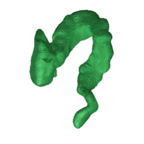
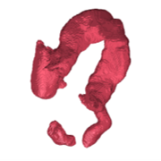
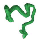
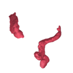
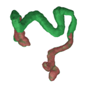
[5pt]   [5pt]   [5pt]
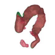
[5pt]Reference   [5pt]Model output   [5pt]Overlap

Figure 1: Examples of erroneous TotalSegmentator results with the corresponding references annotated by a physician. The segmentation failures include false positives included from other organs (upper row) and missing components (lower row).

2.1.5 Point Cloud Extraction

After obtaining the pairs of erroneous and reference masks, we run the marching cubes algorithm[29] to extract the organ surfaces represented as polygon meshes. Later, we used the Poisson disk sampling algorithm[30] to sample point clouds of 2048 points from the surfaces of the meshes. This algorithm extracts points such that each point has approximately the same distance to the neighboring points. Finally, we normalized the dataset globally to [-1, 1] using the mean and standard deviation calculated over all shapes in the training set.

We split the data into approximately 70% for training, 10% for validation, and 20% for testing. The final numbers of shapes in each set after the split are summarized in table 1.

	TotalSeg	PET/CT	CAP	Total
Train	216	55	134	405
Validation	32	6	23	61
Test	60	14	38	112
Total	308	75	195	578

Table 1: Dataset final shape counts and split.

2.2 Problem Statement

We formulated our problem as a conditional 3D shape generation task. A 3D point cloud sampled from the surface of a segmentation mask is represented by N points with xyz-coordinates in the 3D space: $x\in\mathbb{R}^{N\times 3}$, We assumed the dataset $\mathcal{D}$ is composed of M data pairs ${\{(x^{i},c^{i})|1\leq i\leq M\}}$ where $x^{i}$ is the $i^{th}$ reference point cloud and $c^{i}$ is the corresponding erroneous point cloud of the organ’s surface. The goal was to create a conditional model that generates a complete shape $y^{i}$, that represents an anatomically plausible shape of a large intestine, using the input $c^{i}$ as a conditioner. Note that the generated shape $y^{i}$ is as close as possible but does not necessarily match the reference shape $x^{i}$.

[5pt]

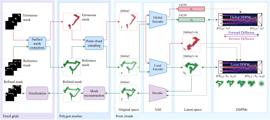
Figure 2: Latent conditional point cloud refinement framework: surface meshes are extracted from the reference and erroneous organ masks using the marching cubes algorithm and point clouds are sampled from both surfaces using Poisson disk sampling. The shapes are encoded into a global and a local representation via two VAE encoders. Two DDPMs are trained to model the distributions of global and local representations of the complete shapes conditioned on the partial shapes’ latent representations. The clean shape is reconstructed to the original space via the VAE’s decoder. After post-processing, Point-E’s deep implicit model is used to reconstruct a polygon mesh that can be voxelized into a 3D mask.

2.3 Baseline: Conditional Generation Network

As a first step, we trained the Conditional Generative Network (CGNet) of PDR[25] on our dataset which later served as our baseline. Assuming $p_{intestine}$ is the distribution of the complete large intestine shapes $x^{i}$ and $p_{latent}$ is the latent distribution representing a standard Gaussian in $\mathbb{R}^{N\times 3}$, CGNet is designed as a DDPM that consists of two processes:

• The forward diffusion process: a Markov chain that adds noise gradually to the clean data distribution $p_{intestine}$ using Gaussian kernels of fixed variances in T time steps. Variances are fixed such that at the final step T, the shapes belong to the standard Gaussian distribution $p_{latent}$. This process does not depend on the conditioner.

• The reverse diffusion process: a Markov chain implemented as a neural network based on an encoder-decoder architecture with PointNet++[26] backbone. The model predicts the noise added during the forward process. This process is conditioned on the erroneous shape $c$. It starts with a sample $x_{T}$ from $p_{latent}$ and gradually denoises it to obtain a clean shape $x_{0}$ from $p_{intestine}$.

To make the model work on our dataset we introduced some modifications to the default hyper-parameters provided by PDR’s authors. We used a time embedding of size 128. The depths of all MLPs in the decoders were increased to 3 and the number of neighbors K used for clustering in all PointNet++ layers was set to 10. The number of features of the conditioner (other than the xyz-coordinates) was set to 0. Since we are only training on a single class, the class conditioning mechanism was removed. We trained the model for 8000 epochs with a learning rate of $5\times 10^{-4}$ and a batch size of 16.

2.4 Latent Conditional Point-Diffusion Network

To improve the refinement performance, we propose to shift the conditional generation process to a smoother latent space. The inspiration behind this lies in the high complexity and variability of the large intestine’s shapes, making it challenging for the DDPM to accurately model their distribution in the original space. Inspired by Zeng et al. [24], we propose to train a VAE that encodes both partial and complete shapes into a unified smoother latent space consisting of a vector-valued global representation and a point cloud-structured local representation. Subsequently, two DDPMs were trained to model the distributions of complete shapes’ latent representations conditioned on the representations of partial shapes. This enables the disentanglement of high-level features related to the overall appearance of the organ from the low-level features expressing the fine details, making it easier for the DDPMs to model the underlying distributions. Finally, the VAE’s decoder was used to combine both representations to reconstruct the complete shape in the original space. The overall design of our complete framework is illustrated in Fig. 2.

2.4.1 Hierarchical Latent Shape Encoding

For the latent shape encoding, we adapted the approach proposed by Zeng et al.[24]. Taking a pair of shapes (x, c) from the training set $\mathcal{D}$, a VAE learns a global latent representation $(z_{x},z_{c})\in(\mathbb{R}^{D_{z}})^{2}$ and a local latent representation $(h_{x},h_{c})\in(\mathbb{R}^{N\times(3+D_{h})})^{2}$. In other words, $z_{x}$ and $z_{c}$ are 1D vectors of size $D_{z}$ whereas $h_{x}$ and $h_{c}$ are latent point clouds of N points, each carrying its xyz-coordinates and $D_{h}$ additional features. The VAE consisted of two encoders and a decoder all based on the PVCNN architecture [31]. The global encoder takes a 3D point cloud $s\in\{x,c\}$ as input and encodes it into a global latent vector $z_{s}$. The local encoder takes the point cloud s as input and its global representation $z_{s}$ as a condition and generates the corresponding local representation $h_{s}$. The VAE’s decoder takes $h_{s}$ as input and $z_{s}$ as a condition and reconstructs the shape s back to the original space. The VAE was trained by maximizing a modified version of the variational lower bound on the data log-likelihood (ELBO)[24].

We fine-tuned the default hyperparameters provided by zeng et al.[24] according to our use case. We set $D_{z}$ to 256 and $D_{h}$ to 4. The maximum values of both KL weights of the loss function $\lambda_{z}$ and $\lambda_{h}$ were set to 0.4. To initialize the VAE weights, the variance offset parameter was set to 12 and the skip connections’ weight was set to 0.02. We trained the model using Adam optimizer with a batch size of 32 and a learning rate of $10^{-3}$ for 8000 epochs while saving the weights every 2000 epochs. Note that the VAE was trained using both partial and complete shapes since both shapes need to be encoded to the latent space for training the conditional DDPMs.

2.4.2 Latent Conditional Point Generation

Using the VAE weights saved at epoch 6000 (the selection is justified in section 3.4.1), we trained two conditional DDPMs in the hierarchical latent space. A first DDPM with parameters $\xi$ was trained on the global latent encodings $z_{x}$ conditioned on $z_{c}$. A second DDPM with parameters $\phi$ was trained on the local latent encodings $h_{x}$ conditioned on both $h_{c}$ and $z_{x}$. The models were trained by minimizing the difference between the actual noise added to the reference latent encodings and the noise predicted by the DDPMs. The loss function of the first DDPM can be written as:

$$\mathcal{L}(\xi)=\mathbb{E}_{i\sim\mathcal{U}([M]),t\sim\mathcal{U}([T]),\epsilon\sim\mathcal{N}(0,I)}\left\|\epsilon-\epsilon_{\xi}(z_{x,t}^{i},t,z_{c}^{i})\right\|^{2}$$ (1)

where $\mathcal{U}([M])$ represents the uniform distribution over {1, 2,…,M}, $\mathcal{U}([T])$ represents the uniform distribution over {1, 2,…,T}, $z_{x,t}^{i}$ is the diffused global latent representation of the shape $x^{i}$ after t diffusion steps, $z_{c}^{i}$ is the global representation of the corresponding conditioner $c^{i}$, $\epsilon$ is the actual noise and $\epsilon_{\xi}$ is the noise predicted by the model.
Similarly, the loss function of the second DDPM is defined as:

$$\mathcal{L}(\phi)=\mathbb{E}_{i\sim\mathcal{U}([M]),t\sim\mathcal{U}([T]),\epsilon\sim\mathcal{N}(0,I)}\left\|\epsilon-\epsilon_{\phi}(h_{x,t}^{i},t,h_{c}^{i},z_{x,0}^{i})\right\|^{2}$$ (2)

where $h_{x,t}^{i}$ is the diffused local latent representation of the shape $x^{i}$ after t diffusion steps, $h_{c}^{i}$ is the local representation of the corresponding conditioner $c^{i}$, $z_{x,0}^{i}$ is the clean global representation of $x^{i}$, $\epsilon$ is the actual noise and $\epsilon_{\phi}$ is the noise predicted by the model. The fixed diffusion variances are defined using a linear scheduler for both models. Note that during this process, the latent encodings of the conditioner $(z_{c},h_{c})$ are only used to extract features that are embedded into the diffusion models to guide the denoising process and they are not diffused. The global DDPM was implemented as a ResNet with 8 squeeze-and-excitation blocks whereas the local DDPM used the same architecture as the CGNet without the additional PointNet used for extracting global features. Instead, the global representation of the complete shape generated by the global DDPM was used as global features.

We used a 256-dimensional time embedding and 1000 diffusion steps in both models. We set the dropout of the ResNet layers to 0.2. Different from the baseline CGNet, the ReLU activation function is replaced by Swish[32]. Based on the feature size of our local latent representations, the number of the partial input features was set to 4 and the feature dimension of the output was set to 7. The DDPMs were trained in parallel using Adam optimizer with a batch size of 10 and a learning rate of $2\times 10^{-4}$ for 16000 epochs.

At inference, the erroneous shape c is encoded into its latent representations $(z_{c},h_{c})$, and two noisy inputs $z_{x,T}$ and $h_{x,T}$ are sampled from a normal Gaussian distribution. First, the reverse diffusion process is performed on $z_{x,T}$ using the global DDPM to obtain a clean global representation $z_{x,0}$. Later, the local DDPM is used to run the reverse diffusion process on $h_{x,T}$ to obtain a clean local representation $h_{x,0}$ using both $h_{c}$ and the generated $z_{x,0}$ as conditions. Finally, the resulting representations are decoded back to the original space via the VAE’s decoder.

2.5 Point Cloud Post-Processing

The output of the generative model tends to be sparse and noisy which effects negatively the performance of the surface reconstruction. To address this issue we propose a simple point cloud post-processing pipeline consisting of the following steps:

• The point cloud is first renormalized back to the original scale.

• The cloud is smoothed using a variant of the Moving Least Square algorithm with a smoothing factor of 0.2.

• The cloud is densified by adding new points under the assumption that all points in a local neighborhood are within a specified distance of each other. If any neighbor exceeds the target distance, the connecting edge is divided and a new point is inserted at the midpoint. We use a target distance of 10 mm and a neighborhood size of 10 points. We apply this process for one iteration.

• Outlier removal is applied such that all points having less than 5 neighbors within a radius of 15 mm are removed.

2.6 Surface Reconstruction

Since the goal is to generate organs for computational phantoms that are usually represented as polygon meshes, we extended our method with a deep implicit model for point-cloud-to-mesh reconstruction (pc2mesh) proposed within the Point-E framework[33]. This model uses an encoder-decoder Transformer architecture and predicts SDFs based on the input point clouds. The mesh is obtained by applying the marching cubes algorithm on the generated SDF map. In our experiments, we used the provided pre-trained weights and a grid size of $128\times 128\times 128$ with a batch size of 1024 points. Point clouds were normalized to [-0.5, 0.5] before being fed to the model.

3 Results

To evaluate the shape refinement performance, we relied on three main evaluation metrics: Chamfer distance (CD), Hausdorff distance (HD) and Earth Mover distance (EMD). These metrics collectively enable the assessment of completeness, geometric accuracy, and distribution fidelity between the generated point clouds and the reference shapes.

3.1 Point Cloud Refinement

After running the inference pipeline using both CGNet and our proposed latent conditional point diffusion model on our synthetic test set, we summarize the results of point cloud refinement obtained in terms of CD, HD, and EMD in table 2. We also report the metrics obtained initially between the complete and the erroneous shapes used as model conditions for reference. Fig 3 shows examples of refined large intestine point clouds using both models.

[5pt]

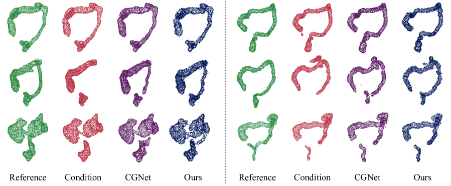
Figure 3: Examples of the shape refinement results

Model	CD $\downarrow$	HD $\downarrow$	EMD $\downarrow$
Init	1396 $\pm$ 2615	84.01 $\pm$ 59	9430 $\pm$ 7150
CGNet	449 $\pm$ 853	57.18 $\pm$ 32	9294 $\pm$ 4940
Ours	388 $\pm$ 681	56.44 $\pm$ 31	9666 $\pm$ 4855

Table 2: Shape refinement results on the test set.

Both CGNet and our latent conditional point-diffusion model show significant improvements in surface reconstruction compared to the starting point. Our model outperforms CGNet with a 13.95% improvement in CD and 1.29% in HD on average, indicating better handling of local errors and improved alignment with reference shapes. However, CGNet performs better than our model in terms of EMD, indicating that our shapes exhibit lower visual quality and less uniform density. Additionally, our proposed method demonstrates reduced dispersion, leading to higher stability, as indicated by lower standard deviation for all metrics. Our method accurately captures the overall distribution of large intestine shapes, producing anatomically acceptable results. It effectively completes missing parts and eliminates false positives in certain scenarios. However, shapes generated by the latent model are noisier and sparser compared to CGNet, resulting in higher EMD values. Additionally, the model faces challenges in removing adjacent or attached false positives but often combines them with correct segments, creating a more plausible connected representation of the large intestine. Occasionally, the model fails to connect organ segments.

The visual quality improvement in our model compared to CGNet is noticeable, but the average differences in HD and EMD are not statistically significant. Further inspection of individual cases such as the examples in fig. 4 revealed that critical cases with relatively larger defects compared to the organ’s size show more significant metric improvement and model differences, while cases with smaller local defects have a smaller impact on the average metrics. This observation suggests that the average metrics are influenced by cases with smaller local defects, which are more prevalent in our test set.

[5pt]

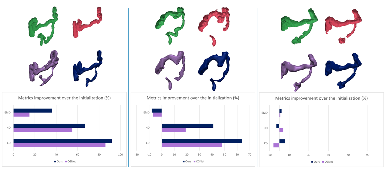
Figure 4: Refinement results for individual cases with the corresponding improvement in the metrics (HD, CD and EMD) over the initialization showing that the difference is larger for cases with larger defects (Left and Middle) compared to cases with small defects (Right).

3.2 Surface Reconstruction

The generated point clouds of both CGNet and our model were post-processed using the pipeline proposed in section 2.5 then given as input to Point-E’s pc2mesh model to generate the polygon meshes. To evaluate the performance, we sampled 50000 points from the mesh surfaces and computed CD, HD, and EMD between the generated and the reference meshes. The results are summarized in table 3. Examples of the post-processed point clouds and the corresponding reconstructed meshes are shown in Fig. 5.

[5pt]

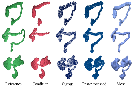
Figure 5: Example results of post-processed point clouds and the corresponding reconstructed meshes.

Model	CD $\downarrow$	HD $\downarrow$	EMD $\downarrow$
Init	1400 $\pm$ 2620	84.22 $\pm$ 58	9767 $\pm$ 6995
CGNet	463 $\pm$ 871	57.13 $\pm$ 32	9273 $\pm$ 4950
Ours	409 $\pm$ 716	56.43 $\pm$ 31	9096 $\pm$ 4836

Table 3: Shape refinement results after surface reconstruction.

After applying post-processing and surface reconstruction, our method maintains high performance across all metrics. Notably, our model outperforms CGNet in all metrics, including EMD, indicating the effectiveness of our post-processing and mesh reconstruction pipeline in reducing the noise and sparsity of the generated shapes. This highlights the ability of our pipeline in modeling the distribution of the large intestine’s shape in terms of global appearance, local details, and density uniformity. Additionally, visual inspection reveals that the post-processed point clouds exhibit smoother and denser characteristics compared to the raw ones. The reconstructed meshes exhibit high quality and preserve fine details. In fact, they are less affected by discretization compared to the reference meshes generated from the binary segmentation masks.

3.3 TotalSegmentator Refinement

After testing our proposed pipeline on synthetic data, we evaluated its real-world performance using 20 CT scans (8 CAP and 12 PET/CT). The large intestine segmentation masks were obtained using TotalSegmentator, then refined by a physician to create the reference masks. Both the CGNet and our latent conditional point diffusion model were then applied on the model’s results. The refinement results compared to the reference meshes are in Table 4; visual examples are in 6.

Model	CD $\downarrow$	HD $\downarrow$	EMD $\downarrow$
TotalSeg	571 $\pm$ 929	93.97 $\pm$ 137	6916 $\pm$ 3766
TotalSeg+CGNet	313 $\pm$ 543	74.81 $\pm$ 131	8432 $\pm$ 4543
TotalSeg+Ours	230 $\pm$ 346	72.46 $\pm$ 132	7893 $\pm$ 3144

Table 4: Shape refinement results on TotalSegmentator cases

[5pt]

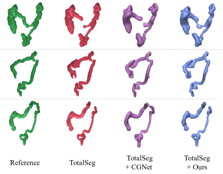
Figure 6: Examples of TotalSegmentator outputs and their refinement results

The results demonstrate significant improvement of the proposed method in refining the large intestine’s surface compared to the segmentation results of TotalSegmentator. On average, we achieved a 62.32% improvement in CD and a 2.15% improvement in HD, outperforming CGNet in both metrics. However, it is worth noting that both our proposed method and CGNet exhibit poor EMD results compared to TotalSegmentator, although our model still outperforms CGNet in this metric. The qualitative evaluation confirms that the observations made on the synthetic set (accurate distribution modeling, noise elimination in certain cases, and failure scenarios) are consistent with real-world cases.

3.4 Ablation Study

3.4.1 Latent Space Smoothness Impact

During VAE training, the KL divergence weights of the loss function are gradually increased, leading the latents $p(z_{s})$ and $p(h_{s})$ to converge towards a standard Gaussian. This results in smoother and more regular latent spaces but increases reconstruction error. To evaluate the impact of VAE weights on the generation process, three latent DDPMs (A, B, and C) were trained using the VAE weights saved at epochs 4000, 6000, and 8000, respectively. Generation metrics on raw point clouds are presented in Table 5, and example shapes generated using the different models are shown in Fig 7.

The model trained with VAE weights from epoch 6000 outperformed the others in terms of both CD and EMD, while the model trained with weights from epoch 8000 achieved the lowest HD. Qualitative evaluation showed that extending VAE training time (smoothing the latent space) improved the shape distribution modeling, resulting in more compact and connected organs. However, the reconstruction quality decreased, leading to noisier shapes. Overall, using VAE weights from epoch 6000 balances the trade-off between latent space smoothness and the reconstruction performance.”

Model	CD $\downarrow$	HD $\downarrow$	EMD $\downarrow$
A	422 $\pm$ 847	55.99 $\pm$ 32	10231 $\pm$ 4913
B	388 $\pm$ 681	56.44 $\pm$ 31	9666 $\pm$ 4855
C	411 $\pm$ 821	54.25 $\pm$32	9972$\pm$ 4975

Table 5: Experimental results on latent space smoothness impact on the generated organ point clouds.

[5pt]

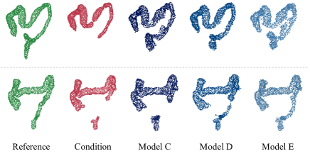
Figure 7: Examples illustrating the impact of latent space smoothness on the generated organ point clouds.

3.4.2 Post-processing

To assess the impact of the proposed post-processing pipeline, we generated meshes using both the raw and the post-processed point clouds and we report the results we obtained in table 6. Examples of the generated meshes from the raw and post-processed clouds are illustrated in Fig 8.

Post-process	CD $\downarrow$	HD $\downarrow$	EMD $\downarrow$
Before	427 $\pm$ 837	54.07 $\pm$ 32	9344 $\pm$ 4914
After	431 $\pm$ 849	54.05 $\pm$ 32	9253 $\pm$ 5032

Table 6: Mesh reconstruction results before and after post-processing.

[5pt]

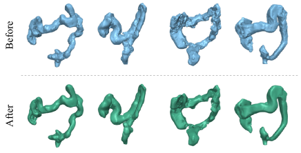
Figure 8: Examples illustrating the impact of post-processing on the reconstructed meshes.

While the performance metrics do not exhibit a substantial difference, the qualitative evaluation highlights the benefits of post-processing. The meshes generated after post-processing are smoother and suffer fewer holes and noise along their surfaces, which is more compatible with the anatomy of the large intestine’s walls primarily consisting of soft tissues.

3.4.3 Data Augmentation

To address the problem of small dataset size with respect to the complexity of the shapes, we implemented a simple data augmentation pipeline based on rigid 3D transformations. We use a scaling factor of up to 10% of the original size, a rotation around the z-axis of up to 10°, and a translation of up to 0.1 units in the normalized space. We apply this pipeline to train both the VAE and DDPMs of a new model (Ours-Aug). The quantitative results computed from the generated point clouds are represented in table 7. Figure 9 illustrates examples generated using this model.

Model	CD $\downarrow$	HD $\downarrow$	EMD $\downarrow$
Ours-Aug	449 $\pm$ 814	54.62 $\pm$ 32	11019 $\pm$ 4874

Table 7: Shape refinement results of the model trained with data augmentation

[5pt]

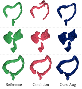
Figure 9: Example shapes generated by the model trained with data augmentation.

Compared to models without data augmentation, this model improves on various issues, reducing false positives and closely matching reference shapes, leading to minimized HD. However, the generated shapes exhibit more dispersion and noise, introducing new errors like links between the cecum and rectosigmoid junction, resulting in higher EMD and CD values.

4 Discussion

In this study, we investigated the application of geometric deep learning techniques and denoising diffusion models to refine erroneous segmentation masks of the large intestine. These masks were generated by a volumetric segmentation model and exhibit multiple issues such as missing parts or noise. We approached the problem as a conditional point cloud generation task and proposed a latent conditional point diffusion model for point cloud refinement. Our pipeline involves sampling point clouds from the organ’s surfaces and encoding the shapes into a smoother latent space consisting of a global and a local representation using a hierarchical VAE’s encoder. Two DDPMs are then trained in this latent space to perform point cloud refinement. The generated latent point clouds are then decoded back to the original space using the VAE’s decoder before being post-processed. Finally, a surface mesh is reconstructed using a modern deep implicit model.

By comparing our proposed method to CGNet, we observed that training the DDPMs in a hierarchical latent space yields significant advantages in modeling shape distributions, particularly in capturing fine details. Our method demonstrates superior local performance by effectively handling the false positives, while CGNet tends to produce anatomically inaccurate details, such as including small branches in some sections of the colon. Our conclusions were reinforced by the study on the impact of latent space smoothness, which showed that models trained in smoother spaces better preserved the organ’s anatomy. However, it’s important to note that CGNet generated denser and more uniform point clouds compared to the latent model which tended to generate noisier and sparser point clouds. This phenomenon is attributed to the encoding and decoding process between the original and latent spaces. Our proposed post-processing and mesh reconstruction methods effectively resolved this issue, producing high-quality meshes with detailed structures and minimal noise. Further fine-tuning of the post-processing parameters could enhance the shape quality.

Unlike [18] who suggests using a point classification network to eliminate background points in the segmentation result, our method utilizes generative deep learning. This enabled our model to generate new parts and complete partial and disconnected shapes obtained from the segmentation model. [27], on the other hand, adopted PVD’s architecture[23] for generating skull implants. Their method assumes that the conditioner is entirely contained within the target shape and maintains it fixed throughout the diffusion process. However, in our case, the conditioner may contain noise and fragments of other organs, rendering the use of such techniques impractical since the false positive points will still be present in the output. To overcome this issue, we employed the CGNet architecture introduced by [25]. Unlike the model used in PVD, CGNet does not fix the partial shape but rather extracts its features to guide the generation process. By adopting this strategy, our model successfully eliminated noisy components from the masks in several cases.

We applied our pipeline to outputs generated by TotalSegmentator, a well-known model that was trained on one of the largest imaging datasets. Compared to the corresponding masks refined by a physician, we noticed a significant improvement in the surface representation performance. Additionally, the qualitative evaluation showed consistency with the results obtained on our test set indicating the faithfulness of our synthetic dataset to the actual outputs of the model and the generalizability of our model to new cases. On the other hand, the model resulted in higher EMD values compared to TotalSegmentator’s output. Besides model failures, this observation can be attributed to several factors. For instance, the cases included in this set suffered mostly from local problems such as disconnections or small parts included from the other organs and EMD does not quantify well local dissimilarity.

4.1 Limitations

While our method shows promising results for large intestine segmentation refinement, it does have limitations. The model struggles to eliminate false positives closely adjacent or attached to the actual segments of the organ. PointNet’s layers classify these points as neighbors of nearby true positives, causing their inclusion in clusters and contributing to the generation process. Additionally, the model struggles with connecting segments in the large intestine, especially near the rectosigmoid junction, and may produce anatomically inaccurate shapes for complex or multi-curved inputs. Increasing the training set size can address these issues. Moreover, the generated shapes sometimes misalign with the ground truth, intersecting neighboring organs and preventing the 3D model from fitting in the computerized phantom. This occurs because the current model relies only on the provided partial shape, lacking essential contextual information about surrounding organs.

4.2 Future Work

To improve our model, we propose the following steps: (1) Further engineering of the neighborhood definition hyperparameters and attention modules in the CGNet model to better distinguish between true and false positives. (2) Increasing data diversity by acquiring more scans and optimizing the data augmentation parameters. (3) Exploring the use of neighboring organs’ landmarks as a second condition for the generative models to avoid intersections and improve shape accuracy. (4) An optimized landmarks extraction technique and a more comprehensive test set can lead to a generalized generation approach where new organs can be generated from scratch without the need for a segmentation algorithm (5) Enhancing mesh reconstruction by fine-tuning the Point-E model on our data or modifying the VAE decoder to output signed distance functions. Implementing these solutions will boost the model’s performance in eliminating false positives, diversifying the dataset, and improving mesh reconstruction quality.

5 Conclusions

We have presented an end-to-end automatic pipeline for refining 3D shapes of the large intestine, which improves the surface reconstruction of the organ starting from an erroneous segmentation. Our method is based on geometric deep learning and denoising diffusion probabilistic models. We formulate the refinement process as a conditional point cloud generation problem performed in a hierarchical latent space. Through a comprehensive evaluation of the method on the test set, our approach has demonstrated promising results both quantitatively and qualitatively. The refined 3D shapes exhibited improved surface reconstruction and enhanced anatomical accuracy compared to the outputs of the segmentation model. This study validates the effectiveness of utilizing geometric DL and DDPMs in enhancing the surface reconstruction of deformable anatomical structures, using the large intestine as an example.

Our method opens up possibilities for further improvement and can be extended to multiple applications that could enhance the quality of computerized phantoms. Future work includes incorporating additional contextual information from neighboring structures to restrict the generation region and expanding the model to perform label-aware refinement of multiple organs.

6 References

References

- [1] W. Segars, J. Bond, J. Frush, S. Hon, C. Eckersley, C. H. Williams, J. Feng, D. J. Tward, J. Ratnanather, M. Miller et al., “Population of anatomically variable 4d xcat adult phantoms for imaging research and optimization,” Medical physics, vol. 40, no. 4, p. 043701, 2013.
- [2] J. Y. Hesterman, S. D. Kost, R. W. Holt, H. Dobson, A. Verma, and P. D. Mozley, “Three-dimensional dosimetry for radiation safety estimates from intrathecal administration,” Journal of Nuclear Medicine, vol. 58, no. 10, pp. 1672–1678, 2017.
- [3] M. Wang, N. Guo, G. Hu, G. El Fakhri, H. Zhang, and Q. Li, “A novel approach to assess the treatment response using gaussian random field in pet,” Medical Physics, vol. 43, no. 2, pp. 833–842, 2016.
- [4] W. P. Segars, G. Sturgeon, S. Mendonca, J. Grimes, and B. M. Tsui, “4d xcat phantom for multimodality imaging research,” Medical physics, vol. 37, no. 9, pp. 4902–4915, 2010.
- [5] C. Lee, D. Lodwick, D. Hasenauer, J. L. Williams, C. Lee, and W. E. Bolch, “Hybrid computational phantoms of the male and female newborn patient: Nurbs-based whole-body models,” Physics in Medicine & Biology, vol. 52, no. 12, p. 3309, 2007.
- [6] Y. Liu, Y. Lei, Y. Fu, T. Wang, X. Tang, X. Jiang, W. J. Curran, T. Liu, P. Patel, and X. Yang, “Ct-based multi-organ segmentation using a 3d self-attention u-net network for pancreatic radiotherapy,” Medical physics, vol. 47, no. 9, pp. 4316–4324, 2020.
- [7] A. D. Weston, P. Korfiatis, K. A. Philbrick, G. M. Conte, P. Kostandy, T. Sakinis, A. Zeinoddini, A. Boonrod, M. Moynagh, N. Takahashi et al., “Complete abdomen and pelvis segmentation using u-net variant architecture,” Medical physics, vol. 47, no. 11, pp. 5609–5618, 2020.
- [8] J. Wasserthal, M. Meyer, H.-C. Breit, J. Cyriac, S. Yang, and M. Segeroth, “Totalsegmentator: robust segmentation of 104 anatomical structures in ct images,” arXiv preprint arXiv:2208.05868, 2022.
- [9] J. J. Cerrolaza, M. L. Picazo, L. Humbert, Y. Sato, D. Rueckert, M. Á. G. Ballester, and M. G. Linguraru, “Computational anatomy for multi-organ analysis in medical imaging: A review,” Medical image analysis, vol. 56, pp. 44–67, 2019.
- [10] C. Wang, Z. Cui, J. Yang, M. Han, G. Carneiro, and D. Shen, “Bowelnet: Joint semantic-geometric ensemble learning for bowel segmentation from both partially and fully labeled ct images,” IEEE Transactions on Medical Imaging, 2022.
- [11] O. Ronneberger, P. Fischer, and T. Brox, “U-net: Convolutional networks for biomedical image segmentation,” in Medical Image Computing and Computer-Assisted Intervention–MICCAI 2015: 18th International Conference, Munich, Germany, October 5-9, 2015, Proceedings, Part III 18. Springer, 2015, pp. 234–241.
- [12] J. Yang, U. Wickramasinghe, B. Ni, and P. Fua, “Implicitatlas: learning deformable shape templates in medical imaging,” in Proceedings of the IEEE/CVF Conference on Computer Vision and Pattern Recognition, 2022, pp. 15 861–15 871.
- [13] A. Raju, S. Miao, D. Jin, L. Lu, J. Huang, and A. P. Harrison, “Deep implicit statistical shape models for 3d medical image delineation,” in Proceedings of the AAAI Conference on Artificial Intelligence, vol. 36, no. 2, 2022, pp. 2135–2143.
- [14] L. Bai, Y. Zhao, M. Elhousni, and X. Huang, “Depthnet: Real-time lidar point cloud depth completion for autonomous vehicles,” IEEE Access, vol. 8, pp. 227 825–227 833, 2020.
- [15] J. Varley, C. DeChant, A. Richardson, J. Ruales, and P. Allen, “Shape completion enabled robotic grasping,” in 2017 IEEE/RSJ international conference on intelligent robots and systems (IROS). IEEE, 2017, pp. 2442–2447.
- [16] C. R. Qi, H. Su, K. Mo, and L. J. Guibas, “Pointnet: Deep learning on point sets for 3d classification and segmentation,” in Proceedings of the IEEE conference on computer vision and pattern recognition, 2017, pp. 652–660.
- [17] A. Jana, H. M. Subhash, and D. Metaxas, “Automatic tooth segmentation from 3d dental model using deep learning: a quantitative analysis of what can be learnt from a single 3d dental model,” in 18th International Symposium on Medical Information Processing and Analysis, vol. 12567. SPIE, 2023, pp. 42–51.
- [18] F. Balsiger, Y. Soom, O. Scheidegger, and M. Reyes, “Learning shape representation on sparse point clouds for volumetric image segmentation,” in Medical Image Computing and Computer Assisted Intervention–MICCAI 2019: 22nd International Conference, Shenzhen, China, October 13–17, 2019, Proceedings, Part II 22. Springer, 2019, pp. 273–281.
- [19] Y. Li, R. Bu, M. Sun, W. Wu, X. Di, and B. Chen, “Pointcnn: Convolution on x-transformed points,” Advances in neural information processing systems, vol. 31, 2018.
- [20] J. Ho, A. Jain, and P. Abbeel, “Denoising diffusion probabilistic models,” Advances in Neural Information Processing Systems, vol. 33, pp. 6840–6851, 2020.
- [21] J. Zhang, S. Jayasuriya, and V. Berisha, “Restoring degraded speech via a modified diffusion model,” arXiv preprint arXiv:2104.11347, 2021.
- [22] A. Lugmayr, M. Danelljan, A. Romero, F. Yu, R. Timofte, and L. Van Gool, “Repaint: Inpainting using denoising diffusion probabilistic models,” in Proceedings of the IEEE/CVF Conference on Computer Vision and Pattern Recognition, 2022, pp. 11 461–11 471.
- [23] L. Zhou, Y. Du, and J. Wu, “3d shape generation and completion through point-voxel diffusion,” in Proceedings of the IEEE/CVF International Conference on Computer Vision, 2021, pp. 5826–5835.
- [24] X. Zeng, A. Vahdat, F. Williams, Z. Gojcic, O. Litany, S. Fidler, and K. Kreis, “Lion: Latent point diffusion models for 3d shape generation,” in Advances in Neural Information Processing Systems, 2022.
- [25] Z. Lyu, Z. Kong, X. Xu, L. Pan, and D. Lin, “A conditional point diffusion-refinement paradigm for 3d point cloud completion,” arXiv preprint arXiv:2112.03530, 2021.
- [26] C. R. Qi, L. Yi, H. Su, and L. J. Guibas, “Pointnet++: Deep hierarchical feature learning on point sets in a metric space,” Advances in neural information processing systems, vol. 30, 2017.
- [27] P. Friedrich, J. Wolleb, F. Bieder, F. M. Thieringer, and P. C. Cattin, “Point cloud diffusion models for automatic implant generation,” arXiv preprint arXiv:2303.08061, 2023.
- [28] F. Isensee, P. F. Jaeger, S. A. Kohl, J. Petersen, and K. H. Maier-Hein, “nnu-net: a self-configuring method for deep learning-based biomedical image segmentation,” Nature methods, vol. 18, no. 2, pp. 203–211, 2021.
- [29] W. E. Lorensen and H. E. Cline, “Marching cubes: A high resolution 3d surface construction algorithm,” ACM siggraph computer graphics, vol. 21, no. 4, pp. 163–169, 1987.
- [30] C. Yuksel, “Sample elimination for generating poisson disk sample sets,” in Computer Graphics Forum, vol. 34, no. 2. Wiley Online Library, 2015, pp. 25–32.
- [31] Z. Liu, H. Tang, Y. Lin, and S. Han, “Point-voxel cnn for efficient 3d deep learning,” Advances in Neural Information Processing Systems, vol. 32, 2019.
- [32] P. Ramachandran, B. Zoph, and Q. V. Le, “Searching for activation functions,” arXiv preprint arXiv:1710.05941, 2017.
- [33] A. Nichol, H. Jun, P. Dhariwal, P. Mishkin, and M. Chen, “Point-e: A system for generating 3d point clouds from complex prompts,” arXiv preprint arXiv:2212.08751, 2022.