UNSUPERVISED DISENTANGLING OF FACIAL REPRESENTATIONS WITH 3D-AWARE LATENT DIFFUSION MODELS

Abstract

Unsupervised learning of facial representations has gained increasing attention for face understanding ability without heavily relying on large-scale annotated datasets. However, it remains unsolved due to the coupling of facial identities, expressions, and external factors like pose and light. Prior methods primarily focus on 2D factors and pixel-level consistency, leading to incomplete disentangling and suboptimal performance in downstream tasks. In this paper, we propose LatentFace, a novel unsupervised disentangling framework for facial expression and identity representation. We suggest the disentangling problem should be performed in latent space and propose the solution using a 3D-aware latent diffusion model. First, we introduce a 3D-aware autoencoder to encode face images into 3D latent embeddings. Second, we propose a novel representation diffusion model (RDM) to disentangle 3D latent into facial identity and expression. Consequently, our method achieves state-of-the-art performance in facial expression recognition and face verification among unsupervised facial representation learning models. Codes are available at https://github.com/ryanhe312/LatentFace.

Index Terms—  facial representation, 3D, unsupervised learning, diffusion models

1 Introduction

Human faces hold significant importance in the field of computer vision, serving as carriers of vital information, including identity, expressions, and intentions [1]. Recent advancements in neural networks have led to remarkable achievements in facial understanding [2, 3]. Nonetheless, supervised learning requires large-scale annotated datasets and faces challenges such as imbalance annotation [4, 5] and the labor-intensive labeling work [6]. In response, unsupervised learning methods have been proposed to tackle this issue by focusing on learning facial representations rather than directly predicting labels.

Recent image representation learning methods, such as contrastive learning [7] and masked autoencoders [8], have garnered considerable interest. These models are unsupervisedly trained on unlabeled datasets to acquire implicit representations. Nevertheless, these representations lack interpretability and fail to account for the semantic and structural aspects of the human face.

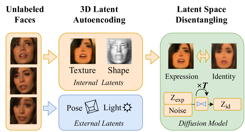
Fig. 1: Our framework can disentangle facial expression and identity representations from unlabeled face images.

To leverage the face structure, disentangling is a common practice for learning facial representations. The approach is to distinguish facial expression and identity from changing environments. Prior methods [9, 10, 11, 12] have achieved good results in learning facial factors in 2D space. However, there are two problems with facial representation disentangling. First, previous techniques exhibit limitations in terms of 3D awareness and have subpar performance when there is drastic light and pose variations of face images. Second, they focus on pixel-level warping [9, 11], leading to the incomplete disentanglement of facial representations. Our contributions to address the problems are three-fold:

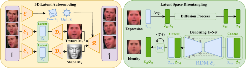
Fig. 2: Overview of the proposed unsupervised learning framework. In the first stage, we disentangle 3D factors, including texture, shape, pose, and light, through the training of autoencoders (comprising encoders $\mathcal{E}$ and decoders $\mathcal{D}$) and render them using a renderer $\mathcal{R}$ to reconstruct the input. In the second stage, we further disentangle the texture and shape latent and train the Representation Diffusion Model (RDM) $\mathcal{E}{r}$ to generate the identity latent $Z_{id}$ from the emotional face latent $Z_{exp}$.

First, we propose LatentFace, a novel unsupervised disentangling framework for facial expression and identity representations. We suggest that the disentangling problem be performed in latent space. To the best of our knowledge, we propose the first 3D-aware latent diffusion model for unsupervised facial representation learning.

Second, we propose a 3D-aware autoencoder and a Representation Diffusion Model (RDM). As illustrated in Fig. 1, the 3D-aware autoencoder disentangles light and pose and encodes facial shape and texture from face images. Then, RDM disentangles facial identity from expressions based on extracted shape and texture embedding.

Third, extensive experiments have demonstrated that our model achieves state-of-the-art performance on unsupervised facial expression recognition (FER) and face verification. Specifically, our model has a 4.5% advantage in FER accuracy on RAF-DB [13] and 3.4% on AffectNet [14] compared to SOTA unsupervised methods.

2 Methodology

2.1 Overview

Given a face image $I$, the representation learning models are expected to encode the image as latent embeddings, denoted as $Z$. As illustrated in Fig. 2, our proposed unsupervised learning framework learns facial expression and identity embeddings from unlabeled images and videos. Our framework comprises two stages: 3D latent autoencoding and latent space disentangling.

2.2 3D Latent Autoencoding

The first stage of our approach is dedicated to learning 3D facial latent embeddings, including pose $Z_{p}$, light $Z_{l}$, facial texture $Z_{t}$, and shape $Z_{s}$. Leveraging the ample variations in facial and external factors found in image sets [15], the model learns to disentangle them with an autoencoder. We follow Unsup3D [16] to model the face as an unsupervised non-linear parametric model of texture and shape. The facial representations are learned through a self-supervised scheme, which uses the minimal assumption of face symmetry to make the problem converge to stereo reconstruction.

Specifically, the texture and shape of 3D face model are learned by encoders $\mathcal{E}$ and decoder $\mathcal{D}$ with the equation $M=\mathcal{D}(Z)=\mathcal{D}(\mathcal{E}(I))$. In contrast, the light and pose are predicted directly from encoders with the equation $Z=\mathcal{E}(I)$. Finally, the model reconstructs the input face $I$ by rendering the extracted features and the flipped feature map:

$$\hat{I} =\mathcal{R}(M_{t},M_{s},Z_{p},Z_{l}),$$ (1)

$$\hat{I}^{\prime} =\mathcal{R}(\text{flip}(M_{t}),\text{flip}(M_{s}),Z_{p},Z_{l}),$$ (2)

where $M_{s}$ is the facial shape and $M_{t}$ is the facial texture. $Z_{l}$ is the light color and direction, and $Z_{p}$ is the camera’s pose. $\text{flip}(\cdot)$ is a horizontal flip operator. $\hat{I}$ is the reconstructed face, and $\hat{I}^{\prime}$ is the symmetric face generated from the flipped feature map. For the renderer $\mathcal{R}$, we implement a differentiable rendering pipeline with a diffuse illumination model and a weak perspective camera using Pytorch3D.

Method	Aff-wild2	RAF-DB	AffectNet	Pose 30∘	Pose 45∘	LFW	SLLFW
SimCLR[7]	38.69/25.94	64.47/47.48	40.15/38.86	37.69/36.57	37.84/37.41	63.38$\pm$2.13	51.18$\pm$2.42
MAE[8]	48.80/28.54	62.61/48.93	37.40/33.99	35.78/33.05	35.05/32.06	66.98$\pm$1.97	56.57$\pm$1.68
TCAE[9]	48.10/27.51	69.52/57.90	38.77/37.14	36.56/35.24	35.60/33.67	69.80$\pm$1.89	55.17$\pm$1.39
Temporal[10]	42.00/24.52	56.94/42.92	34.20/32.53	34.78/33.47	34.50/32.25	64.93$\pm$1.51	54.45$\pm$1.53
FaceCycle[11]	46.10/26.70	71.51/60.80	41.04/39.70	38.50/37.10	36.48/34.90	67.30$\pm$2.37	53.27$\pm$1.38
SSLFER[12]	42.82/25.31	55.37/40.37	35.90/34.49	34.72/33.69	34.06/32.15	57.60$\pm$2.66	53.57$\pm$2.40
Unsup3D[16]	49.30/32.80	69.42/55.50	41.07/39.26	38.89/38.14	36.70/35.25	67.10$\pm$2.22	56.38$\pm$1.22
Unsup3D*	46.71/26.27	70.04/59.18	37.07/35.15	35.72/34.11	34.83/32.69	70.88$\pm$1.88	56.48$\pm$1.61
Ours	51.24/30.82	76.04/64.60	44.48/43.66	42.07/40.73	39.89/37.56	71.27$\pm$1.51	57.43$\pm$0.98

Table 1: Accuracy(%)/f1-score(%) comparison on facial expression recognition and accuracy(%) comparison on face verification. Pose 30^∘ and Pose 45^∘ are two subsets of AffectNet with large head poses. We show the mean and standard error for cross-validation in face verification. Bold text indicates the best results. * denotes the model fine-tuned on VoxCeleb.

2.3 Latent Space Disentangling

Beyond autoencoding for 3D factors, we further train the model to disentangle facial expressions and identity. While previous work [9, 11] models the facial expression as the pixel-level warping, we propose to disentangle the facial expressions and identity in the latent space.

Following the parametrized face model [17], our method models expression as the deviation of an emotional face from the facial identity, but in the latent space. Specifically, we denote the encoded texture ($Z_{t}$) and shape ($Z_{s}$) as the emotional face latent ($Z_{exp}$), which encompasses facial expression deviation $\gamma_{exp}$ and facial identity $Z_{id}$, as expressed by the equation: $Z_{exp}=Z_{id}+\gamma_{exp}$. Therefore, the challenge of disentangling facial identity and expression lies in predicting the identity latent with a given texture and shape.

Notably, we observe that the web face videos [18] often feature individuals of the same identity with varying facial expressions. Therefore, in the second stage, we propose to leverage unlabeled video sequences to learn facial expressions and identity. Following the average face [17], we approximate the identity $Z_{id}$ with the average latent in a video sequence.

Inspired by recent success of latent diffusion models [19], we suggest disentangling of the facial identity should be performed in latent space. Specifically, we propose a Representation Diffusion Model (RDM) to generate the facial identity latent with the facial shape and texture latent as the condition.

2.4 Representation Diffusion Model

Fig. 2 shows the pipeline of RDM. First, to take texture latent $Z_{t}$ as an example, we suppose the autoencoder ($\mathcal{E}_{t}$ and $\mathcal{D}_{t}$) has learned a complete representation of facial texture in the image set. And for every frame $I_{i},i=1,...,n$ and $n$ is the number of sampled frames, we can get the encoded latent $Z_{t}^{i}$ for a compressed representation of facial texture.

Second, we collect the frames sparsely in a video so that the expression changes significantly to discriminate, and suppose the distribution of $\overline{Z_{t}}$ can approximate that of $Z_{id}$. Given the encoded latent $Z_{t}^{i}$ from a video sequence, we denote the latent $Z_{t}^{i}$ as the emotional face latent $Z_{exp}$ and the average latent $\overline{Z_{t}}$ of the sampled sequence as the target facial identity $Z_{id}$. For the diffusion process, we sample a noisy latent $Z_{\tau}$ at time step $\tau$ from the identity latent $Z_{0}=Z_{id}$ as:

$$Z_{\tau}=\sqrt{\bar{\alpha}_{\tau}}Z_{0}+\sqrt{1-\bar{\alpha}_{\tau}}\epsilon,\quad\epsilon\sim\mathcal{N}(0,1)$$ (3)

where $\tau$ is the diffusion step we use, $\alpha_{1},...,\alpha_{T}$ is a predefined noise schedule and $\bar{\alpha}_{\tau}=\prod_{k=1}^{\tau}\alpha_{k}$ as defined in [20]. $\epsilon$ is the artificial noise sample from a Gaussian distribution $N(0,1)$. As the training examples, we randomly add noise to the latent to a diffusion step $\tau$ ranging from 1 to $T=1000$, i.e., $\tau\sim\text{ Uniform }(1,T)$.

Finally, a denoising U-Net $\mathcal{E}_{r}$ is trained to remove the artificial noise $\epsilon$ with the original latent $Z_{exp}$ as the condition. We concatenate the $Z_{exp}$ with the noisy latent $Z_{t}$ and feed them into $\mathcal{E}_{r}$ to predict the clean latent $\hat{Z}_{0}=\mathcal{E}_{r}\left(Z_{\tau},\tau,Z_{exp}\right)$. The optimization objective of the UNet can be expressed as follows:

$$\min_{\theta}E_{Z_{0},\varepsilon\sim N(0,1),\tau\sim\text{ Uniform }(1,T)}\left\|Z_{0}-\mathcal{E}_{r}\left(Z_{\tau},\tau,Z_{exp}\right)\right\|^{2},$$ (4)

where $Z_{exp}$ is the latent of the emotional face and $Z_{\tau}$ is a noisy sample of $Z_{0}$ at timestep $\tau$. $\theta$ is the parameters of $\mathcal{E}_{r}$. RDM is also trained for facial shape latent $Z_{s}$.

In the inference time, we use the DDIM sampler at $S=5$ steps for generating the identity latent $\hat{Z}_{0}$ from a random noise $\hat{z}_{T}\sim N(0,1)$. Then we can get the disentangled expression latent $\gamma_{exp}$ by subtracting $\hat{Z_{0}}$ from $Z_{exp}$.

3 Experiments

3.1 Experimental Details

Architecture. Our proposed model is implemented based on the PyTorch framework. The encoders and decoders are standard fully-convoluted networks with batch normalization layers. The denoising UNet is designed as one downsample block, one middle block, and one upsample block, with two ResNet layers in each block. We apply the reconstruction loss in Unsup3D [16] for the first stage and the diffusion loss in LDM [19] for the second stage.

Training. Our model is trained on CelebA [15] dataset for the first stage and Voxceleb [18] for the second stage. We crop the images in CelebA and Voxceleb datasets with FaceNet [21] and resize them to 64 $\times$ 64. The model is trained with the Adam optimizer. We train the autoencoders on image sets for 30 epochs and freeze the parameters. Then, we train RDM on video sequences for 30 epochs. We set the batch size to 16, and the learning rate is 0.0001. For training RDM, we randomly sample 16 frames in a video sequence for training.

Baselines. We compare our model with state-of-the-art unsupervised methods, TCAE [9], Temporal [10], FaceCycle [11], SSLFER [12]. We adopt the officially released models by the authors. The models are trained on the Voxceleb [18]. Moreover, we also leverage state-of-the-art self-supervised image representation learning methods, the contrastive learning method SimCLR [7] and the masked autoencoders [8], as baselines. We use the ResNet50 model for SimCLR and the ViT-Base model for MAE and train the models on the VoxCeleb dataset for 30 epochs. Finally, we compare with the state-of-art unsupervised face model Unsup3D [16] trained on CelebA and fine-tuned on VoxCeleb to show the effectiveness of latent disentanglement.

3.2 Facial Expression Recognition

We adopt the in-the-wild image facial expression datasets AffectNet [14] and RAF-DB [13]. Also, we use Aff-wild2 from the recent video expression recognition challenge ABAW2 [22]. We adopt seven official facial expressions for Aff-wild and RAF-DB and eight for AffectNet. We have cropped the images using the provided face boxes for AffectNet and follow previous work [23] to downsample the AffectNet dataset due to the unbalanced labels. We adopt a commonly used linear probing protocol [8] for evaluation. We freeze the backbone feature extraction network and train a batch normalization layer followed by a linear layer after the extracted features to reduce the feature dimension and match the output. Our model uses the expression bias $\gamma_{exp}$ of shape $Z_{s}$ and texture $Z_{t}$ features for linear probing.

Tab. 1 reports that our model achieves the best results with a 4.5% advantage on RAF-DB and 3.4% on AffectNet compared to the state-of-the-art method. Furthermore, we follow [3] to test facial pose robustness on two subsets of the AffectNet with head pose at 30 and 45 degrees separately. Since we disentangle the pose, our model outperforms other models with 42.1% accuracy on 30 degrees and 39.9% on 45 degrees.

3.3 Face Verification

We use LFW [24] and SLLFW [25] as the test datasets. We crop images using provided landmarks and follow the 10-fold cross-validation in [24]. The facial embedding is extracted first for every image and calculates the best threshold of the feature distance. Our model uses identity latent $Z_{id}$ of texture and shape for final results. Tab. 1 shows the evaluation result on the face verification task. Our model achieves the best performance among unsupervised methods with an accuracy of 71.27% on LFW and 57.43% on SLLFW.

Models	RAF-DB	LFW
w/o Light Encoder	64.21/50.67	62.58$\pm$2.44
w/o Pose Encoder	67.07/55.02	63.37$\pm$2.15
w/o Shape Autoencoder	68.38/58.22	66.25$\pm$1.25
w/o Texture Autoencoder	72.58/60.73	65.97$\pm$1.95
w/o RDM	69.42/55.50	67.10$\pm$2.22
Encoder-based Model	73.04/61.37	69.00$\pm$2.56
RDM Only on Texture	74.71/64.45	71.25$\pm$1.64
RDM Only on Shape	75.16/64.54	70.77$\pm$1.66
Ours	76.04/64.60	71.27$\pm$1.51

Table 2: Ablation study for 3D autoencoders and latent space disentangling methods.

3.4 Comparison of Disentangled Representations

Fig. 3 shows a qualitative comparison of the extracted face representations. Since FaceCycle [11] focuses on 2D motion and ignores head pose, the facial expression and pose are not fully disentangled from the neutral faces. In contrast, the facial identities (ID) generated by our method are less affected by the expression and pose, which demonstrate the advantages of 3D representation and latent disentangling.

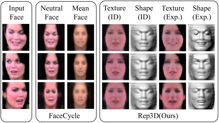
Fig. 3: Comparison of disentangled representations. Our method have a more detailed and fidelity representation than the SOTA method FaceCycle [11].

3.5 Ablation Study

Tab. 2 presents an ablation study for 3D-aware autoencoders and latent disentangling methods for facial expression classification on RAF-DB and face verification on LFW. Factors like light and pose are critical for the convergence of 3D-aware autoencoders, and their absence results in a significant drop in performance. Furthermore, the removal of the Representation Diffusion Model (RDM) leads to a notable 6.62% decrease in RAF-DB and 4.17% in LFW.

To underscore the significance of RDM in latent disentangling, we explore an alternative approach using a ResNet encoder to predict the identity latent from the face image, referred to as the encoder-based method. However, the model encounters difficulties due to the noisy dataset, where the identity is hard to predict from images. In contrast, the latent disentangling is more useful, and the performance enhancement of RDM is more substantial, with a 3% advantage on RAF-DB. Additionally, we also conduct experiments regarding RDM for different 3D factors. Disentangling facial shape is more important than texture for facial expression and otherwise for face verification.

4 Conclusion

This paper presents a novel unsupervised disentangling framework for facial expression and identity representations. We suggest that the disentangling should be performed in latent space and propose a novel 3D-aware latent diffusion model. Experimental results demonstrate that our approach can achieve SOTA performance.

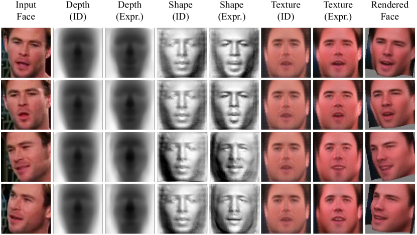
Fig. 4: Visualization of intermediate results. The depth images describe the raw depth map, while the shape images are obtained by shading the depth maps with predicted lights for better visualization.

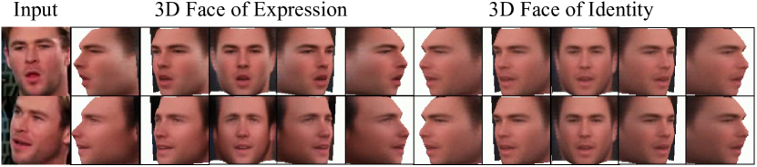
Fig. 5: Visualization of generated facial identity. We show the reconstructed 3D face of 2 frames in the input video sequence. The facial identity is disentangled from expressions.

5 Supplementary Materials

5.1 More Visualization

Fig. 4 displays visualizations of intermediate results of the model. We present extracted facial textures and shapes, including the original face, the face of the identity, and the rendered face. Facial shapes can be represented using depth maps from canonical views (columns two and three), but these do not capture fine details well. Therefore, we utilize predicted lighting to visualize the facial shape (columns four and five). Fig. 5 further illustrates the comparison between our generated facial identities and expressions in 3D. Our approach disentangles facial identity and obtains the same facial identity representation for different faces.

To further show the advantage of our model in pose disentangling, we show the results of face frontalization compared with other methods on the CelebA dataset in Fig. 6. Our method can synthesize a frontal image of a human face with the extracted facial texture and depth by setting the pose in the canonical view. We compare the cosine distance of Arcface [26] embedding between the frontalized face with the original face. The generated faces of [11] are blurry and have artifacts. Our model can make light and pose disentangled from the environment and restore the occluded face’s color information, achieving lower Arcface distances than [11].

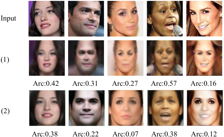
Fig. 6: Face frontalization results. (1) is the output of the state-of-the-art method FaceCycle[11]. (2) Our model can restore the complete front face with lower Arcface distance.

5.2 More Experiments

For facial expression recognition, we further evaluate the confusion matrix of our predictions on AffectNet. In AffectNet, the classes with the lowest accuracy are ’disgust’ (26%) and ’contempt’ (25%). We hypothesize that the classification performance is impacted by the dataset’s imbalance. Notably, the ’disgust’ and ’contempt’ classes comprise the smallest proportion of the dataset, each representing only 5% of the samples in the ’neutral’ category. We propose that balancing the dataset might improve classification accuracy.

For face verification, we also follow the LFW [24] protocol to incorporate more metrics for performance assessment, such as Equal Error Rate (EEr) and False Rejection Rate (FRR) at given False Acceptance Rate (FAR) values in Tab. 3 and Detection Error Tradeoff (DET) curves in Fig. 8. Our comparisons with FaceCycle reveal that our model maintains superiority over the current state-of-the-art (SOTA) method.

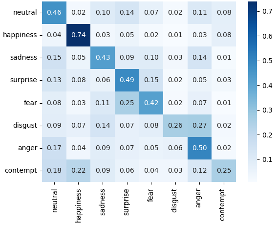
Fig. 7: Confusion matrix analysis on AffectNet dataset. We show actual classes in y-axis and predicted classes in x-axis.

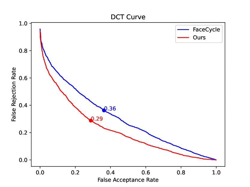
Fig. 8: DCT curve analysis on LFW dataset. We show the equal error rate (EER) point on the curve. Our model demonstrates lower error rates on face verification.

	EEr	FRR@1%	FRR@5%	FRR@20%
FaceCycle	0.3626	0.8626	0.7259	0.5206
Ours	0.2879	0.8090	0.6363	0.3853

Table 3: Evaluation of Equal Error Rate (EEr) and False Rejection Rate (FRR) at given False Acceptance Rate (FAR).

5.3 Network Details

For the architecture of the encoders, we partition them into feature encoders and numerical encoders by structure. The feature encoder refers to the facial texture encoder and the facial shape encoder. They work with the decoder to encode the two-dimensional features of the face. Figure 9 shows the detailed structure. The two encoders have the same architecture, and what they produce is a 256-dimensional vector. We use a fully convolutional architecture to reduce the influence of our features on the position of the pose. Our decoder uses stacked convolutional layers, transposed convolutional layers, and group normalization layers. Figure 11 shows the detailed structure. The network uses a 256-dimensional vector as input. The facial texture decoder produces a 3-channel two-dimensional image output, while the facial shape decoder produces 1 channel. The final texture map and depth map will be scaled by Tanh to the range of -1 to 1.

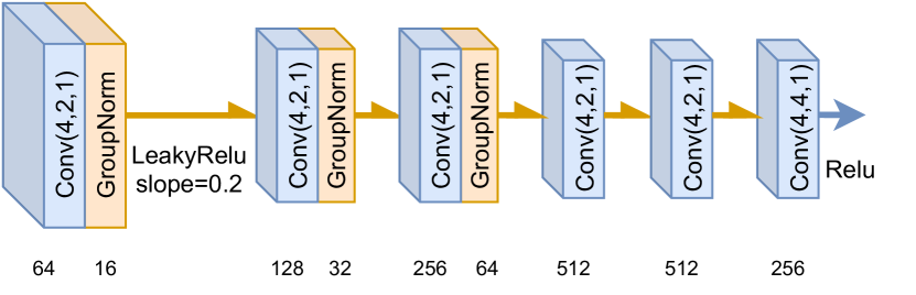
Fig. 9: Feature Encoder Architecture. $Conv(a,b,c)$ indicates that the kernel size of the convolutional layer is $a$, the stride is $b$, and the padding is $c$. The number below the convolutional layer indicates the number of convolution kernels. The number below the group normalization layer indicates the number of groups. The yellow arrow indicates Leaky Relu, with a slope of 0.2. And the blue arrow is Relu.

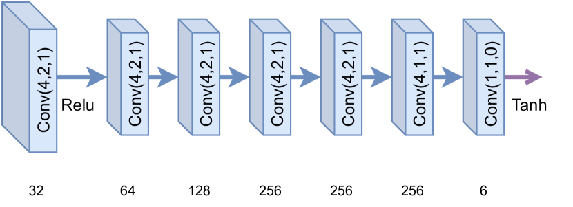
Fig. 10: Numerical Encoder Architecture. It is a fully convolutional network. $Conv(a,b,c)$ indicates that the kernel size of the convolutional layer is $a$, the stride is $b$, and the padding is $c$. The number below the module indicates the number of convolution kernels. The blue arrow is Relu. And the purple arrow is Tanh.

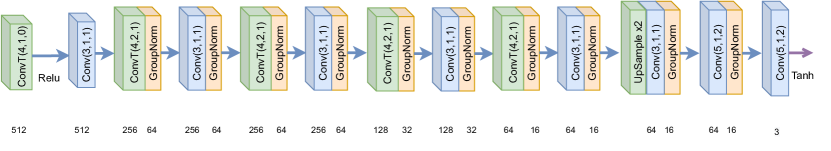
Fig. 11: Decoder Architecture. $Conv(a,b,c)$/$ConvT(a,b,c)$ indicates that the kernel size of the convolutional layer/transposed convolutional layer is $a$, the stride is $b$, and the padding is $c$. The number below the module indicates the number of convolution kernels. And The number below the group normalization layer indicates the number of groups.

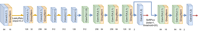
Fig. 12: Confidence Map decoder Architecture. The yellow arrow indicates Leaky Relu, with a slope of 0.2. And the blue arrow is Relu. The red arrow is a SoftPlus operator with beta=1 and threshold=20. The shorter path is for the feature level loss and the longer path is for the photometric loss.

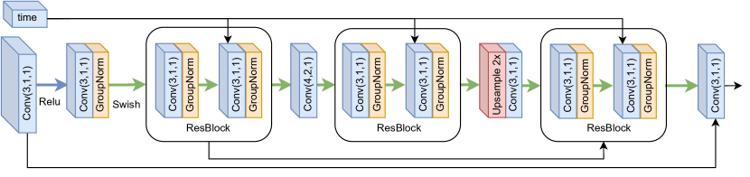
Fig. 13: Denoising U-Net Architecture. $Conv(a,b,c)$ indicates that the kernel size of the convolutional layer is $a$, the stride is $b$, and the padding is $c$. The number of convolution kernels are set to 512, except for the last one which is 256. The blue arrow is Relu while the green arrow is Swish Gate. We use sinusoidal timestep embeddings defined in [27]. We omit the skip connections in the ResBlocks[28] for a clear view.

The numerical encoder refers to the light and head pose encoder. Figure 10 shows the detailed structure. They generate corresponding values separately to set the rendering condition. These two encoders have the same structure, except that the output vector dimensions are slightly different. The head pose encoder has 6 dimensions, which are the translation vector of x, y, and z and the rotation angle of yaw, roll, and pitch. The light encoder has 4 dimensions: ambient light parameters, diffuse reflection parameters, and two light directions $(x,y)$. We will first use Tanh to scale the final outputs to $[-1,1]$, and then map them to the corresponding space.

Following [16], we use a similar structure as the depth encoders and decoders to generate the confidence map for the self-calibration of the loss function. Figure 13 shows the network structure. We use the relu3_3 feature extracted by a pretrained VGG16[29] network for feature-level loss. The VGG networks can also be replaced with self-supervised discriminators as demonstrated by [16].

For the architecture of the denoising U-Net[30], we use one downsample block, one middle block, and one upsample block, with two ResNet[28] layers in each block. Figure 13 shows the network structure. The input 256-dimensional noise is concatenated with the facial texture latent or the facial shape latent. Therefore, the input size is 512. Then we expand the 512 dimensional vector to a 512$\times$3$\times$3 feature by padding zeros. The output size is 256 dimensional, the same as the input noise. The facial texture latent diffusion model and facial shape latent diffusion model are learned separately.

5.4 Loss Function

In the first stage, our reconstruction loss is composed of a pixel-level loss $L_{p}(\hat{I},I)$, a feature-level loss $L_{f}(\hat{I},I)$, which measure the photometric discrepancy in pixel level, and feature level separately, which is also used by many works[31, 32, 16].

$$L_{p}(\hat{I},I) =L_{\mathit{conf}}(\hat{I},I,\sigma_{p})$$ (5)

$$L_{f}(\hat{I},I) =L_{\mathit{conf}}(\mathit{conv}(\hat{I}),\mathit{conv}(I),\sigma_{f}),$$ (6)

where $I$ represents the input image and $\hat{I}$ is the reconstructed image. The reconstruction losses are constrained with estimated confidence maps $\sigma$ to make the model self-calibrate [33].

$$L_{\mathit{conf}}(\hat{I},I,\sigma)=-\frac{1}{|\Omega|}\sum_{u,v\in\Omega}\ln\frac{1}{\sqrt{2}\sigma_{u,v}}\exp-\frac{\sqrt{2}(\hat{I}-I)_{u,v}}{\sigma_{u,v}}$$ (7)

where $L$ is the reconstruction loss, and $u,v$ is the pixel on the rendered face mask $\Omega$. We separately predict the confidence map $\sigma_{p}$ and $\sigma_{f}$ from the image with an encoder-decoder structure for the pixel-level and feature-level loss. A pretrained VGG-19[29] is leveraged for the low-level feature extraction network $\mathit{conv}$.

The reconstruction loss $L(\hat{I},I)$ can be expressed as a linear combination of the pixel-level loss, and the feature-level loss.

$$L(\hat{I},I)= L_{p}(\hat{I},I)+\lambda_{f}L_{f}(\hat{I},I)$$ (8)

$$+\lambda_{flip}(L_{p}(\hat{I}^{\prime},I)+\lambda_{f}L_{f}(\hat{I}^{\prime},I))$$ (9)

where $\lambda_{f}$ are the weight for the feature-level. Moreover, we also calculate the reconstructed image $\hat{I}^{\prime}$ of the horizontally flipped shape and texture code for the symmetric loss function. $\lambda_{flip}$ is the weight for flipped reconstruction loss. The hyperparameters in the loss function are set as follows: $\lambda_{f}=1,\lambda_{flip}=0.5$.

For the second stage, we optimize the denoising U-Net $\mathcal{E}_{r}$ with Eq. 4. Following [34, 19], we use the SNR weighting strategy, which uses different weights for different steps. For given target latent $Z_{0}$ and our predictions $\hat{Z}_{0}$, the denoising loss can be expressed as:

$$L(\hat{Z}_{0},Z_{0})=E_{Z_{0},\epsilon,t}\left[w_{t}\left\|Z_{0}-\mathcal{E}_{r}\left(Z_{t},t,Z_{exp}\right)\right\|^{2}\right]$$ (10)

where $w_{t}$ is the SNR weight depended on step $t$, which can be expressed as $w_{t}=\frac{\alpha_{t}^{2}}{1-\alpha_{t}^{2}}$. $\alpha_{t}$ is the noise schedule in [27]. Like the latent diffusion models[19], the encoders and decoders are frozen when training the denoising U-Net.

5.5 Rendering Pipeline

In order to render a face image, we need to know: facial shape, facial texture, lighting, and head pose. The facial shape is represented as a two-dimensional single-channel matrix, which represents the depth map of the face. We define a grid, the size of the grid is the same as the image, which is 64 $\times$ 64. Their x-axis and y-axis coordinates are scaled to between -1 and 1, and then the z-axis coordinates come from the depth map. In this way, we get a three-dimensional model of the human face and the normal of every point for later calculation.The facial texture is represented as a 3-channel 2D matrix in the renderer. It indicates the diffuse reflectance of each face grid point of RGB rays.

Lighting includes ambient light intensity, diffuse reflection intensity and light direction x, y. We are modeling directional light, so only two variables are needed to describe the direction of light. According to the illumination equation [35], we already know the ambient light intensity $k_{\text{a}}$ , diffuse reflection intensity $k_{\text{d}}$, light direction vector ${\mathbf{L}}_{m}$, and the surface normal vector ${\mathbf{N}_{p}}$ of each point, and the diffuse reflection coefficient $k_{\text{d},\text{p}}$. Our model ignores the specular reflection of the human face. In most cases, the specular reflection coefficient of the human face is small enough to omit.

The head pose is actually described as the camera parameters. The movement of the head relative to the camera and the change of the camera’s shooting angle are mutual processes. Thus, we only need to control the camera’s shooting displacement vector under x, y, z, and the rotation angle yaw, roll, pitch. We can apply these parameters to the camera imaging equation as below. The displacement vector is $\mathbf{t}$ and the rotation vector is $\mathbf{R}$. And we define the camera matrix $\mathbf{K}$ as $diag(f,f,1)$, where $f$ is the focal length. The focal length can be calculated as $\frac{1}{f}=2\tan\frac{\theta_{FOV}}{2}$, where $\theta_{FOV}$ is set as 10 degrees.

In short, we first build a three-dimensional skeleton of the face shape, and then map the face material to the three-dimensional skeleton. Then we use the light information to determine the color of the face. Finally, we use the camera formula to get the image we took at a specific angle.

References

- [1] Michael E Hasselmo, Edmund T Rolls, and Gordon C Baylis, “The role of expression and identity in the face-selective responses of neurons in the temporal visual cortex of the monkey,” Behavioural brain research, vol. 32, no. 3, pp. 203–218, 1989.
- [2] Qiong Cao, Li Shen, Weidi Xie, Omkar M. Parkhi, and Andrew Zisserman, “Vggface2: A dataset for recognising faces across pose and age,” in FG, 2018, pp. 67–74.
- [3] Kai Wang, Xiaojiang Peng, Jianfei Yang, Debin Meng, and Yu Qiao, “Region attention networks for pose and occlusion robust facial expression recognition,” TIP, vol. 29, pp. 4057–4069, 2020.
- [4] Jiabei Zeng, Shiguang Shan, and Xilin Chen, “Facial expression recognition with inconsistently annotated datasets,” in ECCV, 2018, pp. 222–237.
- [5] Xiao Gu, Yao Guo, Zeju Li, Jianing Qiu, Qi Dou, Yuxuan Liu, Benny Lo, and Guang-Zhong Yang, “Tackling long-tailed category distribution under domain shifts,” in ECCV. Springer, 2022, pp. 727–743.
- [6] Dimitrios Kollias, “Abaw: Valence-arousal estimation, expression recognition, action unit detection & multi-task learning challenges,” in CVPR, 2022, pp. 2328–2336.
- [7] Ting Chen, Simon Kornblith, Mohammad Norouzi, and Geoffrey Hinton, “A simple framework for contrastive learning of visual representations,” in International conference on machine learning. PMLR, 2020, pp. 1597–1607.
- [8] Kaiming He, Xinlei Chen, Saining Xie, Yanghao Li, Piotr Dollár, and Ross Girshick, “Masked autoencoders are scalable vision learners,” in CVPR, 2022, pp. 16000–16009.
- [9] Yong Li, Jiabei Zeng, Shiguang Shan, and Xilin Chen, “Self-supervised representation learning from videos for facial action unit detection,” in CVPR, 2019, pp. 10916–10925.
- [10] Liupei Lu, Leili Tavabi, and Mohammad Soleymani, “Self-supervised learning for facial action unit recognition through temporal consistency,” in BMVC, 2020.
- [11] Jia-Ren Chang, Yong-Sheng Chen, and Wei-Chen Chiu, “Learning facial representations from the cycle-consistency of face,” in ICCV, 2021, pp. 9660–9669.
- [12] Yuxuan Shu, Xiao Gu, Guangyao Yang, and Benny P. L. Lo, “Revisiting self-supervised contrastive learning for facial expression recognition,” in BMVC, 2022.
- [13] Shan Li, Weihong Deng, and JunPing Du, “Reliable crowdsourcing and deep locality-preserving learning for expression recognition in the wild,” in CVPR, 2017, pp. 2584–2593.
- [14] Ali Mollahosseini, Behzad Hasani, and Mohammad H. Mahoor, “Affectnet: A database for facial expression, valence, and arousal computing in the wild,” IEEE Transactions on Affective Computing, vol. 10, no. 1, pp. 18–31, 2019.
- [15] Ziwei Liu, Ping Luo, Xiaogang Wang, and Xiaoou Tang, “Deep learning face attributes in the wild,” in ICCV, 2015, pp. 3730–3738.
- [16] Shangzhe Wu, Christian Rupprecht, and Andrea Vedaldi, “Unsupervised learning of probably symmetric deformable 3d objects from images in the wild,” TPAMI, pp. 1–1, 2021.
- [17] Volker Blanz and Thomas Vetter, “A morphable model for the synthesis of 3d faces,” in SIGGRAPH, 1999, p. 187–194.
- [18] Arsha Nagrani, Joon Son Chung, and Andrew Zisserman, “VoxCeleb: A Large-Scale Speaker Identification Dataset,” in Proc. Interspeech 2017, 2017, pp. 2616–2620.
- [19] Robin Rombach, A. Blattmann, Dominik Lorenz, Patrick Esser, and Björn Ommer, “High-resolution image synthesis with latent diffusion models,” CVPR, pp. 10674–10685, 2021.
- [20] Jonathan Ho, Ajay Jain, and Pieter Abbeel, “Denoising diffusion probabilistic models,” in NeurIPS, 2020, vol. 33, pp. 6840–6851.
- [21] Florian Schroff, Dmitry Kalenichenko, and James Philbin, “Facenet: A unified embedding for face recognition and clustering,” pp. 815–823, 2015.
- [22] Dimitrios Kollias, Irene Kotsia, Elnar Hajiyev, and Stefanos Zafeiriou, “Analysing affective behavior in the second abaw2 competition,” 2021.
- [23] Hangyu Li, Nannan Wang, Xi Yang, Xiaoyu Wang, and Xinbo Gao, “Towards semi-supervised deep facial expression recognition with an adaptive confidence margin,” in CVPR, 2022, pp. 4166–4175.
- [24] Gary B. Huang Erik Learned-Miller, “Labeled faces in the wild: Updates and new reporting procedures,” Tech. Rep. UM-CS-2014-003, University of Massachusetts, Amherst, May 2014.
- [25] Weihong Deng, Jiani Hu, Nanhai Zhang, Binghui Chen, and Jun Guo, “Fine-grained face verification: Fglfw database, baselines, and human-dcmn partnership,” Pattern Recognition, vol. 66, pp. 63–73, 2017.
- [26] Jiankang Deng, Jia Guo, Niannan Xue, and Stefanos Zafeiriou, “Arcface: Additive angular margin loss for deep face recognition. in 2019 ieee,” in CVPR, 2018, pp. 4685–4694.
- [27] Jonathan Ho, Ajay Jain, and P. Abbeel, “Denoising diffusion probabilistic models,” arXiv, vol. abs/2006.11239, 2020.
- [28] Kaiming He, Xiangyu Zhang, Shaoqing Ren, and Jian Sun, “Deep residual learning for image recognition,” pp. 770–778, 2016.
- [29] Karen Simonyan and Andrew Zisserman, “Very deep convolutional networks for large-scale image recognition,” 2015.
- [30] Olaf Ronneberger, Philipp Fischer, and Thomas Brox, “U-net: Convolutional networks for biomedical image segmentation,” arXiv, vol. abs/1505.04597, 2015.
- [31] Yu Deng, Jiaolong Yang, Sicheng Xu, Dong Chen, Yunde Jia, and Xin Tong, “Accurate 3d face reconstruction with weakly-supervised learning: From single image to image set,” in 2019 IEEE/CVF Conference on Computer Vision and Pattern Recognition Workshops (CVPRW), 2019, pp. 285–295.
- [32] Yao Feng, Haiwen Feng, Michael J. Black, and Timo Bolkart, “Learning an animatable detailed 3d face model from in-the-wild images,” ACM Trans. Graph., vol. 40, no. 4, jul 2021.
- [33] Alex Kendall and Yarin Gal, “What uncertainties do we need in bayesian deep learning for computer vision?,” in NeurIPS, Isabelle Guyon, Ulrike von Luxburg, Samy Bengio, Hanna M. Wallach, Rob Fergus, S. V. N. Vishwanathan, and Roman Garnett, Eds., 2017, pp. 5574–5584.
- [34] Jonathan Ho, Tim Salimans, Alexey Gritsenko, William Chan, Mohammad Norouzi, and David J. Fleet, “Video diffusion models,” arXiv, vol. abs/2204.03458, 2022.
- [35] Bui Tuong Phong, “Illumination for computer generated pictures,” Commun. ACM, vol. 18, no. 6, pp. 311–317, jun 1975.