A Hybrid Quantum-assisted Column Generation Algorithm for the Fleet Conversion Problem

Abstract.

The problem of Fleet Conversion aims to reduce the carbon emissions and cost of operating a fleet of vehicles for a given set of tours. It can be modelled as a column generation scheme with the Maximum Weighted Independent Set(MWIS) problem as the slave. Quantum variational algorithms have gained significant interest in the past several years. Recently, a method to represent Quadratic Unconstrained Binary Optimization(QUBO) problems using logarithmically fewer qubits was proposed. Here we use this method to solve the MWIS Slaves and demonstrate how quantum and classical solvers can be used together to approach an industrial-sized use-case (up to 64 tours).

1. Introduction

Fleet conversion is the process of transitioning a fleet of vehicles to more sustainable and environmentally friendly alternatives. With the growing recognition of the detrimental effects of traditional fossil fuel powered vehicles on the environment and the need to mitigate climate change, businesses and organizations are increasingly looking for ways to reduce their carbon footprint and operate more efficiently. The transportation sector is one of the largest contributors to greenhouse gas emissions, primarily due to their reliance on fossil fuels. By transitioning fleets to electric or hybrid vehicles, companies can significantly reduce their carbon emissions. Beyond the environmental benefits, fleet conversion also offers compelling cost-saving opportunities for businesses.

In the fleet conversion problem, a certain number of tours need to be carried out between several locations. In order to carry out these tours we have at our disposal several vehicles of different models. Each vehicle model has an associated cost. On top of the capital expenditure corresponding to the purchase of one vehicle of one model, this cost may also capture the environmental cost – e.g. the carbon footprint; the cost of operation – e.g. energy usage, or both. The objective is to minimize the total cost of carrying out all the tours including capital and operational expenditures. Therefore, fleet conversion goes beyond simply choosing the best possible vehicles and also incorporates sharing the same vehicles for multiple tours when possible, thereby reducing the cost.

Quantum computing (Nielsen and Chuang, 2011; Preskill, 2021, 2018) is a potentially disruptive field that could have applications in several domains including financial modelling (Orús et al., 2019; Herman et al., 2022), cryptography (Scarani et al., 2009; Mehic et al., 2020), chemistry (Martin et al., 2022; Haidar et al., 2023) and optimization. Within the scope of optimization applications, there has been a growing interest in quantum variational algorithms (Bittel and Kliesch, 2021; Cerezo et al., 2021; Callison and Chancellor, 2022; Peruzzo et al., 2014; Nakanishi et al., 2020; Moll et al., 2018; Lubasch et al., 2020; Stokes et al., 2020). Among them, the Quantum Approximate Optimization Algorithm (QAOA) has been heavily researched (Farhi et al., 2014; Fuchs et al., 2021; Herrman et al., 2021; Larkin et al., 2022; Zhou et al., 2020; Hadfield et al., 2019). A well known issue with QAOA is that it does not scale well with problem size limiting its applications to toy problems . Recently, an algorithm to treat Quadratic Unconstrained Binary Optimization (QUBO) (Glover et al., 2019; Date et al., 2021; Calude et al., 2017; Papalitsas et al., 2019) problem using logarithmically fewer qubits has been demonstrated(Rančić, 2023; Chatterjee et al., 2023). In this paper, we use column generation (Desaulniers et al., 2006; Barnhart et al., 1998; Wilhelm, 2001; Demiriz et al., 2002; Mehrotra and Trick, 1996) to describe our problem as a master problem and several sub-problems henceforth referred to as slaves. The slave problem in our case is the Maximum Weighted Independent Set (MWIS) problem which can be represented as a QUBO problem. We propose an algorithm that handles the master problem using a commercial linear program solver Gurobi and the slave problems using a quantum solver based on (Chatterjee et al., 2023). In our experiments, we solve instances up to a size of 64 tours using only 7 qubits to represent the MWIS Slaves. This shows that the method is compatible with the quantum computers of the NISQ era.

The paper is structured as follows. In section 2.1 the fleet conversion problem is defined. In section 2.2 the problem is stated in the form of a graph problem followed by section 2.3 where the column generation algorithm is described. In section 2.4 and 2.5, we describe the quantum model to solve the sub-problems and how we can use the quantum solver and classical solver together to develop a quantum-assisted algorithm. Finally, we present the experimental results in section 3.

2. Problem Statement and Methods

In this section, we present the Fleet Conversion Problem as well as its formulation as a weighted graph coloring problem. We then reformulate the problem using the definition of independent sets and build a column generation approach to solve it. The column generation approach uses sub-problems that compute max-weighted independent sets, further brought together iteratively to build a global graph coloring solution. We then demonstrate how a quantum algorithm can be crafted to solve these sub-problems and integrate the column generation procedure.

2.1. Statement

Let $L$ be a set of locations, $K$ a set of tours, $V$ a set of available vehicle models, and $C$ a set of physical vehicles, henceforth referred to as color.

Notations.

For any physical vehicle $c$ of a certain model $v$, let us write $v(c):=v$. Tours are carried out from one location to another. Let $w^{k}_{v}$ be the cost to assign a vehicle model $v$ to any tour $k$. Assigning a model $v$ to a tour $k$ means that the tour $k$ has to be carried out by a physical vehicle (color) from model $v$. To do so, some color $c$ such that $v(c)=v$ has to be assigned to tour $k$. The cost $w_{v}^{k}$ captures the operational expenditures incurred by performing tour $k$ with a vehicle model $v$. Since every color belongs a specific vehicle model, let the cost to assign the physical vehicle (color) $c$ to any tour $k$ be $\Gamma^{k}_{c}\coloneqq w^{k}_{v}$ when $v=v(c)$. We also define a cost $\gamma_{v(c)}>0$ for using a color $c$ at least once. Clearly, $\gamma_{v}$ represents the cost of purchase of one physical vehicle of model $v$ and we reasonably assume this cost is independent of the color (all vehicles of the same model are equivalent). Thus, without risk of confusion, we define $\gamma_{c}\coloneqq\gamma_{v(c)}$.

Each tour $k\in K$ is described by the tuple $(t_{d}^{k},t_{a}^{k},l_{d}^{k},l_{a}^{k},A^{k})$, corresponding respectively to the departure time, arrival time, departure location and arrival location, and a set of authorized vehicle models of the tour. The time to travel from location $i$ to location $j$ ($TT_{ij}$) can be computed using the distance matrix of the locations. This matrix is used to derive the time needed to relocate any physical vehicle from the arrival location of a tour to the departure location of another tour in case these tours are meant to be assigned to the same color.

Incompatibilities.

In the Fleet Conversion Problem, we have two types of incompatibilities:

• tour-color incompatibilities: a tour $k$ cannot be assigned to a color from a certain model $v$. In practice, this incompatibility can model constraints in urban mobility such as the forbidden penetration of internal combustion engines into low emission zones or simply drivers’ personal preferences (manual vs automatic, plug-in hybrid vs electric, etc). Let $A^{k}$ be the set of authorized colors for tour $k$. Specifically, a color $c$ can be assigned to tour $k\in K$ only if $v(c)$ is in the set of allowed models $A^{k}$ for that tour.

• tour-tour incompatibilities: two different tours cannot share the same color (physical vehicle) because they occur at the same time, or because their departure and/or arrival locations make it impossible to transition in an acceptable time without perturbing the global schedule. Let $\mathcal{I}\subset\binom{{K}}{2}$ be the set of unordered couples with a tour-tour incompatibility.

First formulation.

The aim of the Fleet Conversion Problem is to minimize the overall cost $\sum_{c}\gamma_{c}y_{c}+\sum_{k,c}\Gamma^{k}_{c}x_{c}^{k}$, where

(1) $$x^{k}_{c}=\left\{\begin{matrix}1&\mbox{if color $c$ is assigned to tour $k$}\\ 0&\mbox{otherwise,}\end{matrix}\right.$$

and

(2) $$y_{c}=\left\{\begin{matrix}1&\mbox{if color $c$ is purchased}\\ 0&\mbox{otherwise.}\end{matrix}\right.$$

This can be achieved by preferring colors $c$ with low values of $\gamma_{c}$ and also by assigning multiple compatible tours to a single color while choosing the minimal values of $\Gamma_{c}^{k}$ if possible. This is to be done in such a way that all tours within $K$ are assigned to a compatible color.

Therefore, the Fleet Conversion Problem can be expressed as the following optimization problem:

(3) $$\min \sum_{c\in C}\gamma_{c}y_{c}+\sum_{k\in K,c\in C}\Gamma^{k}_{c}x_{c}^{k}$$

(4) s.t. $$\sum_{c}x^{k}_{c}\geq 1 (\forall k\in K)$$

(5) $$x^{k}_{c}\leq y_{c} (\forall c\in C)(\forall k\in K)$$

(6) $$x^{k}_{c}+x^{k^{\prime}}_{c}\leq 1 (\forall\{k,k^{\prime}\}\in\mathcal{I})(\forall c\in C)$$

(7) $$x^{k}_{c}=0 (\forall k\in K)(\forall c\in C)(v(c)\notin A^{k})$$

(8) $$y_{c},x_{c}^{k}\in\{0,1\}.$$

Equation (4) states that a tour $k$ has to be assigned to at least one color, whereas Equation (5) forbids the assignment of tours to a color unless the color is purchased. Equation (6) forbids incompatible tours to share the same color and Equation (7) avoids tour-color incompatibilities.

Problem (3)–(8) is thus a Mixed Integer Linear Program (MILP) that can be solved with for instance a commercial solver. However, as it is notoriously NP-complete as from $|C|\geq 3$, solver time performance will worsen quickly with problem size. For this reason, we reformulate Problem (3)–(8) and design an algorithm that will scale better.

2.2. Formal description as a Graph Problem

Let $G=(K,E)$ be a graph where the nodes of the graph are the tours and the edges $(k,k^{\prime})\in E$ of the graph denote the incompatibility of the tours $k$ and $k^{\prime}$. With the notations of the last paragraph, this means that we let $E:=\mathcal{I}$. Two tours $i$ and $j$ are compatible if their time-windows do not overlap and we have enough time to travel from the arrival location of tour $i$ to the departure location of tour $j$, without loss of generality if tour $i$ occurs before tour $j$. Formally, we define $E=\{(i,j)|\forall i,j\in K,t_{a}^{i}+TT_{ij}>t_{d}^{j}\}$. For every tour $k$, we have a list of allowed models $A^{k}$.

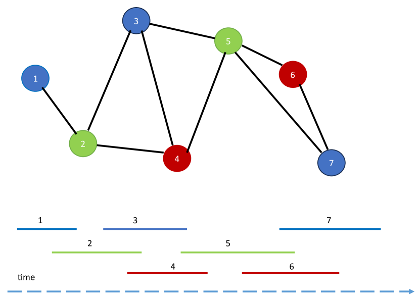
Figure 1. Incompatibility Graph generated from the time windows of tours. The lines represent the time windows of 7 tours. Colors blue, red and green are used to assign vehicles to tours taking into account their incompatibility.

Figure 1 illustrates how an incompatibility graph can be constructed using time-windows of several tours, along with a possible coloring of the graph. For example, since the tour 3 overlaps with tours 2, 4 and 5, the node 3 has edges with node 2, 4 and 5.

Definition 2.1 (Independent set).

An independent set in $G=(K,E)$ is a subset $I\subseteq K$, such that for any two vertices $k,k^{\prime}\in I$, $(k,k^{\prime})\notin E$. In other words, an independent set of our graph is a subset of tours that are all compatible with each other to share colors.

With the definition of an independent set, the following fact is straightforward.

Fact 1.

Let $(x,y)$ be any solution of Problem (3)–(8). Then, for all $c\in C$ such that $y_{c}=1$, $\{k|x_{c}^{k}=1\}$ forms an independent set of $G$.

An independent set $I$ can be derived into an allocation $(a_{I},c_{I})$, where $c_{I}\in C$ is a color and $a_{I}$ is the indicator vector of set $I$: $a^{k}_{I}=1$, if $k\in I$, and $0$ otherwise. For any independent set $I$ and color $c$, let $\Gamma_{I,c}:=\gamma_{c}+\sum_{k\in I}\Gamma^{k}_{c}$ denote the cost of allocation $(a_{I},c)$. Here, we consider only feasible allocations, specifically respecting tour-color compatibility. We can therefore define the set of feasible allocations $\Lambda$ formally as :

(9) $$\Lambda=\{(a_{I},c_{I})|I\mbox{ independent set of }G|\mbox{ s.t. }\forall k\in K,a^{k}_{I}=1\Rightarrow v(c_{I})\in A^{k}\}.$$

For lighter notations, we refer to the element $(a_{I},c_{I})\in\Lambda$ only as $I\in\Lambda$, keeping in mind that the independent set $I$, considered as an allocation, comes with a color $c_{I}$. In particular, we keep in mind that if $c\neq c^{\prime}$, and even if $v(c)=v(c^{\prime})$, $(a_{I},c)$ and $(a_{I},c^{\prime})$ are two different allocations. Formally, let $\Gamma_{I}\coloneqq\Gamma_{I,c_{I}}$.

The problem can then be equivalently formulated as:

(10) $$\min \sum_{I\in\Lambda}\Gamma_{I}x_{I}$$

(11) s.t. $$\sum_{I\in\Lambda}a_{I}^{k}x_{I}\geq 1 (\forall k\in K)$$

(12) $$x_{I}=\begin{cases}1,\text{ if independent set }I\text{ chosen }\\ 0,\text{ otherwise}\end{cases}$$

Note that constraint (11) is equivalent to the constraint (4). Also, beware that the variables defined in equation (12) and equation (1) are not the same.

With the above reformulation, the problem looks considerably smaller. We have indeed only one constraint per tour. However, we need to generate the set $\Lambda$ in order to solve this problem. The set $\Lambda$ contains all the feasible independent sets of the graph, that is, independent set of the graph coupled with colors that are compatible with all nodes therein. Remember that if $I$ is a non-empty independent set of $G$ and $c\neq c^{\prime}$ are two different colors, then $(I,c)$ and $(I,c^{\prime})$ are two distinct elements of $\Lambda$ as they describe two different conversion solutions. We thus have a very large number of variables $x_{I}$. Nevertheless, it is clear that only a small number of those variables should be non-zero at optimum. Indeed, at worst (in terms of number of independent sets activated), no sharing of color is possible and each tour has a dedicated vehicle, which corresponds to $|K|$ variables $x_{I}$ activated. This is why an interesting approach here is column generation, where independent sets are generated dynamically while the solution converges to an optimum.

2.3. The Column Generation Algorithm

In this paragraph, we design the column generation procedure to solve our problem. First, we derive an extension of the problem that makes it always feasible. To do so, we permit the algorithm to reject tours from the solution. Second, we relax all integrity constraints and actually solve the LP-relaxation of our problem. Once an LP-optimal solution is found by the column generation, one can summon any type of rounding algorithm to build (if needed) an integer-feasible solution from the relaxed solution. For instance, see (Bertsimas et al., 1999). We focus this work on the problem of finding the optimal LP-feasible solution for our problem.

Problem extension

For all $k\in K$, let $r_{k}$ be a binary variable that states whether tour $k$ is rejected from the solution or not:

(13) $$r_{k}=\left\{\begin{matrix}1&\mbox{if }k\mbox{ is rejected}\\ 0&\mbox{otherwise.}\end{matrix}\right.$$

Let $R$ be a sufficiently large real number. We now consider the new optimization problem:

(MP) $$\min \sum_{I\in\Lambda}\Gamma_{I}x_{I}+R\sum_{k\in K}r_{k}$$

(MP-1) s.t. $$\sum_{I\in\Lambda}a_{I}^{k}x_{I}+r_{k}\geq 1 (\forall k\in K)$$

(MP-2) $$x_{I},r_{k}\geq 0 (\forall I\in\Lambda)(\forall k\in K)$$

When the binary constraints are enforced on $x_{I}$ and $r_{k}$, and if $R$ is sufficiently large, it is clear that Problems (MP) and (10)–(11) are equivalent. The dual program (Balinski and Tucker, 1969) of (MP) reads :

(D) $$\max \sum_{k\in K}\mu_{k}$$

(D-1) s.t. $$\sum_{k\in K}a^{k}_{I}\mu_{k}\leq\Gamma_{I} (\forall I\in\Lambda)$$

(D-2) $$\mu_{k}\geq 0 (\forall k\in K)$$

Restriction and generation

Let $\Lambda^{\prime}\subset\Lambda$ be an arbitrary subset of allocations. One can form the primal dual pair of problems:

(RMP) $$\min \sum_{I\in\Lambda^{\prime}}\Gamma_{I}x_{I}+R\sum_{k\in K}r_{k}$$

(RMP-1) s.t. $$\sum_{I\in\Lambda^{\prime}}a_{I}^{k}x_{I}+r_{k}\geq 1 (\forall k\in K)$$

(RMP-2) $$x_{I},r_{k}\geq 0 (\forall I\in\Lambda^{\prime})(\forall k\in K)$$

(RD) $$\max \sum_{k\in K}\mu_{k}$$

(RD-1) s.t. $$\sum_{k\in K}a^{k}_{I}\mu_{k}\leq\Gamma_{I} (\forall I\in\Lambda^{\prime})$$

(RD-2) $$\mu_{k}\geq 0 (\forall k\in K)$$

Let $F$ (resp. $F^{\prime}$) denote the feasible set of (MP) (resp. (RMP)) and $G$ (resp. $G^{\prime}$) be the feasible set of (D) (resp. (RD)). It is clear that $F^{\prime}\subset F$ and $G\subset G^{\prime}$. Furthermore, for any $\Lambda^{\prime}\subset\Lambda$, (RMP) is linear, feasible and bounded. Therefore, strong-duality applies (Balinski and Tucker, 1969)(Gale et al., 1951). This means that (RMP) and (RD) are both feasible and a primal-dual pair of solutions $(x^{\prime},\mu^{\prime})$ exists, where $x^{\prime}$ solves (RMP), $\mu^{\prime}$ solves (RD). Furthermore, it means we have the equality:

(14) $$\sum_{I\in\Lambda^{\prime}}\Gamma_{I}x^{\prime}_{I}+R\sum_{k\in K}r^{\prime}_{k}=\sum_{k\in K}\mu^{\prime}_{k}.$$

The column generation is based on the following fact:

Fact 2.

Let $\Lambda^{\prime}\subset\Lambda$. Let $(x^{*},\mu^{*})$ and $(x^{\prime},\mu^{\prime})$ be primal-dual optimal couples for (MP)–(D) and (RMP)–(RD) respectively. By definition:

• $x^{*}\in F$

• $x^{\prime}\in F^{\prime}\subset F$

• $\mu^{*}\in G\subset G^{\prime}$

• $\mu^{\prime}\in G^{\prime}$

Suppose that $\mu^{\prime}\in G$.

Then, $x^{\prime}\in F$ and $x^{\prime}$ is optimal for (MP).

Indeed, if $\mu^{\prime}\in G$, by definition of $\mu^{*}$, we know that $\sum_{k\in K}\mu^{\prime}_{k}\leq\sum_{k\in K}\mu^{*}_{k}$. On the other hand, as $G\subset G^{\prime}$, by definition of $\mu^{\prime}$, we have $\sum_{k\in K}\mu^{\prime}_{k}\geq\sum_{k\in K}\mu^{*}_{k}$. Thus, we have equality. By strong duality, this means that

(15) $$\sum_{I\in\Lambda^{\prime}}\Gamma_{I}x^{\prime}_{I}+R\sum_{k\in K}r^{\prime}_{k} =\sum_{k\in K}\mu^{\prime}_{k}$$

(16) $$=\sum_{k\in K}\mu^{*}_{k}$$

(17) $$=\sum_{I\in\Lambda^{\prime}}\Gamma_{I}x^{*}_{I}+R\sum_{k\in K}r^{*}_{k}$$

Therefore, if $\mu^{\prime}$ is feasible in (D), then $x^{\prime}$ is an optimal solution of (MP).

For $\mu^{\prime}$ to be feasible in (D), the following constraint must hold:

(18) $$\sum\limits_{k}a^{k}_{I}\mu^{\prime}_{k}\leq\Gamma_{I}\text{ }\forall\text{ }I\in\Lambda$$

Therefore, the existence of violated constraints (18) means that the current $x^{\prime}$ is not the optimum and that new columns (allocations) can be added to improve the solution. We can therefore try to find an independent set that minimizes the reduced cost $\Gamma_{I}-\sum\limits_{k}y^{k}_{I}\mu^{\prime}_{k}$. If this reduced cost is negative then the independent set $I$ used to obtain this negative reduced cost violates (18) and can therefore be added to the set of independent sets in RMP $\Lambda^{\prime}$.

For an allocation $I$, we have:

(19) $$\Gamma_{I}=\sum_{k}a_{I}^{k}\Gamma_{c_{I}}^{k}$$

Therefore the reduced cost to minimize is:

(20) $$\begin{split}\sigma&=\Gamma_{I}-\sum\limits_{k}a^{k}_{I}\mu^{\prime}_{k}\\ &=\sum\limits_{k}a_{I}^{k}\Gamma_{c}^{k}-\sum\limits_{k}a^{k}_{I}\mu^{\prime}_{k}\\ &=\sum\limits_{k}a_{I}^{k}(\Gamma_{c}^{k}-\mu^{\prime}_{k})\end{split}$$

In order to convert this into a maximization problem, we can simply change the sign. The problem therefore reads:

(21) $$\max\sigma=\sum\limits_{k}a_{I}^{k}(\mu^{\prime}_{k}-\Gamma_{c}^{k})$$

By definition, $(a_{I}^{k})_{k\in K}$ is a vector denoting an independent set, and $\mu^{\prime}_{k}-\Gamma_{c}^{k}$ can be seen as numerical weights for every color $c$. This is therefore a Maximum Weighted Independent Set problem. For the rest of the paper, this problem will be our slave problem (SP). The MWIS problem can be defined as follows.

(SP) $$\max\sigma= \sum_{k}y_{k}(\mu^{\prime}_{k}-\Gamma_{c}^{k})$$

(SP-1) s.t. $$y_{k}+y_{j}\leq 1 (\forall(k,j)\in E)$$

(SP-2) $$y_{k}\in\{0,1\} (\forall k\in K)$$

A solution of Problem (SP) defines an allocation $(a_{I},c)$ where $I\coloneqq\{k\in K|y_{k}=1\}$ and $a_{I}^{k}=y_{k}$. Note that there is one slave problem per color, and, as in our problem, colors from the same model are equivalent, there is actually one problem per vehicle model. Therefore, each allocation produced by a slave represents a single physical vehicle (color) along with all the tours assigned to it. Given the above problem definitions, we can define the algorithm to solve RMP as described in Algorithm 1.

Input: Incompatibility graph $G(K,E)$

1 Define $R$ such that $R>\max\Gamma_{I}+1$

2 $\Lambda^{\prime}\leftarrow\emptyset$

3 while True do

4       Solve RMP and get primal dual couple $(x^{\prime},\mu^{\prime})$

5       for every model $v$ do

6            Solve SP

7             if $\sigma>0$ then

8                  Let the optimal solution be $I=(y_{I},c_{I})$.

9                   $\Lambda^{\prime}\leftarrow\Lambda^{\prime}\cup\{I\}$.

10             end if

11            

12       end for

13      

14       if $\Lambda^{\prime}$ has been modified then

15            continue

16       end if

17      else

18            Current solution $x^{\prime}$ is the optimal solution

19             break

20       end if

21      

22 end while

23

24

25Apply rounding algorithm to transform the relaxed solution $x^{\prime}$ into a binary one.

Algorithm 1 Column Generation algorithm for RMP

2.4. Quantum model for the MWIS problem

The MWIS problem can be represented in the form of a QUBO. Our problem in question is the problem SP. For simplicity let $\mu^{\prime}_{k}-\Gamma_{c}^{k}=w_{k}$. The objective function is therefore $\sum\limits_{k}y_{k}w_{k}$. The constraint can be incorporated into the objective function as a penalty (Glover et al., 2019) as follows. The real number $P$ is the penalty strength. Note that the variable $y$ in this section is not related to the other variables $y$ that have appeared previously.

(22) $$H=\sum\limits_{k}y_{k}w_{k}-P\bigg{(}\sum\limits_{(i,j)\in E}y_{i}y_{j}\bigg{)}$$

Since, $y\in\{0,1\}$, we can set $y_{k}^{2}=y_{k}$. Therefore:

(23) $$H=\sum\limits_{k}y_{k}^{2}w_{k}-P\bigg{(}\sum\limits_{(i,j)\in E}y_{i}y_{j}\bigg{)}$$

Since $H$ is in the form of a QUBO problem, we can represent it in the following form:

(24) $$H=y\mathcal{Q}y^{T}$$

where $y$ is the independent set vector and $\mathcal{Q}$ is the QUBO matrix.

As described in Algorithm 3 of (Chatterjee et al., 2023), a QUBO problem can be represented on a quantum computer using only a logarithmic number of qubits. We shall use this algorithm to solve SP. Following are some of the main aspects of the algorithm:

1. Equation (24) can have the following quantum equivalent:

   (25) $$H(\theta)=-\bra{\Psi(\theta)}\mathcal{Q}\ket{\Psi(\theta)}$$

   where $\theta=\{\theta_{1}...\theta_{n}\}$ is a set of parameters and $\ket{\Psi(\theta)}$ is a parameterized ansatz that represents that vector $y$. The interesting thing about this representation is that when $\mathcal{Q}$ is a matrix of size $n\times n$, $\ket{\Psi}$ is a vector of size $\log n$. Therefore, only $\lceil\log n\rceil$ qubits will be required if we have a problem of size $n$. We put the negative sign as we want to make it a minimization problem.

2. The parameterized state $\ket{\Psi(\theta)}$ is created as follows:

   (26) $$\ket{\Psi(\theta)}=U(\theta)H^{\otimes n}\ket{0}^{\otimes n}$$

   The equation above represents the application of $n$ Hadamard gates on $n$ qubits, all initially in state $\ket{0}$; followed by the application of a diagonal gate $U(\theta)$ which is of the following form:

   (27) $$U(\theta)=\begin{bmatrix}e^{i\pi R(\theta_{1})}&0&0&....\\ 0&e^{i\pi R(\theta_{2})}&0&....\\ ....&....&....&....\\ 0&0&0&e^{i\pi R(\theta_{n})}\end{bmatrix}$$

   where

   (28) $$R(\theta_{k})=\begin{cases}0\quad&\text{if }\,0\leq\theta_{k}<\pi\\ 1\quad&\text{if }\,\pi\leq\theta_{k}<2\pi\\ \end{cases}$$

3. Once we have the ansatz we can measure the expectation value (25) on a quantum computer.

4. Using a classical optimizer such as the genetic algorithm, optimize the parameters $\theta$.

   (29) $$H^{*}(\theta^{*})=\min H(\theta)=-\sigma$$

   From the optimized parameters we can get the binary solution using:

   (30) $$y_{k}=\frac{1-\exp(i\pi R(\theta_{k}))}{2}=\begin{cases}0\quad&\text{if }\,0\leq\theta_{k}<\pi\\ 1\quad&\text{if }\,\pi\leq\theta_{k}<2\pi\\ \end{cases}$$

2.5. Quantum-assisted algorithm to solve the Master Problem

We now have a quantum model to solve the SP. We will call this the Quantum Slave Solver(QSS). To develop a quantum-assisted algorithm, the QSS is used together with a classical slave solver (CSS) to reach the optimal solution. The aim is to use the QSS together with the CSS where the CSS is used only when the QSS is not able to generate a new column.

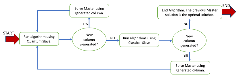
Figure 2. Progress of the quantum-assisted Algorithm

For every instance, we start the algorithm with the QSS as the slave. If the algorithm is able to generate a new column we use it to solve the master (RMP) and continue with the optimization loop using the QSS. Note that generating a new column here means that the MWIS solution found gives a positive $\sigma$ (as in equation (21)), hence violating (18). In case QSS is not able to generate a new column, we check whether the CSS can generate a new column. If the CSS is able the generate a new column, we solve the RMP using this new column and continue the optimization loop with the QSS. If even the CSS is unable to generate a new column, we have the optimal solution to the problem as the previous solution to the RMP obtained. This is explained diagrammatically in figure 2.

Using figure 2, we can modify Algorithm 1 to get Algorithm 2.

Input: Incompatibility graph $G(K,E)$

1 Define $R$ such that $R>\max\Gamma_{I}+1$

2 $\Lambda^{\prime}\leftarrow\emptyset$

3 while True do

4       Solve RMP and get primal dual couple $(x^{\prime},\mu^{\prime})$

5       for every model $v$ do

6            Solve SP using QSS

7             if $\sigma>0$ then

8                  Let the optimal solution be $I=(y_{I},c_{I})$.

9                   $\Lambda^{\prime}\leftarrow\Lambda^{\prime}\cup\{I\}$.

10             end if

11            

12       end for

13      

14       if $\Lambda^{\prime}$ has been modified then

15            continue

16       end if

17      else

18            for every model $v$ do

19                  Solve SP using CSS

20                   if $\sigma>0$ then

21                        Let the optimal solution be $I=(y_{I},c_{I})$.

22                         $\Lambda^{\prime}\leftarrow\Lambda^{\prime}\cup\{I\}$.

23                   end if

24                  

25             end for

26            if $\Lambda^{\prime}$ has been modified then

27                  continue

28             end if

29            else

30                  Current solution $x^{\prime}$ is the optimal solution

31                   break

32             end if

33            

34       end if

35      

36 end while

37

38

39Apply rounding algorithm to transform the relaxed solution $x^{\prime}$ into a binary one.

Algorithm 2 Quantum-assisted Column Generation algorithm for RMP

3. Experimental Results

In this section, we demonstrate experiments carried out using tours of sizes 32 and 64. Synthetic data was generated with start and end times of tours as well as sets of allowed vehicles for every tour. There are five different vehicle types and the cardinality of the set of allowed vehicles is 3. For simplicity, we do not generate location data. It can, however be added easily which will only change the density of the incompatibility graph. All runs of the quantum algorithm in this section are done using a quantum simulator.

Instance Size	No. of Qubits	Number of Instances	Mean $\%$ of Quantum Iterations
32	6	5	87.36
64	7	5	81.73

Table 1. Results for 32 and 64 Tours.

The number of successful quantum solves is compared to the total number of successful solves. A successful solve means that the QSS or CSS was able to generate a new column. In table 1, the number of quantum solves is shown as a percentage of the total number of solves, averaged over all the instances.

Figure 3 shows in detail a complete run of algorithm 2 for an instance of size 64. The first point of a plot is a gray point. This is a quick greedy solution to the problem and is the starting point of our algorithm. This ensures that we already have a decent solution to start with. As we go forward in the plots, we have blue and red points which signify the RMP solutions obtained using the QSS and the CSS respectively. Finally we have the black point which is the optimal point, where both the QSS and CSS were not able generate a new column.

In the above case, there are 16 iterations where the QSS was successful, 1 where QSS was unsuccessful and CSS was successful and 1 where both QSS and CSS were unsuccessful. Note, however, that for every iteration we called the QSS. Hence, there were a total of 18 QSS calls. Every QSS call requires 5 MWIS solutions (one for each vehicle type) each requiring around 300 expectation value measurements, hence the total number of expectation value measurements required were of the order of $10^{4}$. It was therefore not feasible to run the algorithm on a quantum computer since every expectation value measurement on an IBM quantum computer can take from a few seconds to a few hours, depending upon the wait time (or queue time). In addition we were limited to a size of 64 nodes for simulation since for 128 nodes and above, the simulation time was too long to carry out experiments. Here, the QPU might have significant time advantage over the simulators. However, larger sizes require the calculation of more expectation values in order to get even a feasible solution (an independent set). This further limits experiments on IBM QPUs. Implementation of the algorithm on other QPU systems is a viable road forward for such experiments.

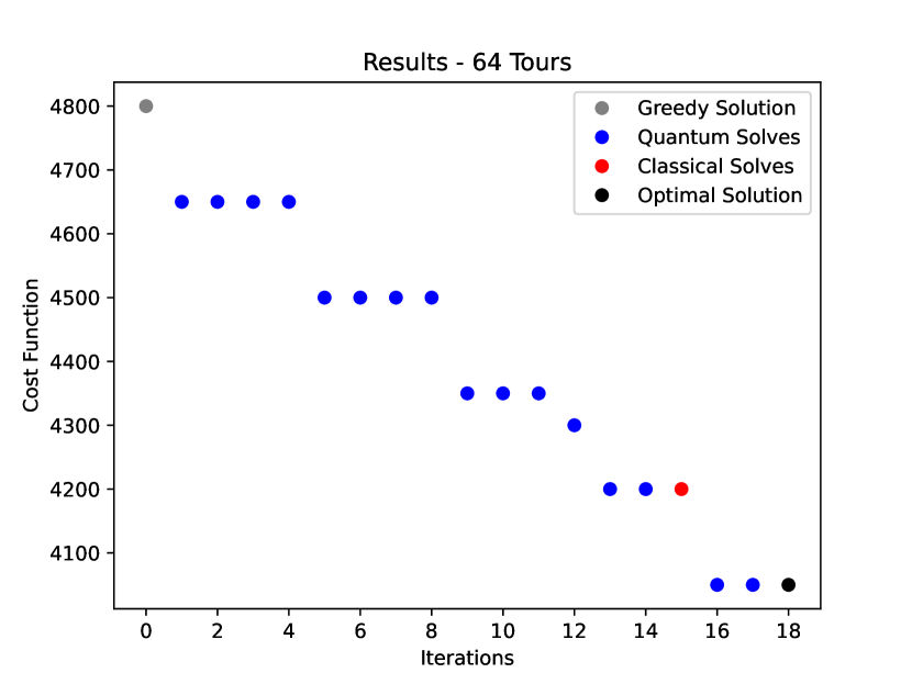
Figure 3. Full run of the algorithm for an instance of 64 tours.

4. Discussion and Conclusion

In this paper we have successfully demonstrated a quantum-assisted algorithm to solve the Fleet Conversion problem. This shows firstly the advantage of having an algorithm that scales logarithmically with the size of the problem. This trait helped us model problems of sizes that are well outside the realm of what other quantum variational algorithms can handle. Notably, our algorithm successfully handles instances that, albeit synthetic, represent real-world, non-trivial industrial problem sizes, which displays the potential utility of leveraging quantum computing for solving complex optimization problems.

Secondly, it demonstrates the possibility of harnessing quantum algorithms in conjunction with classical solvers rather than being in competition with them. If the problem is very resource intensive then instead of the using a full classical optimization, a part of the computation can be transferred to the quantum computer, potentially reducing required computational resources. The availability and efficiency of quantum hardware remain subjects of ongoing research.

Despite this uncertainty, notable advancements in the quantum hardware field in recent years, coupled with the qubit-efficiency of the demonstrated algorithm suggests that quantum-assisted algorithms may hold significant promise in the future.

- (1)
- Balinski and Tucker (1969) M. L. Balinski and A. W. Tucker. 1969. Duality Theory of Linear Programs: A Constructive Approach with Applications. SIAM Rev. 11, 3 (1969), 347–377. http://www.jstor.org/stable/2028941
- Barnhart et al. (1998) Cynthia Barnhart, Ellis L Johnson, George L Nemhauser, Martin WP Savelsbergh, and Pamela H Vance. 1998. Branch-and-price: Column generation for solving huge integer programs. Operations research 46, 3 (1998), 316–329.
- Bertsimas et al. (1999) Dimitris Bertsimas, Chungpiaw Teo, and Rakesh Vohra. 1999. On dependent randomized rounding algorithms. Operations Research Letters 24, 3 (1999), 105–114.
- Bittel and Kliesch (2021) Lennart Bittel and Martin Kliesch. 2021. Training variational quantum algorithms is np-hard. Physical Review Letters 127, 12 (2021), 120502. https://journals.aps.org/prl/abstract/10.1103/PhysRevLett.127.120502
- Callison and Chancellor (2022) Adam Callison and Nicholas Chancellor. 2022. Hybrid quantum-classical algorithms in the noisy intermediate-scale quantum era and beyond. Phys. Rev. A 106 (Jul 2022), 010101. Issue 1. https://doi.org/10.1103/PhysRevA.106.010101
- Calude et al. (2017) Cristian S Calude, Michael J Dinneen, and Richard Hua. 2017. QUBO formulations for the graph isomorphism problem and related problems. Theoretical Computer Science 701 (2017), 54–69.
- Cerezo et al. (2021) Marco Cerezo, Andrew Arrasmith, Ryan Babbush, Simon C Benjamin, Suguru Endo, Keisuke Fujii, Jarrod R McClean, Kosuke Mitarai, Xiao Yuan, Lukasz Cincio, et al. 2021. Variational quantum algorithms. Nature Reviews Physics 3, 9 (2021), 625–644. https://www.nature.com/articles/s42254-021-00348-9
- Chatterjee et al. (2023) Yagnik Chatterjee, Eric Bourreau, and Marko J Rančić. 2023. Solving various NP-Hard problems using exponentially fewer qubits on a Quantum Computer. arXiv preprint arXiv:2301.06978 (2023).
- Date et al. (2021) Prasanna Date, Davis Arthur, and Lauren Pusey-Nazzaro. 2021. QUBO formulations for training machine learning models. Scientific reports 11, 1 (2021), 10029.
- Demiriz et al. (2002) Ayhan Demiriz, Kristin P Bennett, and John Shawe-Taylor. 2002. Linear programming boosting via column generation. Machine Learning 46 (2002), 225–254.
- Desaulniers et al. (2006) Guy Desaulniers, Jacques Desrosiers, and Marius M Solomon. 2006. Column generation. Vol. 5. Springer Science & Business Media.
- Farhi et al. (2014) Edward Farhi, Jeffrey Goldstone, and Sam Gutmann. 2014. A quantum approximate optimization algorithm. arXiv preprint arXiv:1411.4028 (2014).
- Fuchs et al. (2021) Franz G Fuchs, Herman Øie Kolden, Niels Henrik Aase, and Giorgio Sartor. 2021. Efficient Encoding of the Weighted MAX k-CUT on a Quantum Computer Using QAOA. SN Computer Science 2, 2 (2021), 1–14. https://link.springer.com/article/10.1007/s42979-020-00437-z
- Gale et al. (1951) David Gale, Harold W Kuhn, and Albert W Tucker. 1951. Linear programming and the theory of games. Activity analysis of production and allocation 13 (1951), 317–335.
- Glover et al. (2019) Fred Glover, Gary Kochenberger, and Yu Du. 2019. Quantum Bridge Analytics I: a tutorial on formulating and using QUBO models. 4OR, Springer 17(4) (2019), 335–371. https://link.springer.com/article/10.1007/s10479-022-04634-2
- Hadfield et al. (2019) Stuart Hadfield, Zhihui Wang, Bryan O’Gorman, Eleanor G. Rieffel, Davide Venturelli, and Rupak Biswas. 2019. From the Quantum Approximate Optimization Algorithm to a Quantum Alternating Operator Ansatz. Algorithms 12, 2 (2019). https://doi.org/10.3390/a12020034
- Haidar et al. (2023) Mohammad Haidar, Marko J Rancic, Yvon Maday, and Jean-Philip Piquemal. 2023. Extension of the trotterized unitary coupled cluster to triple excitations. The Journal of Physical Chemistry A 127, 15 (2023), 3543–3550.
- Herman et al. (2022) Dylan Herman, Cody Googin, Xiaoyuan Liu, Alexey Galda, Ilya Safro, Yue Sun, Marco Pistoia, and Yuri Alexeev. 2022. A survey of quantum computing for finance. arXiv preprint arXiv:2201.02773 (2022).
- Herrman et al. (2021) Rebekah Herrman, Lorna Treffert, James Ostrowski, Phillip C Lotshaw, Travis S Humble, and George Siopsis. 2021. Globally optimizing QAOA circuit depth for constrained optimization problems. Algorithms 14, 10 (2021), 294. https://www.mdpi.com/1999-4893/14/10/294
- Larkin et al. (2022) Jason Larkin, Matías Jonsson, Daniel Justice, and Gian Giacomo Guerreschi. 2022. Evaluation of QAOA based on the approximation ratio of individual samples. Quantum Science and Technology (2022). https://iopscience.iop.org/article/10.1088/2058-9565/ac6973
- Lubasch et al. (2020) Michael Lubasch, Jaewoo Joo, Pierre Moinier, Martin Kiffner, and Dieter Jaksch. 2020. Variational quantum algorithms for nonlinear problems. Physical Review A 101, 1 (2020), 010301. https://journals.aps.org/pra/abstract/10.1103/PhysRevA.101.010301
- Martin et al. (2022) Baptiste Anselme Martin, Pascal Simon, and Marko J Rančić. 2022. Simulating strongly interacting Hubbard chains with the variational Hamiltonian ansatz on a quantum computer. Physical Review Research 4, 2 (2022), 023190.
- Mehic et al. (2020) Miralem Mehic, Marcin Niemiec, Stefan Rass, Jiajun Ma, Momtchil Peev, Alejandro Aguado, Vicente Martin, Stefan Schauer, Andreas Poppe, Christoph Pacher, et al. 2020. Quantum key distribution: a networking perspective. ACM Computing Surveys (CSUR) 53, 5 (2020), 1–41.
- Mehrotra and Trick (1996) Anuj Mehrotra and Michael A Trick. 1996. A column generation approach for graph coloring. informs Journal on Computing 8, 4 (1996), 344–354.
- Moll et al. (2018) Nikolaj Moll, Panagiotis Barkoutsos, Lev S Bishop, Jerry M Chow, Andrew Cross, Daniel J Egger, Stefan Filipp, Andreas Fuhrer, Jay M Gambetta, Marc Ganzhorn, et al. 2018. Quantum optimization using variational algorithms on near-term quantum devices. Quantum Science and Technology 3, 3 (2018), 030503. https://iopscience.iop.org/article/10.1088/2058-9565/aab822
- Nakanishi et al. (2020) Ken M Nakanishi, Keisuke Fujii, and Synge Todo. 2020. Sequential minimal optimization for quantum-classical hybrid algorithms. Physical Review Research 2, 4 (2020), 043158. https://journals.aps.org/prresearch/abstract/10.1103/PhysRevResearch.2.043158
- Nielsen and Chuang (2011) Michael A. Nielsen and Isaac L. Chuang. 2011. Quantum Computation and Quantum Information: 10th Anniversary Edition. Cambridge University Press. https://www.amazon.com/Quantum-Computation-Information-10th-Anniversary/dp/1107002176?SubscriptionId=AKIAIOBINVZYXZQZ2U3A&tag=chimbori05-20&linkCode=xm2&camp=2025&creative=165953&creativeASIN=1107002176
- Orús et al. (2019) Román Orús, Samuel Mugel, and Enrique Lizaso. 2019. Quantum computing for finance: Overview and prospects. Reviews in Physics 4 (2019), 100028.
- Papalitsas et al. (2019) Christos Papalitsas, Theodore Andronikos, Konstantinos Giannakis, Georgia Theocharopoulou, and Sofia Fanarioti. 2019. A QUBO model for the traveling salesman problem with time windows. Algorithms 12, 11 (2019), 224.
- Peruzzo et al. (2014) Alberto Peruzzo, Jarrod McClean, Peter Shadbolt, Man-Hong Yung, Xiao-Qi Zhou, Peter J Love, Alán Aspuru-Guzik, and Jeremy L O’brien. 2014. A variational eigenvalue solver on a photonic quantum processor. Nature communications 5, 1 (2014), 1–7. https://www.nature.com/articles/ncomms5213
- Preskill (2018) John Preskill. 2018. Quantum Computing in the NISQ era and beyond. Quantum 2 (2018), 79. https://doi.org/10.22331/q-2018-08-06-79
- Preskill (2021) John Preskill. 2021. Quantum computing 40 years later. arXiv (2021). https://www.amazon.science/publications/quantum-computing-40-years-later
- Rančić (2023) Marko J Rančić. 2023. Noisy intermediate-scale quantum computing algorithm for solving an n-vertex MaxCut problem with log (n) qubits. Physical Review Research 5, 1 (2023), L012021.
- Scarani et al. (2009) Valerio Scarani, Helle Bechmann-Pasquinucci, Nicolas J Cerf, Miloslav Dušek, Norbert Lütkenhaus, and Momtchil Peev. 2009. The security of practical quantum key distribution. Reviews of modern physics 81, 3 (2009), 1301.
- Stokes et al. (2020) James Stokes, Josh Izaac, Nathan Killoran, and Giuseppe Carleo. 2020. Quantum natural gradient. Quantum 4 (2020), 269. https://quantum-journal.org/papers/q-2020-05-25-269/
- Wilhelm (2001) Wilbert E Wilhelm. 2001. A technical review of column generation in integer programming. Optimization and Engineering 2 (2001), 159–200.
- Zhou et al. (2020) Leo Zhou, Sheng-Tao Wang, Soonwon Choi, Hannes Pichler, and Mikhail D Lukin. 2020. Quantum approximate optimization algorithm: Performance, mechanism, and implementation on near-term devices. Physical Review X 10, 2 (2020), 021067. https://link.aps.org/doi/10.1103/PhysRevX.10.021067