A Geometric Perspective on Autoencoders

Abstract

This paper presents the geometric aspect of the autoencoder framework, which, despite its importance, has been relatively less recognized. Given a set of high-dimensional data points that approximately lie on some lower-dimensional manifold, an autoencoder learns the manifold and its coordinate chart, simultaneously. This geometric perspective naturally raises inquiries like “Does a finite set of data points correspond to a single manifold?” or “Is there only one coordinate chart that can represent the manifold?”. The responses to these questions are negative, implying that there are multiple solution autoencoders given a dataset. Consequently, they sometimes produce incorrect manifolds with severely distorted latent space representations. In this paper, we introduce recent geometric approaches that address these issues.

1 Introduction

Observations from real-world problems are often high-dimensional, i.e., a large number of variables is needed to numerically represent the observed data. Manifold hypothesis assumes that high-dimensional data lie approximately on some lower-dimensional manifold, suggesting that a data set that appears to initially require many variables to describe can actually be described by a comparatively small number of variables; below shows one intuitive example.

Example 1.1.

Rotating face image manifold. There is a sequence of pictures of a person turning his head from left to right as shown in Figure 1, where each image size is $3\times 728\times 1280$. These images can be initially viewed as elements of the high-dimensional image data space $\mathbb{R}^{3\times 728\times 1280}$, however, they clearly do not fill up the entire image space, but rather form a lower-dimensional subspace. We need only one variable to represent these images, e.g., the angle of the person’s head, meaning that the set of images can be interpreted as lying on a one-dimensional subspace or a curve as shown in Figure 1.

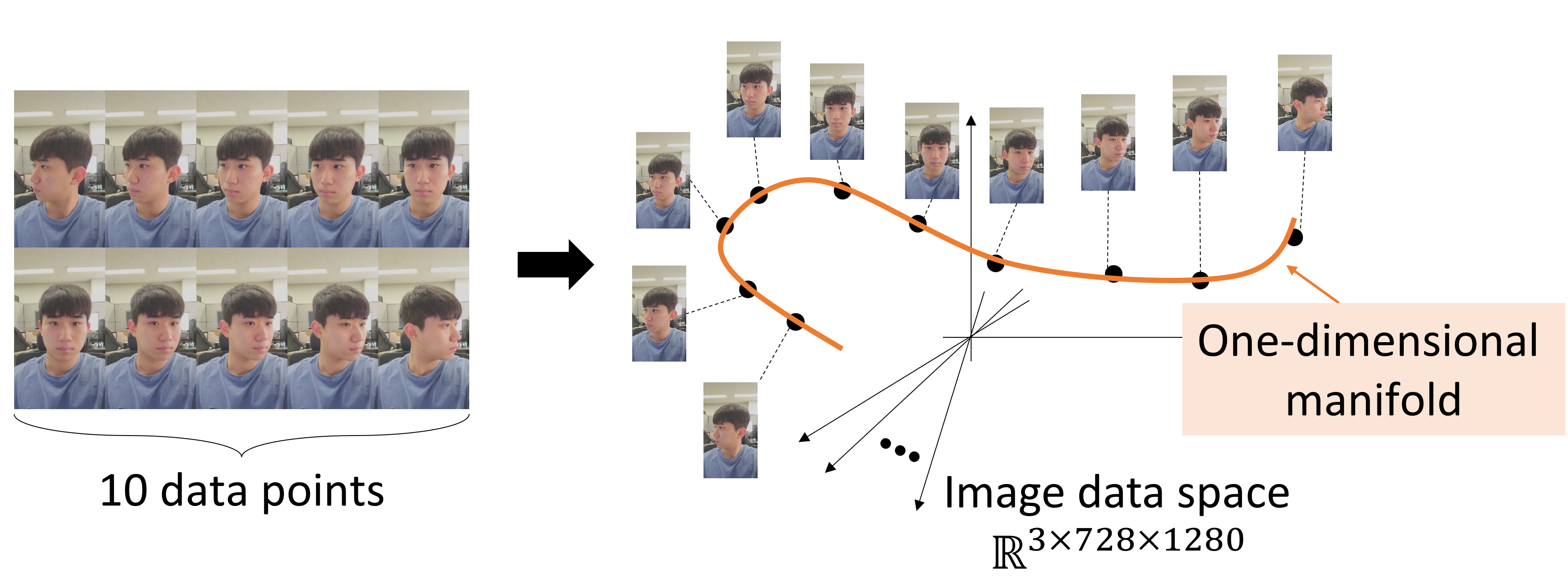
Figure 1: A set of face images, where a person turns his head from left to right, approximately lie on a one-dimensional manifold or a curve.

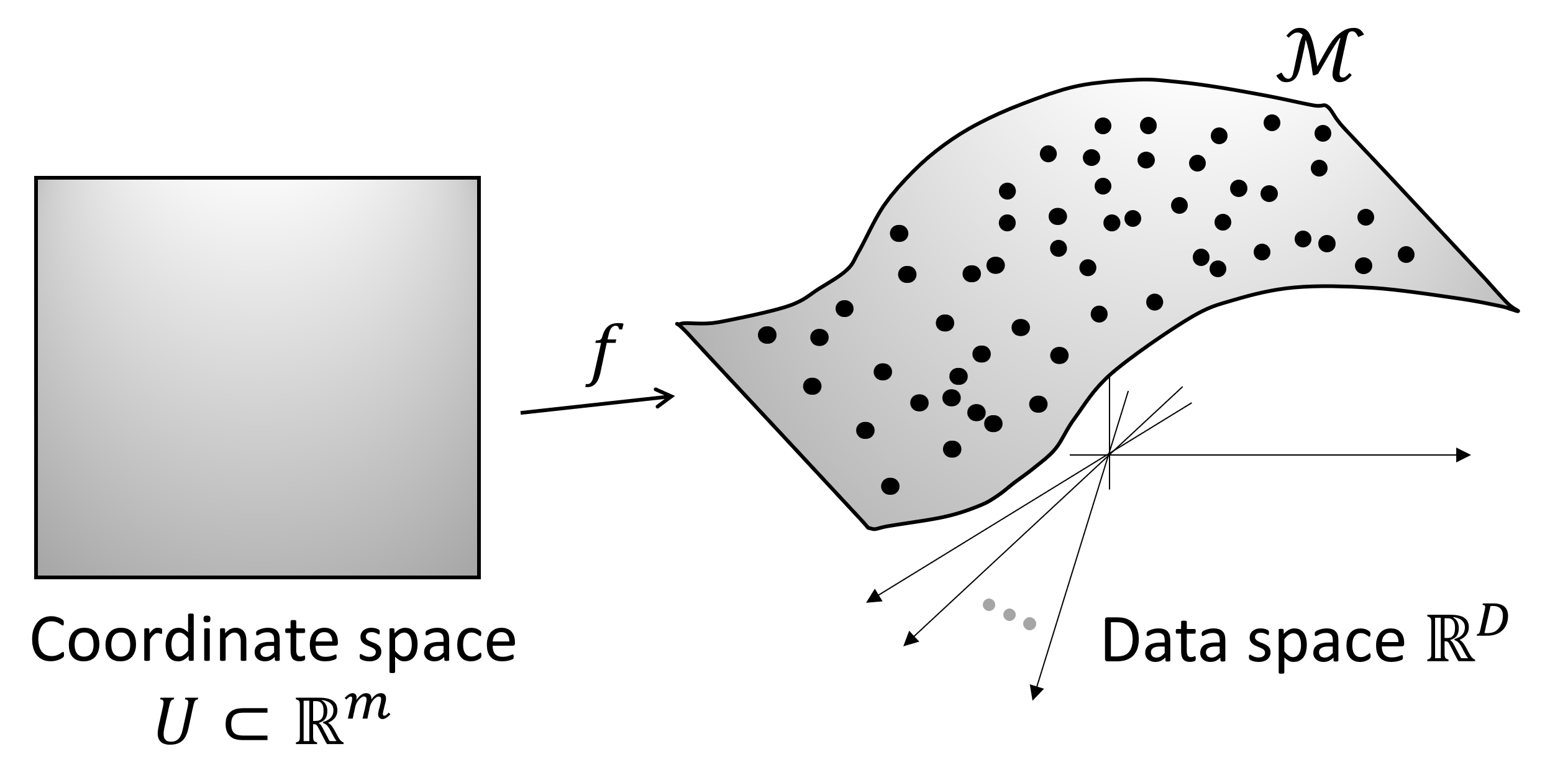
Figure 2: An illustration of the manifold ${\cal M}$ and coordinate chart $f:U\to{\cal M}$.

Under the manifold hypothesis, suppose a finite set of data points $\{x_{i}\in\mathbb{R}^{D}\}$ approximately lie on some manifold of dimension $m<D$, denoted by ${\cal M}$. In other words, the support of the underlying data distribution $p_{X}(x)$ is contained in ${\cal M}$, i.e., $\text{supp}(p_{X})\subset{\cal M}$. Then, the manifold representation learning problem consists of the following two components: (i) identifying the manifold ${\cal M}\subset\mathbb{R}^{D}$ and (ii) finding a coordinate chart, i.e., a continuous and invertible map $f:U\to{\cal M}$ for some subset $U\subset\mathbb{R}^{m}$ (see Figure 2).

The autoencoder framework provides an effective way of learning the manifold and coordinate chart simultaneously (Kramer, 1991), together with the deep learning techniques used for approximating arbitrary complex functions (LeCun et al., 2015). The core idea is to learn two neural networks, an encoder $g_{\phi}:\mathbb{R}^{D}\to\mathbb{R}^{m}$ and a decoder $f_{\theta}:\mathbb{R}^{m}\to\mathbb{R}^{D}$, in a way that the composition of them reconstructs all the given data points $x_{i}\in\mathbb{R}^{D}$, i.e., $f\circ g(x_{i})\approx x_{i}$, by solving the following reconstruction loss minimization problem:

$$\min_{\theta,\phi}\sum_{i=1}^{N}\|x_{i}-f_{\theta}(g_{\phi}(x_{i}))\|^{2}.$$ (1)

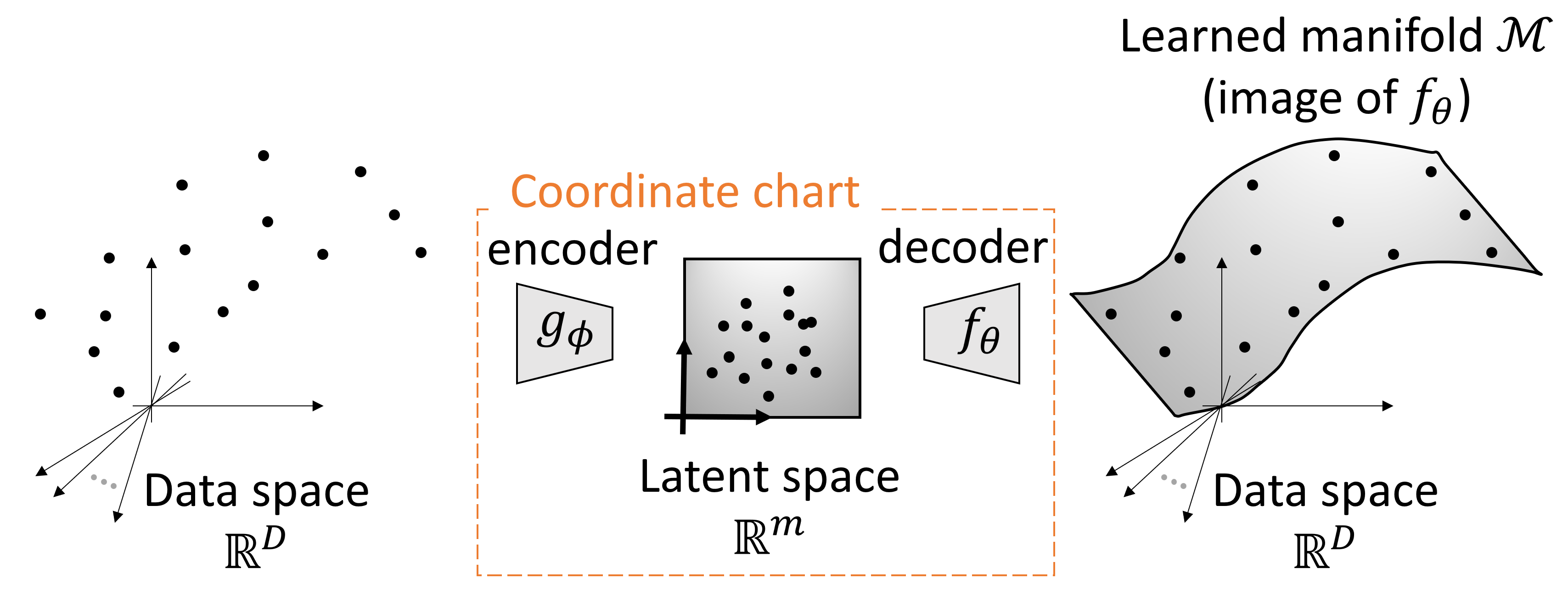
Figure 3: An autoencoder-based simultaneous manifold and coordinate chart learning

Provided that the loss approaches near zero, the data points become to lie on the image of the decoder $f_{\theta}$, i.e., $x_{i}\in\text{image}(f_{\theta})$. Under some suitable conditions, the image of the decoder is a differentiable manifold, and it can be seen that $f_{\theta}$ has learned the manifold ${\cal M}$:

Remark 1.1.

If $f_{\theta}:\mathbb{R}^{m}\to\mathbb{R}^{D}$ is a smooth injection and its Jacobian is full rank, then the image of $f_{\theta}$ is a differentiable manifold embedded in $\mathbb{R}^{D}$.

The encoder $g_{\phi}$ maps the data points $x_{i}$ to some low-dimensional latent vectors in $\mathbb{R}^{m}$, and the subset $U$ can be found by fitting a probability density function to $\{g_{\phi}(x_{i})\}$ and taking its support.

For ease of discussion, throughout, we will assume that the manifold ${\cal M}$ is homeomorphic to $\mathbb{R}^{m}$, i.e., ${\cal M}$ is continuously deformable to $\mathbb{R}^{m}$, and consider the entire image of $f_{\theta}:\mathbb{R}^{m}\to\mathbb{R}^{D}$ as the learned manifold (or decoded manifold); see Figure 3. We denote by ${\cal M}$ this decoded manifold by a slight abuse of notation, and the manifold is said to be explicitly parametrized by $f_{\theta}$. Then, informally, we can view $g_{\phi}:{\cal M}\to\mathbb{R}^{m}$ as an approximate inverse of $f_{\theta}:\mathbb{R}^{m}\to{\cal M}$. The encoder and decoder with the latent space $\mathbb{R}^{m}$ together take the role of the coordinate chart.

In vanilla autoencoders, there are two fundamental issues that we aim to address: (i) they often learn incorrect manifolds that overfit to training data or have the wrong local connectivity and geometry, and (ii) they learn geometrically distorted latent representations where geometric quantities such as the lengths, angles, and volumes in the data manifold are not preserved. Below, we will take a closer look at the following issues one by one.

1.1 Wrong Manifold

In the traditional autoencoder training setting, we are given a set of finite data points $\{x_{i}\in\mathbb{R}^{D}\}_{i=1}^{N}$. Assuming the data points are clean and perfectly lie on the ground-truth data manifold $\mathcal{M}$, the primary condition for a correct coordinate system $f:\mathbb{R}^{m}\to\mathbb{R}^{D}$ to satisfy is the following:

$$x_{i}\in\mathcal{M}\subset\mathbb{R}^{D}\text{ for all }i\Longleftrightarrow x_{i}\in\text{image}(f)\text{ for all }i.$$ (2)

However, finding such a map $f$ is fundamentally ill-posed, meaning that there are infinitely many mappings $f$ that satisfy the above condition. For example, as shown in Figure 4, assume that there exists a ground-truth one-dimensional manifold embedded in the two-dimensional data space and we are given a set of finite two-dimensional data points (blue points). There are many manifolds (orange manifolds) where the given data points perfectly lie; thus, we cannot specify the solution manifold without further assumptions on the manifold or decoder $f$.

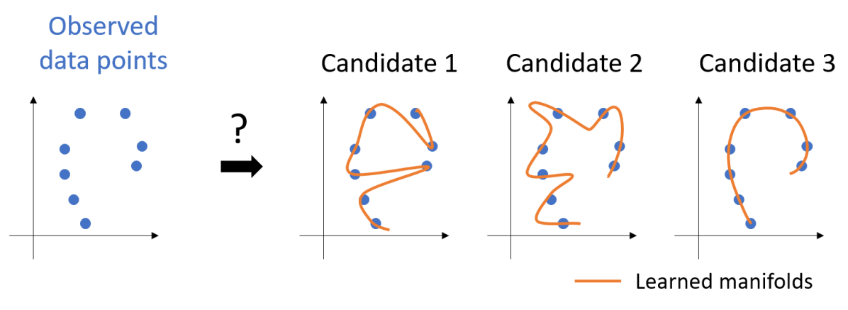
Figure 4: An illustration of the fundamental wrong manifold issue in autoencoder-based manifold learning. Given blue data points, there are many manifolds where the given data points perfectly lie.

1.2 Distorted Latent Space

Given a ground-truth data manifold $\mathcal{M}$, the problem of finding a coordinate system for $\mathcal{M}$ is again fundamentally ill-posed because there exist infinitely many coordinate systems. For example, if $f:\mathbb{R}^{m}\to\mathcal{M}$ is one coordinate system, then for any continuous and invertible map $h:\mathbb{R}^{m}\to\mathbb{R}^{m}$ the composition map $f\circ h^{-1}:\mathbb{R}^{m}\to\mathcal{M}$ is also another coordinate system (Figure 5). Recall the reconstruction error objective function in the vanilla autoencoder $\sum_{i}\|x_{i}-f\circ g(x_{i})\|^{2}$, if $f^{*}$ and $g^{*}$ are solutions, then for any continuous and invertible map $h:\mathbb{R}^{m}\to\mathbb{R}^{m}$ the composition maps $f^{*}\circ h^{-1}$ and $h\circ g^{*}$ are also solutions. Therefore, we cannot favor one coordinate system over the others without further assumptions on the mappings.

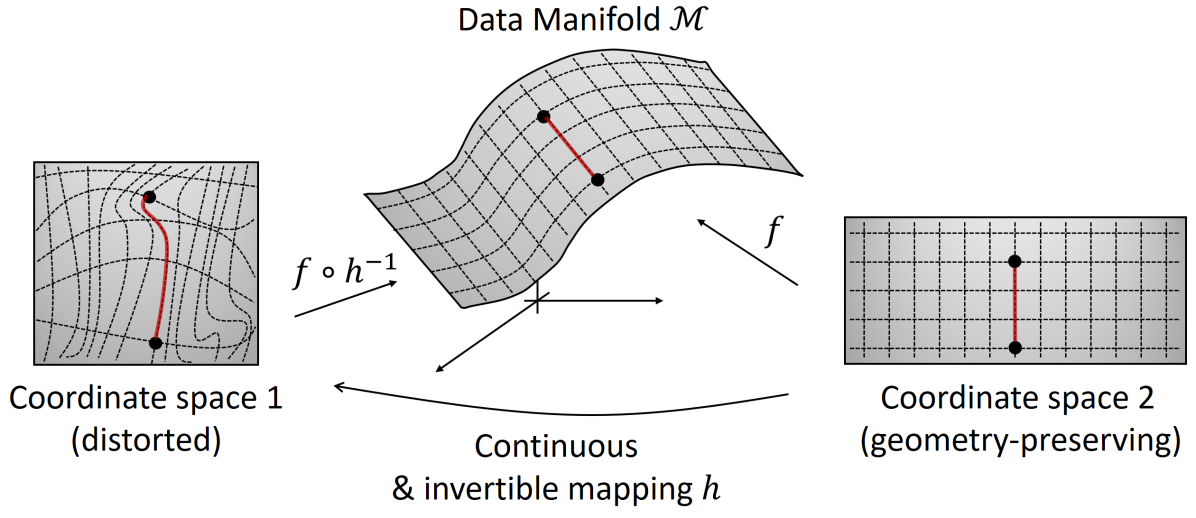
Figure 5: There are many coordinate systems for a data manifold $\mathcal{M}$; some produce geometrically distorted coordinate spaces.

This is closely related to the classical map-making problem, i.e., making a map of the earth, by finding a mapping from the surface of the earth approximated by a two-dimensional sphere $S^{2}$ to a two-dimensional Cartesian plane $\mathbb{R}^{2}$ (Figure 6). As shown in Figure 7, a wide variety of maps of the earth exist, each of which is based on different projection methods. In general, maps that are arbitrarily distorted are not preferred, rather it is designed to preserve specific intrinsic geometric quantities defined based on the purpose of the map. For example, the Mercator projection preserves angles while the areas are distorted, and the Gall-Peters map preserves areas although the shapes are distorted (Figure 8).

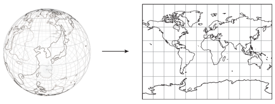
Figure 6: Map-making: finding a mapping from a sphere to a Cartesian plane, adopted from Figure 1.5 in (Jang, 2019).

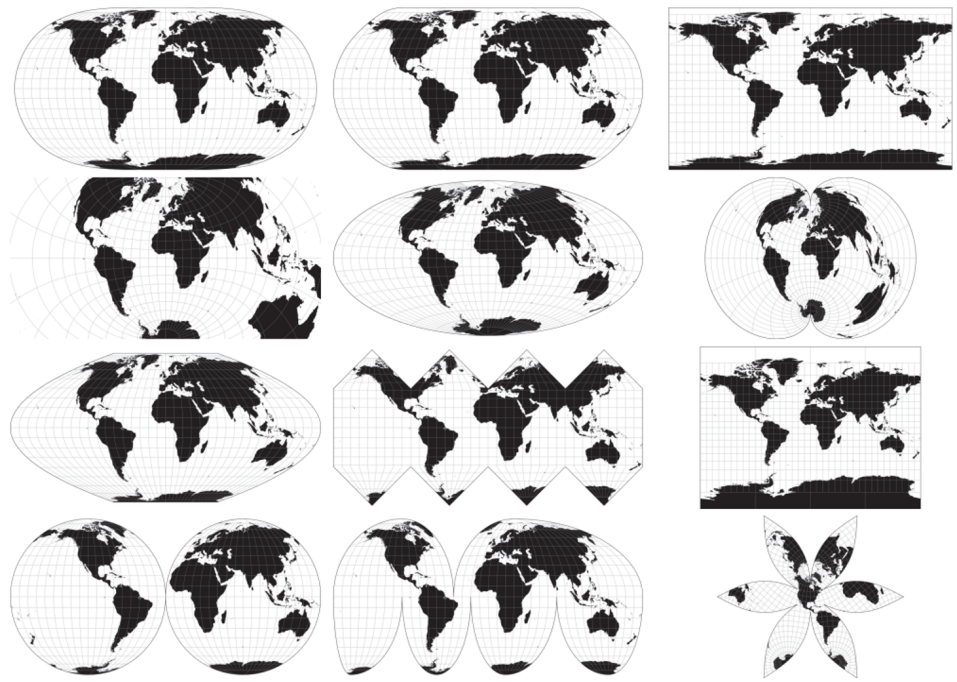
Figure 7: Maps of the earth, adopted from Figure 1.6 in (Jang, 2019).

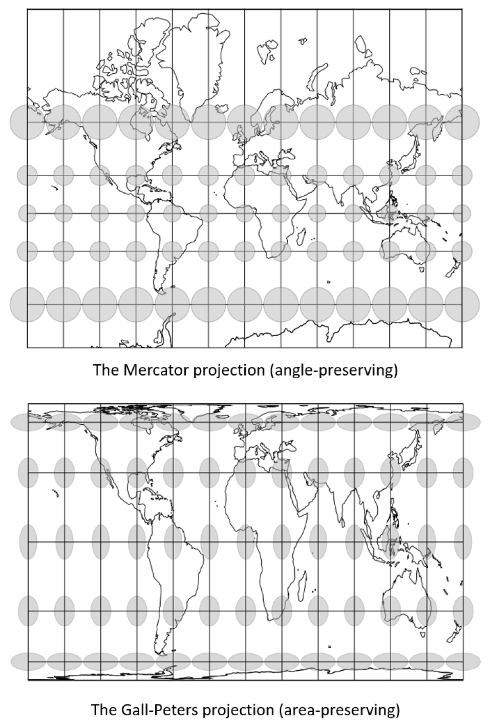
Figure 8: Two examples of maps of the earth, adopted from Figure 1.7 in (Jang, 2019).

In this paper, we introduce recent geometric regularization methods that attempt to resolve these two issues. Before that, in section 2, we introduce some geometric preliminaries required to understand the subsequent sections. Section 3.1, which is based on (Lee et al., 2021), introduces a method to resolve the wrong manifold issue by using additional information, a priori constructed neighborhood graph. We regularize the geometry and connectivity of the learned manifold to be close to those of the given neighborhood graph. Section 3.2, which is based on (Lee & Park, 2023), attempts to minimize the curvature of the learned manifold, prioritizing smooth manifolds over curved ones. Section 3.3, which is based on (Lee et al., 2022b), introduces a method to resolve the distorted latent space issue, by trying to regularize the decoder to be close to a geometry-preserving mapping. Besides ours, we note that there are many other autoencoder regularization methods developed from different perspectives (Arvanitidis et al., 2018; Shao et al., 2018; Rifai et al., 2011; Kingma & Welling, 2013; Tolstikhin et al., 2017; Makhzani et al., 2015; Vincent et al., 2010; Chen et al., 2020; Higgins et al., 2016; Jang et al., 2022; Chen et al., 2021; Duque et al., 2020).

2 Geometric Preliminaries

Throughout, we denote the decoder by $f:\mathbb{R}^{m}\to\mathbb{R}^{D}$ such that $z\mapsto x=f(z)$, and consider its image as an $m$-dimensional differentiable manifold ${\cal M}$ embedded in $\mathbb{R}^{D}$. The space $\mathbb{R}^{D}$ is called the ambient space. In this section, we discuss various geometric quantities of ${\cal M}$ and $f$. We will denote the Jacobian of $f$ by $J_{f}\in\mathbb{R}^{D\times m}$.

2.1 Tangent Space and Riemannian Metric

The decdoer Jacobian $J_{f}(z)$ spans the tangent space of the manifold ${\cal M}$ attached at $x=f(z)$ – where we consider $x\in{\cal M}$ as an origin of the tangent vector space $T_{x}{\cal M}$ –, i.e, $T_{x}{\cal M}=\{x+J_{f}(z)v\ |\ v\in\mathbb{R}^{m}\}\subset\mathbb{R}^{D}$. The $m$ column vectors in the Jacobian matrix $J_{f}(z)\in\mathbb{R}^{D\times m}$ can be viewed as a set of linearly independent basis vectors for the tangent space.

We can give a geometric structure to a differentiable manifold ${\cal M}$ by assigning a Riemannian metric, i.e., inner products $\{\langle\cdot,\cdot\rangle_{x}\}$ for the tangent spaces $\{T_{x}{\cal M}\}$ that smoothly change with respect to $x$. One natural way to define the metric for ${\cal M}$ is to project the ambient space Riemannian metric to ${\cal M}$. Let $H(x)\in\mathbb{R}^{D\times D}$ – which is a positive-definite matrix – be a Riemannian metric for the ambient space. Then, the projected metric to the embedded manifold ${\cal M}$ is defined as follows: for two tangent vectors $v,w\in T_{x}{\cal M}\subset\mathbb{R}^{D}$, $\langle v,w\rangle_{x}:=v^{T}H(x)w$.

Given a decoder (or a coordinate chart), this projected metric can be expressed in local coordinates as $m\times m$ positive-definite matrices. Consider arbitrary two smooth curves $z_{1}(t)$ and $z_{2}(t)$ in $\mathbb{R}^{m}$ that intersect at $t=0$, i.e., $z=z_{1}(0)=z_{2}(0)$, and their corresponding curves in ${\cal M}$ denoted by $x_{1}(t)=f(z_{1}(t))$ and $x_{2}(t)=f(z_{2}(t))$. Differentiating both sides, we get $\dot{x}_{1}=J_{f}(z)\dot{z}_{1}$ and $\dot{x}_{2}=J_{f}(z)\dot{z}_{2}$. Note that $\dot{x}_{1}$ and $\dot{x}_{2}$ are two tangent vectors in $T_{x}{\cal M}$, and we can compute their inner product using the projected metric $\langle\dot{x}_{1},\dot{x}_{2}\rangle_{x}$; then, we get the following equality:

$$\dot{x}_{1}^{T}H(x)\dot{x}_{2}=\dot{z}_{1}^{T}J_{f}(z)^{T}H(f(z))J_{f}(z)\dot{z}_{2}.$$ (3)

The matrix $J_{f}(z)^{T}H(f(z))J_{f}(z)$ is an $m\times m$ positive-definite matrix, which defines inner products between $\dot{z}_{1}$ and $\dot{z}_{2}$ for arbitrary curves $z_{1}(t),z_{2}(t)$ in the latent space. It is called either a pull-back metric of $H$ by $f$, a coordinate representation of the projected metric of $H$ to ${\cal M}$, or sometimes a latent Riemannian metric.

Now that we have defined the geometry of ${\cal M}$ with the Riemannian metric, we can compute the length of a curve in ${\cal M}$. Let $x(t),t\in[0,1]$ be a smooth curve in ${\cal M}$ and $z(t)$ be its coordinate representation, i.e., $x(t)=f(z(t))$. Given the projected metric $H$ to ${\cal M}$, the length of the curve can be computed by using the pull-back metric as follows:

$$\text{Len}(x(t)):=\int_{0}^{1}\sqrt{\dot{z}^{T}J_{f}(z)^{T}H(f(z))J_{f}(z)\dot{z}}\ dt.$$ (4)

And, the energy of the curve is defined as

$$\text{Energy}(x(t)):=\int_{0}^{1}\dot{z}^{T}J_{f}(z)^{T}H(f(z))J_{f}(z)\dot{z}\ dt.$$ (5)

Given two points in ${\cal M}$, a minimal geodesic is defined as the energy-minimizing curve and minimal geodesic distance is defined as its length. Previous works (Arvanitidis et al., 2018; Shao et al., 2018; Arvanitidis et al., 2020) computed geodesics and geodesic distances by solving geodesic equations or energy minimization problems.

2.2 Manifold Curvature Measures

This section explains the extrinsic curvature measure proposed in (Lee & Park, 2023). Recall that the curvature of a curve is a measure of the local rate of change of the tangent vector: straight lines have zero curvature, while circles have constant curvatures. In the same way, the curvature of a manifold ${\cal M}$ in $\mathbb{R}^{D}$ can be defined as a measure of the local rate of change of the tangent space $T_{x}{\cal M}$.

The tangent space $T_{x}{\cal M}$ corresponds to the range of the Jacobian, and we may choose $J_{f}(z)$ as a numerical representation of the tangent space. However, it is not coordinate invariant and thus not geometrically well-defined: given a coordinate transformation $z\mapsto\tilde{z}(z)$ and $f(z)=\tilde{f}(\tilde{z}(z))$, $J_{f}=\frac{\partial f}{\partial z}\mapsto J_{\tilde{f}}=J_{f}\frac{\partial z}{\partial\tilde{z}}$.

Instead, we can represent the tangent space $T_{x}{\cal M}$ with a $D\times D$ orthogonal projection matrix in a coordinate-invariant way:

$$T_{x}{\cal M}=\text{range}(J_{f}(J_{f}^{T}J_{f})^{-1}J_{f}^{T}),$$ (6)

where $J_{f}(J_{f}^{T}J_{f})^{-1}J_{f}^{T}$ is the orthogonal projection matrix that projects a $D$-dimensional vector in $\mathbb{R}^{D}$ to $T_{x}{\cal M}$; this representation is invariant under the coordinate transformations:

Proposition 2.1.

Given a coordinate transformation $z\mapsto\tilde{z}(z)$, $J_{f}(J_{f}^{T}J_{f})^{-1}J_{f}^{T}=J_{\tilde{f}}(J_{\tilde{f}}^{T}J_{\tilde{f}})^{-1}J_{\tilde{f}}^{T}$.

There is one-to-one correspondence between the set of $D\times D$ orthogonal projection matrices of rank $m$ and the set of $m$-dimensional linear subspaces in $\mathbb{R}^{D}$, which again validates our choice of the orthogonal projection matrix representation. More formally, this argument can be made by using the theory of the Grassmann manifold; see (Lee & Park, 2023).

We denote the orthogonal projection matrix representation of $T_{x}{\cal M}$ by $\hat{T}=J_{f}(J_{f}^{T}J_{f})^{-1}J_{f}^{T}$. Given a curve $x(t)=f(z(t))\in{\cal M}$, the local change of the tangent space along the curve can then be expressed in local coordinates as

$$\frac{d\hat{T}}{dt}=\sum_{i=1}^{m}\frac{\partial\hat{T}}{\partial z^{i}}\ \dot{z}^{i}\in\mathbb{R}^{D\times D}.$$ (7)

And, its Frobenius norm is

$$\|\frac{d\hat{T}}{dt}\|_{F}^{2}=\sum_{i=1}^{m}\sum_{j=1}^{m}\text{Tr}(\frac{d\hat{T}}{dz^{i}}^{T}\frac{d\hat{T}}{dz^{j}})\dot{z}^{i}\dot{z}^{j};$$ (8)

the resulting quadratic form is

$$\|\dot{\hat{T}}\|_{F}^{2}\ dt=\sum_{i=1}^{m}\sum_{j=1}^{m}c_{ij}(z)dz^{i}dz^{j}=dz^{T}C(z)dz,$$ (9)

where $dz=(dz^{1},\ldots,dz^{m})$, and the matrix $C(z)\in\mathbb{R}^{m\times m}$ is defined to be $c_{ij}(z)=\text{Tr}(\frac{d\hat{T}}{dz^{i}}^{T}\frac{d\hat{T}}{dz^{j}})$, which we call the extrinsic curvature form.

Given the pull-back Riemannian metric $J^{T}_{f}HJ_{f}$, we can define a local extrinsic curvature measure of ${\cal M}\subset\mathbb{R}^{D}$ at $z$ as follows:

$$\text{Tr}((J_{f}^{T}HJ_{f})^{-1}C)=\sum_{i,j}(J_{f}^{T}HJ_{f})^{-1}_{ij}\text{Tr}(\frac{d\hat{T}}{dz^{i}}\frac{d\hat{T}}{dz^{j}}),$$ (10)

which is a Dirichlet energy of the mapping between the Riemannian manifold ${\cal M}$ and the Grassmann manifold; see (Lee & Park, 2023). This curvature measure is geometrically well-defined since it is invariant under the coordinate transformations:

Proposition 2.2.

Given a coordinate transformation $z\mapsto\tilde{z}(z)$, $\text{Tr}((J_{f}^{T}HJ_{f})^{-1}C)$ is invariant.

This is a local measure at $z\in\mathbb{R}^{m}$, and to define a global measure, we can either integrate the local curvature measure over some regions or compute the expectation over some probability measure in $\mathbb{R}^{m}$.

This section exclusively deals with the extrinsic curvature measure that we have proposed. Although not introduced here, there are well-developed theories of intrinsic curvatures of Riemannian manifolds such as Riemann curvature, Ricci curvature, and scalar curvature; we refer to (Do Carmo & Flaherty Francis, 1992; Fecko, 2006) for those who are interested. In (Lee & Park, 2023), algorithms for both extrinsic and intrinsic curvatures have been developed.

2.3 A Hierarchy of Geometry-Preserving Mappings and Distortion Measures

This section introduces a hierarchy of geometry-preserving mappings and coordinate-invariant distortion measures in (Jang et al., 2020; Lee et al., 2022b). For simplicity, here we will restrict our attention to the decoder $f:\mathbb{R}^{m}\to\mathbb{R}^{D}$; formulations for mappings between general manifolds can be found in the original papers. Throughout, we will assume that both latent and data spaces are Riemannian manifolds, where the latent space $\mathbb{R}^{m}$ is assigned the identity metric (i.e., Euclidean space), and the ambient data space is assigned the Riemannian metric $H(x)$.

2.3.1 A Hierarchy of Geometry-Preserving Mappings

At the top of the hierarchy, an isometry is a mapping between two spaces that preserves distances and angles everywhere. For a linear mapping between two vector spaces equipped with inner products, an isometry preserves the inner product everywhere. In the case of a mapping between Riemannian manifolds, $f$ is an isometry if

$$I=J_{f}(z)^{T}H(f(z))J_{f}(z)\>\>\>\forall z\in\mathbb{R}^{m}.$$ (11)

This equality condition is derived from the requirement that the $\text{Len}(x(t))$ in ${\cal M}$ expressed in the equation (4) must be equal to the $\text{Len}(z(t))=\int_{0}^{1}\sqrt{\dot{z}^{T}\dot{z}}\ dt$ in $\mathbb{R}^{m}$ for all curve $x(t)\in{\cal M}$.

Sometimes, requiring a map $f$ to be an isometry can be overly restrictive; preserving only angles may be sufficient. A conformal map is a mapping that preserves angles but not necessarily distances. Mathematically, $f$ is conformal (or angle-preserving) if

$$I=c(z)J_{f}(z)^{T}H(f(z))J_{f}(z)\>\>\>\forall z\in\mathbb{R}^{m},$$ (12)

for some positive function $c:\mathbb{R}^{m}\to\mathbb{R}$. The positive function is called the conformal factor.

A conformal map with a constant conformal factor, i.e., one in which $c(z)$ is constant, sits one level below the isometric mapping and is defined formally as any mapping $f$ for which a positive scalar constant $c$ satisfying

$$I=cJ_{f}(z)^{T}H(f(z))J_{f}(z)\>\>\>\forall z\in\mathbb{R}^{m}$$ (13)

can be found. Such a map not only preserves angles but also scaled distances; for this reason, this mapping is referred to as the scaled isometry.

2.3.2 Distortion measures

We begin by introducing another equivalent characterization of the isometry condition in (11). $f$ is an isometry if all the eigenvalues of $J_{f}^{T}(z)H(f(z))J_{f}(z)$ are equal to 1 for all $z\in\mathbb{R}^{m}$. Then, denoting the eigenvalues by $\{\lambda_{i}(z)\}$, we can define a local distortion measure of $f$, which measures how far the mapping $f$ from being a local isometry, as follows:

$$\sum_{i=1}^{m}(1-\lambda_{i}(z))^{2}.$$ (14)

This local measure can be integrated over some probability measure $\nu$ in $\mathbb{R}^{m}$ to define a global distortion measure:

$$\int_{\mathbb{R}^{m}}\sum_{i=1}^{m}(1-\lambda_{i}(z))^{2}\ d\nu(z).$$ (15)

Since the influence of the measure is limited to the support of $\nu$, if the global distortion measure of $f$ is zero, then $f$ is an isometry with respect to the support of $\nu$. For simplicity, we omit the expression ‘with respect to the support of $\nu$’ whenever it is clear from the context.

One may naively want to consider $\|I-J_{f}^{T}HJ_{f}\|_{F}^{2}$ as a local distortion measure, but such a measure is not coordinate-invariant. Our distortion measure defined with the eigenvalues is coordinate-invariant and thus is geometrically well-defined. We refer to (Lee et al., 2022b; Jang et al., 2020) for a general strategy of constructing coordinate-invariant functionals on Riemannian manifolds and general formulations of coordinate-invariant distortion measures.

For a scaled isometry, the condition (13) is equivalent to $\lambda_{i}(z)=c$ for some positive scalar $c$ and for all $z\in\mathbb{R}^{m}$. A coordinate-invariant relaxed distortion measure has been introduced in (Lee et al., 2022b):

$$\int_{\mathbb{R}^{m}}\sum_{j=1}^{m}(1-\frac{\lambda_{j}(z)}{\int_{\mathbb{R}^{m}}\sum_{i=1}^{m}\lambda_{i}(z)/m\ d\nu})^{2}\ d\nu,$$ (16)

which measures how far the mapping $f$ from being a scaled isometry. The relaxed distortion measure is zero if and only if $f$ is any scaled isometry. We refer to (Lee et al., 2022b) for a more general family of coordinate-invariant relaxed distortion measures.

3 Geometric Regularization of Autoencoders

In this section, to maintain brevity in the paper’s length, we focus on explaining algorithms with minimal examples; we refer to the original papers for more experimental results.

We use the decoder Jacobian $J_{f}=\frac{\partial f}{\partial z}$ and sometimes its second-order derivatives $\frac{\partial^{2}f}{\partial z^{i}\partial z^{j}}$ in the following algorithms. As we usually use deep neural networks for $f$, computing the entire Jacobian and the second-order derivatives of $f$ during training becomes impractical due to the substantial memory and computational costs. In practice, we develop algorithms that only require the use of the Jacobian-vector and vector-Jacobian products, which can be done much more efficiently. For this purpose, we often use Hutchinson’s stochastic trace estimator (Hutchinson, 1989):

$$\mathrm{Tr}(A)\approx\mathbb{E}_{v\sim{\cal N}(0,I)}[v^{T}Av],$$ (17)

where ${\cal N}(0,I)$ is the standard normal distribution.

Throughout we consider a deterministic autoencoder with an encoder function $g_{\phi}:\mathbb{R}^{D}\to\mathbb{R}^{m}$ and decoder function $f_{\theta}:\mathbb{R}^{m}\to\mathbb{R}^{D}$, with their composition denoted by $F_{\theta,\phi}:=f_{\theta}\circ g_{\phi}$. We use the notation $\mathcal{D}:=\{x_{i}\in\mathbb{R}^{D}\}_{i=1}^{N}$ to denote the set of observed data points.

3.1 Neighborhood Reconstructing Autoencoders

In this section, we provide a high-level mathematical description of the Neighborhood Reconstructing Autoencoder (NRAE) (Lee et al., 2021), which exploits a priori constructed neighborhood graph to regularize the geometry and connectivity of the learned manifold. In what follows we use the notation $\mathcal{N}(x)$ to denote the set of neighborhood points of $x$, with $x$ included in $\mathcal{N}(x)$. We begin with the following definition:

Definition 3.1.

Let $\tilde{F}_{\theta,\phi}(\cdot;x):=\tilde{f}_{\theta}(g_{\phi}(\cdot);g_{\phi}(x))$, where $\tilde{f}_{\theta}(\cdot;z)$ is a local quadratic (or in some cases linear) approximation of $f_{\theta}$ at $z=(z^{1},z^{2},...z^{m})$:

$$\small\tilde{f_{\theta}}(z^{\prime};z):=f_{\theta}(z)+\sum_{i=1}^{m}\frac{\partial f_{\theta}}{\partial z^{i}}(z)dz^{i}+\sum_{i,j=1}^{m}\frac{1}{2}\frac{\partial^{2}f_{\theta}}{\partial z^{i}\partial z^{j}}(z)dz^{i}dz^{j},$$ (18)

where $dz=z^{\prime}-z$. $\tilde{F}_{\theta,\phi}(\mathcal{N}(x);x)$ is said to be a neighborhood reconstruction of $\mathcal{N}(x)$.

The key idea behind Definition 3.1 is that we locally approximate the decoder, and not the encoder, to extract local geometric information on the decoded manifold, which is captured in the image of $\tilde{F}_{\theta,\phi}(\cdot;x)$. Figure 9 illustrates an example where the autoencoder reconstructs the points almost perfectly, but the neighborhood reconstruction of $\mathcal{N}(x)$, whose elements lie in the tangent space (here we use the linear approximation of $f_{\theta}$), is considerably different from $\mathcal{N}(x)$.

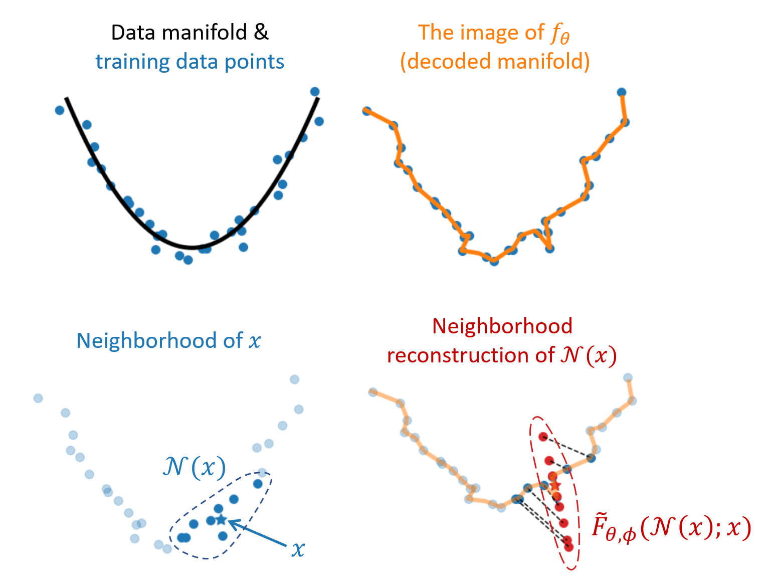
Figure 9: The training data points (blue), the decoded manifold (orange), the neighborhood of $x$ denoted by $\mathcal{N}(x)$, and the neighborhood reconstruction (red). The black dotted lines represent the correspondences between $x^{\prime}\in\mathcal{N}(x)$ and $\tilde{F}_{\theta,\phi}(x^{\prime};x)$.

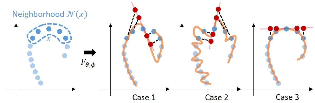
Figure 10: The orange curves represent the learned manifolds, the red points represent the neighborhood reconstruction, and the lengths of the black-dotted lines represent the neighborhood reconstruction loss.

Given that the neighborhood reconstruction of $\mathcal{N}(x)$ reflects the local geometry of the decoded manifold, minimizing a loss function that measures the difference between $\mathcal{N}(x)$ and its image $\tilde{F}_{\theta,\phi}(\mathcal{N}(x);x)$ is one means of training an autoencoder to preserve the local geometry of the original data distribution. With that goal in mind, we formulate a neighborhood reconstruction loss $\mathcal{L}$ as follows:

$$\scriptsize\mathcal{L}(\theta,\phi;\mathcal{D})=\frac{1}{|\mathcal{D}|}\sum_{x\in\mathcal{D}}\frac{1}{|\mathcal{N}(x)|}\sum_{x^{\prime}\in\mathcal{N}(x)}K(x^{\prime},x)\cdot\|x^{\prime}-\tilde{F}_{\theta,\phi}(x^{\prime};x)\|^{2},$$ (19)

where $K(x^{\prime},x)$ is a positive symmetric kernel function that determines the weight for each $x^{\prime}\in\mathcal{N}(x)$. We note that the computations in $\tilde{F}_{\theta,\phi}$ involving derivatives of $f_{\theta}$ can be done by Jacobian-vector and vector-Jacobian products.

Figure 10 illustrates how the neighborhood reconstruction loss can differentiate among the quality of the learned manifolds whose point reconstruction losses are all the same (close to zero): Case 3 has the smallest neighborhood reconstruction loss compared to Case 1 (wrong local geometry) and Case 2 (overfitting).

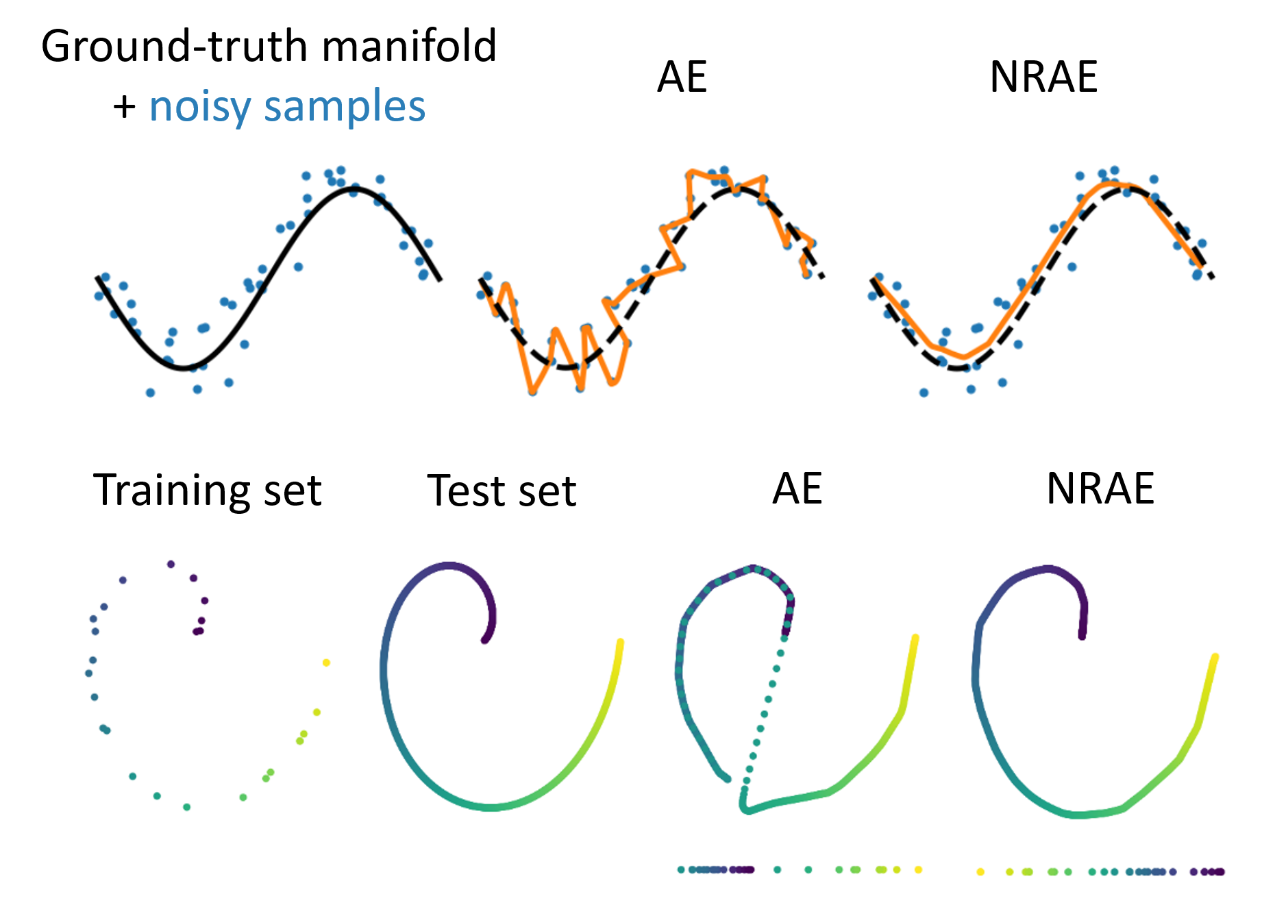
Figure 11: Upper: Given corrupted training data points, NRAE produces more smooth manifold. Lower: Given sparse training data points, NRAE produces a manifold with correct local connectivity (dots below the manifolds represent the one-dimensional latent representations of the training data points).

Figure 11 shows some example results; NRAEs (with quadratic approximations) produce more smooth and accurate manifolds with correct connectivity compared to the vanilla AE.

3.2 Minimum Curvature Autoencoders

In this section, we introduce the extrinsic curvature regularization method for autoencoders  (Lee & Park, 2023), that can resolve the wrong manifold issue to some extent. Recall the local extrinsic curvature measure (10) is

$$\sum_{i,j}\big{(}(J^{T}_{f_{\theta}}HJ_{f_{\theta}})^{-1}\big{)}_{ij}\mathrm{Tr}\big{[}\frac{d\hat{T}}{dz^{i}}\frac{d\hat{T}}{dz^{j}}\big{]},$$

where $\hat{T}=J_{f_{\theta}}(J_{f_{\theta}}^{T}J_{f_{\theta}})^{-1}J_{f_{\theta}}^{T}$. To approximate the trace, consider a set of Gaussian samples $\{w_{k}\sim{\cal N}(0,I_{D\times D})\}_{k=1}^{K}$, and use Hutchinson’s trace estimator:

$$\sum_{i,j}\big{(}(J^{T}_{f_{\theta}}HJ_{f_{\theta}})^{-1}\big{)}_{ij}\frac{1}{K}\sum_{k=1}^{K}\big{[}\frac{d(w_{k}^{T}\hat{T})}{dz^{i}}\frac{d(\hat{T}w_{k})}{dz^{j}}\big{]}.$$

This can be re-written by using the trace as follows:

$$\frac{1}{K}\sum_{k=1}^{K}\mathrm{Tr}\big{[}(J^{T}_{f_{\theta}}HJ_{f_{\theta}})^{-1}(\frac{d(\hat{T}w_{k})}{dz})^{T}\frac{d(\hat{T}w_{k})}{dz}\big{]},$$

where $\frac{d(\hat{T}w_{k})}{dz}$ is a $D\times m$ matrix. We can again use a set of Gaussian samples $\{v_{l}\sim{\cal N}(0,I_{m\times m})\}_{l=1}^{L}$, and use the trace estimator:

$$\frac{1}{K}\sum_{k=1}^{K}\frac{1}{L}\sum_{l=1}^{L}v_{l}^{T}(J^{T}_{f_{\theta}}HJ_{f_{\theta}})^{-1}(\frac{d(\hat{T}w_{k})}{dz})^{T}\frac{d(\hat{T}w_{k})}{dz}v_{l}.$$

In practice, it is sufficient to use one sample in each trace estimation. Because of the matrix inverse computation, we need to compute the full Jacobian, but other computations can be done by Jacobian-vector or vector-Jacobian products.

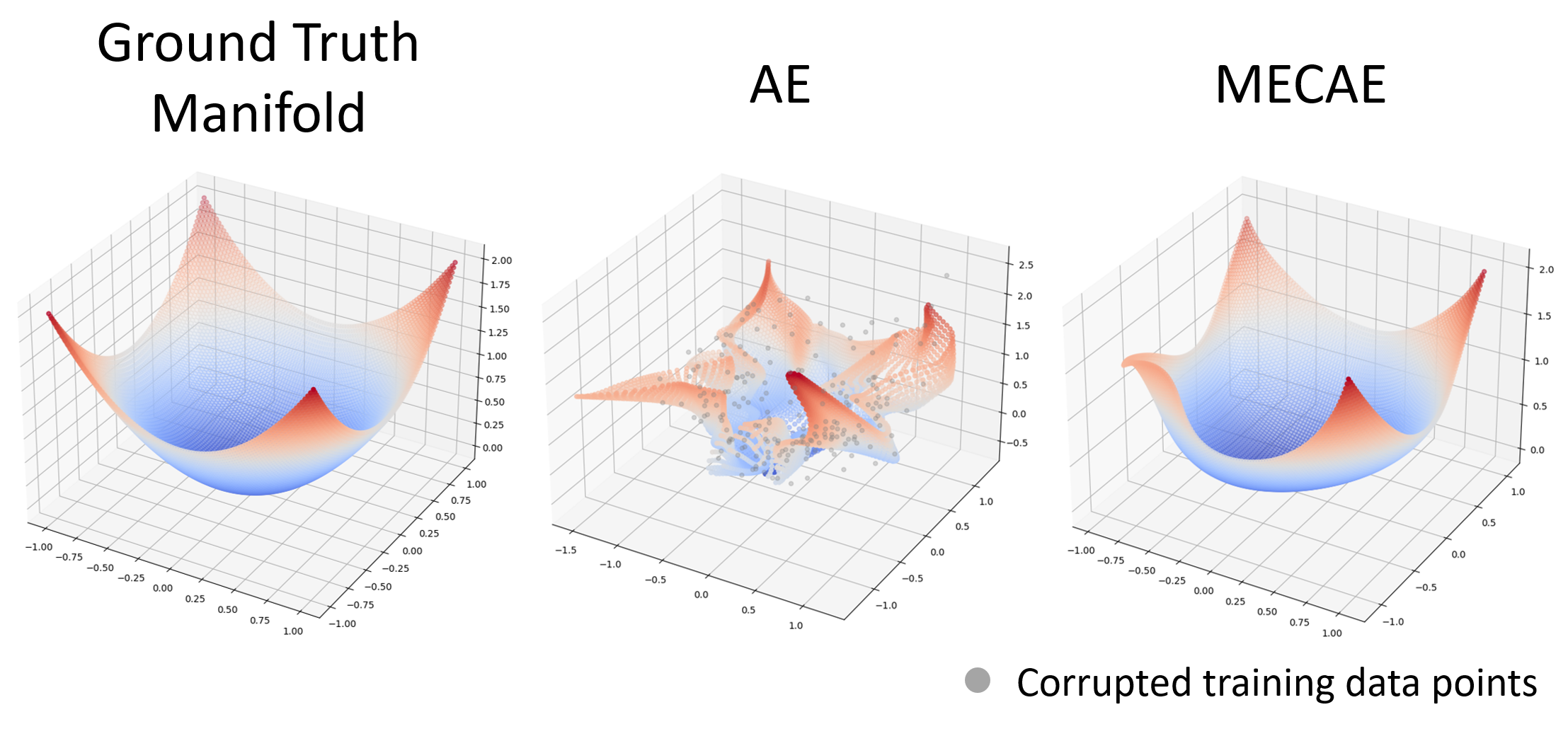
Figure 12: Given corrupted training data points, MECAE – where $H(x)=I_{3\times 3}$ – produces a more smooth and accurate manifold than the AE.

This is a local (approximate) extrinsic curvature measure, and we want to minimize the curvature of the manifold globally. Denoting the local extrinsic curvature measure by $\text{LEC}(z)$, we compute the global curvature measure with respect to some positive measure $\nu$ as follows: $\int_{\mathbb{R}^{m}}\text{LEC}(z)\ d\nu(z).$ In practice, we construct a probability measure $\nu$ by using the encoder function. Let $p_{\phi}(z)$ be a probability density function defined as the push-forward of the data distribution, then it is approximated by an empirical distribution $\frac{1}{|{\cal D}|}\sum_{i}\delta(z-g_{\phi}(x_{i}))$. Using this as $\nu$, the global curvature measure can be approximately computed by $\frac{1}{|{\cal D}|}\sum_{x\in{\cal D}}\text{LEC}(g_{\phi}(x)).$ This is added to the original reconstruction loss function with a suitable weighting parameter $\alpha$:

$$\frac{1}{|{\cal D}|}\sum_{x\in{\cal D}}\big{(}\|F_{\theta,\phi}(x)-x\|^{2}+\alpha\ \text{LEC}(g_{\phi}(x))\big{)},$$ (20)

which is the final objective function for the Minimum Extrinsic Curvature Autoencoder (MECAE); the intrinsic curvature minimization method is also included in (Lee & Park, 2023). Figure 12 shows an example result; MECAE produces a smoother and more accurate manifold.

3.3 Isometrically Regularized Autoencoders

In this section, we explain the isometric regularization method for autoencoders, which attempts to minimize the geometric distortion in the latent space by regularizing the decoder to be a scaled isometry (Lee et al., 2022b). Recall that the relaxed distortion measure (16) is

$$\int_{\mathbb{R}^{m}}\sum_{j=1}^{m}(1-\frac{\lambda_{j}(z)}{\int_{\mathbb{R}^{m}}\sum_{i=1}^{m}\lambda_{i}(z)/m\ d\nu})^{2}\ d\nu,$$

where $\{\lambda_{i}(z)\}=\text{eigenvalues}(J_{f_{\theta}}^{T}(z)H(f(z))J_{f_{\theta}}(z)$). Replacing $\int_{\mathbb{R}^{m}}\cdot\ d\nu$ by $\mathbb{E}_{z\sim P}$ with respect to some probability measure $P$, we can re-write the expression as follows:

$$m^{2}\frac{\mathbb{E}_{z\sim P}[\mathrm{Tr}((J_{f_{\theta}}^{T}HJ_{f_{\theta}})^{2})]}{\mathbb{E}_{z\sim P}[\mathrm{Tr}(J_{f_{\theta}}^{T}HJ_{f_{\theta}})]^{2}}-m.$$

Then, we can use Hutchinson’s trace estimator with Gaussian samples $v,w\sim{\cal N}(0,I_{m\times m})$. Ignoring the constant multiple $m^{2}$ and the shift $-m$, the approximate relaxed distortion measure is

$$\frac{\mathbb{E}_{z\sim P}\big{[}\mathbb{E}_{v}[v^{T}(J_{f_{\theta}}^{T}HJ_{f_{\theta}})^{2}v]\big{]}}{\mathbb{E}_{z\sim P}\big{[}\mathbb{E}_{w}[w^{T}J_{f_{\theta}}^{T}HJ_{f_{\theta}}w]\big{]}^{2}},$$

which can be computed by using the Jacobian-vector and vector-Jacobian products efficiently.

We construct a probability measure $P$ by using the encoder function; $p_{\phi}(z)$ is approximated by an empirical distribution $\frac{1}{|{\cal D}|}\sum_{i}\delta(z-g_{\phi}(x_{i}))$. Then, the relaxed distortion measure can be approximately computed. This is added to the original reconstruction loss function with a suitable weighting parameter $\alpha$:

$$\small\frac{1}{|{\cal D}|}\sum_{x\in{\cal D}}\big{(}\|F_{\theta,\phi}(x)-x\|^{2}+\alpha\ \frac{\mathbb{E}_{v}[v^{T}(J_{f_{\theta}}^{T}HJ_{f_{\theta}})\big{|}_{g_{\phi}(x)}^{2}v]}{\mathbb{E}_{w}[w^{T}(J_{f_{\theta}}^{T}HJ_{f_{\theta}})\big{|}_{g_{\phi}(x)}w]^{2}}\big{)},$$ (21)

where $v,w$ are samples from ${\cal N}(0,I_{m\times m})$. In practice, we use one sample for $v$ and $w$, and let $v=w$ for more efficient computation. This is the final loss function for the Isometrically Regularized Autoencoder (IRAE) (Lee et al., 2022b). Figure 13 shows an example result, where IRAE produces a geometry-preserving latent space while AE produces distorted latent space.

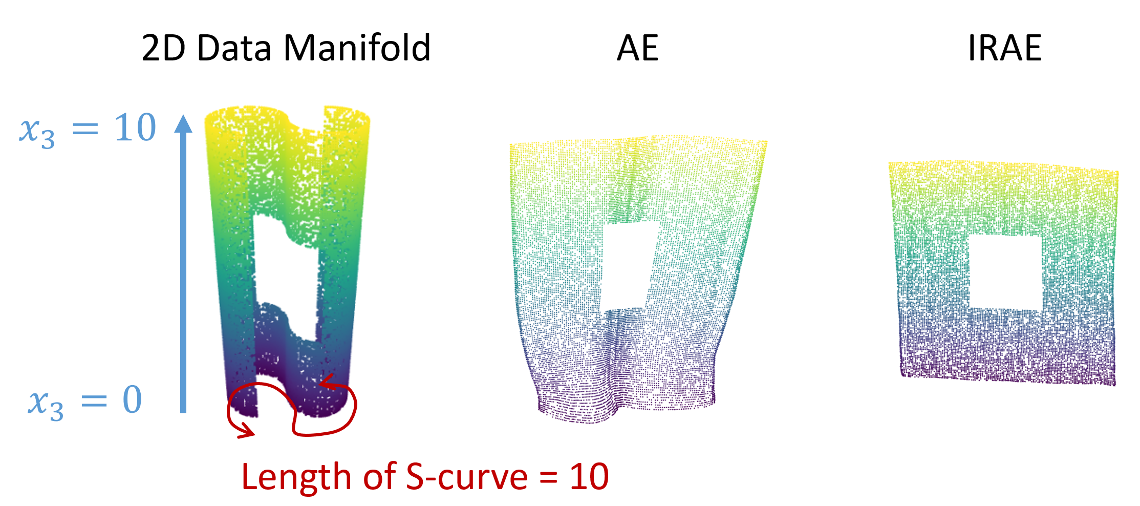
Figure 13: Given a two-dimensional manifold (square-shape manifold with a square hole) in $\mathbb{R}^{3}$, the IRAE – where $H(x)=I_{3\times 3}$ – produces a geometry-preserving latent space, while AE produces distorted latent space.

As discussed in (Lee & Park, 2023), according to Gauss’s Theorema Egregium (i.e., Gauss’s Remarkable Theorem), the Gaussian curvature of a surface is invariant under local isometry. In other words, if two surfaces or manifolds are mapped to each other without distortion, then their Gaussian curvatures or intrinsic curvatures should be preserved. Therefore, if $f$ is a scaled isometry, then since the intrinsic curvature of the Euclidean latent space is everywhere 0, the resulting manifold’s intrinsic curvature must be 0 everywhere as well. As a result, in IRAE, intrinsic curvatures are implicitly minimized as a byproduct of distortion minimization.

In all experiments in (Lee et al., 2022b), the ambient space metric $H$ is assumed to be the identity metric $I_{D\times D}$. There is one specific work that does not use the identity metric in isometric regularization. Lee et al. (2022a) have considered the case where the ambient data space is a point cloud manifold, where each point is a point cloud, and have developed the Info-Riemannian metric for the point cloud manifold based on the theory of information geometry and statistical manifold (Amari, 2016; Amari & Nagaoka, 2000).

4 Conclusions

The geometric understanding, or the manifold learning viewpoint, of the autoencoder framework gives us good insights into what autoencoders actually learn and what problems exist in vanilla autoencoders. In the beginning, we have shown that there are two fundamental issues in the training of autoencoders via reconstruction loss alone: (i) wrong manifold issue and (ii) distorted latent space issue. Then we have introduced three recent works, NRAE (Lee et al., 2021), MCAE (Lee & Park, 2023), and IRAE (Lee et al., 2022b), that address these issues. Commonly, these methods focus on the geometric characteristics of the decoder $f$ by investigating its Jacobian and higher-order derivatives. Considering the memory and computation costs of the derivatives of deep neural networks, practical approximation formulas have been given, relying on the Jacobian-vector and vector-Jacobian products.

In most existing studies, along with the previously mentioned studies, the ambient space metric $H(x)$ was assumed to be identity $I$. The choice of the metric will significantly affect the resulting manifold and representations, and yet, relatively little attention has been given to this problem so far. We believe investigating this aspect further in future research holds promise and is worth exploring.

References

- Amari (2016) Amari, S.-i. Information geometry and its applications, volume 194. Springer, 2016.
- Amari & Nagaoka (2000) Amari, S.-i. and Nagaoka, H. Methods of information geometry, volume 191. American Mathematical Soc., 2000.
- Arvanitidis et al. (2018) Arvanitidis, G., Hansen, L. K., and Hauberg, S. Latent space oddity: on the curvature of deep generative models. In Proceedings of the 6th International Conference on Learning Representations (ICLR), 2018.
- Arvanitidis et al. (2020) Arvanitidis, G., Hauberg, S., and Schölkopf, B. Geometrically enriched latent spaces. arXiv preprint arXiv:2008.00565, 2020.
- Chen et al. (2020) Chen, N., Klushyn, A., Ferroni, F., Bayer, J., and Van Der Smagt, P. Learning flat latent manifolds with vaes. arXiv preprint arXiv:2002.04881, 2020.
- Chen et al. (2021) Chen, X., Wang, C., Lan, X., Zheng, N., and Zeng, W. Neighborhood geometric structure-preserving variational autoencoder for smooth and bounded data sources. IEEE Transactions on Neural Networks and Learning Systems, 2021.
- Do Carmo & Flaherty Francis (1992) Do Carmo, M. P. and Flaherty Francis, J. Riemannian geometry, volume 6. Springer, 1992.
- Duque et al. (2020) Duque, A. F., Morin, S., Wolf, G., and Moon, K. R. Extendable and invertible manifold learning with geometry regularized autoencoders. arXiv preprint arXiv:2007.07142, 2020.
- Fecko (2006) Fecko, M. Differential geometry and Lie groups for physicists. Cambridge university press, 2006.
- Higgins et al. (2016) Higgins, I., Matthey, L., Pal, A., Burgess, C., Glorot, X., Botvinick, M., Mohamed, S., and Lerchner, A. beta-vae: Learning basic visual concepts with a constrained variational framework. 2016.
- Hutchinson (1989) Hutchinson, M. F. A stochastic estimator of the trace of the influence matrix for laplacian smoothing splines. Communications in Statistics-Simulation and Computation, 18(3):1059–1076, 1989.
- Jang (2019) Jang, C. Riemannian Distortion Measures for Non-Euclidean Data. PhD thesis, Seoul National University Graduate School, 2019.
- Jang et al. (2020) Jang, C., Noh, Y.-K., and Park, F. C. A riemannian geometric framework for manifold learning of non-euclidean data. Advances in Data Analysis and Classification, pp. 1–27, 2020.
- Jang et al. (2022) Jang, C., Lee, Y., Noh, Y.-K., and Park, F. C. Geometrically regularized autoencoders for non-euclidean data. In The Eleventh International Conference on Learning Representations, 2022.
- Kingma & Welling (2013) Kingma, D. P. and Welling, M. Auto-encoding variational bayes. arXiv preprint arXiv:1312.6114, 2013.
- Kramer (1991) Kramer, M. A. Nonlinear principal component analysis using autoassociative neural networks. AIChE journal, 37(2):233–243, 1991.
- LeCun et al. (2015) LeCun, Y., Bengio, Y., and Hinton, G. Deep learning. nature, 521(7553):436–444, 2015.
- Lee & Park (2023) Lee, Y. and Park, F. C. On explicit curvature regularization in deep generative models. In 2nd Annual Workshop on Topology, Algebra, and Geometry in Machine Learning (TAG-ML), 2023.
- Lee et al. (2021) Lee, Y., Kwon, H., and Park, F. Neighborhood reconstructing autoencoders. Advances in Neural Information Processing Systems, 34, 2021.
- Lee et al. (2022a) Lee, Y., Kim, S., Choi, J., and Park, F. A statistical manifold framework for point cloud data. In International Conference on Machine Learning, pp. 12378–12402. PMLR, 2022a.
- Lee et al. (2022b) Lee, Y., Yoon, S., Son, M., and Park, F. C. Regularized autoencoders for isometric representation learning. In International Conference on Learning Representations, 2022b. URL https://openreview.net/forum?id=mQxt8l7JL04.
- Makhzani et al. (2015) Makhzani, A., Shlens, J., Jaitly, N., Goodfellow, I., and Frey, B. Adversarial autoencoders. arXiv preprint arXiv:1511.05644, 2015.
- Rifai et al. (2011) Rifai, S., Vincent, P., Muller, X., Glorot, X., and Bengio, Y. Contractive auto-encoders: Explicit invariance during feature extraction. In Icml, 2011.
- Shao et al. (2018) Shao, H., Kumar, A., and Thomas Fletcher, P. The riemannian geometry of deep generative models. In Proceedings of the IEEE Conference on Computer Vision and Pattern Recognition Workshops, pp. 315–323, 2018.
- Tolstikhin et al. (2017) Tolstikhin, I., Bousquet, O., Gelly, S., and Schoelkopf, B. Wasserstein auto-encoders. arXiv preprint arXiv:1711.01558, 2017.
- Vincent et al. (2010) Vincent, P., Larochelle, H., Lajoie, I., Bengio, Y., Manzagol, P.-A., and Bottou, L. Stacked denoising autoencoders: Learning useful representations in a deep network with a local denoising criterion. Journal of machine learning research, 11(12), 2010.