Quantum Hall effect in topological Dirac semimetals modulated by the Lifshitz transition of the Fermi arc surface states

Abstract

We investigate the magnetotransport of topological Dirac semimetals (DSMs) by taking into account the Lifshitz transition of the Fermi arc surface states. We demonstrate that a bulk momentum-dependent gap term, which is usually neglected in study of the bulk energy-band topology, can cause the Lifshitz transition by developing an additional Dirac cone for the surface to prevent the Fermi arcs from connecting the bulk Dirac points. As a result, the Weyl orbits can be turned off by the surface Dirac cone without destroying the bulk Dirac points. In response to the surface Lifshitz transition, the Weyl-orbit mechanism for the 3D quantum Hall effect (QHE) in topological DSMs will break down. The resulting quantized Hall plateaus can be thickness-dependent, similar to the Weyl-orbit mechanism, but their widths and quantized values become irregular. Accordingly, we propose that apart from the bulk Weyl nodes and Fermi arcs, the surface Lifshitz transition is also crucial for realizing stable Weyl orbits and 3D QHE in real materials.

I introduction

Topological semimetals are novel quantum states of matter, in which the conduction and valence bands cross near the Fermi level at certain discrete momentum points or linesArmitage et al. (2018); Neupane et al. (2014); Wang et al. (2013, 2012); Liu et al. (2014); Yang and Nagaosa (2014); Wan et al. (2011); Zhang et al. (2016, 2017); Wang et al. (2017). The gap-closing points or lines are protected either by crystalline symmetry or topological invariantsGorbar et al. (2015); Kargarian et al. (2016). A topological Dirac semimetal (DSM) hosts paired gap-closing points, referred to as the Dirac points, which are stabilized by the time-reversal, spatial-inversion and crystalline symmetries. By breaking the time-reversal or spatial-inversion symmetry, a single Dirac point can split into a pair of Weyl nodes of opposite chiralitiesNielsen and Ninomiya (1983); Volovik (2003), leading to the topological transition from a Dirac to a Weyl semimetalRaza et al. (2019); Zyuzin et al. (2012); Goswami and Tewari (2013); Han et al. (2018); Deng et al. (2017); Chen et al. (2019). Accompanied with the bulk topological transition, topological states which are protected by the quantized Chern flux will emerge in the surface to connect the split Weyl nodes, known as the Fermi-arc surface statesWan et al. (2011).

In topological DSMs, such as A₃Bi (A = Na,K,Rb)Wang et al. (2012); Liu et al. (2014) and Cd₂As₃Wang et al. (2013); Neupane et al. (2014), the Weyl nodes at the same Dirac point, belonging to different irreducible representations, cannot be coupled and have to seek for a partner from the other Dirac point. As a consequence, the two Dirac points including two pairs of Weyl nodes are connected by two spin-polarized Fermi arcsWang et al. (2012, 2013); Liu et al. (2014); Yang and Nagaosa (2014); Wan et al. (2011). The Fermi-arc surface states are the most distinctive observable spectroscopic feature of topological semimetals. However, their observation is sometime limited by spectroscopic resolutions. There have been searching for alternative smoking-gun features of topological semimetals, such as by means of transport phenomenaAli et al. (2014); Shekhar et al. (2015); Parameswaran et al. (2014). Many interesting transport properties have been revealed in topological semimetals, for example, chiral anomaly induced negative magnetoresistanceXiong et al. (2015); Li et al. (2015); Deng et al. (2019a, b), Weyl-orbit related quantum oscillationsPotter et al. (2014); Moll et al. (2016), Berry’s phase $\pi$ related Aharonov-Bohm effectLin et al. (2017); Wang et al. (2016), bulk-surface interference induced Fano effectWang et al. (2018), topological pumping effectDeng et al. (2022), etc.

Recently, 3D quantum Hall effect (QHE) because of the Fermi arcs was proposed in Weyl semimetalsWang et al. (2017) and has led to an explosion of theoreticalLi et al. (2020); Ma et al. (2021); Geng et al. (2021); Chang et al. (2021); Chang and Sheng (2021); Lu (2018); Li et al. (2021); Qin et al. (2020); Gooth et al. (2023); Wang and Cai (2023); Du et al. (2021) and experimentalUchida et al. (2017); Schumann et al. (2018); Zhang et al. (2019); Tang et al. (2019); Lin et al. (2019) activities in the field of condensed matter physics. In a Weyl semimetal slab, the Weyl orbit which consists of Fermi arcs from opposite surfaces can support the electron cyclotron orbit for the QHE, making the 3D QHE available. The 3D QHE has been observed experimentally in topological DSMsUchida et al. (2017); Schumann et al. (2018); Zhang et al. (2019); Tang et al. (2019); Lin et al. (2019) and the one from the Weyl-orbit mechanism is demonstrated to be thickness-dependent Zhang et al. (2019). However, for the topological DSMs, a single surface with two Fermi arcs can also support a complete Fermi loop required by the QHE, which can compete with the Weyl-orbit mechanism. The same-surface Fermi loop is not stable and can be deformed by bulk perturbationsKargarian et al. (2016). In real materials, the bulk perturbations are inevitable.

As we will show, when a bulk momentum-dependent gap term is included, Lifshitz transition can happen for the Fermi arc surface states, in which the double Fermi arcs on the DSM surface can be continuously deformed into a closed Fermi loop and separate from the bulk Dirac points. The Lifshitz transition involves a change of the Fermi surface topology that is not connected with a change in the symmetry of the latticeLifshitz (1960); Okada et al. (2013); Zeljkovic et al. (2014); Wu et al. (2015); Ding et al. (2021). Therefore, the Lifshitz transition can take place without destroying the topology of the bulk energy band. A natural question in this regard is how the deformation of the Fermi arcs influences the 3D QHE of topological DSMs, especially when the Fermi arcs, as key ingredients for the Weyl orbits, breaks free from the bulk Dirac points.

In this paper, we investigate the QHE in topological DSMs by taking into account the surface Lifshitz transition, which can be modulated by a bulk momentum-dependent gap term. It is demonstrated that while the bulk Dirac points are robust against the momentum-dependent gap term, the surface can develop an additional 2D Dirac cone, which deforms the surface Fermi arcs from a curve to some discrete points and further to a Fermi loop coexisting with the bulk Dirac points. During this process, the bulk topological properties do not change, but the Weyl orbits can be turned off. The joint effect of the Weyl orbits and surface Lifshitz transition can make the QHE quite complicated. We find that when the Weyl orbits are broken by the surface Dirac cone, the bulk and surface states can form the Landau levels (LLs) and contribute the QHE, independently. The resulting Hall plateaus are sensitive to the thickness of the sample, but their widths and quantized values are irregularly distributed. The rest of this paper is organized as follows. In Sec. II, we introduce the model Hamiltonian and bulk spectrum. The Lifshitz transition of the Fermi arcs and the LLs are analyzed in Sec. III and Sec. IV, respectively. The QHE is studied in Sec. V and the last section contains a short summary.

II Hamiltonian and bulk spectrum

We begin with a low-energy effective Hamiltonian for the topological DSMs

$$\mathcal{H}(\bm{k})=\varepsilon_{\bm{k}}+\lambda(k_{x}\sigma_{z}\tau_{x}-k_{y}\tau_{y})+m_{\bm{k}}\tau_{z}+\Lambda(\bm{k})$$ (1)

with $m_{\bm{k}}=m_{0}-m_{1}k_{z}^{2}-m_{2}k_{\parallel}^{2}$ and $\varepsilon_{\bm{k}}=c_{0}+c_{1}k_{z}^{2}+c_{2}k_{\parallel}^{2}$, where $k_{\parallel}=\sqrt{k_{x}^{2}+k_{y}^{2}}$ and $\sigma_{x,y,z}$ ($\tau_{x,y,z}$) is the Pauli matrix acting on the spin (orbital parity) degree of freedom. This model has been widely-adopted to capture the topological properties of topological DSMs Cd₃As₂Wang et al. (2013) and A₃Bi (A = Na, K, Rb)Wang et al. (2012). In the absence of $\Lambda(\bm{k})$, $\left[\sigma_{z},\mathcal{H}(\bm{k})\right]=0$ and the topological DSMs characterized by Hamiltonian (1) can be viewed as two superposed copies of a Weyl semimetal with two Weyl nodes, which possesses two sets of surface Fermi arcs in the surface Brillouin zone, as illustrated by Figs. 1(a)-(b) and (e)-(f). $\Lambda(\bm{k})$ mixes the eigenstates of opposite spins away from the Dirac points and plays the role of a momentum-dependent gap term, whose form is determined by the crystal symmetries.

Specifically, for a DSM with fourfold rotational symmetry, such as Cd₃As₂, the momentum-dependent gap term can take the form $\Lambda(\bm{k})=\alpha k_{z}\left(k_{+}^{2}\sigma_{-}+k_{-}^{2}\sigma_{+}\right)\tau_{x}/2$ with $k_{\pm}=k_{x}\pm ik_{y}$ and $\sigma_{\pm}=\sigma_{x}\pm i\sigma_{y}$. Diagonalizing Hamiltonian (1) yields the continuum bulk spectrum

$$E_{\pm}(\bm{k})=\varepsilon_{\bm{k}}\pm\sqrt{\lambda^{2}k_{\parallel}^{2}+m_{\bm{k}}^{2}+\alpha^{2}k_{\parallel}^{4}k_{z}^{2}},$$ (2)

from which we can determine the energy location $E_{D}=c_{0}+c_{1}k_{w}^{2}$ and momentum locations $\bm{K}_{\pm}=(0,0,\pm k_{w})$ of the bulk Dirac points with $k_{w}=\sqrt{m_{0}/m_{1}}$. As $\varepsilon_{\bm{k}}$ possesses the symmetries of $m_{\bm{k}}$, it does not qualitatively change the Dirac spectrum in the bulk, but introduces an asymmetry between the positive (electrons) and negative (holes) energy branches and, consequently, breaks the particle-hole symmetry. The electron-hole asymmetry will curve the Fermi arcs, which was demonstrated to be crucial for the LLs around the Weyl nodesWang et al. (2017). While $\Lambda(\bm{k})$ can profoundly change the spectrum of quasiparticles for sufficiently large $k_{\parallel}$, it preserves all the symmetries of the crystal structure and vanishes at the Dirac points. Therefore, the bulk Dirac points are robust against $\Lambda(\bm{k})$, as seen from Eq. (2) that both the momentum and energy locations of the Dirac points are regardless of $\alpha$. For this reason, $\Lambda(\bm{k})$ was usually treated as a bulk perturbation, which does not destroy the bulk topology.

Figure 1: (a)-(d) The dispersion (red) by diagonalizing Hamiltonian (12) for (a) $\alpha=0$, $c_{1}=c_{2}=0$, (b) $\alpha=0$, $c_{1}=3c_{2}=0.15$, (c) $\alpha=0.5$, $c_{1}=c_{2}=0$, and (d) $\alpha=0.5$, $c_{1}=3c_{2}=0.15$, with $k_{x}=0$ and $E_{D}=0$ denoted by the blue-dashed lines. The green dotted curves are determined from Eq. (9), self-consistently. (e)-(h) The $\bm{k}$-resolved DOSs corresponding to (a)-(d) at $E_{F}=E_{D}$. The rest parameters are set as $\lambda=0.5$, $k_{w}=\pi/4$, $m_{0}=\pi^{2}/32$, $m_{2}=0.5$ and $N_{y}=50$.

For the states close to the bulk Dirac points, the quasiparticles can be described by linearizing Hamiltonian (1) around $\bm{K}_{\pm}$, such that $\Lambda(\bm{k})$ can be neglected. However, for a topological DSM slab, the Fermi arcs, which connect the bulk Dirac points separated far away in momentum space, can extend to large $\bm{k}$ where the spectrum can be dramatically modified by the momentum-dependent gap term. In the following, we elucidate that, in response to the momentum-dependent gap term, the surface states of topological DSMs will experience a Lifshitz transition, during which process, the Fermi arcs can exist without connecting the bulk Dirac points.

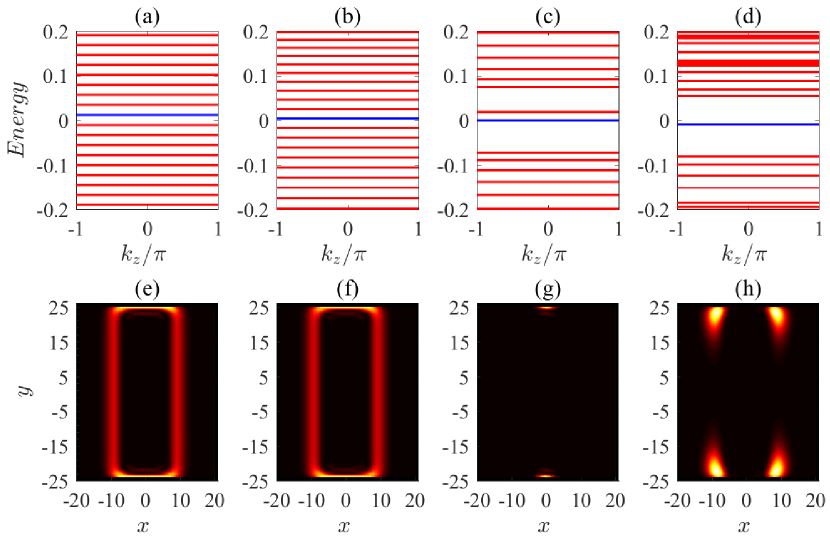
Figure 2: The LLs for (a) $\alpha=0$, $c_{1}=c_{2}=0$, (b) $\alpha=0$, $c_{1}=3c_{2}=0.15$, (c) $\alpha=0.5$, $c_{1}=c_{2}=0$, and (d) $\alpha=0.5$, $c_{1}=3c_{2}=0.15$. (e)-(h) The probability density $|\psi_{k_{z},\mu}|^{2}$ for the blue LLs in (a)-(d), in which $\psi_{k_{z},\mu}$ is the $\mu$-th LL’s wavefunction. Here, we set $2\pi\ell_{B}^{2}=N_{x}$, $k_{z}=\pi$, $k_{w}=\pi/2$, $N_{x}=40$ and other parameters the same as Fig. 1.

III Lifshitz transition of the Fermi arcs

To better understand how the Fermi arc surface states evolve with the momentum-dependent gap term, we consider a topological DSM slab with open boundaries at $y=\pm L/2$ and derive the surface states for the $x$-$z$ plane. For such a finite-size system, $k_{y}$ in Eq. (1) is not longer a good quantum number and should be replaced with the operator $-i\partial_{y}$. In the spirit of the perturbation theory, we construct an unperturbed surface basis by the surface wavefunctions without $\Lambda(\bm{k})$ and the effective Hamiltonian for the surface states can be obtained by projecting Eq. (1) onto the unperturbed surface basis. For the convenience of discussion, we assume $m_{2}>|c_{2}|$ and select $E_{D}$ as potential energy zero, i.e., $c_{0}=-c_{1}k_{w}$.

By setting $\alpha=0$ and solving the differential equation $\mathcal{H}$$(k_{x},-i\partial_{y},k_{z})\Psi_{k_{x},k_{z}}(y)=E\Psi_{k_{x},k_{z}}(y)$ with the open boundary conditions $\Psi_{k_{x},k_{z}}(\pm L/2)=0$, we can evaluate the unperturbed surface wavefunctions as $\Psi_{k_{x},k_{z}}^{\beta,s}(y)=\left(\frac{1+s}{2},\frac{1-s}{2}\right)^{T}\otimes\Psi_{\beta}(y)$, which are spin-resolved, with $s=\pm 1$ being the eigenvalue of $\sigma_{z}$ and

$$\Psi_{\beta}(y)=\left(\begin{array}[c]{c}\beta\cos\frac{\vartheta}{2}\\ -\sin\frac{\vartheta}{2}\end{array}\right)\frac{e^{\kappa_{-}(\beta y-\frac{L}{2})}-e^{\kappa_{+}(\beta y-\frac{L}{2})}}{\sqrt{N_{\beta}}}.$$ (3)

Here, $\beta=\pm$ corresponds to the surface at $y=\pm L/2$, $N_{\beta}=\int_{-\frac{L}{2}}^{\frac{L}{2}}|e^{\kappa_{-}(\beta y-\frac{L}{2})}-e^{\kappa_{+}(\beta y-\frac{L}{2})}|^{2}dy$ is the normalization coefficient and

$$\vartheta=\tan^{-1}\left[\frac{2\lambda\left(m_{2}-c_{2}\right)\left(\kappa_{+}+\kappa_{-}\right)}{\lambda^{2}-\left(m_{2}-c_{2}\right)^{2}\left(\kappa_{+}+\kappa_{-}\right)^{2}}\right],$$ (4)

in which $\kappa_{\pm}$ is a solution to $E_{\pm}(k_{x},-i\kappa,k_{z})=E$, reading as

$$\kappa_{\pm}=\sqrt{k_{x}^{2}+\frac{\zeta_{\lambda}\pm\left(\zeta_{\lambda}^{2}-\zeta_{+}\zeta_{-}\right)^{1/2}}{m_{2}^{2}-c_{2}^{2}}}$$ (5)

with $\zeta_{\lambda}=\frac{\lambda^{2}-\zeta_{+}+\zeta_{-}}{2}$ and

$$\zeta_{\pm}=\left(m_{2}\pm c_{2}\right)\left[\left(m_{1}\mp c_{1}\right)\left(k_{w}^{2}-k_{z}^{2}\right)\mp E\right].$$ (6)

The surface states are confined within the region defined by $\operatorname{Re}(\kappa_{\pm})>0$. Subsequently, by performing the projection operation

$$\mathcal{H}_{\mathrm{surf}}^{\beta,ss^{\prime}}=\langle\Psi_{k_{x},k_{z}}^{\beta,s}(y)|\mathcal{H}(k_{x},-i\partial_{y},k_{z})|\Psi_{k_{x},k_{z}}^{\beta,s^{\prime}}(y)\rangle,$$ (7)

we can obtain the effective surface Hamiltonian

$$\mathcal{H}_{\mathrm{surf}}^{\beta}\left(k_{x},k_{z}\right)=\tilde{\varepsilon}_{\bm{k}}-\beta\sin\vartheta\left(\lambda k_{x}\sigma_{z}+\tilde{\alpha}k_{z}\sigma_{x}\right),$$ (8)

where $\tilde{\alpha}=\alpha\left(k_{x}^{2}-\kappa_{+}\kappa_{-}\right)$, $\tilde{\varepsilon}_{\bm{k}}=\tilde{c}_{1}\left(k_{z}^{2}-k_{w}^{2}\right)+\tilde{c}_{2}\left(k_{x}^{2}+\kappa_{+}\kappa_{-}\right)$ and $\tilde{c}_{l}=c_{l}-m_{l}\cos\vartheta$ with $l=1,2$.

As shown by Eq. (8), the surface Hamiltonian exhibits a 2D Dirac structure with spin-momentum locking, which resembles the surface states for 3D topological insulators. However, as different from the 3D topological insulators, the bulk spectrum here is also gapless, namely, the surface Dirac point can coexist with the bulk Dirac points. By diagonalizing Eq. (8), we can arrive at

$$E_{\eta}^{\beta}\left(k_{x},k_{z}\right)=\tilde{\varepsilon}_{\bm{k}}-\eta\beta\sin\vartheta\sqrt{\lambda^{2}k_{x}^{2}+\tilde{\alpha}^{2}k_{z}^{2}},$$ (9)

where $\eta=\pm 1$ labels the conduction/valence band. It should be noted that, because $\kappa_{\pm}$ is energy dependent, Eq. (9) is only a formal solution for the surface spectrum. The exact surface dispersion involves a self-consistent calculation of Eq. (9) via replacing $E\rightarrow E_{\eta}^{\beta}\left(k_{x},k_{z}\right)$ in Eq. (6). The numerical results of the surface dispersion are presented by the green dotted curves in Figs. 1(a)-(d).

In order to show the bulk states and surface Fermi arcs, simultaneously, we evaluate the $\bm{k}$-resolved density of states (DOSs) for a given energy $E$ through

$$\rho\left(E,k_{x},k_{z}\right)=-\frac{1}{\pi}\operatorname{Im}\mathrm{Tr}\left(\frac{1}{E+i0^{+}-H}\right),$$ (10)

in which $H=\sum_{\bm{k}}c_{\bm{k}}^{{\dagger}}\mathcal{H}_{\bm{k}}^{\mathrm{tb}}c_{\bm{k}}$ is the tight-binding Hamiltonian corresponding to Eq. (1). Here, $c_{\bm{k}}^{{\dagger}}$ ($c_{\bm{k}}$) is the fermion creation (annihilation) operator and

$$\mathcal{H}_{\bm{k}}^{\mathrm{tb}} =M_{\bm{k}}+\lambda\left(\sin k_{x}\sigma_{z}\tau_{x}-\sin k_{y}\tau_{y}\right)-2\alpha\sin k_{z}$$

$$\times\left[\left(\cos k_{x}-\cos k_{y}\right)\sigma_{x}-\sin k_{x}\sin k_{y}\sigma_{y}\right]\tau_{x}$$ (11)

is the single-particle Hamiltonian obtained from Eq. (1) via the transforms $k_{a}\rightarrow\sin k_{a}$ and $k_{a}^{2}\rightarrow 2-2\cos k_{a}$, with $a=x,y,z$, $M_{\bm{k}}=f_{1}\left(\cos k_{z}-\cos k_{w}\right)+f_{2}\left(\cos k_{x}+\cos k_{y}-2\right)$ and $f_{l}=2(m_{l}\tau_{z}-c_{l})$. By performing the Fourier transform $c_{\bm{k}}\rightarrow\sum_{n}c_{n}e^{-ik_{y}y_{n}}$, we can discretize the tight-binding Hamiltonian as

$$H=\sum_{n}c_{n}^{{\dagger}}h_{0}c_{n}+\sum_{n}\left(c_{n}^{{\dagger}}h_{y}c_{n+1}+h.c.\right),$$ (12)

where the hopping matrices are given by

$$h_{0} =f_{0}+f_{1}\cos k_{z}+f_{2}\cos k_{x}+f_{x}\sin k_{x}$$

$$-\alpha\sigma_{x}\tau_{x}\left[\sin\left(k_{z}+k_{x}\right)+\sin\left(k_{z}-k_{x}\right)\right]$$ (13)

$$h_{y} =\frac{f_{2}+if_{y}}{2}+\alpha\sigma_{x}\tau_{x}\sin k_{z}$$

$$+i\alpha\sigma_{y}\tau_{x}\frac{\cos\left(k_{z}+k_{x}\right)-\cos\left(k_{z}-k_{x}\right)}{2}$$ (14)

with $f_{0}=-2f_{2}-f_{1}\cos k_{w}$ and $f_{x(y)}=\lambda\sigma_{z(0)}\tau_{x(y)}$.

In Fig. 1, we plot the numerical spectrum and $\bm{k}$-resolved DOSs for Eq. (12). As shown by the green dotted curves in Figs. 1(a)-(d), the self-consistent calculation of Eq. (9) coincides with the results by the numerical diagonalization of Eq. (12). As illustrated by Figs. 1(a) and (e), the surface spectrums without $\varepsilon_{\bm{k}}$ and $\Lambda(\bm{k})$ are $k_{z}$-independent and cross at $E_{D}$ with a quadruply degenerate line connecting the two Dirac points. The flat Fermi line can be easily modified by perturbations. This explains why the particle-hole symmetry and the momentum-dependent gap term are important to the surface states. A nonzero $\varepsilon_{\bm{k}}$ can not gap the surface spectrum, but will bend the Fermi lines to a parabola, as shown by Fig. 1(b). As a result, the Fermi arcs with opposite spin, due to the spin-dependent term in Eq. (8), will curve in opposite direction at the Fermi level, forming a closed loop with a discontinuous kink at the Dirac points, as indicated by Fig. 1(f).

By contrast, when the momentum-dependent gap term is included, the Fermi lines with opposite spin, because of the noncommutation between $\sigma_{z}$ and $\mathcal{H}_{\mathrm{surf}}^{\beta}\left(k_{x},k_{z}\right)$, will repel each other and so remove the spin degeneracy. Since $\Lambda(\bm{k})=0$ for $k_{\parallel}=0$ or $k_{z}=0$, the surface spectrums keep crossing at $\bm{k}=0,\bm{K}_{\pm}$, as shown by Fig. 1(c). Therefore, a 2D Dirac point develops on each surface, which coexists with the bulk Dirac points. The surface Dirac points, similar to the bulk Dirac points, are robust against $\Lambda(\bm{k})$, but, differently, the energy location of the surface Dirac points can be modulated by the particle-hole asymmetry. In the presence of particle-hole symmetry, i.e., $\varepsilon_{\bm{k}}=0$, the energy location of the surface Dirac points is identical to the bulk Dirac points, such that at $E_{F}=E_{D}$, the Fermi line in Fig. 1(e) deforms into three Fermi points in Fig. 1(g). When the particle-hole symmetry is broken by a finite $\varepsilon_{\bm{k}}$, the surface Dirac points will shift away from $E_{D}$, after that the surface Fermi point around $\bm{k}=0$ turns to a Fermi loop, as demonstrated by Fig. 1(h), which prevents the Fermi arcs from connecting the bulk Dirac points.

Consequently, although the surface spectrums remain intersecting with the bulk Dirac points, the surface states will experience a Lifshitz transition with the Fermi arcs changing from a curve to some discrete gap-closing points and further to a Fermi loop coexisting with the bulk Dirac points, during which process the Weyl orbits can be turned off without destroying the topological properties of the bulk energy band.

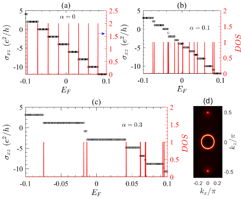
Figure 3: The Hall conductivity (left axis) and DOS (right axis) for a given $k_{z}$ with (a) $\alpha=0$, (b) $\alpha=0.1$ and (c) $\alpha=0.3$. (d) The Fermi surface for $E_{F}=0$ and $\alpha=0.3$ in the absence of magnetic field. The parameters are the same as Fig. 2.

IV LLs and probability density distribution

Upon application of an external magnetic field, a Peierls phase should be added to the hopping matrices as electrons jump from position $\bm{r}_{n}$ to $\bm{r}_{m}$, i.e., $t_{mn}\rightarrow t_{mn}e^{-i\varphi_{mn}}$ with $\varphi_{mn}=\frac{2\pi}{\Phi_{0}}\int_{\bm{r}_{m}}^{\bm{r}_{n}}\bm{A}\cdot d\bm{l}$ and $\Phi_{0}=h/e$ being the unit flux quantum. For the magnetic field is applied in the $y$ direction, we can choose the Landau gauge $\bm{A}=(0,0,-Bx)$. To include the magnetic field, we further discretize Eq. (12) in direction $x$ as

$$H =\sum_{mn}c_{m,n}^{{\dagger}}(T_{m}c_{m,n}+T_{m,x}c_{m+1,n}+T_{m,y}c_{m,n+1}$$

$$+T_{m,\alpha}c_{m+1,n-1}-T_{m,\alpha}c_{m+1,n+1})+h.c.,$$ (15)

in which the Fourier transform $c_{n}\rightarrow\sum_{m}c_{m,n}e^{-ik_{x}x_{m}}$ has been adopted and the hopping matrices are

$$T_{m} =\frac{f_{0}+f_{1}\cos\left(k_{z}-m/\ell_{B}^{2}\right)}{2},$$ (16)

$$T_{m,\alpha} =\frac{\alpha}{2}\sigma_{y}\tau_{x}\sin\left(k_{z}-\frac{m+1/2}{\ell_{B}^{2}}\right),$$ (17)

$$T_{m,y} =\frac{f_{2}+if_{y}}{2}+\alpha\sigma_{x}\tau_{x}\sin\left(k_{z}-m/\ell_{B}^{2}\right),$$ (18)

$$T_{m,x} =\frac{f_{2}-if_{x}}{2}-\alpha\sigma_{y}\tau_{x}\sin\left(k_{z}-\frac{m+1/2}{\ell_{B}^{2}}\right),$$ (19)

with $\ell_{B}=\sqrt{\hbar/\left(eB\right)}$ being the magnetic length.

After introducing the magnetic field, we continue to demonstrate the relation between Eq. (11) and Eq. (15). By the inverse Fourier transform on Eq. (15), we can arrive at

$$\mathcal{\tilde{H}}_{\bm{k}} =f_{1}\left(\cos\kappa_{z}-\cos k_{w}\right)+f_{2}\left(\cos k_{x}+\cos k_{y}-2\right)$$

$$+\lambda\left(\sin k_{x}\tau_{x}\sigma_{z}-\sin k_{y}\tau_{y}\right)-\alpha\tau_{x}[(\frac{\sin\kappa_{z}^{+}-\sin\kappa_{z}^{-}}{2}$$

$$-\cos k_{y}\sin\kappa_{z})\sigma_{x}-\sin k_{y}\frac{\cos\kappa_{z}^{+}-\cos\kappa_{z}^{-}}{2}\sigma_{y}]$$ (20)

with $\kappa_{z}=k_{z}-x/\ell_{B}^{2}$ and $\kappa_{z}^{\pm}=\pm\kappa_{z}+k_{x}$. Here, we have used the Baker-Campbell-Hausdorff formula, i.e., $e^{\hat{A}+\hat{B}}=e^{\hat{A}}e^{\hat{B}}e^{-\frac{1}{2}[\hat{A},\hat{B}]}$. It is clear that $\mathcal{\tilde{H}}_{\bm{k}}=\mathcal{H}_{\bm{k}\rightarrow\bm{k}+e\bm{A}/\hbar}^{\mathrm{tb}}$ follows the Peierls substitution. However, for $\alpha\neq 0$, one should be very careful when using the direct Peierls substitution, because of the cross momentum term in $\Lambda(\bm{k})$. For example, as we transform Eq. (20) to the lattice form for numerical calculation, there will emerge an additional phase $\ell_{B}^{-2}/2$, such as in Eqs. (17) and (19). The underlying physics for the additional phase is that after the Peierls substitution, the different momentum components can be noncommutative, e.g., $[k_{x},\kappa_{z}]=$ $i\ell_{B}^{-2}$, and the Baker-Campbell-Hausdorff formula must be adopted. For instance, when transforming Eq. (12) to Eq. (15), one should express the trigonometric functions in the exponential form and then introduce the Peierls phase via the transforms $e^{ik_{z}}\rightarrow e^{i\kappa_{z}}$ and $e^{i\left(k_{x}\pm k_{z}\right)}\rightarrow e^{i\kappa_{z}^{\pm}}=e^{\pm i\left(\kappa_{z}-\ell_{B}^{-2}/2\right)}e^{ik_{x}}$.

By diagonalizing Hamiltonian (15) numerically, we can obtain the LLs and spatial distribution of the electron probability density, as displayed in Fig. 2. Through the spatial distribution of the probability density, we can tell easily whether or not the LLs are formed by the Weyl orbits. From Figs. 2(a) and (e), we see that the LLs can be formed from the Weyl-orbit mechanism, even when there is no curvature in the Fermi arcs. In the Weyl-orbit mechanism, the surface fermions, driven by the magnetic field, will move along the Fermi arcs from one Dirac valley to the other and tunnel to the opposite surface at the Dirac points via the bulk states. Therefore, the probability density exhibits a closed loop with two bright stripes crossing the bulk and connecting the surface states, as seen from Fig. 2(e). The width of the bright stripes $\sim 2\ell_{B}$ relates to the cyclotron radius of the bulk Dirac fermions and the distance between the stripes encodes the momentum distance between the Dirac points. The cyclotron center $x_{c}=\ell_{B}^{2}k_{z}$ of the fermions in different Dirac valleys differs by $\Delta x_{c}=2\ell_{B}^{2}k_{w}$, which is exactly the distance between the two bright stripes.

A finite $\varepsilon_{\bm{k}}$ that curves the Fermi arcs in the surface Brillouin zone will shift the LLs, integrally, by modifying the magnetic flux enclosed by the Weyl orbits, as demonstrated by Figs. 2(b) and (f). In this case, the Weyl orbits will not be destroyed, so that the LLs remain evenly spaced. As expected, the LLs will respond dramatically to $\Lambda(\bm{k})$, see Figs. 2(c) and (d) where the LLs distribute irregularly, for the Weyl-orbit mechanism can be turned off by the surface Dirac cone. The probability densities displayed in Figs. 2(g) and (h), as well as Fig. 4(c), illustrate that the bulk and surface states can support the cyclotron orbit and form the LLs, independently. The superposition of the bulk and surface LLs results in the complicated LLs in Figs. 2(c) and (d).

Figure 4: (a)-(b) Evolution of the Hall conductivity with the sample thickness, i.e., $N_{y}=(30,40,50)$, for (a) $\alpha=0$ with the inset showing that the LLs are from the Weyl-orbit mechanism, and (b) $\alpha=0.3$ with the red lines marked by $A$-$D$ denoting the LLs for $N_{y}=40$. (c) The probability density of the LLs marked in (b), which indicates that the surface and bulk states are disconnected, i.e., the Weyl orbits have been turned off. The parameters are chosen the same as Fig. 3.

V Evolution of the QHE with the surface Lifshitz transition

As discussed above, in the presence of the momentum-dependent gap term, the Weyl orbit near the Dirac points will vanish. However, the LLs remain discrete, implying that the QHE in topological DSMs can happen without involving the Weyl-orbit mechanism. As $k_{z}$ is a good quantum number, we can calculate the Hall conductivity from the Kubo formulaWang et al. (2017); Li et al. (2020); Ma et al. (2021); Geng et al. (2021); Chang et al. (2021)

$$\sigma_{xz} =\frac{i\hbar e^{2}}{L_{x}L_{z}}\sum_{k_{z},\mu\neq\nu}\left(f_{\nu,k_{z}}-f_{\mu,k_{z}}\right)$$

$$\times\frac{\langle\psi_{k_{z},\mu}|\hat{\upsilon}_{x}|\psi_{k_{z},\nu}\rangle\langle\psi_{k_{z},\nu}|\hat{\upsilon}_{z}|\psi_{k_{z},\mu}\rangle}{\left(\varepsilon_{k_{z},\mu}-\varepsilon_{k_{z},\nu}\right)^{2}},$$ (21)

where $\varepsilon_{\mu,k_{z}}$ denote respectively the $\mu$-th energy of Eq. (15), and the velocity operators are defined as $\hat{\upsilon}_{x}=i\hbar^{-1}\sum_{mn}\left[H,c_{m,n}^{{\dagger}}x_{m}c_{m,n}\right]$ and $\hat{\upsilon}_{z}=\partial H/(\hbar\partial k_{z})$. Here, $f_{\mu,k_{z}}=[1+\exp(\frac{\varepsilon_{\mu,k_{z}}-E_{F}}{k_{B}T})]^{-1}$ is the Fermi-Dirac distribution function, with $k_{B}$ and $T$ being the Boltzmann’s constant and temperature, respectively.

In Fig. 3, we present the numerical results for the Hall conductivity near the bulk Dirac points. As can be seen, the Hall conductivity exhibits a step-wise structure and jumps whenever the Fermi level goes across a LL. The Hall plateaus for $\alpha=0$ are quantized as $2ne^{2}/h$, with $n$ as an integer and the factor $2$ owing to the spin degeneracy of the LLs. The spin degeneracy of the LLs can be characterized by the $k_{z}$-resolved DOS plotted in the right axis of Fig. 3. In the absence of the momentum-dependent gap term, the LLs are evenly spaced and therefore, the widths of the Hall plateaus are identical, as shown by Fig. 3(a). With increasing $\alpha$, the Weyl orbits near the bulk Dirac points will be broken gradually, and as a result, the LLs become complicated and the widths of the Hall plateaus turn to be irregular, as observed in Figs. 3(b) and (c). With the Weyl orbits destroyed, the spin degeneracy of the LLs will be removed, leading to the emergence of odd Hall plateaus in Figs. 3(b) and (c).

The thickness dependence of the quantized Hall plateaus is one of the characteristic signals for the 3D QHE Zhang et al. (2019). The Weyl-orbit-mediated 3D QHE is thickness-dependent, as shown by Fig. 4(a), where the Hall plateaus increase synchronously in width as $N_{y}$ decreases. However, from Fig. 4(b), we see that when the Weyl orbits have been turned off by the surface Dirac cone, the Hall plateaus can still be sensitive to the thickness of the sample. The thickness-dependent QHE in the absence of the Weyl orbits can be attributable to the bulk LLs, as a result of the energy quantization by the confinement in direction $y$, as illustrated by Fig. 4(c), where the probability density exhibits a standing wave configuration in analogous to the one for the infinite well. In contrast to the bulk LLs, the surface LLs are less sensitive to the thickness, as shown by the LL marked by $C$ in Fig. 4(b). While the surface LLs are thickness-independent, the Hall plateau close to them can display thickness dependence for the surface LLs are surrounded by the bulk LLs.

VI Conclusion

In summary, we have investigated the QHE in topological DSMs under consideration of the surface Lifshitz transition modulated by a bulk momentum-dependent gap term. It is found that the bulk momentum-dependent gap term, as a higher-order momentum term, can be neglected in study of the bulk topological properties, but it will dramatically deform the Fermi arcs and lead to the surface Lifshitz transition. During the surface Lifshitz transition, a 2D Dirac cone will develop for the surface states, which keeps the Fermi arcs from connecting the bulk Dirac points and, as a result, the Weyl orbits can be turned off without breaking the topology of the bulk energy band. In response to the Lifshitz transition, the 3D QHE because of the Weyl orbits will break down, along with that the quantized Hall plateaus turn to be irregular. As a bulk perturbation, the momentum-dependent gap term is quite common in real materials. Therefore, in addition to the bulk Weyl nodes and surface Fermi arcs, the Lifshitz transition of the surface states also plays an important part in realization of stable Weyl orbits.

VII acknowledgements

This work was supported by the National NSF of China under Grants No. 12274146, No. 11874016, No. 12174121 and No. 12104167, the Guangdong Basic and Applied Basic Research Foundation under Grant No. 2023B1515020050, the Science and Technology Program of Guangzhou under Grant No. 2019050001 and the Guangdong Provincial Key Laboratory under Grant No. 2020B1212060066.

References

- Armitage et al. (2018) N. P. Armitage, E. J. Mele, and A. Vishwanath, Rev. Mod. Phys. 90, 015001 (2018).
- Neupane et al. (2014) M. Neupane, S.-Y. Xu, R. Sankar, N. Alidoust, G. Bian, C. Liu, I. Belopolski, T.-R. Chang, H.-T. Jeng, H. Lin, A. Bansil, F. Chou, and M. Z. Hasan, Nat. Commun. 5, 3786 (2014).
- Wang et al. (2013) Z. Wang, H. Weng, Q. Wu, X. Dai, and Z. Fang, Phys. Rev. B 88, 125427 (2013).
- Wang et al. (2012) Z. Wang, Y. Sun, X.-Q. Chen, C. Franchini, G. Xu, H. Weng, X. Dai, and Z. Fang, Phys. Rev. B 85, 195320 (2012).
- Liu et al. (2014) Z. K. Liu, B. Zhou, Y. Zhang, Z. J. Wang, H. M. Weng, D. Prabhakaran, S.-K. Mo, Z. X. Shen, Z. Fang, X. Dai, Z. Hussain, and Y. L. Chen, Science 343, 864 (2014).
- Yang and Nagaosa (2014) B.-J. Yang and N. Nagaosa, Nat. Commun. 5, 4898 (2014).
- Wan et al. (2011) X. Wan, A. M. Turner, A. Vishwanath, and S. Y. Savrasov, Phys. Rev. B 83, 205101 (2011).
- Zhang et al. (2016) C.-L. Zhang, S.-Y. Xu, I. Belopolski, Z. Yuan, Z. Lin, B. Tong, G. Bian, N. Alidoust, C.-C. Lee, S.-M. Huang, T.-R. Chang, G. Chang, C.-H. Hsu, H.-T. Jeng, M. Neupane, D. S. Sanchez, H. Zheng, J. Wang, H. Lin, C. Zhang, H.-Z. Lu, S.-Q. Shen, T. Neupert, M. Zahid Hasan, and S. Jia, Nat. Commun. 7, 10735 (2016).
- Zhang et al. (2017) C. Zhang, E. Zhang, W. Wang, Y. Liu, Z.-G. Chen, S. Lu, S. Liang, J. Cao, X. Yuan, L. Tang, Q. Li, C. Zhou, T. Gu, Y. Wu, J. Zou, and F. Xiu, Nat. Commun. 8, 13741 (2017).
- Wang et al. (2017) C. M. Wang, H.-P. Sun, H.-Z. Lu, and X. C. Xie, Phys. Rev. Lett. 119, 136806 (2017).
- Gorbar et al. (2015) E. V. Gorbar, V. A. Miransky, I. A. Shovkovy, and P. O. Sukhachov, Phys. Rev. B 91, 121101 (2015).
- Kargarian et al. (2016) M. Kargarian, M. Randeria, and Y.-M. Lu, Proc. Natl. Acad. Sci. USA 113, 8648 (2016).
- Nielsen and Ninomiya (1983) H. Nielsen and M. Ninomiya, Physics Letters B 130, 389 (1983).
- Volovik (2003) G. E. Volovik, The universe in a helium droplet, Vol. 117 (Oxford University Press on Demand, 2003).
- Raza et al. (2019) S. Raza, A. Sirota, and J. C. Y. Teo, Phys. Rev. X 9, 011039 (2019).
- Zyuzin et al. (2012) A. A. Zyuzin, S. Wu, and A. A. Burkov, Phys. Rev. B 85, 165110 (2012).
- Goswami and Tewari (2013) P. Goswami and S. Tewari, Phys. Rev. B 88, 245107 (2013).
- Han et al. (2018) S. Han, G. Y. Cho, and E.-G. Moon, Phys. Rev. B 98, 085149 (2018).
- Deng et al. (2017) M.-X. Deng, W. Luo, R.-Q. Wang, L. Sheng, and D. Y. Xing, Phys. Rev. B 96, 155141 (2017).
- Chen et al. (2019) C. Chen, Z.-M. Yu, S. Li, Z. Chen, X.-L. Sheng, and S. A. Yang, Phys. Rev. B 99, 075131 (2019).
- Ali et al. (2014) M. N. Ali, J. Xiong, S. Flynn, J. Tao, Q. D. Gibson, L. M. Schoop, T. Liang, N. Haldolaarachchige, M. Hirschberger, N. Ong, and R. Cava, Nature 514, 205 (2014).
- Shekhar et al. (2015) C. Shekhar, A. K. Nayak, Y. Sun, M. Schmidt, M. Nicklas, I. Leermakers, U. Zeitler, Y. Skourski, J. Wosnitza, Z. Liu, Y. Chen, W. Schnelle, H. Borrmann, Y. Grin, C. Felser, and B. Yan, Nat. Phys. 11, 645 (2015).
- Parameswaran et al. (2014) S. A. Parameswaran, T. Grover, D. A. Abanin, D. A. Pesin, and A. Vishwanath, Phys. Rev. X 4, 031035 (2014).
- Xiong et al. (2015) J. Xiong, S. K. Kushwaha, T. Liang, J. W. Krizan, M. Hirschberger, W. Wang, R. J. Cava, and N. P. Ong, Science 350, 413 (2015).
- Li et al. (2015) C.-Z. Li, L.-X. Wang, H. Liu, J. Wang, Z.-M. Liao, and D.-P. Yu, Nat. Commun. 6, 10137 (2015).
- Deng et al. (2019a) M.-X. Deng, G. Y. Qi, R. Ma, R. Shen, R.-Q. Wang, L. Sheng, and D. Y. Xing, Phys. Rev. Lett. 122, 036601 (2019a).
- Deng et al. (2019b) M.-X. Deng, H.-J. Duan, W. Luo, W. Y. Deng, R.-Q. Wang, and L. Sheng, Phys. Rev. B 99, 165146 (2019b).
- Potter et al. (2014) A. C. Potter, I. Kimchi, and A. Vishwanath, Nat. Commun. 5, 5161 (2014).
- Moll et al. (2016) P. J. W. Moll, N. L. Nair, T. Helm, A. C. Potter, I. Kimchi, A. Vishwanath, and J. G. Analytis, Nature 535, 266 (2016).
- Lin et al. (2017) B.-C. Lin, S. Wang, L.-X. Wang, C.-Z. Li, J.-G. Li, D. Yu, and Z.-M. Liao, Phys. Rev. B 95, 235436 (2017).
- Wang et al. (2016) L.-X. Wang, C.-Z. Li, D.-P. Yu, and Z.-M. Liao, Nature Communications 7, 10769 (2016).
- Wang et al. (2018) S. Wang, B.-C. Lin, W.-Z. Zheng, D. Yu, and Z.-M. Liao, Phys. Rev. Lett. 120, 257701 (2018).
- Deng et al. (2022) M.-X. Deng, Y.-C. Hu, W. Luo, H.-J. Duan, and R.-Q. Wang, Phys. Rev. B 106, 075139 (2022).
- Li et al. (2020) H. Li, H. Liu, H. Jiang, and X. C. Xie, Phys. Rev. Lett. 125, 036602 (2020).
- Ma et al. (2021) R. Ma, D. N. Sheng, and L. Sheng, Phys. Rev. B 104, 075425 (2021).
- Geng et al. (2021) H. Geng, G. Y. Qi, L. Sheng, W. Chen, and D. Y. Xing, Phys. Rev. B 104, 205305 (2021).
- Chang et al. (2021) M. Chang, H. Geng, L. Sheng, and D. Y. Xing, Phys. Rev. B 103, 245434 (2021).
- Chang and Sheng (2021) M. Chang and L. Sheng, Phys. Rev. B 103, 245409 (2021).
- Lu (2018) H.-Z. Lu, National Science Review 6, 208 (2018).
- Li et al. (2021) S. Li, C. Wang, Z. Du, F. Qin, H.-Z. Lu, and X. Xie, npj Quantum Materials 6, 96 (2021).
- Qin et al. (2020) F. Qin, S. Li, Z. Z. Du, C. M. Wang, W. Zhang, D. Yu, H.-Z. Lu, and X. C. Xie, Phys. Rev. Lett. 125, 206601 (2020).
- Gooth et al. (2023) J. Gooth, S. Galeski, and T. Meng, Reports on Progress in Physics 86, 044501 (2023).
- Wang and Cai (2023) Y.-X. Wang and Z. Cai, Phys. Rev. B 107, 125203 (2023).
- Du et al. (2021) Z. Du, C. Wang, H.-P. Sun, H.-Z. Lu, and X. Xie, Nature communications 12, 5038 (2021).
- Uchida et al. (2017) M. Uchida, Y. Nakazawa, S. Nishihaya, K. Akiba, M. Kriener, Y. Kozuka, A. Miyake, Y. Taguchi, M. Tokunaga, N. Nagaosa, et al., Nature communications 8, 2274 (2017).
- Schumann et al. (2018) T. Schumann, L. Galletti, D. A. Kealhofer, H. Kim, M. Goyal, and S. Stemmer, Phys. Rev. Lett. 120, 016801 (2018).
- Zhang et al. (2019) C. Zhang, Y. Zhang, X. Yuan, S. Lu, J. Zhang, A. Narayan, Y. Liu, H. Zhang, Z. Ni, R. Liu, et al., Nature 565, 331 (2019).
- Tang et al. (2019) F. Tang, Y. Ren, P. Wang, R. Zhong, J. Schneeloch, S. A. Yang, K. Yang, P. A. Lee, G. Gu, Z. Qiao, et al., Nature 569, 537 (2019).
- Lin et al. (2019) B.-C. Lin, S. Wang, S. Wiedmann, J.-M. Lu, W.-Z. Zheng, D. Yu, and Z.-M. Liao, Phys. Rev. Lett. 122, 036602 (2019).
- Lifshitz (1960) I. Lifshitz, Sov. Phys. JETP 11, 1130 (1960).
- Okada et al. (2013) Y. Okada, M. Serbyn, H. Lin, D. Walkup, W. Zhou, C. Dhital, M. Neupane, S. Xu, Y. J. Wang, R. Sankar, F. Chou, A. Bansil, M. Z. Hasan, S. D. Wilson, L. Fu, and V. Madhavan, Science 341, 1496 (2013).
- Zeljkovic et al. (2014) I. Zeljkovic, Y. Okada, C.-Y. Huang, R. Sankar, D. Walkup, W. Zhou, M. Serbyn, F. Chou, W.-F. Tsai, H. Lin, A. Bansil, L. Fu, M. Z. Hasan, and V. Madhavan, Nat. Phys. 10, 572 (2014).
- Wu et al. (2015) Y. Wu, N. H. Jo, M. Ochi, L. Huang, D. Mou, S. L. Bud’ko, P. C. Canfield, N. Trivedi, R. Arita, and A. Kaminski, Phys. Rev. Lett. 115, 166602 (2015).
- Ding et al. (2021) K.-H. Ding, Z.-G. Zhu, Y.-L. Hu, and G. Su, Phys. Rev. B 104, 155135 (2021).