Chance Constrained Probability Measure Optimization: Problem Formulation, Equivalent Reduction, and Sample-based Approximation

Abstract

Choosing decision variables deterministically (deterministic decision-making) can be regarded as a particular case of choosing decision variables probabilistically (probabilistic decision-making). It is necessary to investigate whether probabilistic decision-making can further improve the expected decision-making performance than deterministic decision-making when chance constraints exist. The problem formulation of optimizing a probabilistic decision under chance constraints has not been formally investigated. In this paper, for the first time, the problem formulation of Chance Constrained Probability Measure Optimization (CCPMO) is presented towards realizing optimal probabilistic decision-making under chance constraints. We first prove the existence of the optimal solution to CCPMO. It is further shown that there is an optimal solution of CCPMO with the probability measure concentrated on two decisions, leading to an equivalently reduced problem of CCPMO. The reduced problem still has chance constraints due to uncertain disturbance. We then propose the sample-based smooth approximation method to solve the reduced problem. Samples of model uncertainties are used to establish an approximate problem of the reduced problem. Algorithms for general nonlinear programming problems can solve the approximate problem. The solution of the approximate problem is an approximate solution of CCPMO. A numerical example of controlling a quadrotor in turbulent conditions has been conducted to validate the proposed probabilistic decision-making under chance constraints.

Keywords Sample approximation  $\cdot$ Function approximation  $\cdot$ Chance constraint

1 Introduction

Efficient and robust decision-making algorithms are crucial to ensure the reliability of autonomous systems against uncertainties from disturbances and model misspecifications. One efficient way to ensure the robustness of the decision-making algorithms against uncertainties is to impose chance constraints [1, 2]. Decision-making with chance constraints has been extensively studied. For instance, reinforcement learning (RL) takes a trial-and-error way to obtain the optimal policy, a feedback decision-making law. In safety-critical applications, the trial-end-error way may direct the system to a fatal error, which is unacceptable. In [3], the expected risk-return constraints are imposed in updating policy, which is a significant breakthrough for the safety-critical application of RL. Constrained RL can ensure the exploration process is implemented under a safe region defined by the expected risk-return constraints. With enough training data, constrained RL can train neural networks to give optimal decisions, which satisfies the imposed expected risk-return constraints [4, 5]. On the other hand, stochastic model predictive control (SMPC) can give an implicit policy satisfying chance constraints by solving a finite-time optimal control problem with chance constraints recursively [6, 7]. However, SMPC requires a precise model for implementation. A recent step towards data-driven SMPC and safe RL is to combine the advantages of both MPC and RL by embedding SMPC into RL [8, 9]. In SMPC-embedded RL, RL is applied to learn the parameters in the objective function, model, and constraints of SMPC, and SMPC is implemented to guide RL to deploy safe exploration.

The above decision-making methods focus on the policy that chooses decision variables deterministically. Choosing decision variables deterministically (deterministic decision-making) can be regarded as a particular case of choosing decision variables probabilistically (probabilistic decision-making). It is necessary to investigate whether probabilistic decision-making can further improve the expected decision-making performance than deterministic decision-making when chance constraints exist. In this paper, we use the terminology probabilistic decision when the decision variables are chosen probabilistically. In previous research on data-driven SMPC and safe RL, probabilistic decision is adopted for searching the unknown region to improve the controller with newly obtained data [10]. Whether the probabilistic decision outperforms the deterministic decision when chance constraints exist has not been investigated. The problem of optimizing a probabilistic decision under chance constraints has not been formally given yet. The lack of the theoretical foundation of probabilistic decision-making under chance constraints motivates this study.

To obtain a deterministic decision, a chance constrained optimization in finite-dimension space of the control input is required to be solved [11]. This paper calls it chance constrained optimization for deterministic decision-making. On the other hand, if a probabilistic decision is expected to be optimized, the probability measure on the decision domain needs to be optimized considering chance constraints. In this paper, we formulate the problem, ’Chance Constrained Probability Measure Optimization’ (CCPMO), for optimizing probability measures with chance constraints. To the best of our knowledge, this is the first time to give the problem formulation of CCPMO, and there is still no existing research on the methods for solving it. We briefly review the research for chance constrained optimization for deterministic decision-making, including the cases with finite-dimension and infinite-dimension decision variables.

Chance constrained optimization for deterministic decision-making with finite-dimension decision variables has been intensively studied in stochastic programming and control engineering over the last five decades [12]. It is generally NP-hard due to the non-convexity of the feasible set and intractable reformulations [12, 13]. Thus, the majority of current research has two major streams: (a) give assumptions that the constraint functions or the distribution of random variables have some special structure, for example, linear or convex constraint functions [14], finite sample space of random variables [15], elliptically symmetric Gaussian-similar distributions [16], or (b) extract samples to approximate the chance constraints; [17, 18, 19, 20, 21, 22], which is the so-called sample-based method. The sample-based method intends to consider non-convex constraints and general distribution and thus does not adopt the methods in (a). For sample-based methods, the most famous approach in the control field is the scenario approach [17, 18, 19, 23]. The scenario approach generates a deterministic optimization problem as the approximation of the original one by extracting samples from the sample space of random variables. The probability of the feasibility of the approximate solution rapidly increases to one as the sample number increases. In another sample-based method, the so-called sample-average approach [15, 21, 20], both feasibility and optimality of the approximate solution are presented. However, neither the scenario approach nor the sample-average approach can be directly used to solve CCPMO. In CCPMO, the optimization is implemented in an infinite space. However, in both of the scenario approach and the sample-average approach, the dimension of the decision variable must be finite, and then the convergence can be deduced. Optimization with chance/robust constraints in finite-dimensional decision variable space is also intensively studied, in which the number of chance constraints is infinite [24, 25, 26]. In [24], the generalized differentiation of the probability function of infinite constraints is investigated. The optimality condition with explicit formulae of subdifferentials is given. In [25], the variational tools are applied to formulate generalized differentiation of chance/robust constraints. The method of getting the explicit outer estimations of subdifferentials from data is also established. An adaptive grid refinement algorithm is developed to solve the optimization with chance/robust constraints in [26]. However, the above research on optimization with chance/robust constraints in finite-dimensional vector space still can only prove the convergence in the case where the dimension of the decision variable is infinite.

Recently, chance constraints in infinite-dimensional decision variable space have attracted much attention [27, 28, 29]. In those papers, the infinite-dimensional decision variable means the space of a continuous function defined on a compact set or, more specifically, a bounded time interval. Solving the optimization with chance constraints in the functional space obtains a solution that is a single point in an infinite-dimensional functional space, which still gives a deterministic decision. In CCPMO, the infinite-dimensional space is the probability measure space on a compact set of finite-dimensional decision variables. CCPMO optimizes the probability measure to give an optimal probabilistic decision whose motivation and problem formulation differ from those of previous research in [27, 28, 29].

In this paper, towards improving the expected decision-making performance with chance constraints by probabilistic decision, the CCPMO problem is formulated on Borel probability measure space on a metric space of decision variables (Section 2.3). This problem formulation is an essential step toward establishing the theory of the chance constrained probabilistic decision design and could inspire further study of CCPMO. CCPMO is an intractable problem. We prove the existence of the optimal solution of CCPMO under a mild assumption (Section 3). Besides, there exists an optimal solution of CCPMO that has the probability measure concentrated on two decisions, which leads to a reduced problem with finite-dimensional decision variables (Section 4). The sample-based smooth approximation method in [20] is extended to solve the reduced problem. We give the proposed approximation method’s uniform convergence in the sense of almost everywhere and feasibility analysis (Section 5).

2 Problem Formulation

This section describes the origin of the problem and then presents the problem formulation. After introducing chance-constrained optimization for deterministic decision-making, we give a simple example demonstrating how probabilistic decision-making can improve the expected performance. Then, optimizing the probabilistic decision under chance constraints is formulated as a problem of optimizing a probability measure under chance constraints.

2.1 Chance constrained optimization for deterministic decision-making

First, we review the problem formulation of chance-constrained optimization for deterministic decision-making. Let $x\in\mathcal{X}\subset\mathbb{R}^{n}$ be the decision variable, where $\mathcal{X}$ is a compact set. The objective function $J:\mathcal{X}\rightarrow\mathbb{R}$ is a scalar function. This paper assumes that the objective function $J(x)$ is continuous on $\mathcal{X}$. The constraint function involves random variables. Let $\xi$ be an $s-$dimensional continuous random vector, and it is assumed to have a known joint continuous probability density function $p(\xi)$ with support $\Xi\subseteq\mathbb{R}^{s}$. Besides, we use $\mathsf{Pr}_{\xi}\{\cdot\}$ to represent a probability measure of a set $\Xi_{\mathsf{Leb}}\subseteq\Xi$, written by

$$\mathsf{Pr}_{\xi}\{\xi\in\Xi_{\mathsf{Leb}}\}:=\int_{\Xi_{\mathsf{Leb}}}p(\xi)\mathsf{d}\xi.$$

The constraint function $h:\mathcal{X}\times\Xi\rightarrow\mathbb{R}^{m}$ is a continuous vector-valued function. Define $\mathbb{P}:\mathcal{X}\rightarrow[0,1]$ by

$$\mathbb{P}(x):=\int_{\Xi}\mathbb{I}\{\bar{h}(x,\xi)\}p(\xi)\mathsf{d}\xi,$$ (1)

where $\bar{h}:\mathcal{X}\times\Xi\rightarrow\mathbb{R}$ is defined by

$$\bar{h}(x,\xi)=\max_{i\in[m]}h_{i}(x,\xi),$$ (2)

and $\mathbb{I}\{y\}$ presents the indicator function with $\mathbb{I}\{y\}=1$ if $y\leq 0$ and $\mathbb{I}\{y\}=0$ otherwise. Note that $\mathbb{P}(x)$ is the probability that $\bar{h}(x,\xi)\leq 0$ holds for a given $x$. Then, chance constrained optimization problem for deterministic decision-making is formulated as

$$\min_{x\in\mathcal{X}}\,\,J(x) Q_{\alpha}$$ ()

$${\mathsf{s.t.}}\quad\mathbb{P}(x)\geq 1-\alpha,$$

where $\alpha\in[0,1]$ is the violation probability threshold. Some notations for Problem $Q_{\alpha}$ are given here. Define the feasible set of Problem $Q_{\alpha}$ by

$$\mathcal{X}_{\alpha}:=\{x\in\mathcal{X}:\mathbb{P}(x)\geq 1-\alpha\}.$$ (3)

Define the optimal objective value $J^{*}_{\alpha}$ and optimal solution set $X_{\alpha}$ of $Q_{\alpha}$ by

$$J^{*}_{\alpha}: = \min\{J(x):x\in\mathcal{X}_{\alpha}\},$$ (4)

$$X_{\alpha}: = \{x\in\mathcal{X}_{\alpha}:J(x)=J^{*}_{\alpha}\},$$ (5)

respectively. By solving Problem $Q_{\alpha}$, we can obtain an optimal deterministic decision $x^{*}\in X_{\alpha}$.

Notice that if there exists $\underline{\alpha}\in[0,1]$ such that $\mathcal{X}_{\underline{\alpha}}\neq\emptyset$, then $X_{\alpha}\neq\emptyset$ for all $\alpha\in[\underline{\alpha},1]$. Hence, without loss of generality, we assume that $X_{\alpha}\neq\emptyset$ for all $\alpha\in[0,1]$ in this paper.

2.2 Heuristic example of probabilistic decision

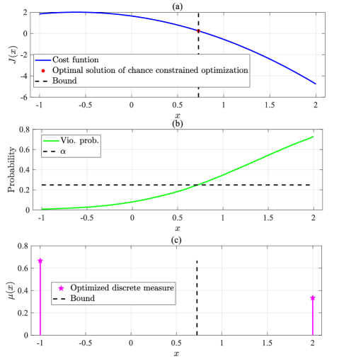
Figure 1: Example in one dimension: (a) profile of $J(x)$ and optimal solution of chance constrained optimization; (b) profile of $1-\mathbb{P}(x)$; (c) optimized discrete measure.

Compared to a deterministic decision, a probabilistic decision can improve performance when chance constraints exist. A simple example is presented here to show the potential improvement of the performance using the probabilistic decision.

Example 1.

The compact set $\mathcal{X}$ is defined by $\mathcal{X}=[-2,2]\subset\mathbb{R}$. The cost function $J(x)$ is

$$J(x)=-(x+0.6)^{2}+2.$$ (6)

The constraint function $h(x,\xi)$ is

$$h(x,\xi)=x-1.4+\xi$$ (7)

where $\xi\sim\mathcal{N}(m_{\xi},\Sigma_{\xi})$ with $m_{\xi}=0$, and $\Sigma_{\xi}=1$. The probability threshold $\alpha$ is $0.25$. The profiles of the objective function $J(x)$ and the violation probability $1-\mathbb{P}(x)$ are plotted in Figure 1 (a) and (b), respectively. In this example, as $x$ increases, the violation probability $1-\mathbb{P}(x)$ increases while the objective function $J(x)$ decreases. Therefore, the optimal solution $x^{*}_{\alpha}$ is at the boundary with $1-\mathbb{P}(x^{*}_{\alpha})=0.25$. Since $\xi$ is a random variable that obeys normal distribution and $h(x,\xi)$ is linear, we can obtain $x^{*}_{\alpha}=0.7259$ from checking the standard normal distribution table, and the corresponding optimal objective value is $J^{*}_{\alpha}=0.2420$.

Then, we explain how probabilistic decisions can further improve the expected objective value. Let $\mathcal{C}_{2}=\{x^{(1)},x^{(2)}\}$ be a set with two samples from $\mathcal{X}=[-2,2]$, where $x^{(1)}=-1$ and $x^{(2)}=2$. The objective function values of these two samples are $J(x^{(1)})=1.84$ and $J(x^{(2)})=-4.76$. The violation probabilities are $\mathbb{P}_{\mathsf{vio}}(x^{(1)})=1-\mathbb{P}(x^{(1)})=0.008$ and $\mathbb{P}_{\mathsf{vio}}(x^{(2)})=1-\mathbb{P}(x^{(2)})=0.729$, respectively. Define a discrete probability measure $\mu$ on $\mathcal{X}=[-2,2]$ with

$$\left\{\begin{array}[]{ll}\mu\left(\{x^{(1)}\}\right)=0.67,\\ \mu\left(\{x^{(2)}\}\right)=0.33.\end{array}\right.$$ (10)

If we choose input probabilistically according to $\mu$, then $x^{(1)}$ is chosen with probability $0.67$ and $x^{(2)}$ is chosen with probability $0.33$. The expected objective value satisfies that

$$J(x^{(1)})\mu\left(\{x^{(1)}\}\right)+J(x^{(2)})\mu\left(\{x^{(2)}\}\right)=-0.338<J^{*}_{\alpha},$$

and the expected violation probability is

$$\mathbb{P}_{\mathsf{vio}}(x^{(1)})\mu\left(\{x^{(1)}\}\right)+\mathbb{P}_{\mathsf{vio}}(x^{(2)})\mu\left(\{x^{(2)}\}\right)=0.2459<\alpha,$$

which implies a probabilistic decision that satisfies the chance constraint can improve the expected control performance compared with the deterministic optimal decision $x^{*}_{\alpha}$.

2.3 Problem formulation of CCPMO

Let $\mathscr{B}(\mathcal{X})$ be Borel $\sigma$-algebra on $\mathcal{X}$. This paper uses $\mathscr{B}(\cdot)$ to denote the Borel $\sigma$-algebra on a metric space. Notice that $\left(\mathcal{X},\mathscr{B}(\mathcal{X})\right)$ is a measurable space (Borel space). Let $\mu$ be a Borel probability measure on $\mathscr{B}(\mathcal{X})$. Besides, let $d$ be Euclidean distance. The ordered pair $\left(\mathcal{X},d\right)$ represents a metric space. Let $M(\mathcal{X})$ be the space of Borel probability measures on metric space $\left(\mathcal{X},d\right)$.

Define a space of continuous $\mathbb{R}$-valued functions on a compact set $\mathcal{X}$ by

$$\mathscr{C}(\mathcal{X}):=\{f:\mathcal{X}\rightarrow\mathbb{R}\,|f\ \text{is continuous}\}.$$ (11)

It is able to define a metric on $\mathscr{C}(\mathcal{X})$ by

$$\tau(f,f^{\prime}):=\|f-f^{\prime}\|_{\infty},\ \forall f,f^{\prime}\in\mathscr{C}(x),$$ (12)

where $\|f\|_{\infty}$ is defined as $\|f\|_{\infty}:=\sup_{x\in\mathcal{X}}|f(x)|.$ The metric $\tau(\cdot,\cdot)$ turns $\mathscr{C}(\mathcal{X})$ into a complete metric space. Define the pseudo-distance (pseudo-metric) between any two probability measures $\mu,\nu\in M(\mathcal{X})$ associated with $f\in\mathscr{C}(\mathcal{X})$ by

$$\mathcal{W}_{f}(\mu,\nu)=\left|\int_{\mathcal{X}}f(x)\mathsf{d}\mu-\int_{\mathcal{X}}f(x)\mathsf{d}\nu\right|.$$ (13)

The weak^∗ convergence of probability measures is defined as follows [30].

Definition 1.

Let $\{\mu_{k}\}_{k=0}^{\infty}$ be a sequence in $M(\mathcal{X})$. We say that $\{\mu_{k}\}_{k=0}^{\infty}$ converges weakly^∗ to $\mu$ if

$$\lim_{k\rightarrow\infty}\mathcal{W}_{f}(\mu_{k},\mu)=0,\ \forall f\in\mathscr{C}(\mathcal{X}).$$ (14)

Besides, we say that $\{\mu_{k}\}_{k=0}^{\infty}$ converges to $\mu$ associated with $f\in\mathscr{C}(\mathcal{X})$ if

$$\lim_{k\rightarrow\infty}\mathcal{W}_{f}(\mu_{k},\mu)=0.$$ (15)

Notice that $h(x,\xi)$ is a random variable for a given $x\in\mathcal{X}$. We introduce an assumption on $h(x,\xi)$ for the continuity analysis of $\mathbb{P}(x)$. Let $\mathsf{cl}\{Z\}$ be the closure of a set $Z$. Let $\mathsf{supp}\ p:=\mathsf{cl}\{\xi\in\Xi:p(\xi)>0\}$, and, for each $x\in\mathcal{X}$,

$$\Xi^{\mathsf{supp}}(x):=\{\xi\in\mathsf{supp}\ p:\bar{h}(x,\xi)=0\}.$$

The following assumption holds throughout the paper.

Assumption 1.

For each $x\in\mathcal{X}$, suppose the following holds:

$$\mathsf{Pr}_{\xi}\{\Xi^{\mathsf{supp}}(x)\}=0.$$

Assumption 1 implies the continuity of $\mathbb{P}(x)$ [21, 31], which guarantees that the feasible set $\mathcal{X}_{\alpha}$ defined by (3) and optimal solution set $X_{\alpha}$ given by (5) are measurable sets for all $\alpha\in[0,1]$.

With the above notation and discussion, a Chance-Constrained Probability Measure Optimization (CCPMO) problem $P_{\alpha}$ associated with Problem $Q_{\alpha}$ can be well formulated as:

$$\underset{\mu\in M(\mathcal{X})}{{\mathsf{min}}}\,\,\int_{\mathcal{X}}J(x)\mathsf{d}\mu P_{\alpha}$$ ()

$${\mathsf{s.t.}}\quad\int_{\mathcal{X}}\mathbb{P}(x)\mathsf{d}\mu\geq 1-\alpha,$$

where $\mathbb{P}(x)$ is defined by (1). In Problem $P_{\alpha}$, the uncertainty of $h(x,\xi)$ comes from both $x$ and $\xi$, since $x$ obeys the distribution dominated by probability measure $\mu$. Let $M_{\alpha}(\mathcal{X})$ be the feasible set of Problem $P_{\alpha}$ by

$$M_{\alpha}(\mathcal{X}):=\Big{\{}\mu\in M(\mathcal{X}):\int_{\mathcal{X}}\mathbb{P}(x)\mathsf{d}\mu\geq 1-\alpha\Big{\}}.$$ (16)

The optimal objective value and the optimal solution set of Problem $P_{\alpha}$ are written as

$$\mathcal{J}^{*}_{\alpha} := \inf_{\mu\in M_{\alpha}(\mathcal{X})}\int_{\mathcal{X}}J(x)\mathsf{d}\mu$$ (17)

$$A_{\alpha} := \Big{\{}\mu\in M_{\alpha}(\mathcal{X}):\int_{\mathcal{X}}J(x)\mathsf{d}\mu=\mathcal{J}^{*}_{\alpha}\Big{\}}.$$ (18)

A probability measure $\mu^{*}_{\alpha}\in A_{\alpha}$ is called an optimal probability measure for Problem $P_{\alpha}$. The optimal probabilistic decision generates a decision at every trial from $\mathcal{X}$ probabilistically according to the optimal probability measure $\mu^{*}_{\alpha}$. If the decision process repeats many times, the mean value of the objective value is minimal.

3 Existence of the optimal solution

In this section, we show that there exists at least an optimal solution to Problem $P_{\alpha}$.

Theorem 1.

Suppose that Assumption 1 holds. Then, we have $A_{\alpha}\neq\emptyset$.

Proof.

The optimal objective value $\mathcal{J}^{*}_{\alpha}$ of Problem $P_{\alpha}$ is defined by (17). We want to prove that there exists at least one $\mu^{*}\in M_{\alpha}(\alpha)$ such that $\int_{\mathcal{X}}J(x)\mathsf{d}\mu^{*}=\mathcal{J}^{*}_{\alpha}$.

For any $\mu\in\mathcal{X}$,

$$\int_{\mathcal{X}}J(x)\mathsf{d}\mu\geq\int_{\mathcal{X}}\min_{x\in\mathcal{X}}\,\,J(x)\mathsf{d}\mu=\min_{x\in\mathcal{X}}\,\,J(x),$$

which implies that $\mathcal{J}^{*}_{\alpha}>-\infty$. Then, there exists a sequence $\{\mu_{k}\}_{k=1}^{\infty}\subset M_{\alpha}(\mathcal{X})$ such that $\int_{\mathcal{X}}J(x)\mathsf{d}\mu_{k}\rightarrow\mathcal{J}^{*}_{\alpha}$. Since $\mathcal{X}$ is compact, by Prokhorov Theorem (Theorem 8.6.2 of [32]), there exists a subsequence $\{\mu_{k_{s}}\}_{s=1}^{\infty}\subset\{\mu_{k}\}_{k=1}^{\infty}$ such that converges weakly^∗ to $\mu^{*}\in M(\mathcal{X})$ in the sense of Definition 1. Since $\int_{\mathcal{X}}J(x)\mathsf{d}\mu_{s_{k}}\rightarrow\int_{\mathcal{X}}J(x)\mathsf{d}\mu^{*}$ by $J(\cdot)\in\mathscr{C}(\mathcal{X})$, we have

$$\int_{\mathcal{X}}J(x)\mathsf{d}\mu^{*}=\lim_{s\to\infty}\int_{\mathcal{X}}J(x)\mathsf{d}\mu_{n_{s}}=\mathcal{J}^{*}_{\alpha}.$$ (19)

We have $\mathbb{P}(\cdot)\in\mathscr{C}(\mathcal{X})$ by Assumption 1. In addition, by $\{\mu_{k}\}_{k=1}^{\infty}\subset M_{\alpha}(\mathcal{X})$, we have $\int_{\mathcal{X}}\mathbb{P}(x)\mathsf{d}\mu_{k_{s}}\geq 1-\alpha,$ for all $s\geq 1$. As a result, since $\mu_{k_{s}}$ converges weakly^∗ to $\mu^{*}$,

$$\int_{\mathcal{X}}\mathbb{P}(x)\mathsf{d}\mu^{*}(x)=\lim_{s\to\infty}\int_{\mathcal{X}}\mathbb{P}(x)\mathsf{d}\mu_{k_{s}}(x)\geq 1-\alpha,$$ (20)

which implies $\mu^{*}\in M_{\alpha}(x)$. By (19) and (20), $\mu^{*}$ is an optimal solution of Problem $P_{\alpha}$ and $A_{\alpha}\neq\emptyset$ holds. ∎

Theorem 1 shows that the optimal solution set $A_{\alpha}$ of Problem $P_{\alpha}$ is not an empty set. The "$\inf$" in (17) can be replaced by "$\min$". Furthermore, we give the following proposition about $\mathcal{J}^{*}_{\alpha}$ and $J^{*}_{\alpha}$.

Proposition 1.

Suppose that Assumption 1 holds. Then,

$$\mathcal{J}^{*}_{\alpha}\leq J^{*}_{\alpha},$$

where $\mathcal{J}^{*}_{\alpha}$ and $J^{*}_{\alpha}$ are the optimal objective values of Problems $P_{\alpha}$ and $Q_{\alpha}$, respectively.

Proof.

Since the optimal solution set $X_{\alpha}$, defined by (5), of Problem $Q_{\alpha}$ is measurable, it is possible to find a probability measure $\tilde{\mu}_{\alpha}\in M(\mathcal{X})$ such that $\tilde{\mu}_{\alpha}(X_{\alpha})=1$. Then, we have

$$\int_{\mathcal{X}}J(x)\mathsf{d}\tilde{\mu}_{\alpha} = \int_{X_{\alpha}}J(x)\mathsf{d}\tilde{\mu}_{\alpha}=J^{*}_{\alpha},$$ (21)

$$\int_{\mathcal{X}}\mathbb{P}(x)\mathsf{d}\tilde{\mu}_{\alpha} = \int_{X_{\alpha}}\mathbb{P}(x)\mathsf{d}\tilde{\mu}_{\alpha}\geq 1-\alpha.$$ (22)

Thus, $\tilde{\mu}_{\alpha}$ is a feasible solution for $P_{\alpha}$ with objective value as $J^{*}_{\alpha}$, namely, $\tilde{\mu}_{\alpha}\in M_{\alpha}(\mathcal{X})$ and $\mathcal{J}^{*}_{\alpha}\leq J^{*}_{\alpha}$. ∎

Proposition 1 shows that the optimal objective value $\mathcal{J}^{*}_{\alpha}$ of Problem $P_{\alpha}$ might be smaller than the optimal objective value $J^{*}_{\alpha}$ of Problem $Q_{\alpha}$. It is necessary to formally investigate in what condition we have $J^{*}_{\alpha}=\mathcal{J}^{*}_{\alpha}$ and how to solve Problem $P_{\alpha}$ when $J^{*}_{\alpha}>\mathcal{J}^{*}_{\alpha}$. We will present corollary 2 in Section 4.1, which gives two sufficient condition for $J^{*}_{\alpha}=\mathcal{J}^{*}_{\alpha}$. For solving Problem $P_{\alpha}$, we first give an equivalent reduction by Theorem 3 in Section 4.1. Then, we extend sample-based smooth approximation to solve the reduced problem in Section 5.

4 Problem Reduction

In this section, we show that there exists an optimal probabilistic decision for Problem $P_{\alpha}$ whose probability measure is concentrated on two points, which leads to an equivalently reduced problem of Problem $P_{\alpha}$.

4.1 Reduced problem of Problem $P_{\alpha}$

We give an assumption on the optimal solution set $A_{\alpha}$.

Assumption 2.

There exists an optimal solution $\mu^{*}\in A_{\alpha}$ of Problem $P_{\alpha}$ such that for any $\delta>0$ there exists a probability measure $\mu$, different from $\mu^{*}$, such that $\int_{\mathcal{X}}\mathbb{P}(x)\mathsf{d}\mu>1-\alpha$ and $\mathcal{W}_{J}(\mu,\mu^{*})\leq\delta$. Here, $\mathcal{W}_{J}(\mu,\mu^{*})$ is the pseudo-distance (pseudo-metric) between $\mu$ and $\mu^{*}$ associated with $J$.

Assumption 2 implies that that there exists a sequence $\{\mu_{k}\}_{k=1}^{\infty}\subseteq M(\mathcal{X})$ that converges to an optimal probability solution $\mu^{*}$ of Problem $P_{\alpha}$ associated with $J$, such that $\int_{\mathcal{X}}\mathbb{P}(x)\mathsf{d}\mu_{k}(x)>1-\alpha$.

Let $\mathcal{C}_{S}=\left(x^{(1)},...,x^{(S)}\right)$ be an element of the augmented space $\mathcal{X}^{S}$, where $S\in\mathbb{N}$. For an arbitrary $\mathcal{C}_{S}$, we can define a set of discrete probability measures by

$$\mathcal{U}_{S}:=\Big{\{}\mu_{S}\in[0,1]^{S}:\sum_{i=1}^{S}\mu_{S}(i)=1\Big{\}}.$$ (23)

The set $\mathcal{C}_{S}$ becomes a sample space with finite samples if it is equipped with a discrete probability measure $\mu_{S}\in\mathcal{U}_{S}$, where the $i$-th element $\mu_{S}(i)$ denotes the probability of taking decision $x^{(i)}$, i.e., $\mu_{S}(x^{(i)})=\mu_{S}(i),i\in[S]$. Thus, by choosing a set $\mathcal{C}_{S}$ and assigning a discrete probability measure $\mu_{S}\in\mathcal{U}_{S}$ to $\mathcal{C}_{S}$, a probabilistic decision is determined, which chooses decision variables from $\mathcal{C}_{S}$ randomly according to $\mu_{S}$. For the probabilistic decision associated with $\mathcal{C}_{S}$ and $\mu_{S}$, the expectations of objective and probability values are $\sum_{i=1}^{S}J(x^{(i)})\mu_{S}(i)$ and $\sum_{i=1}^{S}\mathbb{P}(x^{(i)})\mu_{S}(i)$, respectively. We can optimize $\sum_{i=1}^{S}J(x^{(i)})\mu_{S}(i)$ under a chance constraint $\sum_{i=1}^{S}\mathbb{P}(x^{(i)})\mu_{S}(i)\geq 1-\alpha$ taking $(\mu_{S},\mathcal{C}_{S})$ as decision variable, which is formulated as

$$\min_{\mu_{S}\in\mathcal{U}_{S},\mathcal{C}_{S}\in\mathcal{X}^{S}}\sum_{i=1}^{S}J(x^{(i)})\mu_{S}(i) \tilde{P}_{\alpha}(S)$$ ()

$${\mathsf{s.t.}}\quad\sum_{i=1}^{S}\mathbb{P}(x^{(i)})\mu_{S}(i)\geq 1-\alpha,$$

$$\quad\quad x^{(i)}\in\mathcal{C}_{S},\ \forall i\in[S].$$

Define the feasible set $\tilde{\mathcal{U}}_{\alpha}(S)$ of Problem $\tilde{P}_{\alpha}(S)$ by

$$\tilde{\mathcal{U}}_{\alpha}(S):=\Big{\{}(\mu_{S},\mathcal{C}_{S}):\sum_{i=1}^{S}\mathbb{P}(x^{(i)})\mu_{S}(i)\geq 1-\alpha\Big{\}}.$$ (24)

Since the objective function $\sum_{i=1}^{S}\mathbb{P}(x^{(i)})\mu_{S}(i):\mathcal{U}_{S}\times\mathcal{X}^{S}\to R$ is continuous, and its domain $\mathcal{U}_{S}\times\mathcal{X}^{S}$ is compact, we have the feasible set $\tilde{\mathcal{U}}_{\alpha}(S)$ of Problem $\tilde{P}_{\alpha}(S)$ is also a compact set. As a result, problem $\tilde{P}_{\alpha}(S)$’s optimal solution exists. Define the optimal objective value $\tilde{\mathcal{J}}_{\alpha}(S)$ of Problem $\tilde{P}_{\alpha}(S)$ by

$$\tilde{\mathcal{J}}_{\alpha}(S):=\min_{(\mu_{S},\mathcal{C}_{S})\in\tilde{\mathcal{U}}_{\alpha}(S)}\sum_{i=1}^{S}J(x^{(i)})\mu_{S}(i).$$ (25)

The optimal solution set of Problem $\tilde{P}_{\alpha}(S)$ is written as

$$\tilde{A}_{\alpha}(S):=\Big{\{}(\mu_{S},\mathcal{C}_{S})\in\tilde{\mathcal{U}}_{\alpha}(S):\sum_{i=1}^{S}J(x^{(i)})\mu_{S}(i)=\tilde{\mathcal{J}}_{\alpha}(S)\Big{\}}.$$

For $\tilde{\mathcal{J}}_{\alpha}(S)$, we have the following theorem.

Theorem 2.

Suppose that Assumptions 1 and 2 hold. We have

$$\lim_{S\rightarrow\infty}\tilde{\mathcal{J}}_{\alpha}(S)=\mathcal{J}^{*}_{\alpha}.$$ (26)

The proof of Theorem 2 is presented in Appendix A. If the number $S\rightarrow\infty$, the optimal solution $\tilde{\mu}_{S}\in\tilde{A}_{\alpha}(S)$ of Problem $\tilde{P}_{\alpha}(S)$ can be used as an approximate optimal solution of Problem $P_{\alpha}$. However, solving Problem $\tilde{P}_{\alpha}(S)$ becomes computationally impractical when $S\rightarrow\infty$. We will further show that the optimal objective value $\tilde{\mathcal{J}}_{\alpha}(S)$ equals $\mathcal{J}^{*}_{\alpha}$ when $S=2$.

Let

$$\mathcal{U}_{\mathsf{m}}:=\Big{\{}\mu_{\mathsf{m}}\in[0,1]^{2}:\sum_{i=1}^{2}\mu_{\mathsf{m}}(i)=1\Big{\}}.$$ (27)

Let $\bm{z}_{\mathsf{m}}:=\left(\mu_{\mathsf{m}}(1),\mu_{\mathsf{m}}(2),\bm{x}_{\mathsf{m}}(1),\bm{x}_{\mathsf{m}}(2)\right)$ be a variable in the set $\mathcal{Z}_{\mathsf{m}}:=\mathcal{U}_{\mathsf{m}}\times\mathcal{X}^{2}$. Then, consider an optimization problem on $\bm{z}_{\mathsf{m}}$ written as

$$\min_{\bm{z}_{\mathsf{m}}\in\mathcal{Z}_{\mathsf{m}}}\,\,\sum_{i=1}^{2}J(x^{(i)})\mu_{\mathsf{m}}(i) W_{\alpha}$$ ()

$$\mathsf{s.t.}\quad\sum_{i=1}^{2}\mu_{\mathsf{m}}(i)\mathbb{P}(x^{(i)})\geq 1-\alpha.$$

Define the feasible set $Z_{\mathsf{m},\alpha}$ of Problem $W_{\alpha}$ by

$$\mathcal{Z}_{\mathsf{m},\alpha}:=\Big{\{}\bm{z}_{\mathsf{m}}\in\mathcal{Z}_{\mathsf{m}}:\sum_{i=1}^{2}\mathbb{P}(x^{(i)})\mu_{\mathsf{m}}(i)\geq 1-\alpha\Big{\}}.$$

In addtion, define the optimal objective value $\mathcal{J}^{\mathsf{w}}_{\alpha}$ and optimal solution set $D_{\alpha}$ of Problem $W_{\alpha}$ by

$$\mathcal{J}^{\mathsf{w}}_{\alpha} :=\min\Big{\{}\sum_{i=1}^{2}J(x^{(i)})\mu_{\mathsf{m}}(i):\bm{z}_{\mathsf{m}}\in\mathcal{Z}_{\mathsf{m},\alpha}\Big{\}},$$ (28)

$$D_{\alpha} :=\Big{\{}\bm{z}_{\mathsf{m}}\in\mathcal{Z}_{\mathsf{m},\alpha}:\sum_{i=1}^{2}J(x^{(i)})\mu_{\mathsf{m}}(i)=\mathcal{J}^{\mathsf{w}}_{\alpha}\Big{\}},$$ (29)

respectively. Notice that Problem $W_{\alpha}$ is a special case of Problem $\tilde{P}_{\alpha}(S)$ with $S=2$. We redefine it as Problem $W_{\alpha}$ to simplify the notation in Section 5 for the convenience of discussing the approximate problem established by extracting samples of $\xi$. The following theorem shows that the optimal objective values of Problem $W_{\alpha}$ and Problem $P_{\alpha}$ are equal.

Theorem 3.

Suppose Assumptions 1-2 hold. Then, we have $\mathcal{J}^{*}_{\alpha}=\mathcal{J}^{\mathsf{w}}_{\alpha}$.

The proof of Theorem 3 is summarized in Section 4.2. Theorem 3 is the main result for establishing a reduced problem $W_{\alpha}$ equivalent to Problem $P_{\alpha}$. Namely, to obtain an optimal probabilistic decision, instead of solving Problem $P_{\alpha}$, an optimization problem in an infinite-dimensional space, we could solve problem $W_{\alpha}$ whose domain is $[0,1]^{2}\times\mathcal{X}^{2}$ in the $(2n+2)$-dimension space.

Let $\bm{z}_{\mathsf{m}}^{*}\in D_{\alpha}$ be an optimal solution of Problem $W_{\alpha}$. The solution $\bm{z}_{\mathsf{m}}^{*}$ is written as $\bm{z}_{\mathsf{m}}^{*}:=\left(\mu_{\mathsf{m}}^{*}(1),\mu_{\mathsf{m}}^{*}(2),x_{*}^{(1)},x_{*}^{(2)}\right)$, where $\mu_{\mathsf{m}}^{*}(1),\mu_{\mathsf{m}}^{*}(2)$ are assigned to $x_{*}^{(1)},x_{*}^{(2)}$, respectively. Define a mapping from the optimal solution set $D_{\alpha}$ of Problem $W_{\alpha}$ to the domain $M(\mathcal{X})$ of Problem $P_{\alpha}$, as $\Phi:D_{\alpha}\rightarrow M(\mathcal{X})$, for any $\bm{z}^{*}_{\mathsf{m}}\in D_{\alpha}$, we obtain a probability measure

$$\tilde{\mu}_{\bm{z}^{*}_{\mathsf{m}}}=\Phi(\bm{z}^{*}_{\mathsf{m}})\in M(\mathcal{X})$$

that satisfies $\tilde{\mu}_{\bm{z}^{*}_{\mathsf{m}}}(\{x^{(1)}_{*}\})=\mu^{*}_{\mathsf{m}}(1)$ and $\tilde{\mu}_{\bm{z}^{*}_{\mathsf{m}}}(\{x^{(2)}_{*}\})=\mu^{*}_{\mathsf{m}}(2)$. By Theorem 3, we have

$$\int_{\mathcal{X}}J(x)\mathsf{d}\tilde{\mu}_{\bm{z}^{*}_{\mathsf{m}}}(x)=\sum_{i=1}^{2}J(x^{(i)}_{*})\mu^{*}_{\mathsf{m}}(i)=\mathcal{J}^{*}_{\alpha}.$$ (30)

In addition, if $\bm{z}_{\mathsf{m}}^{*}\in D_{\alpha}$ is an optimal solution of Problem $W_{\alpha}$, we have

$$\int_{\mathcal{X}}\mathbb{P}(x)\mathsf{d}\tilde{\mu}_{\bm{z}^{*}_{\mathsf{m}}}(x)=\sum_{i=1}^{2}\mathbb{P}(x^{(i)}_{*})\mu^{*}_{\mathsf{m}}(i)\geq 1-\alpha.$$ (31)

From (30) and (31), we have that $\tilde{\mu}_{\bm{z}^{*}_{\mathsf{m}}}$ is within the optimal set $A_{\alpha}$ of Problem $P_{\alpha}$. Namely, by solving Problem $W_{\alpha}$, we could obtain an optimal solution $\tilde{\mu}_{\bm{z}^{*}_{\mathsf{m}}}$ of Problem $P_{\alpha}$ through the mapping $\Phi$.

Besides, we summarize the properties of the optimal solutions of Problem $W_{\alpha}$ in the following corollary.

Corollary 1.

Let $\bm{z}_{\mathsf{m}}^{*}=\left(\mu_{\mathsf{m}}^{*}(1),\mu_{\mathsf{m}}^{*}(2),x^{(1)}_{*},x^{(2)}_{*}\right)\in D_{\alpha}$ be an optimal solution of Problem $W_{\alpha}$. Let $\tilde{\alpha}^{(1)}=1-\mathbb{P}(x^{(1)}_{*})$ and $\tilde{\alpha}^{(2)}=1-\mathbb{P}(x^{(2)}_{*})$. We have $x^{(1)}_{*}\in X_{\tilde{\alpha}^{(1)}},x^{(2)}_{*}\in X_{\tilde{\alpha}^{(2)}}$.

The proof of Corollary 1 is presented in Appendix B. By Corollary 1, the optimal solution of Problem $W_{\alpha}$ contains two points in $\mathcal{X}$ such that are optimal solutions of $Q_{\tilde{\alpha}^{(1)}}$ and $Q_{\tilde{\alpha}^{(2)}}$, respectively. The following corollary summarizes the connections between Problem $P_{\alpha}$ and Problem $Q_{\alpha}$.

Corollary 2.

If $J^{*}_{\tilde{\alpha}}$ is a convex function of $\tilde{\alpha}$ or when $\alpha=0$, we have $\mathcal{J}^{*}_{\alpha}=J^{*}_{\alpha}$.

The proof of Corollary 2 is presented in Appendix C. Corollary 2 shows that it is not necessary to consider chance constrained probability measure optimization for improving the expectation of the performance under the chance constraint when $J^{*}_{\tilde{\alpha}}$ is a convex function of $\tilde{\alpha}$ or $\alpha=0$. We cannot verify whether $J^{*}_{\tilde{\alpha}}$ is a convex function of $\tilde{\alpha}$ in advance. When $\alpha=0$, the constraint $\bar{h}(x,\xi)$ should be satisfied with probability 1 (w.p.1). In this case, the deterministic decision can achieve the optimal solution, and the probabilistic decision is unnecessary.

4.2 Proof of Theorem 3

For a given number $S\in\mathbb{N}$, let $\mathcal{E}_{S}:=\left(\tilde{\alpha}^{(1)},...,\tilde{\alpha}^{(S)}\right)$ be an element of $[0,1]^{S}$, defining as a set of violation probabilities, where each $\tilde{\alpha}^{(i)}$ is a threshold of violation probability in Problem $Q_{\tilde{\alpha}^{(i)}}$ (Problem $Q_{\alpha}$ when $\alpha=\tilde{\alpha}^{(i)}$). For a violation probability set $\mathcal{E}_{S}$, we have a corresponding optimal objective value set $\{J^{*}_{\tilde{\alpha}^{(1)}},...,J^{*}_{\tilde{\alpha}^{(i)}},...,J^{*}_{\tilde{\alpha}^{(S)}}\}$, where $J^{*}_{\tilde{\alpha}^{(i)}}$ is the optimal objective value $J^{*}_{\tilde{\alpha}^{(i)}}$ of Problem $Q_{\tilde{\alpha}^{(i)}}$, for a given $\tilde{\alpha}^{(i)}$, by (4). Let $\mathcal{V}_{S}:=\{\nu_{S}\in[0,1]^{S}:\sum_{i=1}^{S}\nu_{S}(i)=1\}$ be a set of discrete probability measures that defined on $\mathcal{E}_{S}$. By determining a violation probability set $\mathcal{E}_{S}$ and assigning a discrete probability $\nu_{S}$ to $\mathcal{E}_{S}$, we get a probabilistic decision in which the threshold of violation probability is randomly extracted from $\mathcal{E}_{S}$ obeying the discrete probability $\nu_{S}$. The corresponding expectation of the optimal objective value is $\sum_{i=1}^{S}J^{*}_{\tilde{\alpha}^{(i)}}\nu_{S}(i)$. The expectation of the objective value can be optimized under a chance constraint $\sum_{i=1}^{S}(1-\tilde{\alpha}^{(i)})\nu_{S}(i)\geq 1-\alpha$ taking $(\nu_{S},\mathcal{E}_{S})$ as the decision variable, which is formulated as

$$\min_{\nu_{S}\in\mathcal{V}_{S},\mathcal{E}_{S}\in[0,1]^{S}}\,\,\sum_{i=1}^{S}J^{*}_{\tilde{\alpha}^{(i)}}\nu_{S}(i) \tilde{V}_{\alpha}(S)$$ ()

$${\mathsf{s.t.}}\quad\sum_{i=1}^{S}(1-\tilde{\alpha}^{(i)})\nu_{S}(i)\geq 1-\alpha,$$

$$\quad\quad\ \tilde{\alpha}^{(i)}\in\mathcal{E}_{S},\ \forall i\in[S].$$

In this cost function of Problem $\tilde{V}_{\alpha}(S)$, the optimal objective value $J^{*}_{\tilde{\alpha}^{(i)}}$ of Problem $Q_{\tilde{\alpha}^{(i)}}$ is used for each $\tilde{\alpha}^{(i)}$, which is the same as $J(x^{(i)})$ for each $x^{(i)}$ in Problem $\tilde{P}_{\alpha}(S)$. For the simplicity of writing, we use the notations $\bm{\theta}_{S}:=(\nu_{S},\mathcal{E}_{S})$ and $\Theta_{S}:=\mathcal{V}_{S}\times[0,1]^{S}$. Define the feasible set $\Theta_{S,\alpha}$ of $\tilde{V}_{\alpha}(S)$ by

$$\Theta_{S,\alpha}:=\Big{\{}\bm{\theta}_{S}\in\Theta_{S}:\sum_{i=1}^{S}(1-\tilde{\alpha}^{(i)})\nu_{S}(i)\geq 1-\alpha\Big{\}}.$$

Different from Problem $\tilde{P}_{\alpha}(S)$, Problem $\tilde{V}_{\alpha}(S)$ optimizes finite combinations of violation probability thresholds to achieve the minimal mean optimal objective value with chance constraint. We summarize the connection between $\tilde{P}_{\alpha}(S)$ and $\tilde{V}_{\alpha}(S)$ in Proposition 2.

Proposition 2.

Suppose Assumption 1 holds. For all $S\in\mathbb{N}$, there exists a feasible solution $\bm{\theta}_{S}:=(\nu_{S},\tilde{\alpha}^{(1)},...,\tilde{\alpha}^{(S)})\in\Theta_{S,\alpha}$ of Problem $\tilde{V}_{\alpha}(S)$ that satisfies

$$\sum_{i=1}^{S}J^{*}_{\tilde{\alpha}^{(i)}}\nu_{S}(i)=\tilde{\mathcal{J}}_{\alpha}(S),$$ (32)

where $\tilde{\mathcal{J}}_{\alpha}(S)$ is the optimal objective value of Problem $\tilde{P}_{\alpha}(S)$ defined by (25).

The proof of Proposition 2 is presented in Appendix D. By using Proposition 2, we can further obtain the following lemma.

Lemma 1.

Suppose Assumptions 1-2 both hold. There exists a feasible solution $\bm{\theta}_{\mathsf{m}}:=\{\nu_{\mathsf{m}}(1),\nu_{\mathsf{m}}(2),\tilde{\alpha}_{\mathsf{m}}^{(1)},\tilde{\alpha}_{\mathsf{m}}^{(2)}\}\in\Theta_{2,\alpha}$ of Problem $\tilde{V}_{\alpha}(2)$ that satisfies

$$\sum_{i=1}^{2}J^{*}_{\tilde{\alpha}_{\mathsf{m}}^{(i)}}\nu_{\mathsf{m}}(i)=\mathcal{J}^{*}_{\alpha}.$$ (33)

The proof of Lemma 1 is presented in Appendix E. With Theorem 2 and Lemma 1 as the preparation, the proof of Theorem 3 is summarized as follows:

Proof.

By (48) in the Proof of Theorem 2 (Appendix A), we have $\mathcal{J}^{*}_{\alpha}\leq\mathcal{J}^{\mathsf{w}}_{\alpha}$, where $\mathcal{J}^{\mathsf{w}}_{\alpha}=\tilde{J}_{\alpha}(S)$ with $S=2$. Then, we need to show that $\mathcal{J}^{*}_{\alpha}\geq\mathcal{J}^{\mathsf{w}}_{\alpha}$. By Lemma 1, we can find a feasible solution $\bm{\theta}_{\mathsf{m}}:=\{\nu_{\mathsf{m}}(1),\nu_{\mathsf{m}}(2),\tilde{\alpha}_{\mathsf{m}}^{(1)},\tilde{\alpha}_{\mathsf{m}}^{(2)}\}\in\Theta_{2,\alpha}$ of Problem $\tilde{V}_{\alpha}(S)$ with $S=2$ that satisfies (33), namely, $\mathcal{J}^{*}_{\alpha}=\sum_{i=1}^{2}J_{\tilde{\alpha}^{(i)}_{\mathsf{m}}}^{*}\nu_{\mathsf{m}}(i)$. Choose $\mu_{\mathsf{m}}=\nu_{\mathsf{m}}$ and $x^{(1)}_{*}\in X_{\tilde{\alpha}^{(1)}_{\mathsf{m}}},\ x^{(2)}_{*}\in X_{\tilde{\alpha}^{(2)}_{\mathsf{m}}}$. Since $\bm{\theta}_{\mathsf{m}}$ is a feasible solution of Problem $\tilde{V}_{\alpha}(2)$, we have

$$\sum_{i=1}^{2}\mathbb{P}(x^{(i)}_{*})\mu_{\mathsf{m}}(i)\geq\sum_{i=1}^{2}\left(1-\tilde{\alpha}^{(i)}_{\mathsf{m}}\right)\nu_{\mathsf{m}}(i)\geq 1-\alpha.$$ (34)

Notice that (34) implies that $\left(\mu_{\mathsf{m}}(1),\mu_{\mathsf{m}}(2),x^{(1)}_{*},x^{(2)}_{*}\right)$ is a feasible solution of Problem $W_{\alpha}$. By Lemma 1, we have

$$\mathcal{J}^{*}_{\alpha}=\sum_{i=1}^{2}J_{\tilde{\alpha}^{(i)}_{\mathsf{m}}}^{*}\nu_{\mathsf{m}}(i)=\sum_{i=1}^{2}J(x^{(i)}_{*})\mu_{\mathsf{m}}(i)\geq\mathcal{J}^{\mathsf{w}}_{\alpha}.$$ (35)

Thus, we have $\mathcal{J}^{\mathsf{w}}_{\alpha}=\mathcal{J}^{*}_{\alpha}$. ∎

Here, we give a simple numerical example to demonstrate the result of Theorem 3 as follows:

Example 2.

The cost function $J(x)$ and the constraint function $h(x,\xi)$ are given by (6) and (7) in Example 1 , respectively. For $\alpha=0.25$, we obtain $\tilde{J}_{\alpha}(S)$ for $S=1,2,5,10,20,30,50$. The result is plotted in Figure 2. As illustrated by Figure 2, the optimal probabilistic decision with the probability measure concentrated on two points achieves the same cost performance as the ones with the probability measure concentrated on more points, consistent with Theorem 3. The problem $\tilde{P}_{\alpha}(S)$ is solved by the sample-based smooth approximation method presented in Section 5. Although the case with $S=2$ is discussed in Section 5, the conclusions are consistent for any finite integer $S$.

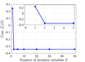
Figure 2: Demonstration of the result of Theorem 3.

5 Sample-based smooth approximation for Solving Problem $W_{\alpha}$

Section 4 has shown that Problem $P_{\alpha}$ has an optimal probabilistic decision whose probability measure is concentrated on two points. By solving Problem $W_{\alpha}$ whose domain is $(2n+2)$-dimensional, we can obtain an optimal solution of Problem $P_{\alpha}$. However, due to chance constraints from the random variable $\xi$ (refer to (1) and (2)), Problem $W_{\alpha}$ is still an intractable problem. This section presents the approximate method for solving Problem $W_{\alpha}$ by extracting samples from $\Xi$.

5.1 Uniform convergence of optimal objective values

As with [20], we have the following assumption on problem $Q_{\alpha}$ for every $\alpha\in(0,1]$.

Assumption 3.

For all $\alpha\in(0,1]$, there exists a globally optimal solution of $Q_{\alpha}$, $\bar{x}_{\alpha}$, such that for any $\eta>0$ there is $x\in\mathcal{X}$ such that $\|x-\bar{x}_{\alpha}\|\leq\eta$ and $\mathbb{P}(x)>1-\alpha$.

Assumption 3 implies that there exists a sequence $\{x_{k}\}_{k=1}^{\infty}\subset\mathcal{X}$ that converges to an optimal solution $\bar{x}_{\alpha}$ of Problem $Q_{\alpha}$ such that $\mathbb{P}(x_{k})>1-\alpha$. Recall that the constraint function $h(x,\xi)$ of Problem $Q_{\alpha}$ involves the random variable $\xi$. The sample space of $\xi$ is $\Xi$. Let $\mathcal{D}_{N}=\{\xi^{(1)},...,\xi^{(N)}\}$ be a set of samples, where $\xi^{(j)},j\in[N]$ is extracted from $\Xi$, the support of $\xi$. With data set $\mathcal{D}_{N}$, we can define a sample-based approximation of $\mathbb{P}(x)$ by

$$\hat{\mathbb{P}}_{N}(x):=\frac{1}{N}\sum_{j=1}^{N}\mathbb{I}\left(h(x,\xi^{(j)})\right).$$ (36)

There is one drawback to using the sample-based approximation. The sample-based approximation is not differentiable due to the discontinuous indicator function $\mathbb{I}(\cdot)$.

As in [20], for a positive parameter $\varepsilon$, a function $\Lambda_{\varepsilon}(\cdot)$ is defined

$$\Lambda_{\varepsilon}(y)=\left\{\begin{array}[]{ll}0,&y\geq\varepsilon,\\ \lambda_{\varepsilon}(y),&-\varepsilon<y<\varepsilon,\\ 1,&\mbox{if}\ y\leq-\varepsilon,\end{array}\right.$$ (40)

where $\lambda_{\varepsilon}:[-\varepsilon,\varepsilon]\rightarrow[0,1]$ is a symmetric and strictly decreasing smooth function that makes $\Lambda_{\varepsilon}(\cdot)$ a continuously differentiable function. For a smoothing parameter $\varepsilon>0$, sample number $N>0$, a positive parameter $\gamma>0$, we define $\tilde{\mathbb{P}}^{\gamma,\varepsilon}_{N}(x)$ by

$$\tilde{\mathbb{P}}^{\gamma,\varepsilon}_{N}(x):=\frac{1}{N}\sum_{j=1}^{N}\Lambda_{\varepsilon}\left(h(x,\xi^{(j)})+\gamma\right).$$ (41)

The function $\tilde{\mathbb{P}}^{\gamma,\varepsilon}_{N}(x)$ is a sample-based smooth approximation of $\mathbb{P}(x)$. Compared to the sample-based approximation $\hat{\mathbb{P}}_{N}(x)$, $\tilde{\mathbb{P}}^{\gamma,\varepsilon}_{N}(x)$ is differentiable and gives a smooth approximation of feasible region’s boundary.

For a given set $\mathcal{D}_{N}$, positive parameters $\alpha^{\prime}\in[0,\alpha),\gamma,\varepsilon>0$, a sample-based smooth approximate problem of $W_{\alpha}$ is formulated as:

$$\min_{\bm{z}_{\mathsf{m}}}\sum_{i=1}^{2}J(x^{(i)})\mu_{\mathsf{m}}(i) \tilde{W}_{\alpha^{\prime}}^{\gamma,\varepsilon}(\mathcal{D}_{N})$$ ()

$${\mathsf{s.t.}}\quad\sum_{i=1}^{2}\tilde{\mathbb{P}}^{\gamma,\varepsilon}_{N}(x^{(i)})\mu_{\mathsf{m}}(i)\geq 1-\alpha^{\prime}.$$

Let $\mathcal{J}_{\mathsf{m}}(\bm{z}_{\mathsf{m}}):=\sum_{i=1}^{2}J(x^{(i)})\mu_{\mathsf{m}}(i)$ and $\mathcal{P}_{\mathsf{m}}(\bm{z}_{\mathsf{m}}):=\sum_{i=1}^{2}\tilde{\mathbb{P}}^{\gamma,\varepsilon}_{N}(x^{(i)})\mu_{\mathsf{m}}(i)$. The feasible region $\mathcal{Z}_{\mathsf{m},\alpha^{\prime}}^{\gamma,\varepsilon}(\mathcal{D}_{N})$, the optimal objective value $\tilde{\mathcal{J}}_{\alpha^{\prime}}^{\gamma,\varepsilon}(\mathcal{D}_{N})$, and the optimal solution set $\tilde{D}_{\alpha^{\prime}}^{\gamma,\varepsilon}(\mathcal{D}_{N})$ of Problem $\tilde{W}_{\alpha^{\prime}}^{\gamma,\varepsilon}(\mathcal{D}_{N})$ are defined by

$$\mathcal{Z}_{\mathsf{m},\alpha^{\prime}}^{\gamma,\varepsilon}(\mathcal{D}_{N}) =\Big{\{}\bm{z}_{\mathsf{m}}\in\mathcal{Z}_{\mathsf{m}}:\mathcal{P}_{\mathsf{m}}(\bm{z}_{\mathsf{m}})\geq 1-\alpha^{\prime}\Big{\}}$$ (42)

$$\tilde{\mathcal{J}}_{\alpha^{\prime}}^{\gamma,\varepsilon}(\mathcal{D}_{N}) =\min_{\bm{z}_{\mathsf{m}}\in\mathcal{Z}_{\mathsf{m},\alpha^{\prime}}^{\gamma,\varepsilon}(\mathcal{D}_{N})}\mathcal{J}_{\mathsf{m}}(\bm{z}_{\mathsf{m}})$$

$$\tilde{D}_{\alpha^{\prime}}^{\gamma,\varepsilon}(\mathcal{D}_{N}) =\left\{\bm{z}_{\mathsf{m}}\in\mathcal{Z}_{\mathsf{m},\alpha^{\prime}}^{\gamma,\varepsilon}(\mathcal{D}_{N}):\mathcal{J}_{\mathsf{m}}(\bm{z}_{\mathsf{m}})=\tilde{\mathcal{J}}_{\alpha^{\prime}}^{\gamma,\varepsilon}(\mathcal{D}_{N})\right\}.$$

The uniform convergence in the sense of almost everywhere on $\tilde{\mathcal{J}}_{\alpha^{\prime}}^{\gamma,\varepsilon}(\mathcal{D}_{N})$ and $\tilde{D}_{\alpha^{\prime}}^{\gamma,\varepsilon}(\mathcal{D}_{N})$ is summarized in the following theorem.

Theorem 4.

Suppose Assumptions 1-3 hold. If $\gamma=0$, as $N\rightarrow\infty$, and $\varepsilon\rightarrow 0$, we have $\tilde{\mathcal{J}}_{\alpha}^{\gamma,\varepsilon}(\mathcal{D}_{N})\rightarrow\mathcal{J}^{*}_{\alpha}$ and $\mathbb{D}\left(\tilde{D}_{\alpha}^{\gamma,\varepsilon}(\mathcal{D}_{N}),D_{\alpha}\right)\rightarrow 0$  w. p. 1, where

$$\mathbb{D}(Z_{1},Z_{2}):=\sup_{z\in Z_{1}}\inf_{z^{\prime}\in Z_{2}}\|z-z^{\prime}\|$$

is the deviation of set $Z_{1}$ from set $Z_{2}$.

The proof of Theorem 4 is presented in Appendix F.

5.2 Feasibility with finite samples

Then, now consider the condition under which an optimal solution for Problem $\tilde{W}_{\alpha^{\prime}}^{\gamma,\varepsilon}(\mathcal{D}_{N})$ is feasible for Problem $W_{\alpha}$. Define $\hat{\mathbb{P}}^{\gamma,\varepsilon}(x)$ for $x\in\mathcal{X}$ by

$$\hat{\mathbb{P}}^{\gamma,\varepsilon}(x):=\int_{\Xi}\Lambda_{\varepsilon}\left(h(x,\xi)+\gamma\right)p(\xi)\mathsf{d}\xi.$$ (44)

We have the probabilistic feasibility guarantee as stated in the following theorem.

Theorem 5.

Let $\tilde{\bm{z}}_{\mathsf{m},\alpha^{\prime}}\in\tilde{D}^{\gamma,\varepsilon}_{\alpha^{\prime}}(\mathcal{D}_{N})$ be an optimal solution of Problem $\tilde{W}_{\alpha^{\prime}}^{\gamma,\varepsilon}(\mathcal{D}_{N})$, which is specified as $\tilde{\bm{z}}_{\mathsf{m},\alpha^{\prime}}=\left(\tilde{\mu}_{\mathsf{m}}(1),\tilde{\mu}_{\mathsf{m}}(2),\tilde{x}^{(1)},\tilde{x}^{(2)}\right)$. Then, if $\alpha^{\prime}<\alpha$ we have

$$\mathsf{Pr}\{\tilde{\bm{z}}_{\mathsf{m},\alpha^{\prime}}\notin\mathcal{Z}_{\mathsf{m},\alpha}\}\leq\exp\{-2N\left(R^{\gamma,\varepsilon}_{\alpha^{\prime}}\right)^{2}\},$$ (45)

where $R^{\gamma,\varepsilon}_{\alpha^{\prime}}$ is defined by

$$R^{\gamma,\varepsilon}_{\alpha^{\prime}}\!=\!\inf_{\bm{z}_{\mathsf{m}}\in\mathcal{Z}_{\mathsf{m}}}\sum_{i=1}^{2}\left(\mathbb{P}(x^{(i)})-\hat{\mathbb{P}}^{\gamma,\varepsilon}(x^{(i)})\right)\mu_{\mathsf{m}}(i)+(\alpha-\alpha^{\prime}).$$ (46)

The proof of Theorem 5 is presented in Appendix G. Theorem 5 shows that if the violation probability threshold of the approximate Problem $\tilde{W}_{\alpha^{\prime}}^{\gamma,\varepsilon}(\mathcal{D}_{N})$ is decreased appropriately to $\alpha^{\prime}<\alpha$, then an optimal solution $\tilde{\bm{z}}_{\mathsf{m},\alpha^{\prime}}$ of the approximate problem $\tilde{W}_{\alpha^{\prime}}^{\gamma,\varepsilon}(\mathcal{D}_{N})$ is not feasible for Problem $W_{\alpha}$ with a probability that decreases exponentially with the size of the sample $N$.

6 Numerical Validation

In this section, numerical validations have been implemented to compare the performances of the proposed probabilistic decision method and several existing deterministic decision methods. The chosen application case study is a chance-constrained trajectory planning problem with obstacles, a very common industrial problem in trajectory planning of autonomous driving [34]. Note that we use a simplified model used in [35] for this demonstration.

6.1 Model and simulation settings

The numerical example considers a quadrotor system control problem in turbulent conditions. The control problem is expressed as follows:

$$\underset{\mu\in M(\mathcal{U}^{N})}{{\mathsf{min}}}\,\,\mathcal{J}(\mu)=\mathbb{E}\{\ell^{s}(s)+\ell^{u}(u)\} P_{\mathsf{QSC}}$$ ()

$${\mathsf{s.t.}}\quad s_{t+1}=As_{t}+B(m)u_{t}+d(s_{t},\varphi)+\omega_{t},\ u\sim M(\mathcal{U}^{N}),$$

$$\ \ \ \ \quad t=0,1,...,N-1,$$

$$\ \ \ \ \quad\mathsf{Pr}\{\left(\land_{t=1}^{N-1}s_{t}\notin\mathcal{O}\right)\land(s_{N}\in\mathcal{S}_{\mathsf{goal}})\}\geq 1-\alpha,$$

where $A$, $B(m)$, $d(s_{t},\varphi)$ are written by

$$A=\begin{bmatrix}1&\Delta t&0&0\\ 0&1&0&0\\ 0&0&1&\Delta t\\ 0&0&0&1\end{bmatrix},\ B(m)=\frac{1}{m}\begin{bmatrix}\frac{\Delta t^{2}}{2}&0\\ \Delta t&0\\ 0&\frac{\Delta t^{2}}{2}\\ 0&\Delta t\end{bmatrix},\$$

$d(s_{t},\varphi)=-\varphi[\frac{\Delta t^{2}|v_{x}|v_{x}}{2}\ \Delta t|v_{x}|v_{x}\ \frac{\Delta t^{2}|v_{y}|v_{y}}{2}\ \Delta t|v_{y}|v_{y}]^{\top}$ and $\Delta t=1$ is the sampling time, the state of the system is denoted as $s_{t}=[p_{x,t},v_{x,t},p_{y,t},v_{y,t}]\in\mathbb{R}^{4}$, the control input of the system is $u_{t}=\{u_{x},u_{y}\}$, and the state and control trajectories are denoted as $s=(s_{t})_{t=1}^{N}$ and $u=(u_{t})_{t=1}^{N-1}$. The system starts from an initial point $s_{0}=[-0.5,0,-0.5,0]$. The system is expected to reach the destination set $\mathcal{S}_{\mathsf{goal}}=\{(p_{x},v_{x},p_{y},v_{y})|\|(p_{x}-10,p_{y}-10)\|\leq 2,v_{x}=0,v_{y}=0\}$ at time $N=10$ while avoiding two polytopic obstacles $\mathcal{O}$ shown in Fig. 3. The dynamics are parametrized by uncertain parameter vector $\xi_{t}=[m,\varphi]^{\top}$, where $m>0$ represents the system’s mass and $\varphi>0$ is an uncertain drag coefficient. The parameter vector $\xi$ of the system is uncorrelated random variables such that $(m-0.75)/0.5\sim\mathsf{Beta}(2,2)$ and $(\varphi-0.4)/0.2\sim\mathsf{Beta}(2,5)$, where $\mathsf{Beta}(a,b)$ denotes a Beta distribution with shape parameters $(a,b)$. $\omega_{t}\in\mathbb{R}^{4}$ is the uncertain disturbance at time step $t$, which obeys multivariate normal distribution with zero means and a diagonal covariance matrix $\Sigma$ with the diagonal elements as $\Sigma(1,1)=0.01,\ \Sigma(2,2)=0.75,\ \Sigma(3,3)=0.01,\ \Sigma(4,4)=0.75$. The cost function includes

• $\ell^{s}(s)=\frac{1}{N}\sum_{t=0}^{N-1}\left((p_{x,t+1}-p_{x,t})^{2}+(p_{y,t+1}-p_{y,t})^{2}\right)$;

• $\ell^{u}(u)=\frac{0.1}{N}\sum_{t=0}^{N-1}\left(u_{1,t}^{2}+u_{2,t}^{2}\right)$.

By solving Problem $P_{\mathsf{QSC}}$, we could get probability measure $\mu$ to implement a probabilistic decision. For deterministic decision, the following problem should be solved instead.

$$\underset{u\in\mathcal{U}^{N}}{{\mathsf{min}}}\,\,J(u)=\mathbb{E}\{\ell^{s}(s)+\ell^{u}(u)\} P_{\mathsf{QSC}}^{\mathsf{det}}$$ ()

$${\mathsf{s.t.}}\quad s_{t+1}=As_{t}+B(m)u_{t}+d(s_{t},\varphi)+\omega_{t},\ u\sim M(\mathcal{U}^{N}),$$

$$\ \ \ \ \quad t=0,1,...,N-1,$$

$$\ \ \ \ \quad\mathsf{Pr}\{\left(\land_{t=1}^{N-1}s_{t}\notin\mathcal{O}\right)\land(s_{N}\in\mathcal{S}_{\mathsf{goal}})\}\geq 1-\alpha.$$

In this demonstration, we check the performance of the following methods:

• Proposed: solve $P_{\mathsf{QSC}}$ by proposed method;

• Scenario: solve $P_{\mathsf{QSC}}^{\mathsf{det}}$ by scenario approach [23] and implement deterministic decision;

• SAA: solve $P_{\mathsf{QSC}}^{\mathsf{det}}$ by sample average approach [15] and implement deterministic decision;

• SCA: solve $P_{\mathsf{QSC}}^{\mathsf{det}}$ by sample-based smooth approximation [20] and implement deterministic decision.

6.2 Results and discussions

Table 1: Statistical analysis of the performance. Results (mean) of 1000 trials are reported.

Methods	$N$	(a) $\mathbb{E}\{\mathcal{J}\}$	(b) $\mathbb{\mathsf{Pr}}\{\alpha>0.15\}$	(c) $\mathbb{E}\{T_{c}\}$ (s)
	$100$	4763.1	0.023	0.048
	$200$	4928.1	0.0042	0.079
	$500$	5189.1	0.0012	0.128
Scenario	$800$	5281.7	0	0.176
	$1000$	5402.3	0	0.288
	$1500$	5562.9	0	0.378
	$2000$	5693.5	0	0.496
	$100$	4088.2	0.0394	9.76
	$200$	4176.9	0.0129	14.67
	$500$	4257.4	0.0029	23.62
SAA	$800$	4319.8	0.0023	34.22
	$1000$	4352.6	0.0016	49.38
	$1500$	4398.3	0	68.92
	$2000$	4432.1	0	97.84
	$100$	4092.3	0.0379	0.063
	$200$	4198.7	0.0125	0.085
	$500$	4268.5	0.0018	0.142
SCA	$800$	4342.9	0.0015	0.213
	$1000$	4381.1	0.0011	0.327
	$1500$	4429.2	0	0.479
	$2000$	4465.3	0	0.631
	$100$	3785.1	0.0387	0.153
	$200$	3895.5	0.0128	0.221
	$500$	3979.1	0.0022	0.365
Proposed	$800$	4025.9	0.0016	0.578
	$1000$	4089.7	0.0012	0.867
	$1500$	4106.1	0	1.151
	$2000$	4120.8	0	1.720

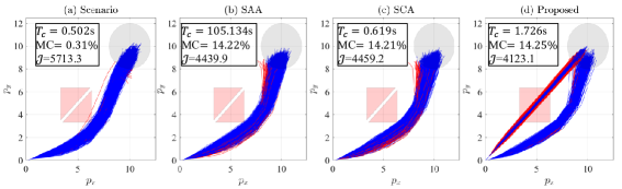
Figure 3: Solutions from different methods for the tolerable failure probability threshold $\alpha=15\%$. Blue trajectories from Monte-Carlo (MC) simulations denote feasible trajectories that reach the goal set $\mathcal{S}_{goal}$ and avoid obstacles $\mathcal{O}$. Red trajectories mean that either constraint is violated in the simulation. The expression $\mathsf{MC}=14.22\%$ means the probability of having red trajectories in the MC simulations. (a) Scenario; (b) SAA; (c) SCA; (d) Proposed.

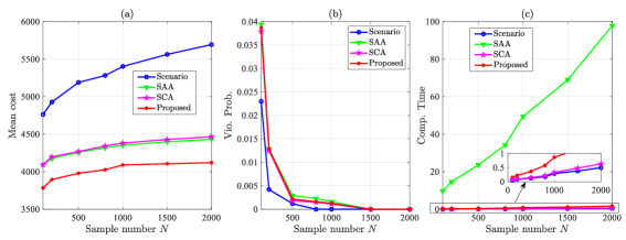
Figure 4: Plot of the results in Table I. (a) $\mathbb{E}\{\mathcal{J}\}$; (b) $\mathbb{\mathsf{Pr}}\{\alpha>0.15\}\}$; (c) $\mathbb{E}\{T_{c}\}$.

Results of one specific case are shown in Fig. 3 for four different methods by setting $\alpha$ as $15\%$, the number of $\omega_{t}$ samples as $2000$ for all four methods. Besides, the parameters $\varepsilon$ and $\gamma$ are both $0.01$ for SCA and Proposed. Fig. 3 shows $10,000$ Monte-Carlo (MC) simulations of the quadrotor system using the open-loop policies computed by four different methods. The deterministic decision generated by Scenario leads to a very safe trajectory with only $0.31\%$ in the MC simulations. However, the expected cost $\mathcal{J}$ is high. Scenario is originally developed for robust optimization and thus gives a much more conservative solution than the required violation probability threshold. The deterministic control policies generated by SAA, and SCA give almost the same trajectories which optimize the cost $\mathcal{J}$ much more than Scenario and still satisfy the required chance constraint. Since a mixed integer program needs to be solved in SAA, the computation time $T_{c}$ is much longer than SCA and Scenario. When the probabilistic decision generated by Proposed is implemented, the cost $\mathcal{J}$ is further improved with some sacrifice in the computation time while keeping the risk at the same level. This shows that stochastic policies can improve the expectations of the objective function.

A more comprehensive statistical analysis has been implemented by conducting the Monter-Carlo trials 1000 times when the parameters in the simulation are fixed. In each Monter-Carlo trial, $10,000$ Monte-Carlo (MC) simulations of the quadrotor system are implemented to calculate the violation probability and the expected cost. In this validation, the sample number of $\alpha^{(i)}$ is set as 50 for Proposed. The results are summarized in Table I and are plotted in Figure 4 for visualization.

The deterministic policy obtained by Scenario shows high robustness to uncertainties but also costs more. Note that the deterministic decision obtained by Scenario corresponds to the completely robust decision, which cannot be improved if complete robustness is required. However, in our setting, we allow a probability of risk as $15\%$, and it is possible to obtain better performance using measurable policy. The measurable policy obtained by Proposed sacrifices some computation time to obtain a better mean objective function satisfying the chance constraint. The above observations are the same as the examples in Figure 3.

The computation time of the proposed method is still too high for implementation in implicit MPC in real-time applications. However, we could embed the proposed method in explicit MPC, in which the policy is calculated offline, and then apply the calculated policy online. Regarding the violation probability, even with 100 samples, the probability of violating the chance constraints is very low for all methods. Besides, Table I shows that the sample number of $\xi$ is a key factor of the computational time. For future work, we will work on how to improve the computation efficiency by reducing sample size. A sample-free method for solving chance-constrained optimization is also a possible way.

In this paper, we give a trajectory planning and control problem to show that the proposed probabilistic decision method outperforms the existing deterministic decision methods. It is effective not only for trajectory planning and control problems. Applications for planning problems with uncertainties can also be addressed by the proposed probabilistic decision method, including optimal economic dispatch with renewable energy generation, such as photovoltaic power generation and wind power generation. We leave the extensions of our method for future work.

7 Conclusions and Future Work

In a probabilistic decision-making problem under chance constraint, decision variables are probabilistically chosen to optimize the expected objective value under chance constraint. We formulate the probabilistic decision-making problem under chance constraints as the chance-constrained probability measure optimization. We prove the existence of the optimal solution to the chance-constrained probability measure optimization. Furthermore, we show that there exists an optimal solution that the probability measure is concentrated on two decisions. Then, an equivalent reduced problem of the chance-constrained probability measure optimization is established. The sample-based smooth approximation method has been extended to solve the reduced problem. The analysis of uniform convergence and feasibility is given. A numerical example of a quadrotor system control problem has been implemented to validate the performance of the proposed probabilistic decision-making under chance constraints. Future work will be focused on implementing the proposed method to design optimal feedback probabilistic control policy with the satisfaction of the chance constraints.

Appendix A Proof of Theorem 2

For $S\in\mathbb{N}$, let $\left(\mu_{S},\mathcal{C}_{S}\right)\in\tilde{\mathcal{U}}_{\alpha}(S)$ be a feasible solution to Problem $\tilde{P}_{\alpha}(S)$ with $\mathcal{C}_{S}=\left(x^{(1)},...,x^{(i)},...,x^{(S)}\right)$. Let $\mu_{S}^{\mathsf{m}}\in M(\mathcal{X})$ be a measure that satisfies $\mu_{S}^{\mathsf{m}}\left(\{x^{(i)}\}\right)=\mu_{S}(i),i\in[S]$. We have

$$\int_{\mathcal{X}}\mathbb{P}(x)\mathsf{d}\mu_{S}^{\mathsf{m}}(x)=\sum_{i=1}^{S}\mathbb{P}(x^{(i)})\mu_{S}(i)\geq 1-\alpha,$$ (47)

which implies that $\mu_{S}^{\mathsf{m}}\in M_{\alpha}(x)$, where $M_{\alpha}(x)$ is the feasible solution set of Problem $P_{\alpha}$ defined by (16). Then, for all $\left(\mu_{S},\mathcal{C}_{S}\right)\in\tilde{\mathcal{U}}_{\alpha}(S),$ $S\in\mathbb{N}$, it holds that

$$\sum_{i=1}^{S}J(x^{(i)})\mu_{S}(i)=\int_{\mathcal{X}}J(x)\mathsf{d}\mu_{S}^{\mathsf{m}}(x)\geq\mathcal{J}^{*}_{\alpha},$$ (48)

which implies $\tilde{\mathcal{J}}_{\alpha}(S)\geq\mathcal{J}^{*}_{\alpha},$ for all $S\in\mathbb{N}$, and consequently we have

$$\liminf_{S\rightarrow\infty}\tilde{\mathcal{J}}_{\alpha}(S)\geq\mathcal{J}^{*}_{\alpha}.$$ (49)

Assumption 2 implies that there exists a sequence $\{\mu_{k}\}_{k=1}^{\infty}\subseteq M(\mathcal{X})$ that converges to an optimal solution $\mu^{*}$ of Problem $P_{\alpha}$ associated with $J$, such that

$$\int_{\mathcal{X}}\mathbb{P}(x)\mathsf{d}\mu_{k}>1-\alpha,~{}~{}\forall k\geq 1.$$ (50)

For any given $\varepsilon>0$, by the definition of convergence associated with $J$ (Definition 1), there exists $k_{\varepsilon}$ such that, if $k\geq k_{\varepsilon}$,

$$0\leq\int_{\mathcal{X}}J(x)\mathsf{d}\mu_{k}(x)-\mathcal{J}^{*}_{\alpha}\leq\frac{\varepsilon}{2},$$ (51)

since $\mu^{*}$ is an optimal solution of Problem $P_{\alpha}$, i.e., $\mathcal{J}^{*}_{\alpha}=\int_{\mathcal{X}}J(x)\mathsf{d}\mu^{*}$ by (17).

Let ${\mathcal{C}}_{{S}}^{k_{\varepsilon}}:=\{x^{(1)}_{k_{\varepsilon}},...,x^{(S)}_{k_{\varepsilon}}\},S\in\mathbb{N},$ be a sample set obtained by sampling from $\mathcal{X}$ according to probability measure $\mu_{k_{\varepsilon}}$. By Law of Large Numbers (p. 457 of [12]), for any continuous function $f\in\mathscr{C}(\mathcal{X})$, as $S\rightarrow\infty$, w.p.1, we have

$$\frac{1}{S}\sum_{i=1}^{S}f(x^{(i)}_{k_{\varepsilon}})\rightarrow\mathbb{E}_{x\sim\mu_{k_{\varepsilon}}}\left\{f(x)\right\}=\int_{\mathcal{X}}f(x)\mathsf{d}\mu_{k_{\varepsilon}}.$$ (52)

Notice that $J(\cdot)$ and $\mathbb{P}(\cdot)$ are continuous. Then, (52) also holds by replacing $f(\cdot)$ by either $J(\cdot)$ or $\mathbb{P}(\cdot)$. As a result, for given

$$\varepsilon_{1}=\min\left\{\frac{\varepsilon}{2},\int_{\mathcal{X}}\mathbb{P}(x)\mathsf{d}\mu_{k_{\varepsilon}}-(1-\alpha)\right\}>0,$$ (53)

there exists $S(\varepsilon)=S(\varepsilon,k_{\varepsilon})$ such that, if $S\geq S(\varepsilon)$, w.p.1, the followings hold:

$$\left|\frac{1}{S}\sum_{i=1}^{S}\mathbb{P}({x}^{(i)}_{{k_{\varepsilon}}})-\int_{\mathcal{X}}\mathbb{P}(x)\mathsf{d}\mu_{k_{\varepsilon}}\right|\leq\varepsilon_{1},$$ (54)

$$\left|\frac{1}{S}\sum_{i=1}^{S}J(\tilde{x}^{(i)}_{k_{\varepsilon}})-\int_{\mathcal{X}}J(x)\mathsf{d}\mu_{k_{\varepsilon}}\right|\leq\varepsilon_{1},$$ (55)

for sample set ${\mathcal{C}}_{{S}}^{k_{\varepsilon}}.$ Define a discrete probability measure $\mu^{S}_{k}\in M(\mathcal{X}),S\geq S(\varepsilon)$ such that

$$\mu_{S}^{k_{\varepsilon}}(i)=\frac{1}{S},\ \forall i\in[S],$$ (56)

where $\mu_{S}^{k_{\varepsilon}}(i)$ is the discrete probability assigned to ${x}^{(i)}_{k_{\varepsilon}}$, i.e., $\mu_{S}^{k_{\varepsilon}}({x}^{(i)}_{k_{\varepsilon}})=\mu_{S}^{k_{\varepsilon}}(i)$. Then, from (53), and (54), we have

$$\sum_{i=1}^{S}\mathbb{P}({x}^{(i)}_{k_{\varepsilon}})\mu_{S}^{k_{\varepsilon}}(i)\geq\int_{\mathcal{X}}\mathbb{P}(x)\mathsf{d}\mu_{k_{\varepsilon}}-{\varepsilon}_{1}\geq 1-\alpha,$$ (57)

which implies for each $S\geq S(\varepsilon)$, w.p.1, $\left(\mu_{S}^{k_{\varepsilon}},{\mathcal{C}}^{k_{\varepsilon}}_{S}\right)$ is a feasible solution of Problem $\tilde{P}_{\alpha}(S)$ and thus

$$\sum_{i=1}^{S}J({x}_{k_{\varepsilon}}^{(i)})\mu_{S}^{k_{\varepsilon}}(i)\geq\tilde{\mathcal{J}}_{\alpha}(S),~{}~{}~{}w.p.1.$$ (58)

Considering (55) and (58), we have

$$\tilde{\mathcal{J}}_{\alpha}(S)-\int_{\mathcal{X}}J(x)\mathsf{d}\mu^{k_{\varepsilon}}\leq\tilde{\varepsilon}_{1}.$$ (59)

For $S\geq S(\varepsilon)$, combining (51) and (59), we have

$$\tilde{\mathcal{J}}_{\alpha}(S)-\mathcal{J}^{*}_{\alpha}\leq\frac{\varepsilon}{2}+\varepsilon_{1}\leq\varepsilon,$$ (60)

which implies $\limsup_{S\rightarrow\infty}\tilde{\mathcal{J}}_{\alpha}(S)\leq\mathcal{J}^{*}_{\alpha}+\varepsilon$. Finally, by arbitrary of $\varepsilon$, we have

$$\limsup_{S\rightarrow\infty}\tilde{\mathcal{J}}_{\alpha}(S)\leq\mathcal{J}^{*}_{\alpha}.$$ (61)

With (49) and (61), we proof that (26).

Appendix B Proof of Corollary 1

Suppose that $x^{(1)}_{*}\notin X_{\tilde{\alpha}^{(1)}}$. Then, $J(x^{(1)}_{*})>J^{*}_{\tilde{\alpha}^{(1)}}$ holds. Let $\hat{x}^{(1)}\in X_{\tilde{\alpha}^{(1)}}$. Then, $\mathbb{P}(\hat{x}^{(1)})\geq 1-\tilde{\alpha}^{(1)}=\mathbb{P}(x^{(1)}_{*})$ and $J(\hat{x}^{(1)})=J^{*}_{\tilde{\alpha}^{(1)}}<J(x^{(1)}_{*})$. We have

$$\displaystyle\mathbb{P}(\hat{x}^{(1)})\mu^{*}_{\mathsf{m}}(1)+\mathbb{P}(x^{(2)}_{*})\mu^{*}_{\mathsf{m}}(2)\geq\sum_{i=1}^{2}\mathbb{P}(x^{(i)}_{*})\mu^{*}_{\mathsf{m}}(i)\geq 1-\alpha,$$

$$\displaystyle J(\hat{x}^{(1)})\mu^{*}_{\mathsf{m}}(1)+J(x^{(2)}_{*})\mu^{*}_{\mathsf{m}}(2)<\sum_{i=1}^{2}J(x^{(i)}_{*})\mu^{*}_{\mathsf{m}}(i).$$

Thus, $\hat{\bm{z}}_{\mathsf{m}}=\left(\mu_{\mathsf{m}}^{*}(1),\mu_{\mathsf{m}}^{*}(2),\hat{x}^{(1)},x^{(2)}_{*}\right)$ is a feasible solution of $W_{\alpha}$ and has a smaller objective function value than $\bm{z}_{\mathsf{m}}^{*}$ which contradicts to $\bm{z}_{\mathsf{m}}^{*}\in D_{\alpha}$. Therefore, we have $x^{(1)}_{*}\in X_{\tilde{\alpha}^{(1)}}$. Follow the above procedures, we could also prove that $x^{(2)}_{*}\in X_{\tilde{\alpha}^{(2)}}$.

Appendix C Proof of Corollary 2

Let $\bm{z}_{\mathsf{m}}^{*}=\left(\mu_{\mathsf{m}}^{*}(1),\mu_{\mathsf{m}}^{*}(2),x^{(1)}_{*},x^{(2)}_{*}\right)\in D_{\alpha}$ be an optimal solution of Problem $W_{\alpha}$. Let $\tilde{\alpha}^{(1)}=1-\mathbb{P}(x^{(1)}_{*})$ and $\tilde{\alpha}^{(2)}=1-\mathbb{P}(x^{(2)}_{*})$. By Corollary 1, we have $J(x^{(1)}_{*})=J^{*}_{\tilde{\alpha}^{(1)}}$ and $J(x^{(2)}_{*})=J^{*}_{\tilde{\alpha}^{(2)}}$. Without loss of generality, suppose $\tilde{\alpha}^{(1)}<\tilde{\alpha}^{(2)}$. Let $\tilde{\alpha}^{\mathsf{com}}:=\mu_{\mathsf{m}}^{*}(1)\tilde{\alpha}^{(1)}+\mu_{\mathsf{m}}^{*}(2)\tilde{\alpha}^{(2)}$. Note that $\tilde{\alpha}^{\mathsf{com}}\leq\alpha$ since $\bm{z}_{\mathsf{m}}^{*}$ is feasible for $W_{\alpha}$. Because $J^{*}_{\tilde{\alpha}}$ is a convex function of $\tilde{\alpha}$, we have

$$J^{*}_{\tilde{\alpha}^{\mathsf{com}}}\leq J^{*}_{\tilde{\alpha}^{(1)}}\mu_{\mathsf{m}}^{*}(1)+J^{*}_{\tilde{\alpha}^{(2)}}\mu_{\mathsf{m}}^{*}(2)=\mathcal{J}^{*}_{\alpha}.$$ (62)

The last equality holds due to Theorem 3. Since $J^{*}_{\tilde{\alpha}}$ is monotonically decreasing function of $\tilde{\alpha}$, we have

$$J^{*}_{\alpha}\leq J^{*}_{\tilde{\alpha}^{\mathsf{com}}}\leq\mathcal{J}^{*}_{\alpha}.$$ (63)

By (21) and (22), $J^{*}_{\alpha}\geq\mathcal{J}^{*}_{\alpha}$ holds. Thus, $\mathcal{J}^{*}_{\alpha}=J^{*}_{\alpha}$ holds.

If $\alpha=0$, $\tilde{\alpha}^{(1)}=\tilde{\alpha}^{(2)}$ must holds when both $\mu^{*}_{\mathsf{m}}(1)$ and $\mu^{*}_{\mathsf{m}}(2)$ are positive. Then, $J(x^{(1)}_{*})=J(x^{(2)}_{*})=J^{*}_{0}$ since $x^{(1)}_{*},x^{(2)}_{*}\in X_{0}$. Thus, $\mathcal{J}_{0}^{*}=\left(\mu_{\mathsf{m}}^{*}(1)+\mu_{\mathsf{m}}^{*}(2)\right)J^{*}_{0}=J^{*}_{0}$.

Appendix D Proof of Proposition 2

For an arbitrary $S\in\mathbb{N}$, let $\left(\tilde{\mu}_{\alpha},\tilde{\mathcal{C}}_{S}\right)\in\tilde{A}_{\alpha}(S)$ be an optimal solution of Problem $\tilde{P}_{\alpha}(S)$, where $\tilde{\mathcal{C}}_{S}=\left(x^{(1)},...,x^{(i)},...,x^{(S)}\right)$. Notice that $\tilde{\mu}_{\alpha}(i)$ is the discrete probability assigned to $x^{(i)}$ for $i\in[S]$. We have that

$$\sum_{i=1}^{S}J(x^{(i)})\tilde{\mu}_{\alpha}(i)=\tilde{\mathcal{J}}_{\alpha}(S),$$ (64)

$$\sum_{i=1}^{S}\mathbb{P}(x^{(i)})\tilde{\mu}_{\alpha}(i)\geq 1-\alpha.$$ (65)

Define a set of violation probabilities as

$$\mathcal{E}_{S}=\left(\tilde{\alpha}^{(1)},...,\tilde{\alpha}^{(S)}\right),$$ (66)

where $\tilde{\alpha}^{(i)}=1-\mathbb{P}(x^{(i)})$. Let $\nu_{S}\in\mathcal{V}_{S}$ be a probability measure that satisfies $\nu_{S}(i)=\tilde{\mu}_{\alpha}(i),i\in[S]$. Then, $\bm{\theta}_{S}=\{\nu_{S},\mathcal{E}_{S}\}$ is a feasible solution of Problem $\tilde{V}_{\alpha}(S)$ since

$$\sum_{i=1}^{S}(1-\tilde{\alpha}^{(i)})\nu_{S}(i)=\sum_{i=1}^{S}\mathbb{P}(x^{(i)})\tilde{\mu}_{\alpha}(i)\geq 1-\alpha.$$ (67)

Besides, we have

$$\sum_{i=1}^{S}J^{*}_{\tilde{\alpha}^{(i)}}\nu_{S}(i)\leq\sum_{i=1}^{S}J(x^{(i)})\tilde{\mu}_{\alpha}(i)=\tilde{\mathcal{J}}_{\alpha}(S).$$ (68)

To show $\sum_{i=1}^{S}J^{*}_{\tilde{\alpha}^{(i)}}\nu_{S}(i)=\tilde{\mathcal{J}}_{\alpha}(S)$, we need to prove that $\sum_{i=1}^{S}J^{*}_{\tilde{\alpha}^{(i)}}\nu_{S}(i)\geq\tilde{\mathcal{J}}_{\alpha}(S)$ also holds.

For $\mathcal{E}_{S}$ defined by (66), define a set of decision variables as $\hat{\mathcal{C}}_{S}=\{\hat{x}^{(i)}\}_{i=1}^{S}$, where $\hat{x}^{(i)}\in X_{\tilde{\alpha}^{(i)}}$ is an optimal solution of Problem $Q_{\tilde{\alpha}^{(i)}}$. Notice that we have $\mathbb{P}(\hat{x}^{(i)})\geq 1-\tilde{\alpha}^{(i)}$ and $J(\hat{x}^{(i)})=J^{*}_{\tilde{\alpha}^{(i)}}$. Let $\hat{\mu}_{S}(i)=\nu_{S}(i)$ and $\left(\hat{\mu}_{S},\hat{C}_{S}\right)$ is then a feasible solution of Problem $\tilde{P}_{\alpha}(S)$ since we have

$$\sum_{i=1}^{S}\mathbb{P}(\hat{x}^{(i)})\hat{\mu}_{S}(i)\geq\sum_{i=1}^{S}(1-\tilde{\alpha}^{(i)})\nu_{S}(i)\geq 1-\alpha.$$ (69)

Therefore, we have

$$\sum_{i=1}^{S}J^{*}_{\tilde{\alpha}^{(i)}}\nu_{S}(i)=\sum_{i=1}^{S}J(\hat{x}^{(i)})\hat{\mu}_{S}(i)\geq\tilde{\mathcal{J}}_{\alpha}(S)$$ (70)

By (68) and (70), we have (32).

Appendix E Proof of Lemma 1

Define a set $\mathcal{H}:=[0,1]\times\mathbb{R}$. Let $(\tilde{\alpha},J^{*}_{\tilde{\alpha}})\in\mathcal{H}$ be a pair of violation probability threshold $\tilde{\alpha}$ and the corresponding optimal objective value of $Q_{\tilde{\alpha}}$. Let $\mathsf{conv}(\mathcal{H})$ be the convex hull of $\mathcal{H}$.

Construct a new optimization problem as

$$\begin{split}&\underset{(\tilde{\alpha}_{\mathsf{h},\alpha},J_{\mathsf{h}})\in\mathsf{conv}(\mathcal{H})}{{\mathsf{min}}}\,\,J_{\mathsf{h}}\\ &{\mathsf{s.t.}}\quad 1-\tilde{\alpha}_{\mathsf{h},\alpha}\geq 1-\alpha.\end{split} H_{\alpha}$$ ()

Let $(\tilde{\alpha}_{\mathsf{h},\alpha}^{\diamond},J^{\diamond}_{\mathsf{h},\alpha})$ be an optimal solution of Problem $H_{\alpha}$.

We first show that $J^{\diamond}_{\mathsf{h},\alpha}\leq\mathcal{J}^{*}_{\alpha}$ holds, for any $S\in N$. Let $\bm{\theta}_{S}:=\{\nu_{S},\tilde{\alpha}^{(1)},...,\tilde{\alpha}^{(S)}\}$ be a feasible solution of Problem $\tilde{V}_{\alpha}(S)$ that satisfies (32) in Proposition 2. Note that $\mathcal{E}_{S}:=\{\tilde{\alpha}^{(1)},...,\tilde{\alpha}^{(S)}\}$ is a sample set of violation probabilities. Define a point $\left(\tilde{\alpha}_{\mathsf{mean}}(\bm{\theta}_{S}),J^{*}_{\mathsf{mean}}(\bm{\theta}_{S})\right)\in\mathsf{conv}(\mathcal{H})$ by

$$\tilde{\alpha}_{\mathsf{mean}}(\bm{\theta}_{S}):=\sum_{i=1}^{S}\tilde{\alpha}^{(i)}\nu_{S}(i),$$ (71)

$$J^{*}_{\mathsf{mean}}(\bm{\theta}_{S}):=\sum_{i=1}^{S}J^{*}_{\tilde{\alpha}^{(i)}}\nu_{S}(i).$$ (72)

By the definition of convex hull, we have the point $\left(\tilde{\alpha}_{\mathsf{mean}}(\bm{\theta}_{S}),J^{*}_{\mathsf{mean}}(\bm{\theta}_{S})\right)\in\mathsf{conv}(\mathcal{H})$. Since $\bm{\theta}_{S}$ is a feasible optimal solution, we have $1-\tilde{\alpha}_{\mathsf{mean}}(\bm{\theta}_{S})\geq 1-\alpha$ and $J^{*}_{\mathsf{mean}}(\bm{\theta}_{S})=\tilde{\mathcal{J}}_{\alpha}(S)$ by Proposition 2. Thus, for all $S\in\mathbb{N}$, $\left(\tilde{\alpha}_{\mathsf{mean}}(\bm{\theta}_{S}),J^{*}_{\mathsf{mean}}(\bm{\theta}_{S})\right)$ is a feasible point of problem $H_{\alpha}$ and we have

$$J^{\diamond}_{\mathsf{h},\alpha}\leq\tilde{\mathcal{J}}_{\alpha}(S).$$ (73)

Notice that (73) implies that $J^{\diamond}_{\mathsf{h},\alpha}\leq\lim_{S\rightarrow\infty}\tilde{\mathcal{J}}_{\alpha}(S)$. Then, by Theorem 2, we have

$$J^{\diamond}_{\mathsf{h},\alpha}\leq\mathcal{J}^{*}_{\alpha}.$$ (74)

Next, we show that $(\tilde{\alpha}_{\mathsf{h},\alpha}^{\diamond},J^{\diamond}_{\mathsf{h},\alpha})$ is one boundary point of $\mathsf{conv}(\mathcal{H})$. Suppose on the contrary that $(\tilde{\alpha}_{\mathsf{h},\alpha}^{\diamond},J^{\diamond}_{\mathsf{h},\alpha})$ is an interior point. Thus there exists a neighborhood of $(\tilde{\alpha}_{\mathsf{h},\alpha}^{\diamond},J^{\diamond}_{\mathsf{h},\alpha})$ such that is within $\mathsf{conv}(\mathcal{H})$. Suppose that $\mathcal{B}_{\varepsilon}\left((\tilde{\alpha}_{\mathsf{h},\alpha}^{\diamond},J^{\diamond}_{\mathsf{h},\alpha})\right)\subset\mathsf{conv}(\mathcal{H})$, where $\varepsilon>0$. For any $\tilde{\varepsilon}<\varepsilon$, we have that $(\tilde{\alpha}_{\mathsf{h},\alpha}^{\diamond},J^{\diamond}_{\mathsf{h},\alpha}-\tilde{\epsilon})\in\mathcal{B}_{\varepsilon}\left((\tilde{\alpha}_{\mathsf{h},\alpha}^{\diamond},J^{\diamond}_{\mathsf{h},\alpha})\right)\subset\mathsf{conv}(\mathcal{H})$. Since $1-\tilde{\alpha}_{\mathsf{h},\alpha}^{\diamond}\geq 1-\alpha$, $(\tilde{\alpha}_{\mathsf{h},\alpha}^{\diamond},J^{\diamond}_{\mathsf{h},\alpha}-\tilde{\epsilon})$ is a feasible solution of $H_{\alpha}$. However, $J^{\diamond}_{\mathsf{h},\alpha}-\tilde{\epsilon}<J^{\diamond}_{\mathsf{h},\alpha}$ holds and it contracts with that $(\tilde{\alpha}_{\mathsf{h},\alpha}^{\diamond},J^{\diamond}_{\mathsf{h},\alpha})$ is an optimal solution of $H_{\alpha}$. Thus, $(\tilde{\alpha}_{\mathsf{h},\alpha}^{\diamond},J^{\diamond}_{\mathsf{h},\alpha})$ is a boundary point.

By supporting hyperplane theorem (p. 133 of [36]), there exists a line $\mathcal{L}$ that passes through the boundary point $(\tilde{\alpha}_{\mathsf{h},\alpha}^{\diamond},J^{\diamond}_{\mathsf{h}})$ and contains $\mathsf{conv}(\mathcal{H})$ in one of its closed half-spaces. Note that $\mathcal{L}$ is a one-dimensional linear space. Therefore, we can also say $(\tilde{\alpha}_{\mathsf{h},\alpha}^{\diamond},J^{\diamond}_{\mathsf{h}})$ is within the convex hull of $\mathcal{L}\bigcap\mathcal{H}$, $\mathsf{conv}(\mathcal{L}\bigcap\mathcal{H})$, namely, $(\tilde{\alpha}_{\mathsf{h},\alpha}^{\diamond},J^{\diamond}_{\mathsf{h}})\in\mathsf{conv}(\mathcal{L}\bigcap\mathcal{H})$. By Caratheodory’s theorem [37], we have that $(\tilde{\alpha}_{\mathsf{h},\alpha}^{\diamond},J^{\diamond}_{\mathsf{h}})\in\mathsf{conv}(\mathcal{L}\bigcap\mathcal{H})$ is within the convex combination of at most two points in $\mathcal{L}\bigcap\mathcal{H}$, namely, $\exists\nu_{\mathsf{m}}^{\diamond}\in\mathcal{V}_{2},\ \exists\{\tilde{\alpha}^{(1)}_{\mathsf{m}},\tilde{\alpha}^{(2)}_{\mathsf{m}}\}\in[0,1]^{2}$ such that $J^{\diamond}_{\mathsf{h},\alpha}=J^{*}_{\tilde{\alpha}^{(1)}_{\mathsf{m}}}\nu^{\diamond}_{\mathsf{m}}(1)+J^{*}_{\tilde{\alpha}^{(2)}_{\mathsf{m}}}\nu^{\diamond}_{\mathsf{m}}(2)$ and $\tilde{\alpha}_{\mathsf{h},\alpha}^{\diamond}=\tilde{\alpha}^{(1)}_{\mathsf{m}}\nu^{\diamond}_{\mathsf{m}}(1)+\tilde{\alpha}^{(2)}_{\mathsf{m}}\nu^{\diamond}_{\mathsf{m}}(2)$. It holds that

$$1-\left(\tilde{\alpha}^{(1)}_{\mathsf{m}}\nu^{\diamond}_{\mathsf{m}}(1)+\tilde{\alpha}^{(2)}_{\mathsf{m}}\nu^{\diamond}_{\mathsf{m}}(2)\right)=1-\tilde{\alpha}_{\mathsf{h},\alpha}^{\diamond}\geq 1-\alpha.$$

Thus, $\left(\nu^{\diamond}_{\mathsf{m}}(1),\nu^{\diamond}_{\mathsf{m}}(2),\tilde{\alpha}_{\mathsf{m}}^{(1)},\tilde{\alpha}_{\mathsf{m}}^{(2)}\right)$ is a feasible solution of Problem $\tilde{V}_{\alpha}(S)$ when $S=2$. Let $\tilde{x}_{\mathsf{m}}^{(1)}\in X_{\tilde{\alpha}_{\mathsf{m}}^{(1)}}$ and $\tilde{x}_{\mathsf{m}}^{(2)}\in X_{\tilde{\alpha}_{\mathsf{m}}^{(2)}}$ be the optimal solutions of Problems $Q_{\tilde{\alpha}_{\mathsf{m}}^{(1)}}$ and $Q_{\tilde{\alpha}_{\mathsf{m}}^{(2)}}$. Then, we have $J(\tilde{x}_{\mathsf{m}}^{(1)})=J^{*}_{\tilde{\alpha}_{\mathsf{m}}^{(1)}}$, $J(\tilde{x}_{\mathsf{m}}^{(2)})=J^{*}_{\tilde{\alpha}_{\mathsf{m}}^{(2)}}$, $\mathbb{P}(\tilde{x}_{\mathsf{m}}^{(1)})=1-\tilde{\alpha}_{\mathsf{m}}^{(1)}$, and $\mathbb{P}(\tilde{x}_{\mathsf{m}}^{(2)})=1-\tilde{\alpha}_{\mathsf{m}}^{(2)}$. By repeating (69), we have that $\left(\nu^{\diamond}_{\mathsf{m}}(1),\nu^{\diamond}_{\mathsf{m}}(2),\tilde{x}_{\mathsf{m}}^{(1)},\tilde{x}_{\mathsf{m}}^{(2)}\right)$ is a feasible solution of Problem $\tilde{P}_{\alpha}(S)$ when $S=2$. Thus, we have

$$J^{\diamond}_{\mathsf{h},\alpha}=\sum_{i=1}^{2}J(\tilde{x}_{\mathsf{m}}^{(i)})\nu^{\diamond}_{\mathsf{m}}(i)\geq\tilde{\mathcal{J}}_{\alpha}(2)\geq\mathcal{J}^{*}_{\alpha}.$$ (75)

By (74) and (75), we have $J^{*}_{\tilde{\alpha}^{(1)}_{\mathsf{m}}}\nu^{\diamond}_{\mathsf{m}}(1)+J^{*}_{\tilde{\alpha}^{(2)}_{\mathsf{m}}}\nu^{\diamond}_{\mathsf{m}}(2)=J^{\diamond}_{\mathsf{h},\alpha}=\mathcal{J}^{*}_{\alpha}$, which implies (33).

Appendix F Proof of Theorem 4

By Assumption 3, the set $X_{\tilde{\alpha}}$ is not empty for any $\tilde{\alpha}\in[0,1]$ and there exists $x\in\mathcal{X}$ such that $\mathbb{P}(x)>1-\tilde{\alpha}$. By Theorem 3.4 of [20], $\tilde{\mathbb{P}}_{N}^{\gamma,\varepsilon}(x)$ converges to $\mathbb{P}(x)$ as $N\rightarrow\infty$, thus, there exists $\varepsilon_{0}$ small enough and $N_{0}$ large enough such that $\tilde{\mathbb{P}}_{N}^{\gamma,\varepsilon}(x)\geq 1-\tilde{\alpha},$ for any $N>N_{0}$ w.p.1. Notice that $\tilde{\mathbb{P}}_{N}^{\gamma,\varepsilon}(x)$ is continuous in $x$ and $\mathcal{X}$ is compact, and then the feasible set of Problem $\tilde{W}_{\tilde{\alpha}}^{\gamma,\varepsilon}(\mathcal{D}_{N})$ is compact. Thus, $\tilde{X}_{\tilde{\alpha}}^{\gamma,\varepsilon}$ is nonempty for all $N\geq N_{0}$ and $\varepsilon\leq\varepsilon_{0}$.

Define two sequences $\{N_{k}\}_{k=1}^{\infty}\geq N_{0}$ and $\{\varepsilon_{k}\}_{k=1}^{\infty}$, where $N_{k}\rightarrow\infty$ and $\varepsilon_{k}\rightarrow 0$. For each $N_{k}$ and $\varepsilon_{k}$, there exists a corresponding optimal solution $\tilde{\bm{z}}_{\mathsf{m},\alpha}^{\gamma,\varepsilon_{k}}(\mathcal{D}_{N_{k}})\in\tilde{D}_{\alpha}^{\gamma,\varepsilon_{k}}(\mathcal{D}_{N_{k}})$ of Problem $\tilde{W}^{\gamma,\varepsilon_{k}}_{\alpha}(\mathcal{D}_{N_{k}})$, which is represented by $\tilde{\bm{z}}_{\mathsf{m},\alpha}^{k}$ in this proof for simplicity. Then, we have a sequence $\{\tilde{\bm{z}}^{k}_{\mathsf{m},\alpha}\}_{k=1}^{\infty}$. Specify the components of $\tilde{\bm{z}}_{\mathsf{m},\alpha}^{k}$ by $\tilde{\bm{z}}^{k}_{\mathsf{m},\alpha}=\left(\tilde{\mu}_{\mathsf{m}}^{k}(1),\tilde{\mu}_{\mathsf{m}}^{k}(2),\tilde{x}^{(1)}_{k},\tilde{x}^{(2)}_{k}\right)$. Let $\tilde{\alpha}_{\mathsf{sca},k}^{(1)}=1-\tilde{\mathbb{P}}^{\gamma,\varepsilon_{k}}_{N_{k}}(\tilde{x}_{k}^{(1)})$ and $\tilde{\alpha}_{\mathsf{sca},k}^{(2)}=1-\tilde{\mathbb{P}}^{\gamma,\varepsilon_{k}}_{N_{k}}(\tilde{x}_{k}^{(2)})$ be sample-based smooth approximation of the violation probability. By repeating the proof of Corollary 1, we can obtain that $\tilde{x}_{k}^{(1)}\in\tilde{X}_{\tilde{\alpha}_{\mathsf{sca},k}^{(1)}}^{\gamma,\varepsilon_{k}}(\mathcal{D}_{N_{k}})$ and $\tilde{x}_{k}^{(2)}\in\tilde{X}_{\tilde{\alpha}_{\mathsf{sca},k}^{(2)}}^{\gamma,\varepsilon_{k}}(\mathcal{D}_{N_{k}})$. Thus, $J(\tilde{x}_{k}^{(1)})=\tilde{J}^{\gamma,\varepsilon_{k}}_{\tilde{\alpha}_{\mathsf{sca},k}^{(1)}}(\mathcal{D}_{N_{k}})$ and $J(\tilde{x}_{k}^{(2)})=\tilde{J}^{\gamma,\varepsilon_{k}}_{\tilde{\alpha}_{\mathsf{sca},k}^{(2)}}(\mathcal{D}_{N_{k}})$. For every $k$, we have

$$\tilde{\mathbb{P}}^{\gamma,\varepsilon_{k}}_{N_{k}}(\tilde{x}_{k}^{(1)})\tilde{\mu}_{\mathsf{m}}^{k}(1)+\tilde{\mathbb{P}}^{\gamma,\varepsilon_{k}}_{N_{k}}(\tilde{x}_{k}^{(2)})\tilde{\mu}_{\mathsf{m}}^{k}(2)\geq 1-\alpha.$$ (76)

Let $\tilde{\bm{z}}^{\mathsf{lim}}_{\mathsf{m},\alpha}=\left(\tilde{\mu}_{\mathsf{m}}^{\mathsf{lim}}(1),\tilde{\mu}_{\mathsf{m}}^{\mathsf{lim}}(2),\tilde{x}^{(1)}_{\mathsf{lim}},\tilde{x}^{(2)}_{\mathsf{lim}}\right)$ be an arbitrary cluster point of $\{\tilde{\bm{z}}^{k}_{\mathsf{m},\alpha}\}_{k=1}^{\infty}$ and $\{\tilde{\bm{z}}^{l}_{\mathsf{m},\alpha}\}_{l=1}^{\infty}$ be a subsequence that converges to $\tilde{\bm{z}}^{\mathsf{lim}}_{\mathsf{m},\alpha}$. Because $\tilde{\mathbb{P}}^{\gamma,\varepsilon_{l}}_{N_{l}}(x)$ converges uniformly to $\mathbb{P}(x)$ on $\mathcal{X}$ w.p.1 by Theorem 3.4 of [20], we have

$$\mathbb{P}(\tilde{x}_{\mathsf{lim}}^{(1)}) = \lim_{l\rightarrow\infty}\tilde{\mathbb{P}}^{\gamma,\varepsilon_{l}}_{N_{l}}(\tilde{x}_{k}^{(1)})=\tilde{\mathbb{P}}^{\gamma,\varepsilon_{\mathsf{lim}}}_{N_{\mathsf{lim}}}(\tilde{x}_{\mathsf{lim}}^{(1)}),$$ (77)

$$\mathbb{P}(\tilde{x}_{\mathsf{lim}}^{(2)}) = \lim_{l\rightarrow\infty}\tilde{\mathbb{P}}^{\gamma,\varepsilon_{l}}_{N_{l}}(\tilde{x}_{k}^{(2)})=\tilde{\mathbb{P}}^{\gamma,\varepsilon_{\mathsf{lim}}}_{N_{\mathsf{lim}}}(\tilde{x}_{\mathsf{lim}}^{(2)}).$$ (78)

Then, w.p.1, we have

$$\sum_{i=1}^{2}\mathbb{P}(\tilde{x}_{\mathsf{lim}}^{(i)})\tilde{\mu}^{\mathsf{lim}}_{\mathsf{m},\alpha}(i)=\sum_{i=1}^{2}\tilde{\mathbb{P}}^{\gamma,\varepsilon_{\mathsf{lim}}}_{N_{\mathsf{lim}}}(\tilde{x}_{\mathsf{lim}}^{(i)})\tilde{\mu}^{\mathsf{lim}}_{\mathsf{m},\alpha}(i)\geq 1-\alpha.$$ (79)

Therefore, w.p.1, $\tilde{\bm{z}}^{\mathsf{lim}}_{\mathsf{m},\alpha}$ is a feasible solution of Problem $W_{\alpha}$. Notice that $\tilde{\bm{z}}^{l}_{\mathsf{m},\alpha}$ converges to $\tilde{\bm{z}}^{\mathsf{lim}}_{\mathsf{m},\alpha}$. Consequently, $\tilde{\mathcal{J}}^{\gamma,\varepsilon_{l}}_{\alpha}(\mathcal{D}_{N_{l}})$ converges to the objective value with $\bm{z}_{\mathsf{m}}=\tilde{\bm{z}}^{\mathsf{lim}}_{\mathsf{m},\alpha}$ which is not smaller than $\mathcal{J}^{*}_{\alpha}$. Note that $\tilde{\bm{z}}^{\mathsf{lim}}_{\mathsf{m},\alpha}$ is an arbitrary cluster point. Then, w.p.1, the following holds:

$$\liminf_{k\rightarrow\infty}\tilde{\mathcal{J}}^{\gamma,\varepsilon_{k}}_{\alpha}(\mathcal{D}_{N_{k}})=\sum_{i=1}^{2}J(\tilde{x}^{(i)}_{\mathsf{lim}})\tilde{\mu}^{\mathsf{lim}}_{\mathsf{m},\alpha}(i)\geq\mathcal{J}^{*}_{\alpha}.$$ (80)

Let $\bm{z}^{*}_{\mathsf{m},\alpha}=\left(\mu^{*}_{\mathsf{m},\alpha}(1),\mu^{*}_{\mathsf{m},\alpha}(2),(x^{(1)}_{*}),(x^{(2)}_{*})\right)\in D_{\alpha}$ be an optimal solution of Problem $W_{\alpha}$. Let $\tilde{\alpha}_{*}^{(1)}=1-\mathbb{P}(x^{(1)}_{*})$ and $\tilde{\alpha}_{*}^{(2)}=1-\mathbb{P}(x^{(2)}_{*})$ be the violation probabilities of $x^{(1)}_{*}$ and $x^{(2)}_{*}$, respectively. By Assumption 3, there exists two sequences $\{x_{l}^{(1)}\}_{l=1}^{\infty}$ and $\{x_{l}^{(2)}\}_{l=1}^{\infty}$ converging to $\bm{z}^{*}_{\mathsf{m}}$ with $\mathbb{P}(x_{l}^{(1)})>1-\tilde{\alpha}_{*}^{(1)}$ and $\mathbb{P}(x_{l}^{(2)})>1-\tilde{\alpha}_{*}^{(2)}$, respectively. Then, we have

$$\sum_{i=1}^{2}\mathbb{P}(x_{l}^{(i)})\mu^{*}_{\mathsf{m},\alpha}(i)>\sum_{i=1}^{2}\mathbb{P}(x_{*}^{(i)})\mu^{*}_{\mathsf{m},\alpha}(i)\geq 1-\alpha.$$ (81)

Construct $\bm{z}^{l}_{\mathsf{m},\alpha}=\left(\mu^{*}_{\mathsf{m},\alpha}(1),\mu^{*}_{\mathsf{m},\alpha}(2),x^{(1)}_{l},x^{(2)}_{l})\right)$. By (81), $\bm{z}^{l}_{\mathsf{m},\alpha}$ is a feasible solution of Problem $W_{\alpha}$. Besides, the sequence $\{\bm{z}^{l}_{\mathsf{m},\alpha}\}_{l=1}^{\infty}$ converges to $\bm{z}^{*}_{\mathsf{m},\alpha}$. Due to Theorem 3.4 of [20], for every $l$ (equivalently pair of $x^{(1)}_{l},x^{(2)}_{l}$), there exists $K(l)$ such that $\tilde{P}^{\gamma,\varepsilon_{k}}_{N_{k}}(x^{(1)}_{l})\geq 1-\tilde{\alpha}^{(1)}_{*}$ and $\tilde{P}^{\gamma,\varepsilon_{k}}_{N_{k}}(x^{(2)}_{l})\geq 1-\tilde{\alpha}^{(2)}_{*}$ both hold when $k>K(l)$ w.p.1. Without loss of generality, assume that $K(l+1)>K(l)$ for every $l$. Then, define a sequence $\{\bar{\bm{z}}^{k}_{\mathsf{m},\alpha}\}_{k={K(1)}}^{\infty}$ by setting $\bar{\bm{z}}^{k}_{\mathsf{m},\alpha}=\bm{z}^{l}_{\mathsf{m},\alpha}$ if $k\in[K(l),K(l+1))$. We use $\bar{\bm{z}}^{k}_{\mathsf{m},\alpha}=\left(\mu^{*}_{\mathsf{m},\alpha}(1),\mu^{*}_{\mathsf{m},\alpha}(2),\bar{x}^{(1)}_{k},\bar{x}^{(2)}_{k}\right)$ with $\bar{x}^{(1)}_{k}=x^{(1)}_{l},\bar{x}^{(2)}_{k}=x^{(2)}_{l}$ if $k\in[K(l),K(l+1))$. Then, $\tilde{P}^{\gamma,\varepsilon_{k}}_{N_{k}}(\bar{x}^{(1)}_{k})\geq 1-\tilde{\alpha}^{(1)}_{*}$ and $\tilde{P}^{\gamma,\varepsilon_{k}}_{N_{k}}(\bar{x}^{(2)}_{k})\geq 1-\tilde{\alpha}^{(2)}_{*}$ holds for every $k$. Thus, the following inequality holds:

$$\sum_{i=1}^{2}\tilde{P}^{\gamma,\varepsilon_{k}}_{N_{k}}(\bar{x}_{k}^{(i)})\mu^{*}_{\mathsf{m},\alpha}(i)\geq 1-\sum_{i=1}^{2}\tilde{\alpha}^{(i)}_{*}\mu^{*}_{\mathsf{m},\alpha}(i)\geq 1-\alpha.$$ (82)

By (82), we know that $\bar{\bm{z}}_{\mathsf{m},\alpha}$ is a feasible solution of $\tilde{W}_{\alpha}^{\gamma,\varepsilon_{k}}(\mathcal{D}_{N_{k}})$ and

$$\sum_{i=1}^{2}J(\bar{x}^{(i)}_{k})\mu^{*}_{\mathsf{m},\alpha}(i)\geq\tilde{\mathcal{J}}_{\alpha}^{\gamma,\varepsilon_{k}}(\mathcal{D}_{N_{k}})$$ (83)

holds for all $k\geq K(1)$. Because $J(x)$ is continuous due to Assumption 1 and $\bar{z}_{\mathsf{m},\alpha}^{k}$ converges to $z^{*}_{\mathsf{m},\alpha}$, we have

$$\limsup_{k\rightarrow\infty}\tilde{\mathcal{J}}^{\gamma,\varepsilon_{k}}_{\alpha}(\mathcal{D}_{N_{k}})\leq\sum_{i=1}^{2}J(\bar{x}^{(i)}_{*})\mu^{*}_{\mathsf{m},\alpha}(i)=\mathcal{J}^{*}_{\alpha}.$$ (84)

With (80) and (84), we have $\tilde{\mathcal{J}}_{\alpha}^{\gamma,\varepsilon}(\mathcal{D}_{N})\rightarrow\mathcal{J}^{*}_{\alpha}$ w.p.1.

We argue by a contradiction for $\mathbb{D}\left(\tilde{D}_{\alpha}^{\gamma,\varepsilon}(\mathcal{D}_{N}),D_{\alpha}\right)\rightarrow 0$. Suppose that $\mathbb{D}\left(\tilde{D}_{\alpha}^{\gamma,\varepsilon}(\mathcal{D}_{N}),D_{\alpha}\right)\not\to 0$ w.p.1. Assume that there exists $\tilde{\bm{z}}_{\mathsf{m},\alpha}^{k}\in\tilde{D}_{\alpha}^{\gamma,\varepsilon_{k}}(\mathcal{D}_{N_{k}})$ corresponding to $N_{k}$ and $\varepsilon_{k}$ in $\{N_{k}\}_{k=1}^{\infty}\geq N_{0}$ and $\{\varepsilon_{k}\}_{k=1}^{\infty}$ for every $k$, such that $\mathsf{dist}(\tilde{\bm{z}}_{\mathsf{m},\alpha}^{k},D_{\alpha})\geq\eta$ for some $\eta$. Here, $\mathsf{dist}(\tilde{\bm{z}}_{\mathsf{m},\alpha}^{k},D_{\alpha})=\min{\|\tilde{\bm{z}}_{\mathsf{m},\alpha}^{k}-z_{\mathsf{m}}\|:z_{\mathsf{m}}\in D_{\alpha}}$ is the distance from $\tilde{\bm{z}}_{\mathsf{m},\alpha}^{k}$ to $D_{\alpha}$. The limit of $\tilde{\bm{z}}_{\mathsf{m},\alpha}^{k}$ is $\bm{z}^{+}_{\mathsf{m},\alpha}=\left(\mu_{\mathsf{m},\alpha}^{+}(1),\mu_{\mathsf{m},\alpha}^{+}(2),x_{+}^{(1)},x_{+}^{(2)}\right)$, which is a feasible solution of $W_{\alpha}$ but not in $D_{\alpha}$. Thus, we have

$$\lim_{k\rightarrow\infty}\tilde{\mathcal{J}}_{\alpha}^{\gamma,\varepsilon}(\mathcal{D}_{N})=\sum_{i=1}^{2}\mu^{+}_{\mathsf{m},\alpha}(i)J(x^{(i)}_{+})>\mathcal{J}^{*}_{\alpha},$$

which contradicts to $\tilde{\mathcal{J}}_{\alpha}^{\gamma,\varepsilon}(\mathcal{D}_{N})\rightarrow\mathcal{J}^{*}_{\alpha}$ w.p.1.

Appendix G Proof of Theorem 5

We briefly summarize Hoeffding’s inequality, which is applied to prove Theorem 5, [38]. Let $Y_{1},...,Y_{N}$ be independent random variables, with $\mathsf{Pr}\{Y_{j}\in[y_{j}^{\mathsf{min}},y_{j}^{\mathsf{max}}]\}=1$, where $y_{j}^{\mathsf{min}}\leq y_{j}^{\mathsf{max}}$ for $j=1,...,N$. Then, let $e_{i}^{Y}:=Y_{i}-\mathbb{E}[Y_{i}]$ and $b_{i}^{Y}:=y_{j}^{\mathsf{max}}-y_{j}^{\mathsf{min}}$, if $r>0$, the following holds:

$$\mathsf{Pr}\left\{\sum_{i=1}^{N}e_{i}^{Y}\geq rN\right\}\leq\exp\left\{-\frac{2N^{2}r^{2}}{\sum_{i=1}^{N}(b_{i}^{Y})^{2}}\right\}.$$ (85)

Let $\hat{\bm{z}}_{\mathsf{m}}\in\mathcal{Z}_{\mathsf{m}}$ be a solution out of the feasible set of Problem $W_{\alpha}$, namely, $\hat{\bm{z}}_{\mathsf{m}}\notin\mathcal{Z}_{\mathsf{m},\alpha}$. Specify $\hat{\bm{z}}_{\mathsf{m}}$ by $\hat{\bm{z}}_{\mathsf{m}}=\left(\hat{\mu}_{\mathsf{m}}(1),\hat{\mu}_{\mathsf{m}}(2),\hat{x}^{(1)},\hat{x}^{(2)}\right)$.

Let $Y_{j}=\sum_{i=1}^{2}\hat{\mu}_{\mathsf{m}}(i)\Lambda_{\varepsilon}\left(h(\hat{x}^{(i)},\xi^{(j)})+\gamma\right)$ for all $j=1,...,N$, then we have $\mathsf{Pr}\{Y_{j}\in[0,1]\}=1$ and $\mathbb{E}[Y_{j}]=\sum_{i=1}^{2}\hat{\mu}_{\mathsf{m}}(i)\hat{\mathbb{P}}^{\gamma,\varepsilon}(\hat{x}^{(i)})$. Since $\hat{\bm{z}}_{\mathsf{m}}\notin\mathcal{Z}_{\mathsf{m},\alpha}$, we have

$$\mathbb{P}_{\mathsf{m}}(\hat{\bm{z}}_{\mathsf{m}}):=\sum_{i=1}^{2}\hat{\mu}_{\mathsf{m}}(i)\mathbb{P}(\hat{x}^{(i)})<1-\alpha.$$

Using

$$\tilde{\mathbb{P}}_{\mathsf{m}}(\hat{\bm{z}}_{\mathsf{m}}):=\sum_{i=1}^{2}\hat{\mu}_{\mathsf{m}}(i)\tilde{\mathbb{P}}^{\gamma,\varepsilon}_{N}(\hat{x}^{(i)})$$

$$\hat{\mathbb{P}}_{\mathsf{m}}(\hat{\bm{z}}_{\mathsf{m}}):=\sum_{i=1}^{2}\hat{\mu}_{\mathsf{m}}(i)\hat{\mathbb{P}}^{\gamma,\varepsilon}(\hat{x}^{(i)}),$$

it holds that

$$\tilde{\mathbb{P}}_{\mathsf{m}}(\hat{\bm{z}}_{\mathsf{m}})\geq 1-\alpha^{\prime}.$$ (86)

Adding $\hat{\mathbb{P}}_{\mathsf{m}}(\hat{\bm{z}}_{\mathsf{m}})$ to both sides of (86), we obtain

$$\tilde{\mathbb{P}}_{\mathsf{m}}(\hat{\bm{z}}_{\mathsf{m}})-\hat{\mathbb{P}}_{\mathsf{m}}(\hat{\bm{z}}_{\mathsf{m}})\geq 1-\alpha+\alpha-\alpha^{\prime}-\hat{\mathbb{P}}_{\mathsf{m}}(\hat{\bm{z}}_{\mathsf{m}}).$$ (87)

Since $\mathbb{P}_{\mathsf{m}}(\hat{\bm{z}}_{\mathsf{m}})<1-\alpha$ holds, using $\mathbb{P}_{\mathsf{m}}(\hat{\bm{z}}_{\mathsf{m}})$ to replace $1-\alpha$ in the left side of (87) we have

$$\tilde{\mathbb{P}}_{\mathsf{m}}(\hat{\bm{z}}_{\mathsf{m}})-\hat{\mathbb{P}}_{\mathsf{m}}(\hat{\bm{z}}_{\mathsf{m}}) >\mathbb{P}_{\mathsf{m}}(\hat{\bm{z}}_{\mathsf{m}})-\hat{\mathbb{P}}_{\mathsf{m}}(\hat{\bm{z}}_{\mathsf{m}})+(\alpha-\alpha^{\prime}).$$ (88)

By the definition of $R^{\gamma,\varepsilon}_{\alpha^{\prime}}$ as (46), the right side of (88) is $R^{\gamma,\varepsilon}_{\alpha^{\prime}}$, and we have

$$\tilde{\mathbb{P}}_{\mathsf{m}}(\hat{\bm{z}}_{\mathsf{m}})-\hat{\mathbb{P}}_{\mathsf{m}}(\hat{\bm{z}}_{\mathsf{m}}) >R^{\gamma,\varepsilon}_{\alpha^{\prime}}$$ (89)

$$\sum_{j=1}^{N}(Y_{j}-\mathbb{E}[Y_{j}]) \geq R^{\gamma,\varepsilon}_{\alpha^{\prime}}N.$$ (90)

Thus, we have

$$\mathsf{Pr}\{\hat{\bm{z}}_{\mathsf{m}}\in\mathcal{Z}^{\gamma,\varepsilon}_{\mathsf{m},\alpha^{\prime}}(\mathcal{D}_{N})\} =\mathsf{Pr}\{\tilde{\mathbb{P}}_{\mathsf{m}}(\hat{\bm{z}}_{\mathsf{m}})\geq 1-\alpha^{\prime}\}$$

$$\leq\mathsf{Pr}\{\sum_{j=1}^{N}(Y_{j}-\mathbb{E}[Y_{j}])\geq R^{\gamma,\varepsilon}_{\alpha^{\prime}}N\}$$

$$\leq\exp\{-2N\left(R^{\gamma,\varepsilon}_{\alpha^{\prime}}\right)^{2}\},$$ (91)

where the last inequality holds due to Hoeffding’s inequality (85). Recall that $\tilde{\bm{z}}_{\mathsf{m},\alpha^{\prime}}$ is an optimal solution of Problem $\tilde{W}_{\alpha^{\prime}}^{\gamma,\varepsilon}(\mathcal{D}_{N})$. If we suppose that $\tilde{\bm{z}}_{\mathsf{m},\alpha^{\prime}}$ is not feasible for Problem $W_{\alpha}$, then the following holds

$$\tilde{\bm{z}}_{\mathsf{m},\alpha^{\prime}}\in\tilde{D}^{\gamma,\varepsilon}_{\alpha^{\prime}}(\mathcal{D}_{N}),\ \tilde{\bm{z}}_{\mathsf{m},\alpha^{\prime}}\notin\mathcal{Z}_{\mathsf{m},\alpha}.$$ (92)

Notice that (92) implies that

$$\tilde{\bm{z}}_{\mathsf{m},\alpha^{\prime}}\in\mathcal{Z}^{\gamma,\varepsilon}_{\mathsf{m},\alpha^{\prime}}(\mathcal{D}_{N}),\ \tilde{\bm{z}}_{\mathsf{m},\alpha^{\prime}}\notin\mathcal{Z}_{\mathsf{m},\alpha}.$$ (93)

From (93), we further have

$$\hat{\bm{z}}_{\mathsf{m}}\in\mathcal{Z}^{\gamma,\varepsilon}_{\mathsf{m},\alpha^{\prime}}(\mathcal{D}_{N}),\hat{\bm{z}}_{\mathsf{m}}\notin\mathcal{Z}_{\mathsf{m},\alpha}.$$ (94)

Therefore,

$$\mathsf{Pr}\{\tilde{\bm{z}}_{\mathsf{m},\alpha^{\prime}}\notin\mathcal{Z}_{\mathsf{m},\alpha}\} \leq\mathsf{Pr}\{\tilde{\bm{z}}_{\mathsf{m},\alpha^{\prime}}\in\mathcal{Z}^{\gamma,\varepsilon}_{\mathsf{m},\alpha^{\prime}}(\mathcal{D}_{N})\}$$

$$\leq\exp\{-2N\left(R^{\gamma,\varepsilon}_{\alpha^{\prime}}\right)^{2}\},$$

It completes the proof of Theorem 5.

References

- [1] M. Castillo-Lopez et al., “A real-time approach for chance-constrained motion planning with dynamic obstacles." IEEE Robotics and Automation Letters, vol. 5, no. 2, pp. 3620–3625, 2019.
- [2] L. Blackmore et al., “Chance-constrained optimal path planning with obstacles." IEEE Transactions on Robotics, vol. 27, no. 6, pp. 1080–1094, 2011.
- [3] A. Wachi et al., “Safe reinforcement learning in constrained Markov decision processes." Proceedings of the 37th International Conference on Machine Learning, vol. 908, pp. 9797–-9806, 2020.
- [4] K. Rajagopal et al., “Neural Network-Based Solutions for Stochastic Optimal Control Using Path Integrals." IEEE Transactions on Neural Networks and Learning Systems, vol. 28, no. 3, pp. 534–545, 2017.
- [5] D. Yuan et al., “Stochastic Strongly Convex Optimization via Distributed Epoch Stochastic Gradient Algorithm." IEEE Transactions on Neural Networks and Learning Systems, vol. 32, no. 6, pp. 2344–2357, 2021.
- [6] D. Mayne, “Robust and stochastic model predictive control: are we going in the right direction?." Annual Reviews in Control, vol. 41, pp. 184–192, 2016.
- [7] S. Grammatico et al., “A scenario approach for non-convex control design." IEEE Transactions on Automatic Control, vol. 61, no. 2, pp. 334–345, 2016.
- [8] S. Gros and M. Zanon, “Data-driven economic NMPC using reinforcement learning." IEEE Transactions on Automatic Control, vol. 65, no. 2, pp. 636–648, 2020.
- [9] M. Zanon and S. Gros, “Safe reinforcement learning using robust MPC." IEEE Transactions on Automatic Control, vol. 66, no. 8, pp. 3638–3652, 2021.
- [10] M. Bravo and M. Faure, “Reinforcement learning with restrictions on the action set." SIAM Journal on Control and Optimization, vol. 53, no. 1, pp. 287–312, 2015.
- [11] J. Z. Sanchez et al., “Chance-constrained model predictive control for near rectilinear halo orbit spacecraft rendezvous." Aerospace Science and Technology, vol. 100, no. 105827, 2020.
- [12] A. Shapiro et al., Lectures on Stochastic Programming: modeling and theory, 2nd ed., Philadephia: SIAM, 2014.
- [13] M.C. Campi et al., Introduction to the scenario approach., MOS-SIAM Series on Optimization, Philadelphia, 2019.
- [14] A. Nemirovski and A. Shapiro, “Convex approximations of chance constrained programs." SIAM Journal on Optimization, vol. 17, pp. 969–996, 2007.
- [15] J. Luedtke and S. Ahmed, “A sample approximation approach for optimization with probabilistic constraints." SIAM Journal on Optimization, vol. 19, no. 2, pp. 674–699, 2008.
- [16] W. Van Ackooij and R. Henrion, “Gradient formulae for nonlinear probabilistic constraints with Gaussian and Gaussian-like distributions." SIAM Journal on Optimization, vol. 24, pp. 1864–1889, 2014.
- [17] G. Calariore and M. C. Campi, “The scenario approach to robust control design." IEEE Transactions on Automatic Control, vol. 51, no. 5, pp. 742–753, 2006.
- [18] M.C. Campi and S. Garatti, “The exact feasibility of randomized solutions of uncertain convex programs." SIAM Journal on Optimization, vol. 19, no. 3, pp. 1211–1230, 2008.
- [19] M.C. Campi and S. Garatti, “A sampling-and-discarding approach to chance-constrained optimization: feasibility and optimality." Journal of Optimization Theory and Applications, vol. 148, no. 2, pp. 257–280, 2011.
- [20] A. Pena-Ordieres, J. Luedtke, and A. Wachter, “Solving chance-constrained problems via a smooth sample-based nonlinear approximation." SIAM Journal on Optimization, vol. 30, no. 3, pp. 2211–2250, 2020.
- [21] A. Geletu, A. Hoffmann, M. Kloppel, and P. Li, “An inner-outer approximation approach to chance constrained optimization." SIAM Journal on Optimization, vol. 27, no. 3, pp. 1834–1857, 2017.
- [22] X. Zhou et al., “Hybrid Intelligence Assisted Sample Average Approximation Method for Chance Constrained Dynamic Optimization." IEEE Transactions on Industrial Informatics, vol. 17, no. 9, pp. 6409–6418, 2021.
- [23] M.C. Campi et al., “A general scenario theory for nonconvex optimization and decision making." IEEE Transactions on Automatic Control, vol. 63, no. 12, pp. 4067–4078, 2015.
- [24] W. van Ackooij and P. Perez-Aros, “Generalized differentiation of probability functions acting on an infinite system of constraints." SIAM Journal on Optimization, vol. 29, no. 3, pp.2179–2210, 2019.
- [25] W. van Ackooij et al., “Generalized gradients for probabilistic/robust (probust) constraints." Optimization, vol. 69, 2020.
- [26] H. Berthold et al., “On the algorithmic solution of optimization problems subject to probabilistic/robust(probust) constraints." Mathematical Methods of Operations Research, vol. 96, pp. 1–37, 2022.
- [27] M.H. Farshbaf-Shaker et al., “Properties of chance constraints in infinite dimensions with an application to PDE constrained optimization." Set-Valued and Variational Analysis, vol. 26, pp. 821–841, 2018.
- [28] A. Geletu et al., “Chance constrained optimization of elliptic PDE systems with a smoothing convex approximation." ESAIM: Control, Optimisation and Calculus of Variations, vol. 26, no. 70, 2020.
- [29] T.G. Grandon et al., “Dynamic probabilistic constraints under continuous random distributions." Mathematical Programming, vol. 196, pp. 1065–1096, 2022.
- [30] P. Billingsley, Convergence of Probability Measures., Wiley, 1968.
- [31] A.I. Kibzun and Y.S. Kan, Stochastic Programming Problems., Stochastic Programming Problems, 1996.
- [32] V.I. Bogachev, Measure Theory Volume II., Springer, 2006.
- [33] R.J. Vanderbei and D.F. Shanno, “An interior-point algorithm for nonconvex nonlinear programming." Computational Optimization and Applications, vol. 13, pp. 231–252, 1999.
- [34] Y.K. Nakka and S.J. Chung, “Trajectory optimization of chance-constrained nonlinear stochastic systems for motion planning under uncertainty." IEEE Transactions on Robotics, early access, 2022.
- [35] A.J. Thorpe et al., “Data-driven chance constrained control using kernel distribution embeddings." Proceedings of Machine Learning Research, vol. 144, pp. 1–13, 2022.
- [36] D.G. Luenberger, Optimization by Vector Space Methods., John Wiley Sons, New York, 1969.
- [37] J. Eckhoff, “Helly, Radon, and Caratheodory type theorems." Handbook of Convex Geometry, vol. A, pp. 389–448, 1993.
- [38] W. Hoeffding, “Probability inequalities for sums of bounded random variables." Journal of the American Statistical Association, vol. 58, pp. 13–30, 1963.