Intrinsic and extinction colour components in SNe Ia and the determination of $R_{V}$

Abstract

Context. The colour fluctuations of type Ia supernovae (SNe Ia) include intrinsic and extrinsic components, which both contribute to the observed variability. Previous works proposed a statistical separation of these two contributions, but the individual intrinsic colour contributions of each SN Ia were not extracted. In addition, a large uncertainty remains on the value of the parameter $R_{V}$, which characterises the dust extinction formula.

Aims. Leveraging the known parameterisation of the extinction formula for dust in our Galaxy, and applying it to the host galaxy of SNe Ia, we propose a new method of separation —valid for each SN— using the correlations between colour fluctuations. This also allows us to derive a well-constrained value of the extinction parameter $R_{V}$ with different, possibly smaller systematic errors. We also define a three-dimensional space of intrinsic colour fluctuations.

Methods. The key ingredients in this attempt at separating the intrinsic and extinction colour components for each SN —and subsequently measuring $R_{V}$— are the assumption of a linearized dependence of magnitude on the extinction component of colour, a one-dimensional extra-intrinsic colour space (in addition to Ca II H&K $\lambda$3945 and Si II $\lambda$4131 contributions) over four independent colours, and the absence of correlation between the intrinsic and extrinsic variabilities.

Results. We show that a consistent solution is found under the previous assumptions, but the observed systematic trends point to a (small) inadequacy of the extinction formula. Once corrected, all systematic extinction effects can be cancelled by choosing a single scaling of the extinction colour component as well as an appropriate value of $R_{V}=2.181\pm 0.117$. The observed colours are described within an accuracy of 0.025 mag. The resulting magnitude variability is 0.13 over all $UBVRI$ bandpasses, and this fluctuation is shown to be independent of the bandpass to within 0.02 mag.

(Accepted in Astronomy & Astrophysics)

1 Introduction

Type Ia supernovae (SNe Ia) have been used for a long time as standardisable candles in the extraction of cosmological parameters (Perlmutter et al. 1999; Riess et al. 1998), and the largest correction in the standardisation scheme is related to the extinction by the host galaxy. However, a significant uncertainty remains on this reddening correction, which affects the potential of SNe Ia for the accurate determination of cosmological parameters. Here, we try to answer some remaining questions related to the use of the semi-empirical extinction formulae derived for our galaxy by Fitzpatrick (1999). A widely employed standardisation method using SNe Ia is provided by SALT2 (Guy et al. 2007; Betoule et al. 2014). This latter incorporates purely empirical correlation between colour and magnitude with the general form $m_{B}=M_{0}+\alpha x_{1}+\beta c,$ where $x_{1}$ characterises the shape of the light curve, and $c\sim(m_{B}-m_{V})$ the colour of the supernova (SN). The parameters $\alpha$ and $\beta$ are tuned so as to improve the standardisation of the SNe Ia in a given sample. This description is simple, but explicitly abstains from separating the intrinsic and reddening contributions to the observed colour. The reddening is caused by a variable mix of gaseous contributions (H₂, H, CH, etc.) and dust grains of variable sizes. Such a complex mixture would not be expected a priori to lead to a simple extinction law, but detailed work by several authors extending over 50 years (Rieke & Lebofsky 1985; Cardelli et al. 1989, hereafter CCM; Fitzpatrick 1999, hereafter FM99) led to universal formulae —depending on a single parameter $R_{V}$— related to the cross sections of the diffusion centres (molecules or dust grains) for photons. $R_{V}$ is operationally defined as the ratio of the extinction in the $V$ bandpass $A_{V}$ to the reddening indicator $E^{\prime}\sim E(B-V)$, either measured or adjusted by a fit to the observations.

A detailed study by Schlafly et al. (2016, 2017) confirmed a directional as well as distance variability of $R_{V}$ in our galaxy (from 3 to 3.75), and provided confirmation of the results of FM99. All attempts to determine the parameter $R_{V}$ from SNe assume that the extinction formulae derived for our galaxy apply directly to all host galaxies, leaving the possibility of different values of $R_{V}$, as the averaging which occurs when considering a sample of host galaxies differs from that performed when deriving the extinction formulae from stars of the Milky Way. The same universal extinction formula is assumed to be valid for the host galaxies of the SNe Ia, but previous investigations actually relied on a combination of photometric measurements with slit spectroscopy, which lacked the spectrophotometric information provided by the Nearby Supernova Factory (SNfactory, Aldering et al. 2020) collaboration. The contribution of the intrinsic variability was not directly monitored, and the applicability of the extinction formula to other galaxies could not be checked accurately. All the groups restrict their extinction analysis to redshifts larger than 0.01 in order to avoid a significant contribution of peculiar velocities.

2 Previous investigations

There have been many attempts to separate the intrinsic and extinction colour components of SNe, and we describe a few of them here. In many instances, an a priori distribution of the extinction is assumed; for instance an exponential distribution with a cutoff. This introduces a bias in the determination of the extinction of each SN, as the reddening involves an average over many different geometrical configurations of the SN with respect to its host. The exponential behaviour is a simple but unrealistic assumption. In the present work, an extinction colour and an intrinsic colour are extracted for each SN. The intrinsic colour contribution to $E(B-V)$ is frequently derived from the light-curve shape, whether it is the SALT2 $x_{1}$ or the stretch parameter. In our case, an extra intrinsic component is introduced (for each SN).

Lira et al. (1998) and later Phillips et al. (1999) noticed that the colour evolution of all SNe Ia in the 30–90 days post $V$-maximum is universal, which allowed them —by selecting SNe in E or S0 galaxies (without dust)— to derive a universal intrinsic SN Ia colour $E(B-V)_{0}$ at any reference date in the interval from 30 to 90 days; the magnitude error quoted is 0.05. The galaxy reddening $E(B-V)_{\text{tail}}$ at late epochs is then found by subtracting the intrinsic colour from the observed colour. After selecting a sample of SNe with low extinction ($E(B-V)_{\text{tail}}<0.06$), a time-dependent correction provided by the light curve allows them to evaluate the intrinsic value $E(B-V)_{\max,0}$ at maximum $B$ luminosity.

Another photometric technique was used by Wang et al. (2003), who analysed the colour–magnitude diagrams using the data from Hamuy et al. (1996) and Riess et al. (1998). The $B$ magnitude varies linearly as a function of colour in the 10 to 30 day period post $B$ maximum. The scatter of the residuals from the straight line is typically 0.05. It is claimed that extinction does not affect the shape of these diagrams (an approximation, as the spectra of the SNe evolve). The magnitude $M^{\prime}_{BV}$ of the SN Ia at colour $B-V=0.6$ is used as a reference value for the standardisation. To obtain a ‘reference’ magnitude at maximum, the linear behaviour is extended to $B-V=0$, although some SNe Ia show a ‘bump’ departing from linearity. In the absence of a such a bump, the comparison with the observed $M^{B}_{\max}$ allows a value of the reddening $E(B-V)$ to be derived, which has a dispersion of about 0.1 mag with respect to the determination of Phillips et al. (1999) for the same SN Ia.

Jha et al. (2007) also relied on photometric bandpasses and K corrections, but took into account the colour evolution along the light curve of the SNe using the MLCS2k2 software (Multicolor Light Curve Shapes). A preliminary fit extracts the intrinsic Gaussian fluctuation (with $\sigma=0.049$, and an average value of zero) and the exponential reddening distribution at date $+35$ days (with a colour decay constant of $\tau_{E}=0.138$). In each $UBVRI$ bandpass, the same reddening distribution is used in the modelling of the light curve. Each of the five light curves is described by five parameters: date of peak $B$ luminosity, distance modulus, time evolution, a unique reddening scale ($A_{V}$) (with the $B-V$ shape found in the previous step), and $R_{V}$. A prior $R_{V}=3.1$ with $\sigma=0.4$ is assumed for the CCM law (the parameter $R_{V}$ is needed to convert $A_{V}$ into an extinction in different filters). These latter authors do not claim to describe the intrinsic distribution at maximum luminosity, nor to measure $R_{V}$.

The multi-colour light curves of a sample of 80 SNe measured by different groups are analysed by Nobili & Goobar (2008). The light curve shape is characterised by its stretch, that is, the time dilatation factor $s(sn)$ bringing the mean light-curve width to the SN light-curve width. The stretch is similar to the $x_{1}$ variable mentioned earlier for SALT2. Given two bandpasses, $X$ and $Y$, and stretch $s$: $X-Y=b_{XY}(t)+a_{XY}(s-1)+c_{XY}E(B-V)$. The data are K-corrected for the changes of rest-frame bandpasses with redshifts, and $E(B-V)$ is the average over all epochs of the $B-V$ colour curve of each SN. $R_{V}$ is first extracted from the measured coefficients $c_{XY}$ found (e.g. $c_{BV}=R_{B}-R_{V}$). The best fit is found (with the CCM law) for $R_{V}=1.01\pm 0.25$. When the excess dispersion of the residuals along the light curve after correction for the extinction is assigned to the intrinsic colour contribution, the same analysis finds $R_{V}=1.75\pm 0.27$ using CCM. This difference strongly suggests that the intrinsic colour components should be taken into account.

The ‘twin’ SNe SN2014J and (unextincted) SN2011fe were compared in the optical and near-infrared (NIR) range by Amanullah et al. (2014) from data collected by the HST (UV bands), at Mauna Kea (NIR), and NOT (optical). The comparison of the 12 light curves was performed using the extinction formula of FM99 . Amanullah et al. (2014) find $E(B-V)=1.37\pm 0.03$, $R_{V}=1.4\pm 0.1$.

The Carnegie Supernova Project (Burns et al. 2014) emphasises the use of a ‘pseudo-stretch’ $s_{BV}$, which describes the time dependence of the $B-V$ colour instead of the usual ‘stretch’, which relates directly to the light curve. This pseudo-stretch allows a prediction of the maximum $B-V$ colour. The analysis proceeds to analyse the eight observed colours $B-m_{i}$ in bandpasses $(u,g,r,i,V,Y,J,H)$ of each SN as a sum $c_{i}(sn)=P(s_{BV})+\Delta A_{i}(E(B-V),R_{V}),$ where $P(s_{BV})$ is a second-order polynomial, and $\Delta A_{i}$ is the predicted reddening for colour $c_{i}$ from the extinction formula. From a set of 75 SNe, Burns et al. (2014) find $R_{V}=2.14\pm 0.16$. With one intrinsic colour and one (measured) host extinction per SN, and without any assumption on the distribution of the extinction, their method and their result are relatively similar to ours. In Sect. 9, we suggest using the SALT2 variable $x_{1}$ in the way $s_{BV}$ is used by these authors.

Amanullah et al. (2015) include photometric measurements of seven SNe Ia between 0.2 and 2 microns from date $-10$ to $+50$. A mean spectral template is used at each date to evaluate the extinction correction in all filters with a standard CCM extinction law where $E(B-V)$ and $R_{V}$ are parameters to be adjusted to the observed colour. Amanullah et al. (2015) assume an intrinsic $U-V$ dispersion of 0.1 mag (compatible with our own spectrophotometric measurements), and a larger dispersion of 0.3 mag for wide-band filters at lower wavelengths. The different intrinsic colours have a mean value of zero and are supposed to be uncorrelated at any given date, but fully correlated at different phases. The light curves are then fitted in all filters as in Amanullah et al. (2014) to extract $R_{V}$ and $E(B-V)$ for each SN. The values of $R_{V}$ for the different SNe vary from $1.4\pm 0.1$ to $3.8\pm 1.5$.

Mandel et al. (2017) analysed a sample of 250 nearby SNe Ia ($0.01<z<0.10$). They adapted the SALT2 formalism (Betoule et al. 2014) at maximum $B$ light to include an additional intrinsic contribution of the intrinsic colour $c^{\text{int}}$ to the $B$ magnitude as well as an explicit reddening $R_{B}E_{s}$. The intrinsic B band absolute magnitude is given by $M^{\text{int}}=M_{0}^{\text{int}}+\alpha x^{\text{int}}+\beta_{\text{int}}c^{\text{int}}+\epsilon$ with a contribution of the intrinsic colour $c^{\text{int}}$ to the $B$ magnitude in addition to the reddening $R_{B}E_{s}$. The intrinsic light-curve shape parameter $x$, similar to SALT2 $x_{1}$, is assumed to have a normal distribution $x^{\text{int}}\approx\mathcal{N}(-0.40,\sigma=1.2)$, the intrinsic colour is $c^{\text{int}}=c_{0}^{\text{int}}+\alpha_{c}^{\text{int}}x^{\text{int}}$ with $c_{0}^{\text{int}}\approx\mathcal{N}(-0.06,\sigma=0.06)$, and the extra (grey) magnitude dispersion $\epsilon\approx\mathcal{N}(0.,\sigma=0.1)$ is introduced. The ‘grey’ fluctuation is the dispersion in the magnitude of SNe that have identical or quasi-identical spectral shapes after reddening correction; it is bound to be achromatic by definition, and its origin is not understood. The intrinsic parameters of SN $s$ are thus $(M_{s}^{\text{int}},c_{s}^{\text{int}},x^{\text{int}})$. The host galaxy reddening $E_{s}$ is positive, with an exponential dependence on colour $\exp(-E_{s}/\tau)$, as in Jha et al. (2007), with a magnitude scale defined by $R_{B}$. The model is adjusted to the outcome of a SALT2 fit $(m_{B},c,x_{1})$; the Hubble residuals are 0.16 mag. The 11 parameters of the model are obtained by a hierarchical Bayesian method. The observed values, which include reddening and distance modulus, are $(m_{s},c_{s}^{o},x_{s})$. The main results of the fit in Mandel et al. (2017) are: $c_{0}^{\text{int}}=-0.061\pm 0.012$, $\sigma^{\text{int}}=0.100$ (intrinsic magnitude dispersion) , $\sigma_{C}^{\text{int}}=0.065\pm 0.008$ (intrinsic colour dispersion), $R_{B}=3.73\pm 0.31$, $\tau_{E}=0.069$ (extinction decay rate). The dependence of the magnitude with intrinsic colour is observed with $\beta^{\text{int}}=2.25\pm 0.25$. The dispersion of the intrinsic B-V colour found by these latter authors is four times larger than our result.

Thorp et al. (2021) used photometric data to investigate the potential dependence of the reddening as a function of host mass. Their model includes the Gaussian grey magnitude fluctuation as well as a spectral variability function (largely spectral lines) with an amplitude scale as a parameter. The $R_{V}$ values of individual SNe are drawn from a truncated Gaussian distribution ($R_{V}>0.5$). The Hubble residuals are improved from 0.16 (SALT2) to 0.12. Thorp et al. (2021) finds no significant difference in $R_{V}$ between the large galactic mass and low-mass samples. The full sample averages to $R_{V}=2.70\pm 0.25$.

As in Jha et al. (2007), Brout & Scolnic (2021) describe the observed colour as a sum of intrinsic and extinction colours, with a Gaussian distribution of the intrinsic colour, and an exponential shape of the dust. Intrinsic and extinction colour components are added into the observed colour. Their model also includes a Gaussian $R_{V}$ distribution. When splitting their sample into low-mass and high-mass galactic hosts, Brout & Scolnic (2021) find two different values of $R_{V}$, with $R_{V}=2.0\pm 0.25$ (low mass) and $R_{V}=3.0\pm 0.4$ (high mass).

A recent study by Wojtak et al. (2023) also investigates the impact of the host mass on the standardisation of SNe Ia within a Bayesian approach using multi-filter light curves of SNe Ia. These authors introduce a shape parameter for the extinction distribution rather than an exponential with a cutoff and find strong evidence for two populations of SNe. The two populations, with probabilities 0.38 and 0.62, differ in their intrinsic colour and their reddening distribution. Wojtak et al. (2023) introduce an (unaccounted) intrinsic magnitude dispersion of 0.11 mag. The authors also define two intrinsic colour dispersions for the two populations: $\sigma_{\text{int}}^{1}=0.076\pm 0.011$ and $\sigma_{\text{int}}^{2}=0.043\pm 0.013$. Both these values are larger than our own determination, which includes more spectroscopic information.

The only spectrophotometric data available are provided by the SNfactory with the SNIFS instrument. A first attempt by Chotard et al. (2011, hereafter C11), analysed the magnitudes of 76 SNe Ia at B maximal luminosity in the five synthetic top-hat filters $UBVRI$. The magnitudes were corrected for the Si II and Ca II H&K equivalent widths, and the extinction correction was then derived from the CCM law with scale $A_{V}$. A value of $R_{V}=2.8\pm 0.30$ was obtained. The extinction scale $A_{V}$ was a free parameter adjusted to the data for each SN in this latter study. The magnitude uncertainties were estimated from the measurement errors (dominated by the flux calibration uncertainty) without including the (unaccounted) grey fluctuation of 0.11 mag. Colours are better measured than magnitudes as some systematic uncertainties cancel out, such as the absolute flux calibration uncertainty of 0.03 mag, and (largely) the error on the redshift (measurement and peculiar velocity). The present work is an extension of this latter investigation, but with an increased sample and several improvements.

Huang et al. (2017) uses the twin SNe SN2012cu (with a significant reddening) and SN2011fe (without extinction) measured by the SNfactory to derive the parameter $R_{V}$ by comparing their magnitudes at different epochs. Although the spectra are very similar after extinction correction (the two SNe are ‘twins’), some spectral bins near absorption lines differ. These bins are averaged by a Gaussian convolution, and deweighted so that the $\chi^{2}$ in these regions is unity (a ‘floor’ error of 0.03 is added); the residual fluctuations of the deweighted residuals are of the order of 0.01 mag, and the value of $R_{V}$ is $R_{V}=2.952\pm 0.081$ for SN2012cu. Léget et al. (2020) and Boone et al. (2021) used the SNfactory spectrophotometric data to show that the largest spectral features occur with a remarkable intrinsic variability in particular around Ca II H&K and Si II.

While Léget et al. (2020) singles out the correlation of spectral lines with magnitudes, Boone et al. (2021) introduced three intrinsic variables $\xi_{i}$, which provide an accurate description of the full spectra for 173 SNe Ia (after selection). The formula of FM99 is used to correct for reddening. As in Huang et al. (2017), the parameter $R_{V}$ is found by deweighting the spectral ranges with large intrinsic variability by a factor $1/\sigma(\lambda)$ at each wavelength $\lambda$, with the result $R_{V}=2.40\pm 0.16$ (the method is called Read Between The Lines). The amplitude of the residual intrinsic variability of magnitudes away from spectral lines after reddening correction is generally of the order of 0.08 mag, but it is as low as 0.02 mag between 6600 and 7200 Å.

A large uncertainty remains today on the (mean) value of the parameter $R_{V}$, which plays a substantial role in the standardisation of SNe. Part of the discrepancy arises from underestimated systematic measurement errors on the path from detector to magnitude: the absolute calibration, the bandpass wavelength dependence, the redshift accuracy, the peculiar velocities, and the corrections for galactic reddening (host and ours). Another source of variability lies in different definitions of $R_{V}$ as a parameter of an extinction formula, or as $A_{V}/E(B-V)$, where $A_{V}$ and $B-V$ depend on the spectral distribution of the stars used (HD stars and SNe) and on the rest-frame bandpasses selected. Peculiar velocities are part of the redshift accuracy and influence the rest frame bandpasses as well as the absolute magnitude.

The spectrophotometric quality of the SNfactory data (Aldering et al. 2020) helps alleviate some of these uncertainties, and the difference in $R_{V}$ between Huang et al. (2017) and Boone et al. (2021) —who average over 173 SNe— as well as the results of Amanullah et al. (2015) —who use a somewhat less homogeneous sample— may well point to an actual physical distribution of the value of $R_{V}$. Here, to quantify the smooth spectral evolution of the reddening, we favour the use of colours rather than magnitudes, as the latter exhibit an ‘unaccounted’ grey fluctuation of 0.08 to 0.10 mag from one SN to another, and the evaluation of the ratio of the correlated to uncorrelated colour variabilities, including the intrinsic contribution, is not straightforward.

We assume in the present work that the reddening of SNe by the host galaxy can be factored out and consider the observed colour fluctuations (from one SN to another) as a sum of intrinsic and extinction contributions, as done previously by Jha et al. (2007); Mandel et al. (2017) or Brout & Scolnic (2021). As Si II $\lambda$6355 Å and Ca II H&K $\lambda$3945 Å are dominant components of the spectral intrinsic variability, we first consider their contribution —as in C11—, but substituting Si II $\lambda$4131 Å for Si II $\lambda$6355 Å as the dependence of the $B$ magnitude on the equivalent width of Si II $\lambda$6355 Å is quadratic. We shall assume in addition that there is a single dominant source of intrinsic variability on top of the Ca II H&K and Si II absorption lines, so that the intrinsic variation of the different ‘colours’ is linked by three ‘intrinsic’ couplings. For each SN, we can then extract the extinction and intrinsic colour components using the extinction formula as leverage, and we revisit the determination of $R_{V}$ using the correlations of these colour variations.

There are three advantages to using the particular data sample chosen here: the high-quality spectrophotometric measurement, with well-measured spectral lines and subpercent errors on colours, and the sizeable homogeneous sample of 165 SNe, which allows us to use small colour fluctuations with respect to a mean template rather than the absolute values of these colours.

3 Sample of supernovæ

The data used were gathered by the SNfactory collaboration using their SuperNova Integral Field Spectrograph (SNIFS, Lantz et al. 2004), an automated instrument optimised for the observation of point sources on a structured background, with a spectral resolution of 0.25 to 0.30 nm and a good efficiency from 330 to 900 nm. SNIFS consists of a multi-filter photometric channel used to monitor the transmission in non-photometric nights and provide an image for guiding, a lenslet integral field spectrograph covering a field of view of $6\aas@@fstack{\prime\prime}4\times 6\aas@@fstack{\prime\prime}4$ with a grid of $15\times 15$ spaxels, and an internal calibration unit (continuum and arc lamps). A more complete description of SNIFS, its operation, and the data processing can be found in Aldering et al. (2006); updated in Scalzo et al. (2010). The measured wavelength range in the SN rest-frame extends from 3300 to 8400 Å. It is divided into five logarithmically distributed top-hat filters $UBVRI$, with central wavelengths at 363.9, 438.6, 528.7, 637.4, and 768.4 nm. The light curves are reconstructed in these five synthetic rest-frame bandpasses, and the present study is limited to the spectrum closest in time (within a window of $\pm 2.5$ days) to the maximal $B$ luminosity, as found from a SALT2 fit (Betoule et al. 2014) to the light curves. The redshift range covered by our measurements extends from $z=0.02$ to $z=0.11$. Although there are only four independent colours, we consider all pairs of filters in the present analysis, which leads to ten possible filter combinations. The initial sample consists of 172 SNe Ia, which were selected as those yielding an acceptable SALT2 fit (Betoule et al. 2014), allowing us to define the date of maximum light: at least 5 nights of observations, nMAD of residuals $<0.12$ mag, and a satisfactory phase coverage: at least four epochs from $-10$ to $+35$ days from maximum light, with one epoch between $-10$ and $+7$ days, and one between $+7$ and $+20$ days. In addition, we required in this work one spectrum within 2.5 days of maximum light. We eliminated seven SNe Ia where the subtraction of the host galaxy signal in our version of the data processing left a brightness gradient in either the $B$ channel of the spectrograph (up to a wavelength of 5000 Å) or the $R$ channel (above 5000 Å) over the 225 micro-lenses larger than 0.05 mag. The analysis is performed on the remaining 165 SNe Ia from the SNfactory. This sample is almost the same as that described in Aldering et al. (2020). As explained in the following section, the SALT2 magnitudes for our five synthetic bandpasses are not used; only the shape of the light curve near maximum light is used, as provided by the SALT2 model after the determination of $x_{0}$ and $x_{1}$ from the data.

3.1 Magnitudes at maximum light and errors

We require the magnitudes produced by the SALT2 fit in each bandpass to be consistent with the data near peak. From each rest-frame spectrum within a $\pm 2.5$ day window around the $B$-band maximum light, the distance-corrected magnitudes (brought back to an arbitrary common redshift of 0.05) are derived by integrating the photon count in each of the five $UBVRI$ top-hat bandpasses described in Table 1. The index $T$ in Table 1 is used to distinguish the bandpasses from Bessell filters, and is dropped later in the text. The magnitude in each filter is rescaled to an interpolation of the actual observations as described in C11. The SALT2 fit extracts the date of the $B$ maximum, the values of $x_{0}$ (absolute magnitude scale) and $x_{1}$ —which relate to the light curve—, and the colour $c$, which is very close to $B-V$ at maximum $B$ light. These parameters are then used to integrate the SALT2 spectral templates over our bandpasses, and the corresponding SALT2 light curves are reconstructed at the observation dates, for each SN, according to the values of $M^{0S}_{F}$, $x_{1}$ and $c$ parameters found in the light-curve fit.

Table 1: SNfactory top-hat filter bandpasses (rest-frame).

Filter	$U_{T}$	$B_{T}$	$V_{T}$	$R_{T}$	$I_{T}$
$\lambda_{\min}$ [Å]	3300.0	3978.0	4795.3	5780.6	6968.3
$\lambda_{\max}$ [Å]	3978.0	4795.3	5780.6	6968.3	8400.0

In each bandpass, the shape of the SALT light curve near maximal $B$ luminosity is then used as an interpolating curve in each filter and scaled as described in Eqs. 1 and 2 to fit our synthetic photometry from spectra within 5 days of maximum luminosity, as in C11. The same integration over the bandpass is applied to the SALT2 spectral template so that the corresponding SALT2 light curves are reconstructed at the observation dates, for each SN, according to the values of $x_{0}$, $x_{1}$, and $c$ parameters found in the light curve fit. The SALT magnitudes $m^{S}_{F,p}$ reconstructed from the light curve in each bandpass $F$ are then shifted at all dates $p$ according to Eq.2 so as to match the observed distance-corrected magnitude $m_{F,p}$. The shift $\epsilon_{F}$ is found by minimising

$$\chi^{2}_{F}=\sum_{p=1}^{N}\frac{(m_{F,p}-m^{S}_{F,p}-\epsilon_{F})^{2}}{\sigma_{F,p}^{2}}.$$ (1)

The values of $\epsilon_{F}$ are typically about 0.01 mag within the 2.5 day window around maximum light $t_{\max}$, with a spread of 0.02 to 0.05 mag around the SALT2 light curve for $UBVR$, and somewhat larger for $I$. The rescaled magnitudes $m_{F}$ at maximum $B$ luminosity are then obtained by shifting the SALT maximum $m^{S}_{F,\max}$ by this (averaged) $\epsilon_{F}$:

$$m_{F}=m^{S}_{F,\max}+\epsilon_{F}.$$ (2)

Our magnitudes are then largely independent of the SALT colour law and of the SALT light-curve parameters. Given the measurement errors of the magnitudes for the different filters at each date, and the covariance of the measurement errors between the different bandpasses (mostly a grey absolute calibration factor and a redshift uncertainty from peculiar velocities), we can then estimate the covariance matrix of the magnitudes in the different filters at maximum $B$ luminosity. The rescaled SALT2 magnitudes at maximum are corrected for the extinction in our galaxy.

4 Methodology

The data analysis presented here starts from the processing described in Aldering et al. (2020). It is followed by an evaluation of the magnitudes at maximum luminosity in each bandpass, and a measurement of the equivalent widths of the significant spectral features as performed in C11 and Chotard (2011). The first step of the analysis, as in the earlier work of C11, is to subtract in Sect. 4.1 the intrinsic colour variability correlated to Si II $\lambda$4131 Å and Ca II H&K $\lambda$3945 Å signals using their equivalent widths $\textup{ew}^{\textup{Si}}$ and $\textup{ew}^{\textup{Ca}}$. What is referred to as ‘colour’ in our study —except in this first step— is actually the ‘colour difference’ between the measured colour and the average value of the same colour over our sample of 165 SNe after subtraction of the contribution of these two lines. It differs from the standard colour excess, measured with respect to a sample of SNe without extinction by a constant, and can be negative. This constant offset (different for each filter) has no impact on any of our results. Each colour difference $e_{i}$ is the sum of two components, an intrinsic part $I_{i}$ and an extinction part $X_{i}$. In our method, $X_{i}$ is also an extinction variation with respect to its average value and may assume negative values. For each filter, it also differs from the full extinction by an (irrelevant) constant. We then express the ten colour differences observed (after correction for $\textup{ew}^{\textup{Si}}$ and $\textup{ew}^{\textup{Ca}}$) in terms of the following relations (without any summation of the indices):

$$e_{i}(n)=I_{i}(n)+X_{i}(n)+\epsilon_{i}(n),\qquad i=(1\ldots 10),$$ (3)

and for each colour $i$:

$$X_{i}(n) =\delta_{ij}(R_{V})\,X_{j}(n)$$ (4)

$$I_{i}(n) =\gamma_{ij}\,I_{j}(n).$$

The coefficients $\gamma_{ij}$ and $\delta_{ij}$ are common to all SNe, labelled by index $n$; $\epsilon_{i}$ is the residual associated with the description of the colour difference $e_{i}$ within the present model. While $\gamma_{ij}$ relates intrinsic colours and does not depend formally on $R_{V}$, its determination will be weakly dependent on the value of $R_{V}$ assumed. The previous relations do not involve convolutions with measurement errors, as these ‘colour’ errors are small enough with respect to the physical quantities $I_{i}$ and $X_{i}$ to be ignored at this stage.

Our notations are summarised in Table 2. The colours are numbered from zero to 9 in the sequence $(U-B$, $U-V$, $U-R$, $U-I$, $B-V$, $B-R$, $B-I$, $V-R$, $V-I$, $R-I$), and the differences in their measurement accuracies is ignored. The coefficients $\delta_{ij}(R_{v})$ relating the extinction colour components $X_{i}$ are derived from the extinction formula as described in Appendix A, while the 45 $\gamma_{ij}$, which relate the intrinsic colour variations $I_{i}$, can be expressed as a function of three of them, selected (arbitrarily) to be $\gamma_{10}$, $\gamma_{20}$, $\gamma_{30}$. Thus, the proposed model is characterised at this stage by four parameters: $R_{V}$, and the three intrinsic coefficients $\gamma_{10}$, $\gamma_{20}$, $\gamma_{30}$. However, below, we find it necessary to introduce four corrections to the extinction formula in the bandpasses $BVRI$, which results in a total of eight parameters. For presentation purposes, an extra parameter (not required by our analysis, where it is unity) will be introduced for the extinction scale. For each SN, two coordinates are derived from the data using the previous parameters: $X_{0}(n)$ and $I_{0}(n)$. We call them coordinates rather than parameters as they are computed with a fixed algorithm from the measured spectra, without any tuning, once the parameters involved in our modelling of the full sample have been found. The extinction analysis proceeds in eight stages, with the successive application of different fits. To assess the validity of the model used, we have chosen to control each successive stage and apply judgement, rather than combine the different $\chi^{2}$, which occur along the path into a single $\chi^{2}$ or a likelihood:

1. We subtract the contributions of the silicon and calcium equivalent widths $\textup{ew}^{\textup{Si}}$ and $\textup{ew}^{\textup{Ca}}$ to the colour fluctuations to ensure they are small in Sect. 4.1, allowing a linear approximation.

2. The extinctions $A^{\prime}_{F}$ in filter $F$ derived from the extinction formula 11 are rescaled to $A_{F}$ (Sect. 4.2.2) to ensure mathematical consistency. The colour coefficients $\delta_{ij}$ of Eq. 3 are invariant in this rescaling.

3. For a given set of $\gamma_{ij}$, the intrinsic ($I_{i})$ and extinction ($X_{i}$) colour components are found by a least square fit to the observed colours (Sect. 5.2).

4. The values of the intrinsic colour correlation coefficients $\gamma_{ij}$ are found by iteration, and these are tuned in Sect. 5.3 by minimising the scatter of the output ratios of the $10\times 9/2=45$ pairs of colour-ratios found from the colour fit in Eq. 29.

5. The extinction formula (FM99) is modified so as to suppress any correlation between the residuals $\epsilon_{i}$ derived from the fit to the extinction colour. This is achieved in Sect. 5.4 by minimising $\chi_{\operatorname{Dex}}^{2}=\sum_{i}(\textup{d}\epsilon_{i}/\textup{d}X_{i})^{2}$. The consistency rescaling is then applied to the corrected coefficients.

6. Iterations are performed over steps 4 and 5 on the values of the filter extinction corrections and the intrinsic coefficients $\gamma_{ij}$, until neither $\chi^{2}_{\operatorname{Dex}}$ nor the scatter can be improved by a change of $10^{-3}$ of the extinction corrections or the coefficients $(\gamma_{10},\gamma_{20},\gamma_{30})$.

7. The previous steps do not depend on an overall scale factor applied to the (filter-colour) extinction coefficients $\delta_{Fi}$. For each value of $R_{V}$, this scale factor is unity within our model, but it is introduced in almost all extinction corrections under the name of $A_{V}$, where the extinction at wavelength $\lambda$ is $A_{V}\phi(\lambda)$, with the function $\phi$ standing for the extinction formula. To compare with models that do not enforce the normalisation of the extinction, we introduce in Sect. 7 a (illegitimate) scale parameter $s$ multiplying the extinction magnitude $A_{F}$, so that the extinction in bandpass $i$ will now be $s\,\delta_{i4}\,X_{4}$, where colour $4\equiv B-V$ (with our top-hat filters).

8. It is then observed in Sect. 7 that there is a unique value of $R_{V}$ for which the extinction-corrected magnitudes in the other filters $UBRI$ do not depend on the extinction colour. This provides our determination of $R_{V}$.

Table 2: Definitions.

Term	Description
$\cdot_{F}$	Filter index
$\cdot_{i}$	Colour index
$\langle\cdot\rangle$	Average over all SNe
$c^{\prime}_{i}$	Colour $i$ before $\textup{ew}^{\textup{Si}}$ and $\textup{ew}^{\textup{Ca}}$ corrections
$c_{i}$	Colour $i$ after $\textup{ew}^{\textup{Si}}$ and $\textup{ew}^{\textup{Ca}}$ corrections
$e_{i}$	Excess $e_{i}=c_{i}-\langle c_{i}\rangle$
$I_{i}$	Intrinsic component of colour $i$
$X_{i}$	Extinction component of colour $i$
$\epsilon_{i}$	Residual of the colour description by the model
$A^{\prime}_{F}$	Magnitude increase from extinction by host (from the extinction formula) in bandpass $F$
$A_{F}$	Same as previous after modification of the extinction formula value
$\delta_{ij}(R_{V})$	Relates extinctions in colours $j$ and $i$ using the extinction formula (Sect. 5.4)
$R^{\prime}_{Fj}(R_{V})$	Ratio of the magnitude extinction in bandpass $F$ to the extinction component of colour $j$ (Eq. 4.2.1)
$R_{Fj}(R_{V})$	Same as previous after rescaling (Sect. 4.2.2)
$\gamma_{ij}$	Relates the intrinsic colours $j$ and $i$ (free parameters to be found)
$\sigma_{i}$	Partial derivative of colour $c_{i}$ on $\textup{ew}^{\textup{Si}}$, $\partial c_{i}/\partial\textup{ew}^{\textup{Si}}$
$\kappa_{i}$	Partial derivative of colour $c_{i}$ on $\textup{ew}^{\textup{Ca}}$, $\partial c_{i}/\partial\textup{ew}^{\textup{Ca}}$

This derivation of $R_{V}$ relies on the suppression of the (well-measured) colour dependencies on $R_{V}$, rather than on the fit of magnitudes involving a $\chi^{2}$ (subject to the ‘grey’ fluctuation of 0.08 to 0.12 mag and other correlated effects, such as modelling and calibration). There is no attempt at any stage in the previous sequence to minimise the colour residuals or the residuals of magnitudes in the Hubble diagram.

4.1 Calcium and silicon contributions

Nugent et al. (1995) showed that the impact of Ca II H&K and Si II absorption lines can be characterised by their equivalent widths and that they correlate strongly with magnitudes, colours, and light-curve shapes. This section addresses a mathematical issue: how to suppress the part of the colour variation that depends on $\textup{ew}^{\textup{Si}}$ and $\textup{ew}^{\textup{Ca}}$ in the presence of a correlation between these two widths. C11, and other earlier works referenced therein, observed that there is a strong correlation between the equivalent widths $\textup{ew}^{\textup{Si}}$ of Si II $\lambda$4131 Å, $\textup{ew}^{\textup{Ca}}$ of Ca II H&K $\lambda$3945 Å, and the different colours. The equivalent widths $\textup{ew}^{\textup{Si}}$ and $\textup{ew}^{\textup{Ca}}$ are measured as in Bronder et al. (2008), using an algorithm described in C11, and in more detail in Chotard (2011): following Nugent et al. (1995), a spectral range centred on the spectral line is defined from $\lambda_{1}$ to $\lambda_{2}$, and a reference level $f_{c}(\lambda)$ is defined by a straight line connecting the two spectral values associated to $\lambda_{1}$ and $\lambda_{2}$. The actual spectrum observed is $s(\lambda)$. The equivalent width is

$$\textup{ew}^{\textup{}}=\int_{\lambda_{1}}^{\lambda_{2}}\left(1-\frac{s(\lambda)}{f_{c}(\lambda)}\right)\textup{d}\lambda.$$ (5)

The errors on the equivalent widths are derived using a simulation that takes into account the photon statistics as well as the algorithm used to select the boundaries in the integration over the line width. As these two Ca and Si spectral features have a strong colour contribution over the whole spectral range, it is advantageous to treat them separately from the extra-intrinsic colour and take advantage of the detailed spectral information. The analysis described in the following sections refers to the intrinsic colour component remaining after subtraction of the effect of Si II $\lambda$4131 Å and Ca II H&K $\lambda$3945 Å on the ten different colours. The small (formal) variations $\delta c^{\prime}_{i}$ of the ‘observed’ rest-frame colour $c^{\prime}_{i}$ around its mean value are assumed to depend linearly on the variations $(\delta\textup{ew}^{\textup{Si}},\delta\textup{ew}^{\textup{Ca}})$ of the equivalent widths (with other contributions treated as noise).

The subtraction of the $\textup{ew}^{\textup{Si}}$ and $\textup{ew}^{\textup{Ca}}$ contribution to the colour variability is performed sequentially, taking into account their correlation. Let the rest-frame colour $c^{\prime}_{i}(\textup{ew}^{\textup{Si}},\textup{ew}^{\textup{Ca}})$ be a function of the two equivalent widths with $\sigma_{i}=\partial c^{\prime}_{i}/\partial\textup{ew}^{\textup{Si}}$ and $\kappa_{i}=\partial c^{\prime}_{i}/\partial\textup{ew}^{\textup{Ca}}$. The small fluctuations (from SN to SN) are defined as $\delta\textup{ew}^{\textup{}}=\textup{ew}^{\textup{}}-\langle\textup{ew}^{\textup{}}\rangle$ (where $\langle\cdot\rangle$ denotes the averaging over all SNe). The associated change in ‘colour difference’ $\delta c^{\prime}_{i}=e_{i}$ is given by the partial derivatives:

$$e_{i}=\delta c^{\prime}_{i}=\sigma_{i}\,\delta\textup{ew}^{\textup{Si}}+\kappa_{i}\,\delta\textup{ew}^{\textup{Ca}}.$$ (6)

As we are only interested in the derivatives, the subtraction of the averages is unnecessary. The coefficients $\sigma_{i}$ and $\kappa_{i}$ are not directly observed from the data as a consequence of the correlation between the two equivalent widths, which needs to be removed, and can be described by two linear relations:

$$\delta\textup{ew}^{\textup{Si}} =a_{\textup{Si}/\textup{Ca}}\,\delta\textup{ew}^{\textup{Ca}}+\text{uncorrelated fluctuations,}$$ (7)

$$\delta\textup{ew}^{\textup{Ca}} =a_{\textup{Ca}/\textup{Si}}\,\delta\textup{ew}^{\textup{Si}}+\text{uncorrelated fluctuations}.$$

The coefficients $a_{\textup{Si}/\textup{Ca}}$ and $a_{\textup{Ca}/\textup{Si}}$ are not inverse of each other as a consequence of measurement errors and uncorrelated physical fluctuation. They are found directly from the observed equivalent widths by two different linear fits to the observed distribution in the $(\textup{ew}^{\textup{Si}},\textup{ew}^{\textup{Ca}})$ plane. Two $\chi^{2}$ are minimised:

$$\chi^{2}_{\textup{Ca}/\textup{Si}} =\sum_{i}\left(\textup{ew}^{\textup{Ca}}_{i}-a_{\textup{Ca}/\textup{Si}}\textup{ew}^{\textup{Si}}_{i}+b_{\textup{Ca}/\textup{Si}}\right)^{2},$$ (8)

$$\chi^{2}_{\textup{Si}/\textup{Ca}} =\sum_{i}\left(\textup{ew}^{\textup{Si}}_{i}-a_{\textup{Si}/\textup{Ca}}\textup{ew}^{\textup{Ca}}_{i}+b_{\textup{Si}/\textup{Ca}}\right)^{2}.$$

The dependence of $\textup{ew}^{\textup{Si}}$ on $\textup{ew}^{\textup{Ca}}$ gives $a_{\textup{Si}/\textup{Ca}}=0.0379\pm 0.0771$, and the dependence of $\textup{ew}^{\textup{Ca}}$ on $\textup{ew}^{\textup{Si}}$ gives $a_{\textup{Ca}/\textup{Si}}=0.513\pm 0.286$. The observed values are not weighted by the measurement errors, which do not include the intrinsic variability of the equivalent widths. The correlation $a_{\textup{Si}/Ca}$ of $\textup{ew}^{\textup{Si}}$ as a function of $\textup{ew}^{\textup{Ca}}$ is compatible with zero, and ignoring it would not have a significant impact on the corrections. We nevertheless take it into account to ensure that when the procedure described below is applied, there is no residual dependence whatsoever of colours on $\textup{ew}^{\textup{Si}}$ or $\textup{ew}^{\textup{Ca}}$. We stress that we do not claim that either $a_{\textup{Si}/\textup{Ca}}$ or $a_{\textup{Ca}/\textup{Si}}$ represents the physical correlation between the equivalent widths, which is described by a single number $a^{\text{phys}}_{\textup{Ca}/\textup{Si}}=1/a^{\text{phys}}_{\textup{Si}/\textup{Ca}}$. Extracting $a^{\text{phys}}_{\textup{Ca}/\textup{Si}}$ would require a full understanding of the convolution of measurement errors and variability, which we do not actually need.

The large difference between the two coefficients reflects the large difference in the equivalent widths of the two lines. The observed dependencies of colours on the variations of Ca and Si equivalent widths are the total derivatives of the rest-frame colours with respect to $\textup{ew}^{\textup{Si}}$ and $\textup{ew}^{\textup{Ca}}$, $K^{\textup{Si}}_{i}$ and $K^{\textup{Ca}}_{i}$, which can be expressed in terms of the partial derivatives $\sigma_{i}=\partial c^{\prime}_{i}/\partial\textup{ew}^{\textup{Si}}$ and $\kappa_{i}=\partial c^{\prime}_{i}/\partial\textup{ew}^{\textup{Ca}}$:

$$\frac{\textup{d}\,c^{\prime}_{i}}{\textup{d}\,\textup{ew}^{\textup{Si}}}=K^{\textup{Si}}_{i} =\sigma_{i}+\kappa_{i}\,a_{\textup{Ca}/\textup{Si}},$$ (9)

$$\frac{\textup{d}\,c^{\prime}_{i}}{\textup{d}\,\textup{ew}^{\textup{Ca}}}=K^{\textup{Ca}}_{i} =\kappa_{i}+\sigma_{i}\,a_{\textup{Si}/\textup{Ca}}.$$

The total derivatives $K^{\textup{Si}}$ and $K^{\textup{Ca}}$ are obtained from $\sigma_{i}$ and $\kappa_{i}$ in Eq. 9, once the coefficients $a_{\textup{Ca}/\textup{Si}}$ and $a_{\textup{Si}/\textup{Ca}}$ are known. Inversely, the coefficients $\sigma_{i}$ and $\kappa_{i}$ can then be derived in Eq. 10 from the observed dependencies of the colours on the equivalent widths, as seen in Figs. 1 and 2:

$$\sigma_{i} =\frac{K^{\textup{Si}}_{i}-a_{\textup{Ca}/\textup{Si}}\,K^{\textup{Ca}}_{i}}{1-a_{\textup{Ca}/\textup{Si}}\,a_{\textup{Si}/\textup{Ca}}},$$ (10)

$$\kappa_{i} =\frac{K^{\textup{Ca}}_{i}-a_{\textup{Si}/\textup{Ca}}\,K^{\textup{Si}}_{i}}{1-a_{\textup{Ca}/\textup{Si}}\,a_{\textup{Si}/\textup{Ca}}}.$$

The denominator is zero when $a_{\textup{Ca}/\textup{Si}}=1/a_{\textup{Si}/\textup{Ca}}$, but as explained previously, this would only occur if there were no fluctuations in the correlation between the two equivalent widths, and the issue addressed in this section would vanish.

We now use Eq. 10 to correct for the dependence of colours on the equivalent widths in the data. If the $\textup{ew}^{\textup{Si}}$-corrected colour is first applied, the observed dependence with $\textup{ew}^{\textup{Ca}}$ will be $K^{\prime\textup{Ca}}_{i}=\kappa_{i}(1-a_{\textup{Si}/\textup{Ca}}\,a_{\textup{Ca}/\textup{Si}})$. The values of $K^{\textup{Si}}$ and $K^{\prime\textup{Ca}}$ are directly obtained from the correlation between the colours and the equivalent widths observed in Figs. 1 and 2. The $\textup{ew}^{\textup{Si}}$ and $\textup{ew}^{\textup{Ca}}$ contributions to each colour $c^{\prime}_{i}$ are then subtracted to yield $c_{i}=c^{\prime}_{i}-\sigma_{i}\,\textup{ew}^{\textup{Si}}-\kappa_{i}\,\textup{ew}^{\textup{Ca}}$. In all the following steps of the analysis, we use the colour differences $e_{i}=c_{i}-\langle c_{i}\rangle$, where $\langle\cdot\rangle$ represents —as above— the mean over all the SNe Ia of our sample. To preserve the algebraic relations between the ten colours, the $\textup{ew}^{\textup{Si}}$ and $\textup{ew}^{\textup{Ca}}$ corrections are performed on the first four colours, $U-B$, $U-V$, $U-R$, and $U-I$, while the others are obtained by combining them. The coefficients $K^{\textup{Si}}$, $K^{\prime\textup{Ca}}$, $\sigma$, and $\kappa$ are summarised in Table 3 for the first four colours; the other colours can then be obtained by subtraction from the appropriate pair.

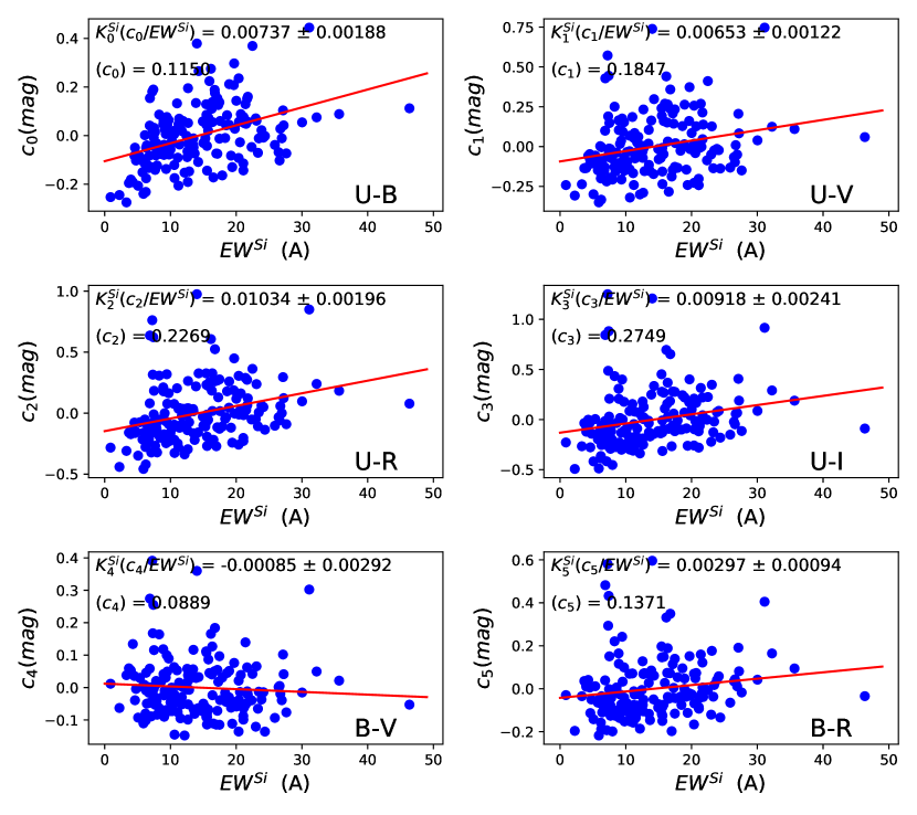
Figure 1: Correlations between the first five colours $c_{0}^{\prime}\equiv U-B$, $c_{1}^{\prime}\equiv U-V$, $c^{\prime}_{2}\equiv U-R$, $c^{\prime}_{3}\equiv U-I$, $c^{\prime}_{4}\equiv B-V$, $c^{\prime}_{5}\equiv B-R$ (mag) and $\textup{ew}^{\textup{Si}}$ (Å). The slopes of the straight line fits (red lines) give the value of $K^{\textup{Si}}$ directly. The correlations of the colours can be derived from the first four.

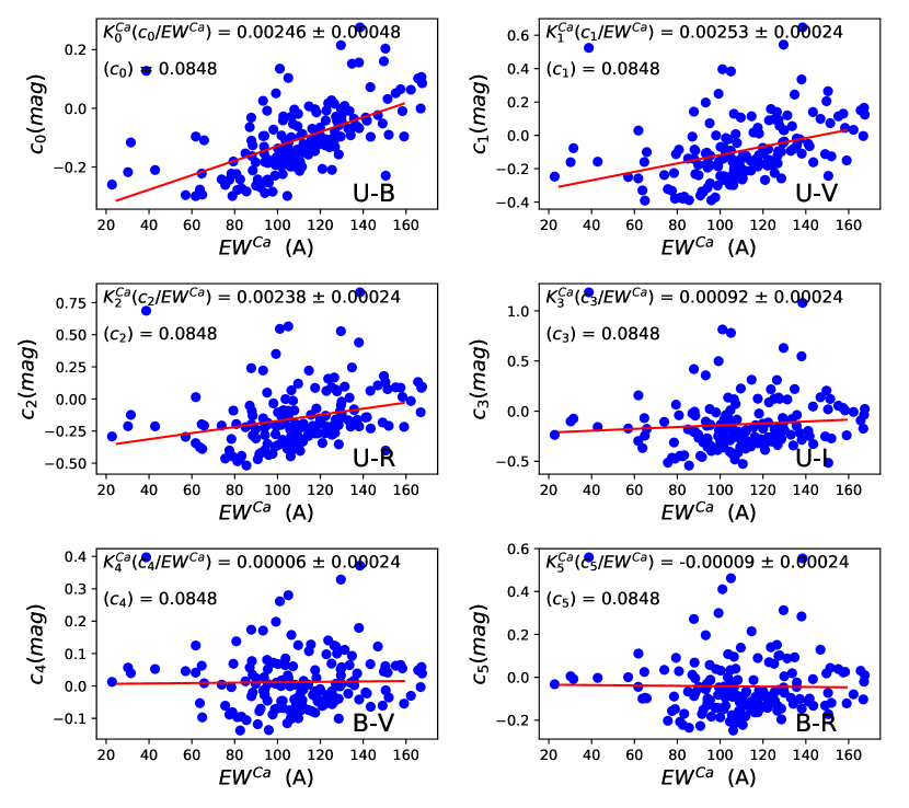
Figure 2: Correlations between the same colours as Fig. 1, corrected for the $\textup{ew}^{\textup{Si}}$ correlation (mag), as a function of $\textup{ew}^{\textup{Ca}}$ (Å). The slopes of the straight line fits (red lines) give the value of $K^{\prime\textup{Ca}}$.

Table 3: Colour correction from $\textup{ew}^{\textup{Si}}$ and $\textup{ew}^{\textup{Ca}}$. The first four colours allow the prediction of the coefficients $K^{\textup{Si}}$ and $K^{\textup{Ca}}$ for the other ones. The coefficients $\sigma$ and $\kappa$ are then derived via Eq. 10.

	colour	$K^{\textup{Si}}$	$K^{\prime\textup{Ca}}$	$\sigma_{i}$	$\kappa_{i}$
		(mag/Å)	(mag/Å)	(mag/Å)	(mag/Å)
0	$U-B$	$0.00737\pm 0.00122$	$0.00246\pm 0.00027$	$0.00608\pm 0.00123$	$0.00251\pm 0.000295$
1	$U-V$	$0.00653\pm 0.00195$	$0.00253\pm 0.00049$	$0.00520\pm 0.00196$	$0.00258\pm 0.000501$
2	$U-R$	$0.01034\pm 0.00241$	$0.00238\pm 0.00063$	$0.00910\pm 0.00243$	$0.00242\pm 0.000687$
3	$U-I$	$0.00918\pm 0.00292$	$0.00092\pm 0.00079$	$0.00870\pm 0.00295$	$0.00934\pm 0.000806$

As shown in Sect. 9, we found that the correction of colours for spectral features was necessary. The parameters $\sigma_{i}$ and $\kappa_{i}$ could be considered as additional parameters of the model implemented, though they are not tuned but measured; we show in Sect. 9 that the Ca-Si colour correction is closely related to the SALT variable $x_{1}$.

4.2 Evaluation of extinction coefficients $\delta$

4.2.1 From extinction formula to coefficients $\delta$

This section describes the contribution of the reddening to the colour variations. Our reddening indicator is the extinction part $X_{4}$ (defined in Eqs. 3, 4) of $e_{4}=E(B-V)-\langle E(B-V)\rangle$ after the $\textup{ew}^{\textup{Ca}}$ and $\textup{ew}^{\textup{Si}}$ corrections have been applied; its mean $\langle X_{i}\rangle$ is zero, and it can have a positive or negative sign, but its variations are the same as the standard one (up to the intrinsic contributions of $\textup{ew}^{\textup{Si}}$, $\textup{ew}^{\textup{Ca}}$, and $I_{i}$, which we do want to exclude from the extinction correction). The SNfactory top-hat filters are defined in Table 1, and the extinction formula is (at first) assumed to be perfectly known, as given by FM99, once a value of $R_{V}$ is chosen, which we assume until Sect. 7.

The reddening corrections $A^{\prime}_{F}$ and $R^{\prime}_{Fi}$ of Eq. 4.2.1 for the bandpass $F$ are then evaluated for each value of $R_{V}$ in a grid, and the analysis described in this section is repeated over the grid. The difficulty that we address is that the extinction indicator $E_{n}(B-V)$ (with or without subtraction of the mean) is always tied to the choice of a wide bandpass, top-hat (our case), or Bessell. The reddening corrections at each wavelength depend on wavelength and $R_{V}$, but also on the choice of wide band filter, and on the spectral shapes of the selected stars through the wide-band integration. The rest-frame photon-count spectrum $s_{n}(\lambda)$ for SN $n$ is

$$s_{n}(\lambda)=s_{0}(\lambda)\,10^{-0.4\phi(\lambda)\,E_{n}(B-V)}.$$ (11)

With the colour difference definition $E_{n}(B-V)=(B-V)_{n}-\langle B-V\rangle$, the spectrum $s_{0}(\lambda)$ at null colour difference is the mean SN Ia photon-count spectrum; the function $\phi(\lambda)$ is provided by Cardelli et al. (1989); O’Donnell (1994); Fitzpatrick & Massa (2005). This extinction indicator $E_{n}(B-V)$, or ‘colour difference’, differs by a constant term from the standard $E(B-V),$ which is referenced to the zero extinction value rather than the mean; the extinction indicator $E_{n}(B-V)$ can be positive or negative. This constant shift (bandpass-dependent) affects colours, but not their variations, with which we deal exclusively. Equation 11 is a slight extension of the standard extinction formula of FM99 on two counts: the extinction formula relies on a specific set of blue stars, not SNe, and the bandpasses are defined by Bessell filters, rather than top-hat filters as described in Table 1. This issue is addressed in Sect. 4.2.2. Hereafter, we use the extinction component of $E_{n}(B-V)$, that is, $X_{4}(n)=X_{B-V}(n)$, as a substitute for the colour difference $E_{n}$ in Eq. 11. It is shown in Appendix A that, in the linear approximation, the extinction correction $A^{\prime}_{F}$ in filter $F$ is given for a SN with photon-count spectrum $s(\lambda)$ by:

$$A^{\prime}_{F}(n) =m_{F}^{\text{obs}}(n)-m_{F}^{\text{true}}(n)$$

$$\simeq R^{\prime}_{F4}X_{4}(n)=\frac{\int_{F}s_{0}(\lambda)\phi(\lambda)\,\textup{d}\lambda}{\int_{F}s_{0}(\lambda)\,\textup{d}\lambda}X_{B-V}(n).$$ (12)

The coefficient $R^{\prime}_{F4}$ is the exact derivative of the reddening correction $A^{\prime}_{F}(n)$ with respect to the extinction colour component $X_{4}$ at $X_{4}=0$. We show in Table 12 that the relative error resulting from this approximation remains smaller than 0.01 over the full range of values of $X_{4}$. The reddening correction coefficient $A^{\prime}_{F4}$ should actually be weighted by the spectrum of each SN according to Eq. 4.2.1, but as we only consider a linear reddening correction, the SN dependence would bring a negligible second-order correction. The term $X_{B-V}(n)=X_{4}(n)$ in Eq. 4.2.1 is the extinction content of the colour difference $e_{4}=E_{n}(B-V)$ for SN $n$. As noted previously, the extinction colour $X_{i}(n)$ can be positive or negative, but should be a better reddening indicator than $E_{n}(B-V)$ as the intrinsic colour variation has been removed.

For each bandpass $F=UBVRI$, the extinction coefficient $R^{\prime}_{F4}=A^{\prime}_{F}/X_{B-V}(n)$ is obtained from Eq. 4.2.1. The associated colour differences are $e_{i}={c_{i}}-\langle c_{i}\rangle$. The extinction coefficients $R^{\prime}_{Fj}$ ($j\neq 4$) are then derived from the integrated extinction formula. The value of $R^{\prime}_{Fi}$ for another colour $i$ can be derived from $R^{\prime}_{F4}$; for example $R^{\prime}_{F3}$ (with $e_{3}\equiv U-I$) is given by:

$$R^{\prime}_{F3}=\frac{R^{\prime}_{F4}}{R^{\prime}_{U4}-R^{\prime}_{I4}}.$$ (13)

The colour–colour coefficients $\delta^{\prime}_{ij}$ relate the (extinction) colour excesses of all colours; they are obtained from the two bandpasses defining each colour, from the analogue of Eq. 13; for example, for $e_{2}\equiv U-R$ and $e_{6}\equiv B-I$, one has $X_{2}=\delta_{24}X_{4}=\delta_{26}X_{6}$ with

$$\delta_{26}=R^{\prime}_{U6}-R^{\prime}_{R6}=\frac{R^{\prime}_{U4}-R^{\prime}_{R4}}{R^{\prime}_{B4}-R^{\prime}_{I4}}.$$ (14)

The extinction correction for all the other colours is similar. The colour indicators used in this study is actually the extinction component $X_{B-V}$ of $B-V$ computed in Sect. 5.2 rather than the measured value $e_{B-V}$. For instance, the correction to $e_{5}\equiv B-R$ using $X_{6}\equiv B-I$ is

$$X_{5}=\delta_{56}(R_{V})\,X_{6}=\frac{R^{\prime}_{B4}-R^{\prime}_{R4}}{R^{\prime}_{B4}-R^{\prime}_{I4}}X_{6}=\delta_{54}(R_{V})\,X_{4}.$$ (15)

Using for instance the extinction part $X_{4}$ of colour $4\equiv B-V$ or the extinction part $X_{6}$ of colour $6\equiv B-I$:

$$m_{F}(n)^{\text{corr}} =m_{F}(n)^{\text{obs}}-A^{\prime}_{F}(n)(R_{V})$$ (16)

$$A^{\prime}_{F}(n,R_{V}) =\delta^{\prime}_{F4}(R_{V})\,X_{4}(n)=\delta^{\prime}_{F6}(R_{V})\,X_{6}(n).$$ (17)

(We recall that $m_{F}^{\text{obs}}(n)$ has been brought to a common reference redshift.)

4.2.2 Rescaling of extinction coefficients: from $\delta^{\prime}$ to $\delta$

The extinction formulae, such as those of Cardelli et al. (1989) or FM99, have not been tuned for SN spectra, nor to our set of top-hat bandpasses. In addition, the extinction law was established for a sample of mostly HD stars, where the extinction of each spectral bin is weighed by a spectrum that differs from the SNe Ia spectrum. It should not be assumed that the extinction formulae provided by Cardelli et al. (1989); O’Donnell (1994); Fitzpatrick & Massa (2005) —with different filters (Bessell) and different stars (HD)— apply directly to SNe Ia, given the presence of the wide band term $E_{n}(B-V)$ or $X_{4}(n)$ in Eq. 11. The minimal correction proposed here is a rescaling of the formula so as to ensure consistency. If we apply Eq. 4.2.1 to $e_{4}=E_{n}(B-V),$ we find $e_{4}=(R^{\prime}_{B4}-R^{\prime}_{V4})e_{4}$ (or $X_{4}=[R^{\prime}_{B4}-R^{\prime}_{V4}]X_{4}$). We must expect

$$R^{\prime}_{B4}-R^{\prime}_{V4}=1.$$ (18)

If the extinction in the $V$ bandpass is used —which is a frequent occurrence— a different consistency condition should be implemented: $R^{\prime}_{V4}=1$ to ensure that $A_{V}$ is the actual extinction in this bandpass. Equation 18 is sometimes written (e.g. Mandel et al. 2017; Jha et al. 2007) as $R_{B}-R_{V}=1$. However, we find (for $R_{V}=2.25$) with the previously defined top-hat bandpasses $(R^{\prime}_{B4}-R^{\prime}_{V4})_{FM99}=0.864$, while with O’Donnell (1994) extinction parameters, $(R^{\prime}_{B4}-R^{\prime}_{V4})=0.814$. Most of this difference is due to the Bessell bandpasses assumed in the extinction formula, while we are using top-hat filters in the present study. Indeed, when using Bessell filter weighting (Bessell & Murphy 2012), $R^{\prime}_{B4}-R^{\prime}_{V4}=1.0329$, which is closer to but still incompatible with unity. We show in Eq. 45 of the Appendix that the expression of the coefficient $R^{\prime}_{F4}$ in Eq. 4.2.1 is the exact derivative of the reddening correction with respect to the extinction colour at $X_{4}=X_{B-V}=0$, and in Table 12 that the linear approximation is accurate to within $5\,10^{-3}$ mag over the full range of extinctions. Another contribution to this mismatch may be the different spectra of stars used in FM99 and in the present work (SNe Ia). We assume that an acceptable correction ensuring the ‘consistency condition’ in Eq. 18 is an overall rescaling of the extinction formula at all wavelengths, so as to force $R_{B4}-R_{V4}=1$. All the coefficients $R^{\prime}_{Fi}$ are rescaled:

$$R_{Fi}=R^{\prime}_{Fi}/(R^{\prime}_{B4}-R^{\prime}_{V4}).$$ (19)

The extinction coefficient of each filter is then increased by the factor $1/(R^{\prime}_{B4}-R^{\prime}_{V4})=1/0.864$. No such global rescaling was applied in C11 where an extinction parameter $A_{V}$ was fit independently for each SN. As mentioned above, Eq. 11 is only an approximation. Even if one accepts that different molecular and grain compositions can be summarised by a single coefficient $R_{V}$ (related to their cross section for light), its value could differ in the halo and in the disc (if there is one), and the observations of Schlafly et al. (2016) in our own galaxy suggest this possibility. The $\delta_{ij}$ coefficients of Eq. 4 verify that $\delta_{ij}=1/\delta_{ji}$. The five values of the extinction coefficients $\delta_{F4}(R_{V}),$ which provide the extinction in filters for $F=UBVRI$ from $X_{4}=X_{B-V}$, are given in Table 4. The extinction coefficients $\delta_{F}(R_{V})$ are subject to a first correction ($\operatorname{Dex}_{F}$), which cancels the correlations of the colour residuals with the extinction components as discussed in Sect. 5.4; they are then rescaled for algebraic consistency as described in Eq. 19. Finally, for arbitrary values of $R_{V}$, the suppression of the correlation of extinction-corrected magnitudes with the extinction colour in the $V$ bandpass requires an extra overall rescaling $s,$ which is a function of the extinction parameter $R_{V}$, as explained in Sect. 7. Such a scaling destroys the consistency condition in Eq. 18, but is introduced in practice by almost all authors (Boone et al. 2021; Chotard et al. 2011; Amanullah et al. 2015; Saunders et al. 2018; Thorp et al. 2021) who substitute $m_{F}^{\text{corr}}(\lambda)=m_{F}^{\text{obs}}(\lambda)-A_{V}\,\phi(\lambda,R_{V})$ where $A_{V}$ is arbitrary and $\phi(\lambda,R_{V})$ stands for one of the reddening formula. The analysis of the extinction is performed over a grid of nine values of $R_{V}$: $1.95,2.05,2.15,2.20,2.25,2.35,2.50,2.60$, and $3.10$. We show below that for our value of $R_{V}$, the scaling factor $s$ is indeed compatible with unity, which confirms the consistency of the model, as well as the value of $R_{V}$ obtained.

Table 4: Extinction coefficients from FM99 and $UBVRI$ corrections to the extinction formula for the case $R_{V}=2.25$. In the second line, the extinction formula values are modified as explained in Sect. 5.4.

$R_{F4}$	$U$	$B$	$V$	$R$	$I$
FM99 $R^{\prime}_{F4}$	3.9232	3.2477	2.3832	1.6914	1.2167
Modified (Sec. 5.4) $R_{F4}$	3.9907	3.2062	2.3397	1.7910	1.1161
Scaled (Eq. 19)	4.6057	3.7003	2.7003	2.0671	1.2881

5 Extraction of intrinsic and extinction colour components

5.1 Intrinsic colour coefficients $\gamma$

As mentioned in Eq. 3, the colour difference $e_{i}(n)$ of SN $n$ (after correction for $\textup{ew}^{\textup{Si}}$ and $\textup{ew}^{\textup{Ca}}$) is the sum of two components $e_{i}(n)=I_{i}(n)+X_{i}(n)+\epsilon_{i}(n)$, and the intrinsic component $I_{i}$ of colour $i$ is assumed to belong to a one-dimensional space of intrinsic colour fluctuations, as suggested by Léget et al. (2020) and Boone et al. (2021). These are then interrelated by a set of coefficients $\gamma_{ij}$ common to all supernovæ $n$ as introduced in Eq. 4. As shown below, small corrections to the extinction formula are required. An initial value for the coefficients $\gamma_{ij}$ can be derived directly from the requirement that intrinsic and extrinsic colours be uncorrelated, though this value can differ significantly from the result of the $\chi^{2}$ minimisation discussed later. For any pair of leading ($i$) and auxiliary ($j$) colour, two equations link $X_{i},X_{j}$ and $I_{i},I_{j}$:

$$e_{i} =I_{i}+X_{i}+\epsilon_{i}=\gamma_{ij}I_{j}+\delta_{ij}X_{j}+\epsilon_{ij},$$ (20)

$$e_{j} =I_{j}+X_{j}+\epsilon_{j}.$$ (21)

The initial values of $\gamma_{i0}$ can be obtained from the previous equations, assuming the absence of correlations between the $I_{i}$ and the $X_{i}$, and neglecting the contribution of the residuals $\epsilon_{i}$ and $\epsilon_{ij}$,

$$\langle e_{1}^{2}\rangle =\gamma_{10}^{2}\langle I_{0}^{2}\rangle+\delta_{10}^{2}\langle X_{0}^{2}\rangle,$$ (22)

$$\langle e_{0}^{2}\rangle =\langle I_{0}^{2}\rangle+\langle X_{0}^{2}\rangle,$$ (23)

$$\langle e_{0}\,e_{1}\rangle =\gamma_{10}\langle I_{0}^{2}\rangle+\delta_{10}\langle X_{0}^{2}\rangle.$$ (24)

Here, $\delta_{ij}$ is the ratio of the extinction components $X_{i}/X_{j}$, as defined in Table 2 —and is not the Kronecker $\delta$—, and the index $n$ of the SN is dropped.

Combining Eq. 23 ($\times\delta_{10}$) and 24, one gets $\langle e_{0}\,e_{1}\rangle-\delta_{10}\langle e_{0}^{2}\rangle=(\gamma_{10}-\delta_{10})\langle I_{0}^{2}\rangle$. Similarly, $\langle e_{1}\rangle^{2}-\delta_{10}\langle e_{0}\,e_{1}\rangle=\gamma_{10}(\gamma_{10}-\delta_{10})\langle I_{0}^{2}\rangle$; dividing the two previous relations one obtains an initial value of $\gamma_{10}$ (with large errors). More generally, an initial value for any pair of colours would be:

$$\gamma_{ij}=\frac{\langle e_{i}^{2}\rangle-\delta_{ij}\langle e_{i}\,e_{j}\rangle}{\langle e_{i}\,e_{j}\rangle-\delta_{ij}\langle e_{j}^{2}\rangle}.$$ (25)

The initial values of the three coefficients $\gamma_{10}$, $\gamma_{20}$, and $\gamma_{30}$ are respectively 0.671, 0.759, and 0.401. The statistical errors on these initial values are relatively large, and an improved determination is obtained from the iterative fits described in the following section. (We recall that all colour differences have zero average, and that intrinsic and extinction components are assumed to be uncorrelated.)

Given the relation $\delta_{ij}=1/\delta_{ji}$, we find that (as expected) $\gamma_{ij}=1/\gamma_{ji}$. The coefficients $\gamma_{ij}$ can be expressed according to Eq. 4 in terms of three of them, which have been selected as $\gamma_{10}=I_{(U-V)}/I_{(U-B)}$, $\gamma_{20}=I_{(U-R)}/I_{(U-I)}$, and $\gamma_{30}=I_{(U-I)}/I_{(U-B)}$. The remaining 42 coefficients can be obtained from the following relations, which result from the algebraic relations between colours:

$$\gamma_{40} =-1+\gamma_{10}, \gamma_{50} =-1+\gamma_{20}, \gamma_{60} =-1+\gamma_{30},$$

$$\gamma_{70} =-\gamma_{10}+\gamma_{20}, \gamma_{80} =-\gamma_{10}+\gamma_{30}, \gamma_{90} =-\gamma_{20}+\gamma_{30},$$ (26)

$$\gamma_{ik} =\gamma_{i0}/\gamma_{k0}.$$

5.2 $\chi^{2}$ for intrinsic and extinction colour components

The model described by Eq. 20 should reproduce the rest-frame colours. We consider the colour difference for SN $n$: $e_{i}(n)=c_{i}(n)-\langle c_{i}\rangle$. The two components $(I_{i}(n),X_{i}(n))$ can be found by requiring that all colours $e_{j}(n)$ are properly described by Eqs. 20–21, and the coordinates $I_{j}(n)=\gamma_{ji}I_{i}(n)$, $X_{j}(n)=\delta_{ji}X_{i}(n)$. Colour components $X_{2}(n)$ and $I_{2}(n)$ are, for example, obtained by minimising —for each SN $n$— the $\chi^{2}_{2}(n)$ in Eq. 29 as a function of the ‘coordinates’ $I_{2}(n)$ and $X_{2}(n)$. The reddening correction $A_{V}(n)$ in bandpass $V$ $A_{V}(n)=R_{V4}X_{4}(n)$, which varies from SN to SN, plays no role in the minimisation: the extinction correction is $A_{F4}(n)=R_{F4}X_{4}(n)$ for filter $F$ and SN $n$ ($=A_{Fi}(n)=R_{Fi}X_{i}(n)$ using another colour):

$$\epsilon_{2} =X_{2}+I_{2}-e_{2},$$ (27)

$$\epsilon_{k2} =(\gamma_{k2}I_{2}+\delta_{k2}X_{2}-e_{k}),$$ (28)

$$\chi^{2}_{2} =\epsilon_{2}^{2}+\sum_{k\in Aux}\epsilon_{k2}^{2},$$ (29)

as a function of $I_{2}$ and $X_{2}$, under the constraint

$$\sum_{\text{all SNe}}I_{2}(n)\,X_{2}(n)=0.$$ (30)

Equation 30 imposes the decorrelation of the extra-intrinsic colour from extinction. The index $n$ is omitted in Eq. 27. For each colour $i$ and each SN, the residual $\epsilon_{i}(n)$ defined by Eq. 27 should not be confused with the magnitude shift at maximum light defined in Eq. 2. We are aware that Eq. 30 could be criticised under certain circumstances, such as in the presence of circumstellar matter with a composition differing from the average host galaxy. Such matter, as pointed out by Borkowski et al. (2009); Ferretti et al. (2017), might invalidate this assumption, but if the circumstellar dust is created by a non-degenerate companion, as suggested in one case by Nagao et al. (2017), it is not necessarily correlated to the SN Ia properties. While not rejecting the possibility, we wanted to explore the accuracy that could be reached within the assumption of decorrelation.

Each pair $(I_{i}(n),X_{i}(n))$ of components allows the prediction of all the other colours of the SN. When defining $\chi^{2}(n)$ in Eq. 29, each colour $i$ enters with equal weight, which implicitly assumes that the errors on all colours are similar. The solution of Eq. 29 in terms of $(X_{2}(n),Y_{2}(n))$ is found by requiring $\partial\chi_{2}^{2}/\partial X_{2}=\partial\chi_{2}^{2}/\partial I_{2}=0$:

$$\left(\begin{array}[]{c}Y_{0}\\ Y_{1}\end{array}\right)=\left(\begin{array}[]{c c}M_{00}&M_{01}\\ M_{10}&M_{11}\end{array}\right)\left(\begin{array}[]{c}I_{2}\\ X_{2}\end{array}\right)$$ (31)

with

$$M_{00} =1+\sum_{k\in Aux}\gamma_{k2}^{2}, M_{01} =1+\sum_{k\in Aux}\gamma_{k2}\delta_{k2}-\lambda,$$

$$M_{10} =M_{01}, M_{11} =1+\sum_{k\in Aux}\delta_{k2}^{2},$$ (32)

$$Y_{0} =e_{2}(k)+\sum_{k\in Aux}\gamma_{k2}\,e_{k}, Y_{1} =e_{2}(k)+\sum_{k\in Aux}\delta_{k2}\,e_{k}.$$

The colours excesses $e_{1}(n)$ and $e_{2}(n)$ are measured, meaning that $Y_{0}$ and $Y_{1}$ are known. The intrinsic and extinction components $I_{2}(n)$, $X_{2}(n)$ are obtained by inverting Eq. 31. The Lagrange multiplier $\lambda$ arises from the assumption of uncorrelated $I_{i}$, $X_{i}$, and is found from Eq. 30; it depends on the colour, but is the same for all SNe. We introduce the set $Aux$ of auxiliary colours used to extract the intrinsic and extinction components of each colour. In the optimisation of the intrinsic couplings $\gamma_{ij}$ below, the full set of ten colours cannot be used in view of the appearance of algebraic constraints, as explained in the following section. Table 5 presents the actual list of auxiliary colours used for each colour. There is an arbitrariness in the choice of the participating colours in $Aux$; we selected the one that yielded the smallest residuals among five trials.

For each SN $n,$ this minimisation yields ten intrinsic colours $I_{i}(n)$, and ten extinction colours $X_{i}(n)$, once the intrinsic colour coefficients $(\gamma_{01},\gamma_{02},\gamma_{03})$ are known. Equation 29 does not take into account the correlation between colours, but as the solution gave acceptable residuals for all colours, we kept this simplified expression for $\chi^{2}$. We verified that including the obvious algebraic correlations between the different colours does not change the solution, but it does add significant complications. As the mean of $e_{i}$ is zero (by definition), the mean values of $I_{i}$ and $X_{i}$ obtained by linear combinations of $e_{i}$ will also be zero.

Table 5: Map of the auxiliary colours used in Eq. 29 and Eq. 32. The first column is the measured colour being adjusted by the model. Colours 5 and 7, which have a small intrinsic part, are not included in the evaluation of other colours. The sample of auxiliary colours with the smallest mean residual was selected.

Colour index	Auxiliary colours
0	1, 2, 3, 4, 6, 9
1	0, 2, 3, 4, 6, 8
2	0, 1, 3, 4, 6
3	0, 1, 2, 4, 6, 8, 9
4	0, 1, 2, 3, 4, 6
5	0, 1, 2, 6, 8, 9
6	0, 2, 3, 4, 8, 9
7	1, 2, 3, 4, 6, 8, 9
8	1, 3, 4, 6, 9
9	2, 3, 4, 6, 8

5.3 Determination of intrinsic components and intrinsic couplings

The colour differences which we now use were subtracted from the contributions of Ca and Si, but leave room for an extra-intrinsic component $I_{i}$ of each colour, with all of them dependent on three parameters ($\gamma_{10}$, $\gamma_{20}$, $\gamma_{30}$) as required by the assumption of a single extra-intrinsic contribution. Up to this stage, the $\gamma_{ij}$ are obtained from their initial values in Eq. 25. The solution of Eq. 31 is only acceptable if the ratio of the solutions of Eq. 31 $I_{i}(n)$ to $I_{j}(n)$ for two colours $i$ and $j$ is equal to $\gamma_{ij}$ for all SNe and all pairs of colours. Similarly, the ratio of $X_{i}(n)$ to $X_{j}(n)$ should be equal to $\delta_{ij}$.

This is achieved by a sequence of iterations. At each iteration, and for each colour, the input coefficients $\gamma_{ij}^{\text{in}}$ are the parameters introduced in Eqs. 4 and 28, while the linear coefficients of the straight line fits in the plane $(I_{i},I_{j})$ as in Fig. 3 are the output value $\gamma_{ij}^{\text{out}}$ of the intrinsic couplings. The output values of ($\gamma_{10},\gamma_{20},\gamma_{30}$) are reinjected into Eq. 29 until Fig. 3 is satisfactory. The scatter is seen to range from 0.002 mag to 0.01 mag depending on the colours, and the measured values of the ratios $\gamma_{ij}^{\text{out}}=I_{i}/I_{j}$ are within 0.01 of the corresponding set of $\gamma_{ij}^{\text{in}}$, as obtained from $(\gamma_{10},\gamma_{20},\gamma_{30})$ using Eq. 5.1. The $\delta_{ij}$ coefficients are left unchanged in this sequence, as their values are fixed by the extinction formula (at this stage).

We then turn to Fig. 4, which compares the full set of input values $\gamma_{ij}^{\text{in}}$ in Eq. 31 in the second-to-last iteration to the output values, that is, of $I_{i}/I_{j}$ from the linear fits in Fig. 3. The final values of the three coefficients ($\gamma_{10}^{\text{out}}$, $\gamma_{20}^{\text{out}}$, $\gamma_{30}^{\text{out}}$) are found by minimising the scatter (RMS) of the output coefficients $\sigma(\gamma_{ij}^{\text{out}})$ with respect to the input coefficients (horizontal scale). This last step brings in the constraint of consistency with Eq. 5.1 for the whole set of $\gamma_{ij}$, and modifies the result of the previous sequence of iterations; however, as seen in Fig. 3, the outcome is still satisfactory with respect to the convergence of the solution for each $\gamma_{ij}$

The relation between $\gamma_{ij}^{\text{out}}$ and $\gamma^{\text{in}}_{ij}$ is shown in Fig. 4 at the last iteration. The linear coefficient is expected to be close to unity if convergence has been achieved, while we find 1.00069, with an RMS of 0.0104. This dispersion arises from a combination of measurement errors, Si-Ca correction errors, and modelling errors. Two precautions were implemented to extract the three intrinsic couplings from Eq. 31 and Fig. 4: we eliminated the auxiliary colours $4\equiv B-V$ and $7\equiv V-R$ that have very small intrinsic components (cf. Table 9) from the $10\times 9/2=45$ $\gamma_{ij}$ couplings, 28 remain after the elimination of colours 5 and 7. The 28 output values of the parameters $\gamma^{\text{out}}_{ij}=I_{i}/I_{j}$ at the last iteration are compared in Fig. 4 to the input values derived from ($\gamma_{10}$, $\gamma_{20}$, $\gamma_{30}$) using Eq. 5.1. The equality of input and output values was not forced into the optimisation process. The ratios $\delta_{ij}=X_{i}/X_{j}$ are also seen to have a small scatter of 0.002 mag (in Fig. 3), with averaged output values close to the input coefficients, supporting the model Eqs. 27–29.

Nevertheless, the RMS in Fig. 4 fails as an indicator when the same set of colours (auxiliary and main) is used to find the intrinsic content, as the algorithm defined by Eq. 31 yields $\sigma(\gamma^{\text{out}}_{ij})=0$. For each colour, we eliminated at least one extra auxiliary colour to avoid such duplicated sets. The choice of the auxiliary colours has an impact on the values found for the three intrinsic couplings. We selected the one that gave the smallest mean residual scatter (RMS) in Fig. 4. The scatter of $\gamma_{ij}^{\text{out}}$ in Fig. 4 is 0.0103, and the ratio $\gamma^{\text{out}}_{ij}/\gamma^{\text{in}}_{ij}$ is within 0.001 of unity. After the sequence of iterations described in Sect. 5.4, the optimal values in Fig. 4 for $R_{V}=2.20$ are given in Table 6.

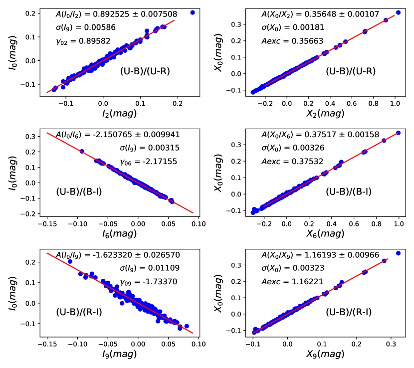
Figure 3: Intrinsic $\gamma^{\text{out}}_{0i}=I_{0}/I_{i}$ and extinction $\delta^{\text{out}}_{0i}=X_{0}/X_{i}$ ratios as defined in Eq. 31 $(i=2,6,9)$ compared to the input $\gamma^{in}_{0i}$ and calculated $\delta_{0i}$ for $R_{V}=2.25$. The compatibility is at the level of 0.001 for the extinction, and the relative accuracy of 0.05 for the (smaller) intrinsic colour (worst case). The red lines are linear fits to the data, and $\gamma^{\text{out}},\delta^{\text{out}}$ are the values of the linear coefficients.

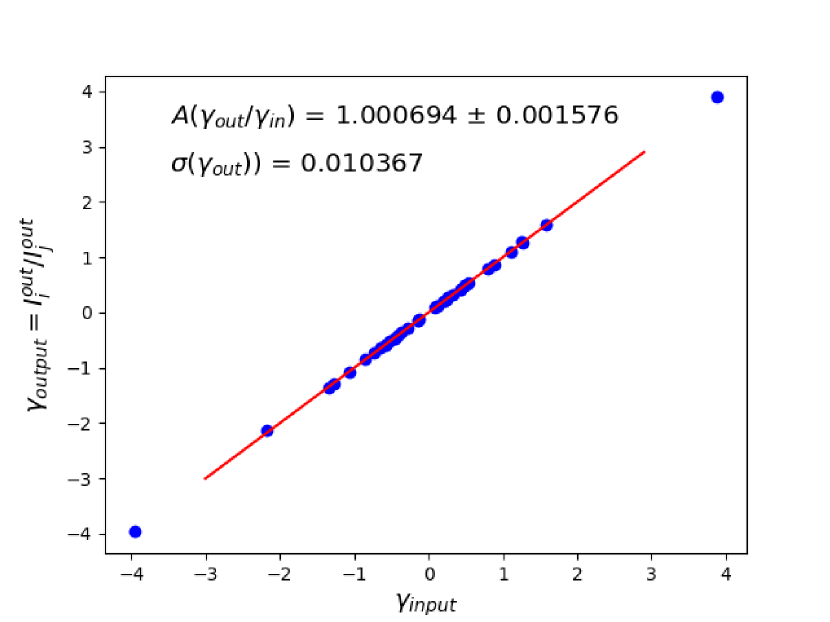
Figure 4: Relation between input and output ($\langle I_{i}/I_{j}\rangle$) values for the coefficients $\gamma_{ij}$. The overall agreement for all $\gamma_{ij}$ (excluding those involving colours $5\equiv(B-R)$ and $7\equiv(V-R)$) is within 0.01.

Table 6: Coupling constants of the intrinsic colours.

$R_{V}$	$\gamma_{10}$	$\gamma_{20}$	$\gamma_{30}$
$2.20$	$1.2687\pm 0.0586$	$1.1248\pm 0.0134$	$0.5579\pm 0.0286$
$2.25$	$1.2647\pm 0.0586$	$1.1163\pm 0.0134$	$0.5395\pm 0.0286$

The errors are derived at this stage from the spread of the results in four different choices of auxiliary colours and do not include the statistical error. The comparison of our intrinsic colours to previous results is postponed to Sect. 9, as the contribution of the equivalent widths $\textup{ew}^{\textup{Ca}}$ and $\textup{ew}^{\textup{Si}}$ must be reintroduced.

5.4 Modifications to the extinction formula

For all values of $R_{V}$, the colour residuals $\epsilon_{i}$ described in the previous section (after Eq. 29) show a strong correlation with the extinction colour component when the FM99 extinction formula is used. This (unexpected) correlation is apparent in Fig. 5, and there is no value of $R_{V}$ that suppresses this effect. As our subsequent determination of $R_{V}$ relies on the absence of any correlation between the extinction-corrected magnitudes and the extinction, it is crucial to suppress the correlation observed in Fig. 5. This suppression depends on the coefficients $\gamma_{ij}$ and $\delta_{ij}$ in Eq. 32 but in no way on the scale of the reddening correction (nor on the rescaling applied in Eq. 19).

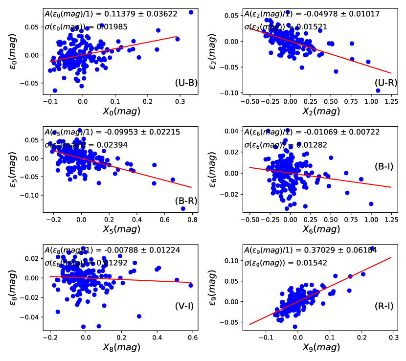
Figure 5: Correlation of the colour residuals (mag) for $R_{V}=2.25$ with the extinction colour for colour differences $e_{0},e_{2},e_{5},e_{6},e_{8},e_{9}$ (no extinction formula correction). The strong correlations observed would forbid a safe evaluation of $R_{V}$.

We can cancel the effects observed in Fig. 5 by introducing corrections $\operatorname{Dex}_{F}$ to the extinction coefficients $R_{F4}$ of the five $F=UBVRI$ bandpasses in Eq. 4.2.1. The minimised quantity is

$$\chi_{\operatorname{Dex}}^{2}=\sum_{i=0}^{9}(sl_{i})^{2}\qquad\text{with}\qquad sl_{i}=\partial\epsilon_{i}/\partial X_{i}.$$ (33)

The extinction corrections $\operatorname{Dex}_{F}$ in the five filters are applied to the values of $R^{\prime}_{F4}$ from Eq. 4.2.1: $R^{\prime}_{F4}\to R^{\prime}_{F4}+\operatorname{Dex}_{F}$ and fitted for each value of $R_{V}$ so as to minimise $\chi_{\operatorname{Dex}}^{2}$, and cancel the coefficients $sl_{i}$ in Fig. 5. The result is given in Table 7. As there is an overall scale degeneracy of the extinctions in the colour analysis, we arbitrarily set the $U$ bandpass correction to be 0.0675. At each value $R_{V}$ of the grid, the corrections are evaluated. As these corrections (partially) compensate for the distortions introduced by the difference between the ‘optimal $R_{V}$’ and the value used in the grid, they tend to blow up when $R_{V}$ is close to the limits of the range considered in this work, namely as $R_{V}\to 1.95$ or $R_{V}\to 3.10$. The offsets are applied in the second line of Table 4. The impact of these corrections on the correlation between the residuals and the extinction is shown in Fig. 6, and for all colours in Table 8. The large value of $sl_{9}$ observed ($e_{9}\equiv R-I$) in Fig. 5 reflects the significant corrections to the extinction formula in bandpasses $R$ and $I$, with opposite signs. The errors given in these figures are only indicative, as somewhat arbitrary ‘floor’ errors of 0.006 mag are imposed on the determination of the extinction colour.

Table 7: $UBVRI$ corrections (mag) to the extinction formula. The number of decimals describes the convergence criterion, not the (lower) accuracy of the results. The choice of the $U$ correction is arbitrary.

$R_{V}$	$\operatorname{Dex}_{U}$	$\operatorname{Dex}_{B}$	$\operatorname{Dex}_{V}$	$\operatorname{Dex}_{R}$	$\operatorname{Dex}_{I}$	$\gamma_{10}$	$\gamma_{20}$	$\gamma_{30}$
	(mag)	(mag)	(mag)	(mag)	(mag)
2.20	0.0675	$-0.03679$	$-0.03923$	0.1013	$-0.11126$	1.2687	1.1248	0.5579
2.25	0.0675	$-0.04147$	$-0.04351$	0.1015	$-0.11090$	1.2647	1.1163	0.5395

The corrections to the extinction formula are extremely unlikely to be caused by the limitations of our model: The linear approximation involved is numerically correct to better than 0.005 mag in the whole range of $e_{4}=E(B-V)$ considered. There could be a second intrinsic colour involved; that is, rather than one-dimensional (beyond Ca and Si), as in Eq. 4, the intrinsic colour space could be two-dimensional, with a second set of $\gamma_{ij}$ coefficients, but intrinsic colours are uncorrelated (or are at best weakly correlated) to extinction, and this new intrinsic colour would have to be larger than the one already introduced to make up for the 0.10 mag discrepancies observed in Fig. 5. There is no room in the residuals for such a large extra-intrinsic component. On the other hand, the need for an adaptation of the extinction formula to SNe and Top-hat filters is shown in Sect. 4.2.2, where the presence of a rescaling factor is first introduced.

The numerical value of the corrections are dependent on the specific bandpasses involved, on the spectral template, and also possibly on the dust properties of our galaxy, which may differ from the averaged dust extinction. Figure 6 shows that, after correction, the remaining correlations of the residuals $\epsilon_{i}$ with extinction are negligible. This can be achieved regardless of the value of $R_{V}$. The largest of these effects amounts to a residual linear dependence of 0.006 for $B-V$. The coefficients of all other colours are smaller than 0.0036. The statistical errors on the offsets away from the extinction formula for our sample of SNe will be estimated from a simulation in Sect. 8.4.

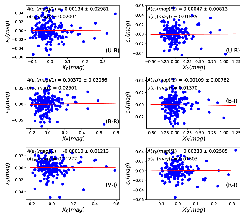
Figure 6: Correlation of residuals of colour differences (mag) $(e_{0},e_{2},e_{5},e_{6},e_{8},e_{9})$ with extinction after correcting the extinction formula with $R_{V}=2.25$. There are only four independent colours, meaning that the four extinction corrections allow us to cancel the correlations of all ten colours.

It seems unnatural to constrain the $\gamma_{ij}$ coefficients with $\chi^{2}_{\operatorname{Dex}}$, although they are (weakly) sensitive to the value of the extinction corrections. Our choice is instead to optimise the dispersion $\sigma(\gamma)$ displayed in Fig. 4, as stated in Sect. 5.3. At each value of the parameters ($\operatorname{Dex}_{F}$ or $\gamma_{i0}$), the $I_{i}$ and $X_{i}$ are obtained from Eq. 31, and the $\gamma_{i0}$ are retuned in order to minimise $\sigma(\gamma)$ in Fig. 4. This sequence is repeated four or five times to reach the final values of the seven unknown parameters (four $\operatorname{Dex}_{F}$ and three $\gamma_{i0}$). Within each cycle (extinction corrections $\operatorname{Dex}_{F}$ or $\gamma_{i0}$ fixed), convergence is reached when $\chi^{2}_{\operatorname{Dex}}$ or $\sigma(\gamma)$ increase whenever any one of the seven parameters is changed by $10^{-3}$. As the implemented model is still imperfect, the minima of $\chi^{2}_{\operatorname{Dex}}$ and $\sigma(\gamma)$ are not perfectly compatible; the differences between the two minima are nevertheless approximately ten times smaller than the quoted errors.

Table 8: Residual (mag) dependence on the extinction colour $R_{V}=2.25$ (after correction of the extinction formula). The corrections are introduced in Table 7 and the residuals are displayed in Fig. 6.

Index	Colour	$\textup{d}\epsilon/\textup{d}X_{3}$	Error ($\sigma$)	Residual ($\sigma$)	$\textup{d}\epsilon/\textup{d}X_{3}$
		no corr.	on slope (no corr.)	with corr.	with corr.
0	$U-B$	0.1138	0.0235	0.0201	$-0.0023$
1	$U-V$	0.0319	0.0059	0.0114	$-0.00127$
2	$U-R$	$-0.0498$	0.0054	0.0153	0.00400
3	$U-I$	0.0194	0.0029	0.0089	0.00021
4	$B-V$	$-0.0273$	0.0272	0.0294	0.00493
5	$B-R$	$-0.0995$	0.0125	0.0250	0.00915
6	$B-I$	$-0.0107$	0.0050	0.0137	$-0.00177$
7	$V-R$	$-0.2293$	0.0286	0.0248	0.02164
8	$V-I$	$-0.0079$	0.0086	0.0127	$-0.00035$
9	$R-I$	0.0370	0.0271	0.0150	0.01268

6 Quality of the colour reconstruction

The quality of the reconstruction of the colour differences $e_{i}$ from its intrinsic $I_{i}$ and extinction $X_{i}$ components is shown in Table 9 and in Fig. 7, where the distribution of the difference $\epsilon_{i}=c_{i}-(I_{i}+X_{i})$ is given for six selected colours. The average colour residual over the ten colours is 0.0176. As the colour measurement errors do not exceed 0.006, this figure (together with Table 9) suggests that the dominant contributions arise from modelling error and from the subtraction of the $\textup{ew}^{\textup{Si}}$ and $\textup{ew}^{\textup{Ca}}$ contributions. Given the accuracy reached, the phase of the spectrum might also contribute.

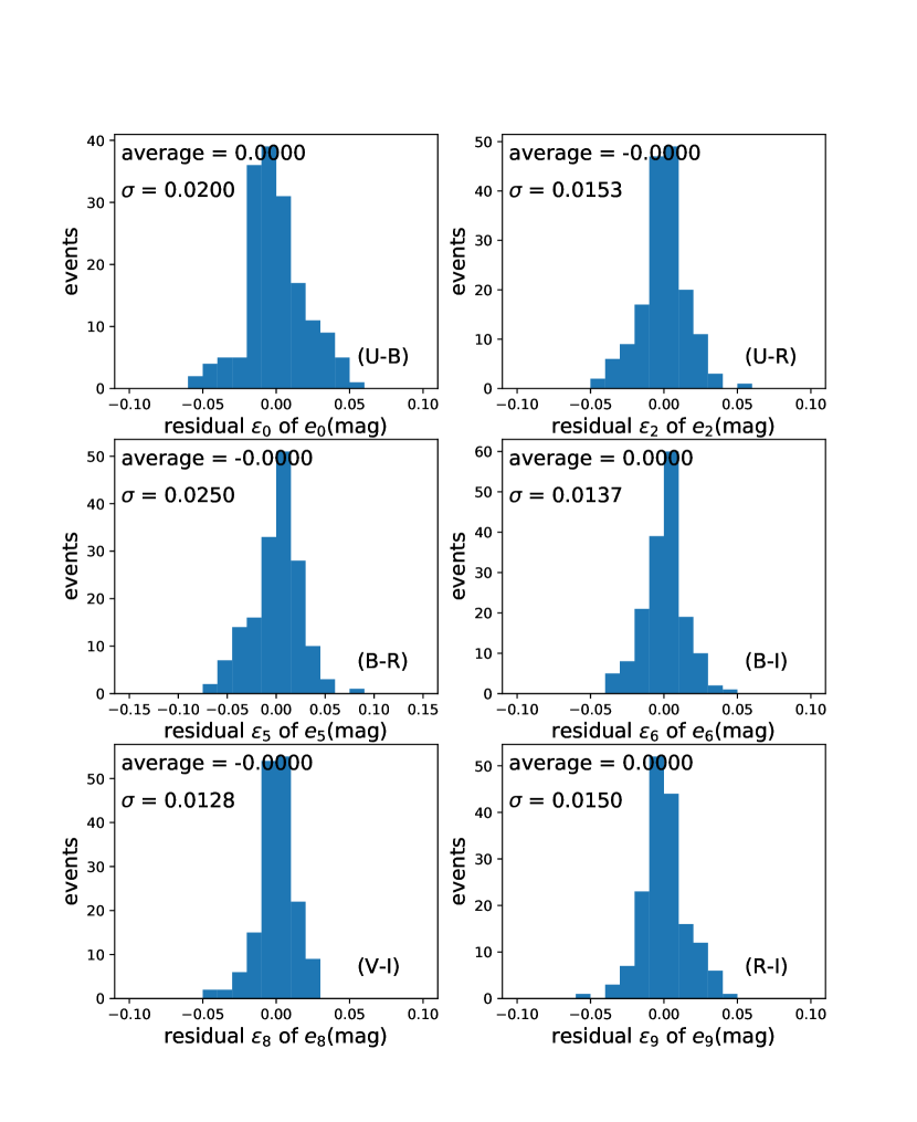
Figure 7: Residuals $\epsilon_{i}$ (mag) after the reconstruction of six colours $(c_{0},c_{2},c_{5},c_{6},c_{8},c_{9})$. The full list of residuals is given in Table 8.

7 Determination of $R_{V}$

7.1 Reddening correction of magnitudes

In Sect. 5.4, we ensure that the colour residuals are independent of the extinction component for each selected value of $R_{V}$. However, after correction for reddening, the magnitudes and the colours themselves may still depend on the extinction —even though the dependences in data and model must be the same after the corrections of Sect. 5.4. For each choice of $R_{V}$, the magnitude $m_{F}$ found from the data at a reference redshift of 0.05 is corrected for its dependence on $\textup{ew}^{\textup{Si}}$ and $\textup{ew}^{\textup{Ca}}$ —as carried out in Sect. 4.1 for colours— in order to obtain $m_{F}^{\textup{Ca}\textup{Si}}=m_{F}-\alpha_{\textup{Si}}\textup{ew}^{\textup{Si}}-\beta_{Ca}\textup{ew}^{\textup{Ca}}$. The dependence of $m_{F}^{\textup{Ca}\textup{Si}}$ on the intrinsic component $I_{i}$ with the (measured) coefficient $z_{F1}$ is then taken into account, and we allow for a single overall scaling factor $s(R_{V})$, which mimics the arbitrary $A_{V}$ used in most analyses (it should be unity in our framework) to define the extinction-corrected magnitude of each SN in the bandpass $F$ using colour $i$:

$$m_{F}^{\text{corr}}=m_{F}^{\textup{Ca}\textup{Si}}-z_{F1}I_{1}-s(R_{V})\,R_{F1}(R_{V})X_{1}.$$ (34)

Once the extinctions have been scaled according to Eq. 19, as explained in Sect. 4.2.2, the magnitude $m_{F}^{\text{corr}}$ should not depend on $X_{i}$. The extinction scale $s(R_{V})$ in Eq. 34 is chosen so as to cancel the dependence of the corrected data magnitude in the $V$ (top-hat) bandpass, and we expect $s(R_{V})=1$ for the physical value of $R_{V}$. It is seen in Fig. 8 that this is true when $R_{V}\approx 2.25$. The extinction in filter $F$ is now $A_{F}=s(R_{V})\times R_{F3}\times X_{3}$. However, if we turn to the other filters, we see in Fig. 9 that even after the extra scaling factor $s(\lambda)$ has been introduced in Eq. 34 to ensure $\textup{d}\text{mag}_{V}^{\text{corr}}/\textup{d}X_{3}=0$, the derivatives of the other bandpasses are finite when $R_{V}$ lies away from the $2.15-2.3$ range. The dependence of $\textup{d}m_{F}^{\text{corr}}/\textup{d}X_{3}$ as a function of $R_{V}$ is shown for the bandpasses $UBRI$ in Fig. 9. We find the extinction scale $s$ to be $s(R_{V}=2.20)=1.0269$ and $s(R_{V}=2.25)=1.0014$ (close to our ‘effective’ value of $R_{V}$). The errors in Figs. 8 to 11 are strongly correlated over the range of wavelengths, and for different values of $R_{V}$ as the same events are used. The error is evaluated from the dispersion of the scale factor in the ten samples of the simulation. From sample to sample, the scale parameter moves up and down in Fig. 8, but the smooth behaviour is preserved as a function of $R_{V}$ as the same events are involved for a given sample.

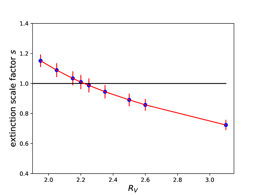
Figure 8: Extinction scale factor $s$ as a function of $R_{V}$ for $\textup{d}m_{V}/\textup{d}X_{3}=0$. For each value of $R_{V}$, there is a value of the extinction scale factor $s$ that cancels the dependence of the $V$ magnitude on extinction.

Each bandpass provides a value of the parameter $R_{V}$ that cancels the derivative $\textup{d}m_{F}^{\text{corr}}/\textup{d}X_{3}$. For $UBRI$, these values are respectively 2.283, 2.183, 2.137, and 2.240. We average the $U$ and $I$ measurements —which have a stronger $R_{V}$ dependence— and obtain (with the error from the simulation):

$$R_{V}=2.262\pm 0.126.$$ (35)

The scale factor $s$ for this value of $R_{V}$ is $s=1.001\pm 0.045$, which is additional independent confirmation of the result for $R_{V}$. We used magnitudes rather than colours to derive the previous result, but it can be reframed as a colour measurement: Figure 9 shows that the largest mismatch in the value of $\textup{d}m_{F}^{\text{corr}}/\textup{d}X_{3}$ is obtained by comparing the $U$ and $I$ bandpasses. We take advantage of this observation in Fig. 10 by imposing the condition that the derivative of the $U-I$ colour with respect to the extinction colour $X_{3}$ be zero after application of the extinction correction. The value of $R_{V}$ obtained in Fig. 10 is now $R_{V}=2.265$, which is almost the same as in Eq. 35, but the error is slightly smaller, as expected; the contributions from flux calibration error (0.03 mag), the redshift error, and the ‘grey’ fluctuation are suppressed. With this determination, the corresponding scale factor for the ‘extinction scale’ $s=1.000$. If we turn to the usual ‘operational’ definition of $R_{V}$, as $A_{V}/E(B-V)$, it is seen in Table 4 that $R_{V}=A_{V}/X_{4}=R_{V4}=2.7$. However, this numerical value is specific to SNe and our top-hat filters.

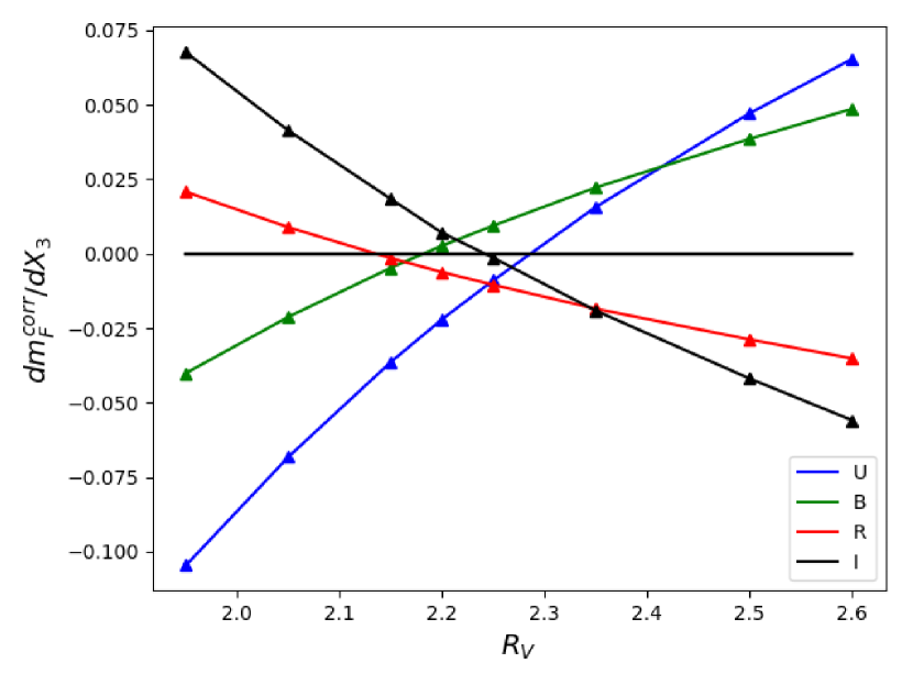
Figure 9: $\textup{d}m_{F}^{\text{corr}}/\textup{d}X_{3}$ for the $UBVRI$ bandpasses as a function of $R_{V}$. Although the dependence of the $V$ bandpasses as a function of extinction has been cancelled for each value of $R_{V}$, the extinction in other bandpasses is not adequately corrected.

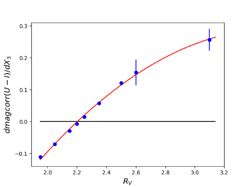
Figure 10: $\textup{d}(U-I)^{\text{corr}}/\textup{d}X_{3}$ as a function of $R_{V}$. The difference between $U$ and $I$ magnitudes (colour 3) is the most sensitive to the choice of $R_{V}$. The error bar is the dispersion found in the simulation.

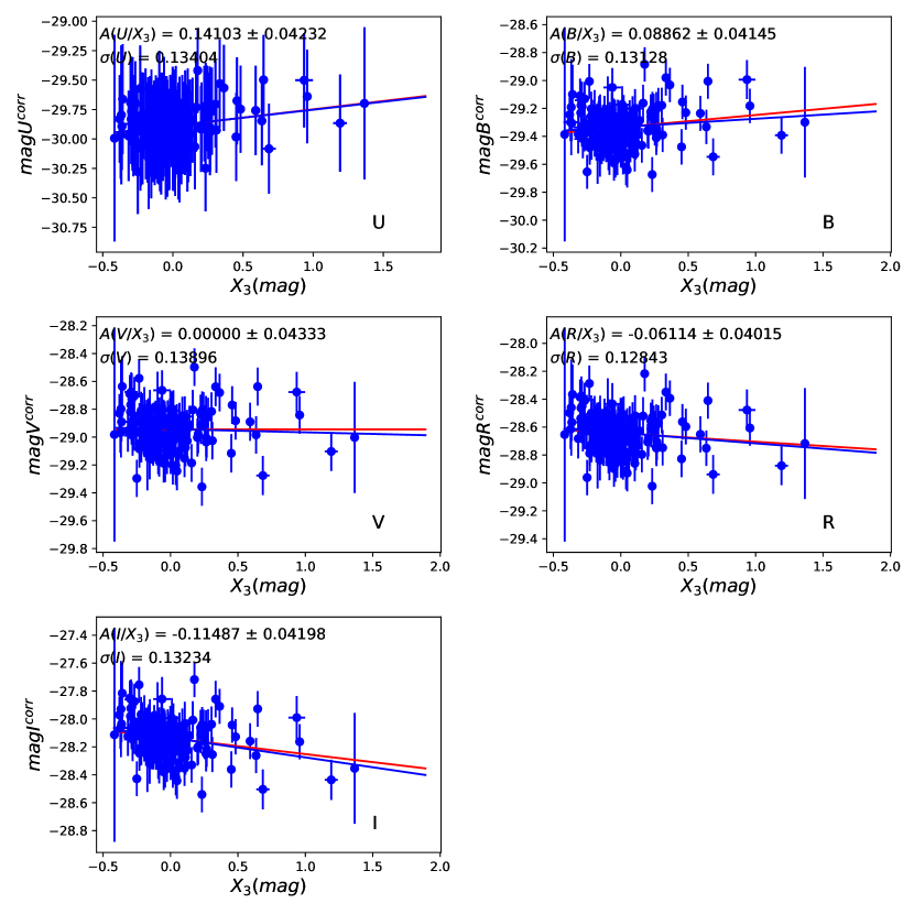
Figure 11: $UBVRI$ magnitudes corrected for $I_{3}$, $X_{3}$ with $R_{V}=3.100$, $s=0.73344$. The derivative $\textup{d}\text{mag}_{F}^{\text{corr}}/\textup{d}X_{3}$ is compatible with zero in each bandpass, but the variation from $U$ to $I$ is quite significant, taking correlations into account. The red line is weighted by errors and the blue straight line is unweighted.

The corrected magnitudes in the $UBVRI$ bandpasses are shown in Fig. 12 for the value $R_{V}=2.25$. As expected, no residual dependence of the (corrected) magnitude on the extinction is observed in any filter. The RMS (which was not minimised), has a value of 0.13 mag in all filters, which is smaller than the scatter of 0.15 mag typically seen in the SALT2 analyses of our sample (Saunders et al. 2018), but larger than the result from refined analyses designed to minimise this fluctuation, as in Boone et al. (2021). The blue straight line in Fig. 12 is a weighted fit and the red line is unweighted; the two slopes are almost identical. The magnitude fluctuation is ‘grey’, that is, it is almost identical over all bandpasses to a remarkable accuracy. For comparison, we show the magnitude correlations obtained for $R_{V}=3.1$ in Fig. 11. The scale factor must now be set to $s=0.857$ to ensure that the derivative $\textup{d}m^{\text{corr}}_{V}/\textup{d}X_{3}=0$. The error on the derivative of $\textup{d}(m_{U}-m_{I})/\textup{d}X_{3}$ in Fig. 10 is 0.04, as evaluated from the spread of the simulation samples, meaning that the significance of the rejection of $R_{V}=3.1$ (and higher) is actually 3.5 standard deviations.

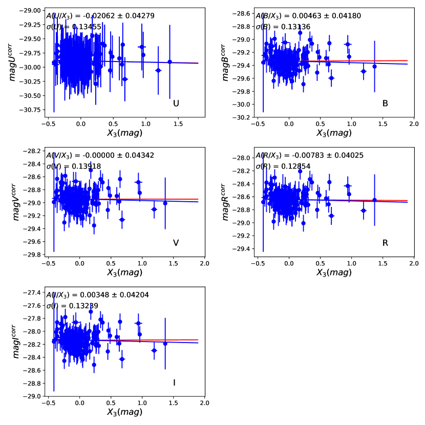
Figure 12: $UBVRI$ magnitudes corrected for $I_{3},X_{3}$ with $R_{V}=2.25$, $s=1.0024$. As for the previous figure, the red straight line is weighted by errors.

7.2 Deriving $R_{V}$ from the grey fluctuation

We mention in the previous section that the fluctuation of the magnitudes around the common ‘grey’ fluctuation of each SN Ia $i$, $m_{\text{grey}}(i)=\left(m_{U}^{\text{corr}}(i)+m_{B}^{\text{corr}}(i)+m_{V}^{\text{corr}}(i)+m_{R}^{\text{corr}}(i)+m_{I}^{\text{corr}}(i)\right)/5$, was remarkably small. This observation can be turned around and used to derive $R_{V}$: in each bandpass $F$, we compute the RMS $\sigma_{F}$ of the dispersion of the corrected magnitudes around $m_{\text{grey}}$. We show how this dispersion varies with $R_{V}$ in Fig. 13: a minimum is reached for $R_{V}=2.277$, which confirms the previous result. The dispersion in each $UBVRI$ bandpass with respect to the average offset over all filters is remarkably small, that is 0.0114, 0.0197, 0.0145, 0.0148, and 0.0060, respectively, which is everywhere smaller than 0.02. This result quantifies the level at which the remaining magnitude fluctuation is grey, and also confirms the validity of the modelling implemented (up to this ‘unaccounted’ grey fluctuation).

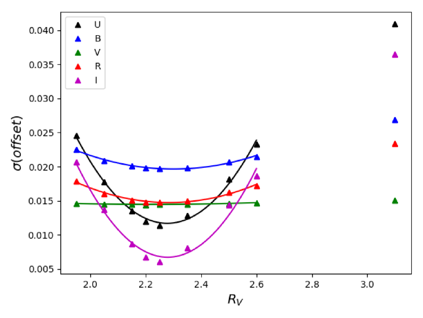
Figure 13: RMS of the offsets (with respect to $m_{\text{grey}}$) of the corrected $UBVRI$ magnitudes as a function of $R_{V}$.

8 Simulation

The previous results can be summarised by ten numbers: the five extinction corrections to the extinction formula in the five bandpasses used for our analysis, the three intrinsic colour ratios, the extinction scale $s$, and the extinction parameter $R_{V}$. These are the ‘effective’ values found within our algorithms, but not necessarily the ‘true’ values. The biases and the errors are evaluated below based on a simulation that mimics the observations. We use the values of the parameters tuned to describe the data to generate the events, and then proceed with the same analysis. The differences from the reconstructed values allow us to find the methodological biases, and the scatter among the different generated samples helps us find the statistical error.

8.1 Generation of colours with their error

We generate nine samples of 165 SNe Ia $UBVRI$ magnitudes. The generated intrinsic $I^{g}_{1}$ and extinction $X^{g}_{1}$ components of colour $1\equiv U-V$ follow the observed distribution in the data after smoothing by a sliding local averaging (to avoid counting the statistical fluctuations twice): in each histogram bin, the data distribution of $I_{1}$ and $X_{1}$ was replaced by the average of three adjacent bins. Whenever the bin statistics was below four events, the average of five bins was used. The other intrinsic colours $I^{g}_{k}$ obey $I^{g}_{k}=\gamma_{k1}I^{g}_{1}$, and the extinction colours $X^{g}_{k}$ follow from $X^{g}_{k}=\delta_{k1}X^{g}_{1}$. The coefficients $\delta_{ij}$ used in the generation are the ones found in the data analysis; that is, they include the correction to the FM99 formula described in Table 7. The simulation shows that the analysis does recover the input corrections, with a small bias. As the measurement errors are included in the observed data distribution, they should have been removed from the generation in the simulation. We instead introduced a single simulation scaling factor of the $I^{g}_{1}$ distribution, tuned so that the reconstructed intrinsic components should match the observations once the analysis is applied; it depends on the simulated sample, but its difference from unity never exceeds 0.01. This effect is expected to be smaller for the extinction colours $X_{i}$, which have a larger range, and the observed distribution of the data has been used.

8.2 Colour noise

The noise is derived from the residuals observed in the data, and it combines measurement and modelling errors. The residuals $\epsilon_{i}$ measured from the data in four colours (i.e. $2\equiv U-R$, $5\equiv B-R$, $7\equiv V-R$, $9\equiv R-I$) are used to derive a $4\times 4$ covariance matrix $\langle\epsilon_{i}\epsilon_{j}\rangle$. The square roots of the dominant eigenvalues are $\sigma_{1}=0.026525$, $\sigma_{2}=0.017947$; the other eigenvalues are negligible ($\sim 10^{-4}$ and $\sim 3\,10^{-5}$). The Gaussian noise of the two eigenvectors is then projected onto the four bandpasses to obtain a simulated ‘colour noise’ for the four colours. We find that this noise has to be multiplied by 1.004 in the simulation to reproduce the observed residuals. This effect may arise from the contribution of modelling errors to the data, while the model is exact in the simulation.

8.3 Generation of magnitudes

The $R$ magnitude is used as the reference. A correction reproducing its (small) correlation with the intrinsic colour is added. The magnitudes in the $UBVI$ bandpasses are obtained by adding the $U-R$, $B-R$, $V-R$, and $I-R$ colours, as found from their intrinsic and extinction components, and including the ‘colour noise’. Finally, a Gaussian grey magnitude fluctuation with $\sigma(grey)=0.12$ is added, though its value is irrelevant for all the results of the present study. The generated magnitudes of event $n$ in bandpass $R$ and $U$ are therefore described as

$$m_{R}(n) =z_{R1}I_{1}(n)+R_{R1}X_{1}(n)+\text{grey}(n),$$ (36)

$$m_{U}(n) =m_{R}(n)+\gamma_{21}I_{1}(n)+\delta_{21}X_{1}(n)+\sigma_{1}u_{1}(n)\,n_{21}+\sigma_{2}u_{2}(n)\,n_{22},$$ (37)

where $u_{1}(n)$ and $u_{2}(n)$ are centred random Gaussian variables with a standard deviation of unity, $n_{21}$ and $n_{22}$ are the components of the corresponding eigenvectors on the $U-R$ colour, and $z_{R1}$ is the observed correlation between the $R$ magnitude and the intrinsic colour 1. The generated magnitudes are processed by the same algorithms as the data (after $\textup{ew}^{\textup{Ca}}$ and $\textup{ew}^{\textup{Si}}$ corrections), providing reconstructed values for $I_{i}$ and $X_{i}$, reconstructed extinction corrections, reconstructed intrinsic couplings, and a reconstructed $R_{V}$.

8.4 Simulated and observed distributions

As we want to evaluate the errors and biases of the data analysis, with the help of the simulation, both the distributions and the errors must be similar in the observations and the simulation. The $(I_{i},X_{i})$ obtained through the colour analysis (as in the data), and the generated $(I^{g}_{i},X^{g}_{i})$ values are compared for three colours in Fig. 14 for the simulated sample 1 and in Table 9. There is a very small scatter between the generated and reconstructed colour components, and their ratio is close to unity. This scatter varies from 0.002 to 0.006 for $I_{i}$, and from 0.001 to 0.006 for $X_{i}$. The systematic trend in the ratio of measured and generated colour is partially statistical and fluctuates from one sample to another in a range of 0.02, which justifies using the observed distributions as an input for the simulation. The scatter in Fig. 14 is surprisingly smaller than the RMS of the observed residuals (in average 0.0176 mag). This is a consequence of the averaging over different colours performed in Eq. 31. The simulated accuracy is tuned to reproduce the observed residuals by the introduction of two ad hoc factors in the noise and the rescaling of the distribution of $I_{1}$ (of colour $U-V$) used in the generation. The distribution of the residuals is shown in Fig. 16 and Table 9.

Figure 14: Comparison of intrinsic and extinction components (mag) in generation and reconstruction for colours $c_{0}$, $c_{5}$, and $c_{9}$. The small differences found justify using the (smoothed) observed distributions of $I_{1}$ and $X_{1}$ as input.

For the same three colours ($c_{0}$, $c_{5}$, $c_{9}$), the intrinsic and extinction colour distributions for the data and one of the simulated samples are shown in Fig. 15. The results for all colours are summarised in Table 9. The residuals in the data and the simulation are compared in Fig. 16 and Table 9. The intrinsic and extinction colours in the simulation and observation agree, and the trends of the errors are also well reproduced by the simulation.

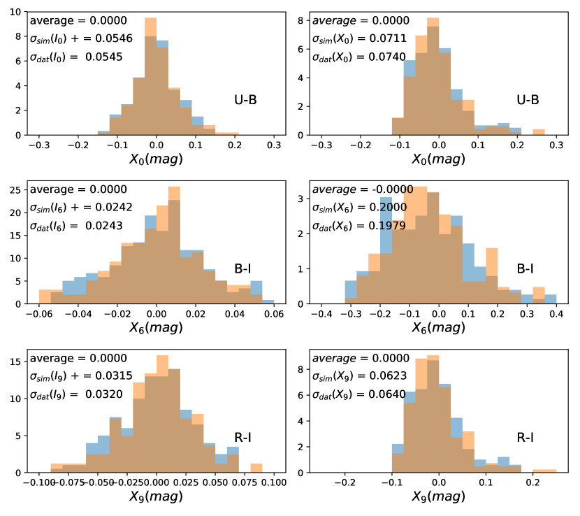
Figure 15: Distributions of intrinsic and extinction components of $c_{0}$, $c_{6}$, and $c_{9}$ in observation and simulation for $R_{V}=2.25$ (mag). The extinction is asymmetric, with an extended tail to high values. The intrinsic part is symmetric. The RMS for all colours is given in Table 9. The blue shade is the simulated distribution, the orange shade the data.

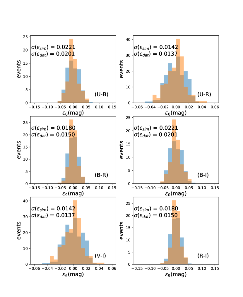
Figure 16: Residuals in observations and simulations for colours $c_{0}$, $c_{2}$, $c_{5}$, $c_{6}$, $c_{8}$, and $c_{9}$ ($R_{V}=2.25$). The RMS of the residuals of all colours are given in Table 9. The blue shade is the simulated distribution, the orange shade the data.

Table 9: Range of the intrinsic and extinction colours for observation, simulation (seed2), and residuals (mag).

Index	Colour	$\sigma(I_{i})$	$\sigma(I_{i})$	$\sigma(X_{i})$	$\sigma(X_{i})$	$\sigma(\epsilon_{i})$	$\sigma(\epsilon_{i})$
		Sim (mag)	Obs (mag)	Sim (mag)	Obs (mag)	Sim (mag)	Obs (mag)
0	$U-B$	0.0544	0.0545	0.0681	0.0740	0.0216	0.0201
1	$U-V$	0.0701	0.0692	0.1473	0.1560	0.0084	0.0114
2	$U-R$	0.0625	0.0610	0.1996	0.2080	0.0169	0.0154
3	$U-I$	0.0303	0.0304	0.2684	0.2719	0.0097	0.0089
4	$B-V$	0.0149	0.0152	0.0791	0.0818	0.0250	0.0295
5	$B-R$	0.0060	0.0069	0.1316	0.1339	0.0300	0.0250
6	$B-I$	0.0239	0.0243	0.2003	0.1979	0.0141	0.0137
7	$V-R$	0.0082	0.0082	0.0524	0.0519	0.0230	0.0248
8	$V-I$	0.0390	0.0401	0.1210	0.1160	0.0094	0.0127
9	$R-I$	0.0296	0.0320	0.0686	0.0640	0.0178	0.0150

8.5 Errors on the extinction formula corrections

We rely on the nine simulated samples to control the bias in the measurements arising from the implemented algorithms, as well as the errors on the extracted parameters: extinction corrections $\operatorname{Dex}_{F}$, the value of $R_{V}$, and the extinction scale $s_{X}$. The analysis was performed on each of the samples, on the same grid of values of $R_{V}$. The mean value of the reconstructed extinction corrections and their dispersion is given in Table 10.

Table 10: Extinction correction for $R_{V}=2.25$.

Filter	$\operatorname{Dex}_{F}$ obs	$\operatorname{Dex}_{F}$ sim	bias	$\sigma(\operatorname{Dex}_{F})$	$\operatorname{Dex}_{F}$ final
	(= generation, mag)	(average, mag)	(average, mag)	(mag)	(mag)
$U$	$0.0675$	$0.0675$	$0.0$	$0.0$	$0.0675$
$B$	$-0.0415$	$-0.0351$	$0.0064$	$0.0168$	$-0.0479$
$V$	$-0.0435$	$-0.0433$	$0.0002$	$0.0120$	$-0.0437$
$R$	$0.1015$	$0.0733$	$-0.0282$	$0.0342$	$0.1297$
$I$	$-0.1109$	$-0.1390$	$0.0280$	$0.0498$	$-0.0829$

When comparing to Table 4, it is seen that the corrections to the extinction are statistically significant, rising from 1 to 10 percent over the visible spectrum once the bias is taken into account. The algorithm used in deriving the corrections is able to extract their value, with some biases. Accepting the biases found in the simulation, our final values for the corrections to the extinction coefficients are given in the last column of Table 10 for $R_{V}=2.25$. The error on the bias correction is $\sigma(\operatorname{Dex}_{F})/3$ as nine samples are generated.

8.6 Errors on the intrinsic coupling coefficients $\gamma$

For each simulation sample and each value of $R_{V}$ in the grid, the three intrinsic coupling coefficients $\gamma_{10}$, $\gamma_{20}$, and $\gamma_{30}$, are evaluated as in the data analysis, that is by minimising the scatter in the plot comparing the input values to the results. The standard deviation of the three coefficients from one sample to the next is respectively 0.0075, 0.0061, and 0.0041. The values averaged over all samples allow us to estimate the bias arising from the analysis; it is found to be of the same order as the statistical error. The largest contribution to the error is by far the one discussed in Sect. 5.1, which arises from different choices of auxiliary colours, and is given in Table 6. The statistical error will be added into the final uncertainty.

8.7 Errors on the extinction parameter $R_{V}$

The measurement of $R_{V}$ is also performed on the simulation. The value in the generation was $R_{V}=2.20$, and the average value found is $R_{V}=2.284\pm 0.112$. We correct the result obtained in the data analysis, of 2.265, to $R_{V}=2.265-0.084=2.181\pm 0.117$ (the error is increased to account for the uncertainty on the bias correction). As the values found in the four filters $BVRI$ are almost fully correlated, we use the error on $R_{V}$ derived from the $U-I$ colour. We add the impact of an estimated systematic error in the measurement of colours and other corrections (earth atmosphere, galactic extinction, host galaxy subtraction, silicon and calcium contribution). As we only use differences between mean and measured colours, many instrumental systematic errors cancel out. To evaluate the impact on $R_{V}$, all colours were modified by a shift proportional to their value and reaching 0.005 mag over their range of variation. The outcome is a change in $R_{V}$ by 0.05. The final result for the parameter $R_{V}$ (including the error on the bias) is then

$$R_{V}=2.181\pm 0.117\;(\text{stat.})\pm 0.050\;(\text{syst.}).$$ (38)

9 No calcium or silicon line corrections

We tried to reproduce our analysis without performing the initial correction for the $\textup{ew}^{\textup{Si}}$ and $\textup{ew}^{\textup{Ca}}$ spectral lines. The intrinsic colours are expected to be much larger than in the previous analysis. They reach 0.10 in colours ($U-B$, $U-V$, $U-R$). The mean colour residual is then 0.0402 (instead of 0.0176 with the colour corrections from $\textup{ew}^{\textup{Ca}}$ and $\textup{ew}^{\textup{Si}}$). The square roots of the dominant eigenvalues of the covariance matrix from the residuals are 0.0724 and 0.0296, meaning that it would be necessary to add two spectral coordinates for each SN in order to reduce these residuals, instead of tolerating these contributions as ‘noise’ as is done in the present work. The two eigenvectors are $(0.5842,0.5974,0.4373,-0.3324)$ and $(0.5972,-0.7405,0.2908,0.1013)$. In the absence of $\textup{ew}^{\textup{Si}}$ and $\textup{ew}^{\textup{Ca}}$ corrections, the model we used fails to describe the observations, as we are missing key spectral information. Instead, the approach we take is to add back the colour contributions of Si II $\lambda$4131 and Ca II H&K $\lambda$3945 —which are subtracted in Sect. 4.1— to obtain a ‘full’ intrinsic component of colour variability; this is shown in Fig. 17.

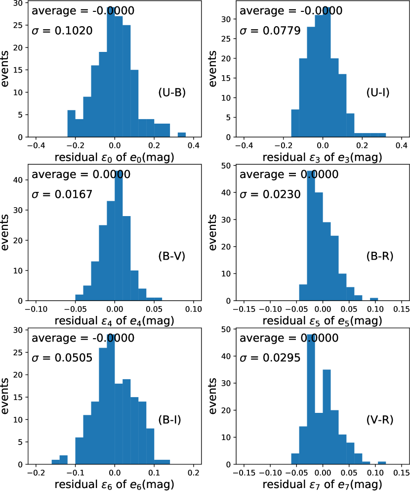
Figure 17: Distributions of six ‘full’ intrinsic colours including Si II and Ca II H&K contributions.

The range of the full intrinsic colour component is given in Table 11 for all colours. The small size of the intrinsic part of $e_{4}\equiv B-V$ justifies using it as a simplified indicator of extinction for SNe Ia.

Table 11: Range of the full intrinsic colour component and correlations between the full calcium–silicon colour correction DCaSi and the SALT $x_{1}$ variable ($R_{V}=2.25$).

Index	colour	$\sigma_{\text{full}}$	$\textup{d}\textup{DCaSi}/\textup{d}x_{1}$	$\sigma(\textup{DCaSi})$
0	$U-B$	0.1020	$-0.0300$	0.0808
1	$U-V$	0.1088	$-0.0246$	0.0802
2	$U-R$	0.1170	$-0.0482$	0.0873
3	$U-I$	0.0780	$-0.0495$	0.0518
4	$B-V$	0.016	0.0054	0.0035
5	$B-R$	0.0230	$-0.0182$	0.0121
6	$B-I$	0.0505	$-0.0194$	0.0397
7	$V-R$	0.0295	$-0.0235$	0.0155
8	$V-I$	0.0627	$-0.0248$	0.0411
9	$R-I$	0.0519	$-0.0013$	0.0407

The standard choice of colour $4\equiv B-V$ as an extinction indicator is fortunate, as the intrinsic content happens to be small. However, a large part of the calcium and silicon correction can be recovered, with information extracted from the light curve. The SALT2 stretch variable $x_{1}$, as described in Betoule et al. (2014), is strongly correlated to the combined calcium–silicon corrections $\textup{DCaSi}(i)=\sigma_{i}\textup{ew}^{\textup{Si}}+\kappa_{i}\textup{ew}^{\textup{$\textup{Ca}$}}$, as shown in Fig. 18 and in Table 11 for all colours. The dispersion of the full intrinsic colour can be compared to the results of previous determinations: $\sigma_{BV}^{\text{int}}=0.049$ (Jha et al. 2007), $\sigma_{BV}^{\text{int}}=0.03\pm 0.01$; $\sigma_{VR}^{\text{int}}=0.04\pm 0.01$, $\sigma_{RI}^{\text{int}}=0.06\pm 0.01$ (Nobili & Goobar 2008), $\sigma_{BV}^{\text{int}}=0.065\pm 0.008$ (Mandel et al. 2017), $\sigma_{BV}^{\text{int1}}=0.076\pm 0.011$, $\sigma_{BV}^{\text{int2}}=0.043\pm 0.013$ (2populations/decline rate, Wojtak et al. 2023). The values of $\sigma_{BV}^{\text{int}}$ found in this work for the two populations of the $H_{\alpha}$ subsample (galaxies with high and low $H_{\alpha}$ signal, as discussed in item 10 of Sect. 10) are: $\sigma_{BV}^{\text{int1}}=0.0127$, $\sigma_{BV}^{\text{int2}}=0.0149$.

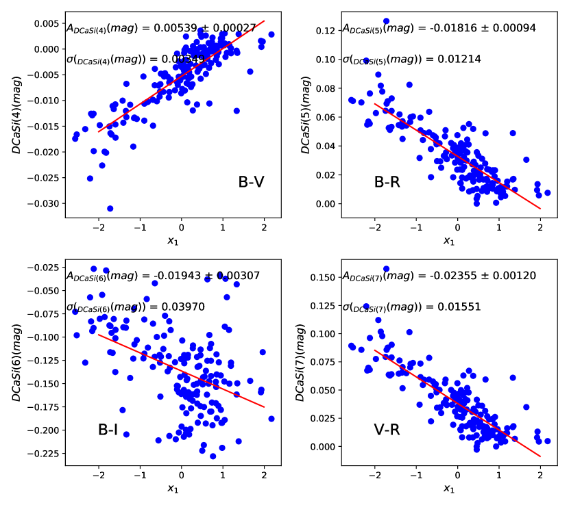
Figure 18: Correlations between the combined calcium–silicon correction DCaSi and the SALT2 variable $x_{1}$ for four colours.

The smallest scatter of DCaSi is found for colour $4\equiv B-V$, with $\sigma=0.00349$. This provides an estimate of the contribution of measurement errors to colours, all colours being processed in the same way. Extra physical variabilities worsen the evaluation of the DCaSi contribution of other colours.

10 Conclusions

The focus of this work is the extraction for each SN of our sample of extinction and intrinsic colour components, using the extinction formula for dust in our galaxy as leverage. This colour analysis is well adapted to the determination of the reddening, but does not make use of the full power of the spectral information for the intrinsic part. The linearity that we find in the correlations between different colours is nevertheless an interesting feature by itself.

1. The model presented in this work assumes the factorisation of the extinction by the host galaxy, without any correlation with the intrinsic properties of the SN. We acknowledge that the presence of circumstellar dust might invalidate this assumption.

2. The modelling of colour fluctuations requires the inclusion of four corrections to the extinction formula in the $BVRI$ bandpasses, three intrinsic coefficients correlating the different colours, and one value for $R_{V}$. An additional scale parameter for the extinction should be set to unity. The colour accuracy achieved varies from 0.011 to 0.028 mag depending on the colour. All colours discussed in this work are ‘rest-frame’ colours. Such corrections could arise from different average dust contents in host galaxies and ours. One of the assumptions of the model (factorisation of the extinction, linearity of the correlations of intrinsic colours) could be wrong, though plausible, but we are surprised by the large difference found in the corrections to the R and I bandpasses $\operatorname{Dex}_{R}$ and $\operatorname{Dex}_{I}$ shown in Table 4 and observed directly in Fig. 5. The simulation confirms that the algorithm we use is indeed sensitive to these small corrections. The errors arising from the linear approximation cannot account for the size of the effects found, and additional intrinsic contributions are extremely unlikely to induce a correlation with extinction as strong as the one observed in Fig. 5.

3. A single extra-intrinsic contribution beyond Si II $\lambda$4131 Åand Ca II H&K $\lambda$3945 Å is needed to account for the colour correlations within the accuracy described immediately above We can then extract intrinsic and extinction colour components for each SN.

4. We show that the remaining magnitude fluctuation of 0.13 mag is independent of the five $UBVRI$ bandpasses to an accuracy of better than 0.02 mag, reaching 0.007 mag for the $I$ bandpass. There is no attempt to minimise this magnitude dispersion directly in our procedure.

5. When the extinction formula of FM99 is used as leverage to extract this extra intrinsic (one-dimensional) component, and the associated extinction component, the intrinsic coupling coefficients between the different colours are consistent over the full sample of SNe Ia at the level of 0.01–0.05. The values of the three independent coefficients are (for $R_{V}=2.25$)

   $$\begin{gathered}\gamma_{10}=1.265\pm 0.075,\\ \gamma_{20}=1.116\pm 0.061,\\ \gamma_{30}=0.539\pm 0.041.\end{gathered}$$ (39)

   The errors quoted include the systematic errors from the colour choice, and the statistical error derived from the simulation. The extra ‘intrinsic’ content of $U-I$ is half the size of $U-B$ or $U-V$, with a large uncertainty.

6. After correcting for the analysis bias found in the simulation, the optimal mean value of the FM99 parameter $R_{V}$ over our sample is found to be

   $$R_{V}=2.218\pm 0.117\;(\text{stat.})\pm 0.050\;(\text{syst.}).$$ (40)

   This value is obtained within our specific treatment of the extinction scale, which is not universally adopted. The usual ‘operational’ definition $R_{V}=A_{V}/E(B-V)=R_{V4}$ then leads to $R_{V4}=2.7$ according to Table 4, which includes the effect of our different filter definition.

7. The associated scaling factor for the extinction component is measured to be $1.001\pm 0.044$, and, as desired for consistency, is compatible with unity.

8. A previous SNfactory analysis in C11 found $R_{V}=2.8\pm 0.30$, with a different method and a substantially different data set. A few improvements are brought here, namely the rescaling of the extinction coefficients, ensuring consistency with the $B$ and $V$ SN spectra; the presence of an ‘extra-intrinsic’ colour component; and we avoid an arbitrary extinction parameter for each SN ($A_{V}$). The presence of the grey fluctuation was ignored by C11, and the extraction of the extinction colour component was not explicit. The $R_{V}$ value that we obtain is dependent on the method used, with an emphasis on colour correlations rather than a minimisation of Hubble residuals. The smaller number of parameters involved and the accuracy of the colour description is an argument in favour of the present method.

9. Within the accuracy of the present observations, we see no hint of a variation of the parameter $R_{V}$ from one SN to another. As we find corrections to the extinction formula to be necessary, for all values of $R_{V}$ in the range 1.95 to 2.60, the meaning of this parameter is slightly blurred. Simulations have been performed with samples including a Gaussian distribution of the value of $R_{V}$ around the value of 2.20 and with an RMS of 0.5. The results do not show any significant change, and we would thus be insensitive to such a fluctuation.

10. Many instances have been given in the past of a correlation between the star formation rate (H$\alpha$ signal, Rigault et al. 2013) or the host galaxy mass (Hamuy et al. 2000; Kelly et al. 2010) and the absolute magnitudes of SNe, as well as their intrinsic properties, suggesting two populations depending on their age. We checked the impact on our analysis of including a sample of 85 SNe from the SNfactory collaboration common to the Rigault et al. (2013) sample. A striking difference is seen in the amount of extinction of the two groups. The young SNe (high H$\alpha$ signal of the host galaxy) have significantly more dust, with $\langle X_{3}\rangle=0.0124\pm 0.036$, whilst the older ones (low galactic H$\alpha$ signal) have less extinction and $\langle X_{3}\rangle=-0.0577\pm 0.025$. Our corrections slightly reduce the discrepancy in absolute magnitude of the two samples from 0.095 to 0.087 mag. The statistics of the two groups (47 and 37 SNe) are too small to evaluate a difference in the associated $R_{V}$.

The colour model used here achieves an impressive level of accuracy in the description of the ’grey’ magnitude fluctuation, which may help interpret the effect. The accuracy reached on the (smaller) intrinsic colour might be improved by using additional spectral information, in particular Si II $\lambda$6355 Å, which is better measured. This will require dealing with the additional complexity arising from non-linear effects.

Appendix A Linearisation of the extinction formula

The observed photon-count distribution was given in Eq. 11 where the function $\phi(\lambda)$ is provided by Cardelli et al. (1989); O’Donnell (1994); Fitzpatrick (1999); Fitzpatrick & Massa (2005). To simplify the computations, we assume the extinction $E(B-V)$ is small enough to allow a linear approximation under the exponentiation.

$$10^{-0.4\phi(\lambda,R_{V})\,E(B-V)}\approx 1-0.4\ln 10\,\phi(\lambda,R_{V})\,E(B-V).$$ (41)

We define $A(\lambda,R_{V})=\phi(\lambda,R_{V})\,E(B-V)$, the observed spectrum (photon counts) is then

$$m(\lambda)=-2.5\log_{10}s(\lambda)=-2.5\log_{10}s_{0}(\lambda)+A(\lambda,R_{V}).$$ (42)

When the unextincted SN spectrum $s_{0}(\lambda)$ is integrated over a spectral band, such as $B$, with transmission $T(\lambda)$, the rest frame flux is:

$$s_{B}=\int_{B}s_{0}(\lambda)T(\lambda)\,10^{-0.4\,\phi(\lambda)}\textup{d}\lambda.$$ (43)

In our synthetic photometry, unit-transmission top-hat filters are used, and so we omit $T(\lambda)$. Using the previous linear approximation:

$$m_{B}^{\text{obs}} =m_{B}^{\text{true}}+A_{B}$$

$$=-2.5\log_{10}\left(\int_{B}s_{0}(\lambda)\left[1-0.4\ln 10\,A(\lambda,R_{V})\right]\textup{d}\lambda\right).$$ (44)

The logarithm can be expanded to give

$$A_{B}=m_{B}^{\text{obs}}-m_{B}^{\text{true}}=\frac{\int_{B}s_{0}(\lambda)A(\lambda,R_{V})\,\textup{d}\lambda}{\int_{B}s_{0}(\lambda)\,\textup{d}\lambda}.$$ (45)

In this approximation, the extinction is simply weighted by the spectrum over the filter bandpass. The maximal value of the extinction component $X_{4}$ is 0.4, and the error $\delta R_{F4}=R_{F4}^{\text{linear}}-R_{F4}^{\text{exact}}$ arising from the linear approximation in the evaluation of the extinctions coefficient $R_{F4}$ in the different (top-hat) filters is given in Table 12. The magnitude correction is obtained by multiplying the coefficients $R_{F4}$ by $X_{4}$, and so the error on this correction never exceeds 0.005 mag, and cannot account for the effects observed in Fig. 5.

Table 12: Error on the bandpass extinction coefficients arising from the linear approximation for $X_{4}=0.4$

. Filter $U$ $B$ $V$ $R$ $I$ $\delta R^{\prime}_{F4}$ $-0.00976$ $-0.00870$ $-0.01147$ $-0.00494$ $-0.00195$