Sparsity-Aware Distributed Learning for Gaussian Processes with Linear Multiple Kernel

Abstract

Gaussian processes (GPs) stand as crucial tools in machine learning and signal processing, with their effectiveness hinging on kernel design and hyper-parameter optimization. This paper presents a novel GP linear multiple kernel (LMK) and a generic sparsity-aware distributed learning framework to optimize the hyper-parameters. The newly proposed grid spectral mixture (GSM) kernel is tailored for multi-dimensional data, effectively reducing the number of hyper-parameters while maintaining good approximation capabilities. We further demonstrate that the associated hyper-parameter optimization of this kernel yields sparse solutions. To exploit the inherent sparsity property of the solutions, we introduce the Sparse LInear Multiple Kernel Learning (SLIM-KL) framework. The framework incorporates a quantized alternating direction method of multipliers (ADMM) scheme for collaborative learning among multiple agents, where the local optimization problem is solved using a distributed successive convex approximation (DSCA) algorithm. SLIM-KL effectively manages large-scale hyper-parameter optimization for the proposed kernel, simultaneously ensuring data privacy and minimizing communication costs. Theoretical analysis establishes convergence guarantees for the learning framework, while experiments on diverse datasets demonstrate the superior prediction performance and efficiency of our proposed methods.

I Introduction

Recently, Bayesian methods have gained significant attention across a wide range of machine learning and signal processing applications. They are known for their ability to enhance model robustness by leveraging prior knowledge and effectively handling uncertainties associated with parameter estimates [1]. Among these methods, Gaussian process (GP) has emerged as a particularly promising model that offers reliable estimates accompanied by uncertainty quantification [2, 3]. The distinctive strength of GP lies in its explicit modeling of the underlying function using a GP prior, which empowers GP to capture intricate patterns in the data, even with limited observations [4, 5]. Unlike conventional machine learning models that rely on point estimates, GP embraces a probabilistic framework that yields a posterior distribution over the function given the observed data [6, 7].

The representation power of a GP model heavily relies on the selection of an appropriate kernel function. Several traditional kernel functions have been used in GP models, including the squared-exponential (SE) kernel, Ornstein-Uhlenbeck kernel, rational quadratic kernel, and periodic kernel, among others [2]. These kernel functions can even be combined, for example, into a linear multiple kernel (LMK) in the form of a linearly-weighted sum to enhance the overall modeling capacity [8]. However, the selection of these preliminary kernel functions often relies heavily on subjective expert knowledge, making it impractical for complex applications.

To address the challenge of manual kernel design, Wilson et al. proposed the spectral mixture (SM) kernel to discover underlying data patterns automatically via formulating the spectral density of kernel as a Gaussian mixture [9]. However, the original SM kernel presents difficulties in tuning its hyper-parameters due to the non-convex nature of the optimization problem. This increases the risk of getting stuck at a sub-optimal solution, especially when dealing with a large number of hyper-parameters. The grid spectral mixture (GSM) kernel was proposed to address this drawback in the SM kernel [10]. Specifically, the GSM kernel focuses on optimizing the weights of each kernel component while fixing other hyper-parameters, resulting to a more favorable optimization structure. Consequently, the GSM kernel acts as a LMK, allowing its sub-kernels to exhibit beneficial low-rank properties under reasonable conditions [10]. By identifying a sparse subset of the most relevant frequency components in the input data, the GSM kernel enhances the GP model interpretability and facilitates a clearer understanding of the underlying data patterns.

While leveraging GSM kernel-based GP (GSMGP) models holds great potential [11], it also comes with several challenges. The existing formulation of the GSM kernel is only suitable for handling one-dimensional data [10], and naively extending it to multi-dimensional data leads to potential issues, as the number of hyper-parameters and the model complexity increase exponentially with the dimensions [12]. Additionally, centralized optimization of the GSMGP models in real-world scenarios introduces further challenges. On one hand, the $\mathcal{O}(n^{3})$ computational complexity, where $n$ is the training data size, hinders the scalability of GSMGP in big data applications [13, 14]. On the other hand, collecting data centrally becomes difficult in practice, as data are often distributed across locations or devices, and concerns about data privacy often discourage individual data owners from sharing their data [15].

In this paper, we focus on addressing such challenges associated with GSMGP models. The main contributions of this paper are summarized as follows:

• We introduce a novel formulation for the GSM kernel capable of accommodating multi-dimensional data. Compared to existing formulations [10, 11, 12], our approach effectively reduces the number of hyper-parameters while maintaining a good approximation capability. Furthermore, the proposed kernel exhibits a sparsity-promoting property that enables efficient optimization of the hyper-parameters.

• By exploiting the inherent sparsity of the proposed kernel, we introduce a sparsity-aware distributed learning framework for GPs with LMK, termed Sparse LInear Multiple Kernel Learning (SLIM-KL), which consists of two main components: 1) A quantized alternating direction method of multipliers (ADMM) scheme, allowing multiple agents to collaboratively learn the kernel hyper-parameters while preserving data privacy and reducing communication costs; and 2) a distributed successive convex approximation (DSCA) algorithm for solving the local hyper-parameter optimization problem in a distributed manner within the quantized ADMM. As a result, SLIM-KL offers scalability, maintains privacy, and ensures efficient communication.

• We provide a comprehensive theoretical analysis for the proposed learning framework. Additionally, we conduct extensive experiments on diverse one-dimensional and multi-dimensional datasets to evaluate its performance. The results demonstrate that our proposed framework consistently outperform the existing approaches in terms of prediction performance and efficiency.

The remainder of this paper is organized as follows. Section II reviews the GP regression and GSM kernel. Sections III and IV introduce the proposed kernel formulation and learning framework. Section V presents the theoretical analysis of our proposed framework. Section VI demonstrates the experimental results. Finally, Section VII concludes the paper. Key technical proofs and derivations are given in the Appendix.

II Preliminaries

This section firstly reviews the classical GP regression. Then, the GSM kernel and the associated hyper-parameter optimization are introduced.

II-A Gaussian Process Regression

By definition, Gaussian process (GP) is a collection of random variables, any finite number of which have a joint Gaussian distribution [2]. Mathematically, a real-valued, scalar GP $f(\bm{x})$ can be written as

$$f(\bm{x})\sim\mathcal{GP}\left(\mu(\bm{x}),k(\bm{x},\bm{x}^{\prime};\bm{\theta})\right),$$ (1)

where $\mu(\bm{x})$ is the mean function and is typically set to zero in practice; $k(\bm{x},\bm{x}^{\prime};\bm{\theta})$ is the covariance function, a.k.a. kernel function, and $\bm{\theta}$ denotes the hyper-parameters that need to be tuned for model selection. In general, the regression model is given by

$$y=f(\bm{x})+{e},\quad{e}\sim\mathcal{N}(0,\sigma_{e}^{2}),$$ (2)

where ${y}\in\mathbb{R}$ is continuous-valued, scalar output, and noise $e$ follows the Gaussian distribution with zero mean and variance $\sigma_{e}^{2}$. Imposing a GP prior over the underlying mapping function $f:\mathbb{R}^{P}\mapsto\mathbb{R}$, defines a GP regression (GPR) model, where $P$ denotes the dimension of the input data $\bm{x}$.

Given an observed dataset $\mathcal{D}\triangleq\{\bm{x}_{i},{y}_{i}\}_{i=1}^{n}\triangleq\{\bm{X},\bm{y}\}$ consisting of $n$ input-output pairs, the prediction of $n_{*}$ function values $\bm{f}_{*}\in\mathbb{R}^{n_{*}}$ at the test input $\bm{X}_{*}\in\mathbb{R}^{n_{*}\times P}$ can be analytically computed using the Gaussian conditional, i.e.,

$$p(\bm{f}_{*}\mid\mathcal{D},\bm{X}_{*})=\mathcal{N}\left(\bm{f}_{*}\mid{\bm{\xi}_{*}},{\bm{\Xi}_{*}}\right),$$ (3)

where

$${\bm{\xi}_{*}} =\bm{K}_{{X}_{*}X}\left(\bm{K}_{XX}+\sigma_{e}^{2}\bm{I}_{n}\right)^{-1}{\bm{y}},$$ (4a)

$${\bm{\Xi}_{*}} =\bm{K}_{{X}_{*}{X}_{*}}-\bm{K}_{{X}_{*}X}\left(\bm{K}_{XX}+\sigma_{e}^{2}\bm{I}_{n}\right)^{-1}\bm{K}_{X{X}_{*}}.$$ (4b)

$\bm{K}_{XX}$ denotes the covariance matrix evaluated on the training input $\bm{X}$, and for each entry $[\bm{K}_{XX}]_{i,j}=k(\bm{x}_{i},\bm{x}_{j};{{\bm{\theta}}})$. Similarly, $\bm{K}_{{X}_{*}X}$ and $\bm{K}_{X{X}_{*}}$ denote the cross-covariance matrix between training input $\bm{X}$ and test input $\bm{X}_{*}$; $\bm{K}_{{X}_{*}X_{*}}$ denotes the covariance matrix evaluated on the test input $\bm{X}_{*}$. The posterior mean given in Eq. (4a) gives a point estimation of the function values, while the posterior covariance given in Eq. (4b) defines the uncertainty region of such estimation.

II-B Grid Spectral Mixture Kernel

Grid spectral mixture (GSM) kernel was originally proposed in [10] to address the model training issues in the spectral mixture (SM) kernel. The basic idea behind both the SM and GSM kernels is to undertake an approximation of the underlying stationary kernel using the fact that any stationary kernel and its spectral density are Fourier duals, according to the following corollary of Bochner’s theorem [2],

Corollary 1.

If the spectral density exists, then the stationary kernel function, $k(\bm{\tau})$, and its spectral density, $S(\bm{\omega})$, are Fourier duals of each other

$$k(\bm{\tau}) =\int_{\mathbb{R}^{P}}S(\bm{\omega})\exp\left[j2\pi\bm{\tau}^{\top}\bm{\omega}\right]d\bm{\omega},$$ (5a)

$$S(\bm{\omega}) =\int_{\mathbb{R}^{P}}k(\bm{\tau})\exp\left[-j2\pi\bm{\tau}^{\top}\bm{\omega}\right]d\bm{\tau}.$$ (5b)

Concretely, considering the one-dimensional input case, the original GSM kernel approximates the spectral density of the underlying kernel function in the frequency domain by a Gaussian mixture, as depicted in the one-dimensional case of Fig. 1,

$$S({\omega})=\frac{1}{2}\sum_{q=1}^{Q}{\theta_{q}}\left[\mathcal{N}\left({\omega}\mid{\mu}_{q},v_{q}\right)+\mathcal{N}\left({\omega}\mid-{\mu}_{q},v_{q}\right)\right],$$ (6)

where the mean variables $\{\mu_{q}\}_{q=1}^{Q}$ and the variance variables $\{v_{q}\}_{q=1}^{Q}$ are fixed to preselected grid points, sampled either uniformly or randomly [10], and $\{\theta_{q}\}_{q=1}^{Q}$ are weights to be optimized. Taking the inverse Fourier transform of $S(\omega)$, yields the original GSM kernel as

$$k(\tau)=\sum_{q=1}^{Q}{\theta_{q}}\underbrace{\cos(2\pi\tau{\color[rgb]{0,0,0}\mu_{q}})\exp\left[-2\pi^{2}\tau^{2}{\color[rgb]{0,0,0}v_{q}}\right]}_{k_{q}(\tau)},$$ (7)

where ${\tau}=|{x}-{x}^{\prime}|\in\mathbb{R}$. The GSM kernel formulated in Eq. (7) demonstrates itself to be an LMK, where $\{k_{q}(\tau)\}_{q=1}^{Q}$ are the $Q$ sub-kernels with weight parameters $\{\theta_{q}\}_{q=1}^{Q}$. As an LMK, the GSM sub-kernels benefit from the low-rank property under reasonable conditions. It has also been proven that the GSM kernel is able to approximate any stationary kernel arbitrarily well [10].

The GSM kernel formulated above is designed to handle one-dimensional data, i.e., the input dimension $P$ is equal to 1. Naively extending it to multi-dimensional data, where $P>1$, by fixing grid points in $\mathbb{R}^{P}$ gives rise to potential issues [12]. Most notably, the number of grid points grows exponentially with $P$ due to the curse of dimensionality. To visualize this, in Fig. 1, substantially more Gaussian components are needed to approximate the spectral density in the two-dimensional case compared to the one-dimensional case. The exponential growth in the number of components $Q$ becomes intractable for high dimensional datasets. For example, for a ten-dimensional dataset with 100 components per dimension, this gives an infeasible $Q=100^{10}=10^{20}$. In Section III, we mitigate this exponential growth of $Q$ by proposing a new formulation for the GSM kernel.

Figure 1: Kernel spectral density space under different input dimensions.

II-C Hyper-parameter Optimization and Vanilla SCA

After designing the kernel function, we let the data $\mathcal{D}=\{\bm{X},\bm{y}\}$ determine the best kernel combinations, i.e., learning the model hyper-parameters ${{\bm{\theta}}}=[\theta_{1},\ldots,\theta_{Q}]^{\top}$ in the GSM kernel. Learning the model hyper-parameters in GPR model typically resorts to the type-II maximum likelihood [6, 16], and due to the Gaussianity on GPR model, the marginal likelihood function can be obtained in a closed form. Thus, the model hyper-parameters can be optimized equivalently by minimizing the negative marginal log-likelihood, i.e.,

$$\hat{\bm{\theta}}=\arg\min_{\bm{\theta}}\,\underbrace{\bm{y}^{\top}\bm{C}^{-1}(\bm{\theta})\bm{y}+\log\det\left(\bm{C}(\bm{\theta})\right)}_{\triangleq l({{\bm{\theta}}})}+\,\text{constant},$$ (8)

where $\bm{C}(\bm{\theta})\triangleq\bm{K}_{XX}+\sigma_{e}^{2}\bm{I}_{n}$. Note that in this paper, we simply assume the independent noise variance $\sigma_{e}^{2}$ is known and focus on the kernel hyper-parameters ${{\bm{\theta}}}$, even though $\sigma_{e}^{2}$ can be jointly trained with ${{\bm{\theta}}}$ as well. The optimization problem in Eq. (8) is typically solved via gradient-based methods, e.g., BFGS-Newton and conjugate gradient descent [2], and the associated computational complexity in each iteration scales as $\mathcal{O}(n^{3})$ because of the kernel matrix inversion.

One drawback of using classic gradient-based methods is that they may easily lead to a bad local optimum due to the non-convex nature of the objective function. In the case of LMK, like the GSM kernel in Eq. (7), the optimization problem in Eq. (8) is a well-known difference-of-convex programming (DCP) problem [17], where $g({{\bm{\theta}}})\triangleq\bm{y}^{\top}\bm{C}^{-1}(\bm{\theta})\bm{y}$ and $h({{\bm{\theta}}})\triangleq-\log\det\left(\bm{C}(\bm{\theta})\right)$ are convex functions with respect to ${{\bm{\theta}}}$. By exploiting this difference-of-convex structure, the DCP problem can be efficiently solved using the successive convex approximation (SCA) algorithm [18]. The vanilla SCA algorithm generates a sequence of feasible points ${{\bm{\theta}}}^{\eta},\eta\in\mathbb{N}$, by solving

$${{\bm{\theta}}}^{\eta+1}=\arg\min_{{{\bm{\theta}}}}\,\tilde{l}({{\bm{\theta}}},{{\bm{\theta}}}^{\eta}),$$ (9)

where $\tilde{l}({{\bm{\theta}}},{{\bm{\theta}}}^{\eta}):\Theta\times\Theta\mapsto\mathbb{R}$ is called the surrogate function.

Assumption 1.

The surrogate function $\tilde{l}({{\bm{\theta}}},{{\bm{\theta}}}^{\eta}):\Theta\times\Theta\mapsto\mathbb{R}$ satisfies the following conditions:

1. $\tilde{l}({{\bm{\theta}}},{{\bm{\theta}}}^{\eta})$ is strongly convex on space $\Theta$;

2. $\tilde{l}({{\bm{\theta}}},{{\bm{\theta}}}^{\eta})$ is differentiable with $\nabla_{\bm{\theta}}\tilde{l}({{\bm{\theta}}},{{\bm{\theta}}}^{\eta})\!\!=\!\!\nabla_{\bm{\theta}}l({{\bm{\theta}}})\big{|}_{{{\bm{\theta}}}={{\bm{\theta}}}^{\eta}}$.

One way to apply SCA is to make $h({{\bm{\theta}}})$ affine by performing the first-order Taylor expansion and construct $\tilde{l}({{\bm{\theta}}},{{\bm{\theta}}}^{\eta})$ as

$$\tilde{l}({{\bm{\theta}}},{{\bm{\theta}}}^{\eta}) =g({{\bm{\theta}}})-h({{\bm{\theta}}}^{\eta})-\nabla_{\bm{\theta}}h({{\bm{\theta}}}^{\eta})^{\top}({{\bm{\theta}}}-{{\bm{\theta}}}^{\eta}).$$ (10)

Hence, the problem in Eq. (9) becomes a convex optimization problem and can be solved effectively using the commercial solver MOSEK [19, 10], where the computational complexity in each iteration scales as $\mathcal{O}(Qn^{3})$. Note that in this case, the vanilla SCA algorithm coincides with the majorization-minimization (MM) algorithm applied to the original GSM kernel learning in the one-dimensional input case [10], because the constructed surrogate function in Eq. (10) is also a global upper bound of the objective function, $l({{\bm{\theta}}})$ [20]. By fulfilling the two conditions in Assumption 1, the vanilla SCA algorithm is guaranteed to converge to a stationary solution as a result of the following theorem given in [18].

Theorem 1.

Let $\{{{\bm{\theta}}}^{\eta}\}_{\eta\in\mathbb{N}}$ be the sequence of feasible points generated by the SCA method under Assumption 1. Then, every limit point of $\{{{\bm{\theta}}}^{\eta}\}_{\eta\in\mathbb{N}}$, if exists, is a directional stationary solution of the problem given in Eq. (8).

Proof.

The proof can be found in [18, Section I.2]. ∎

While vanilla SCA provides an efficient optimization framework, it has limitations that need to be addressed. First, its centralized computation does not scale well to large or high-dimensional datasets, with the associated computational complexity scaling as $\mathcal{O}(Qn^{3})$. Second, vanilla SCA requires an access to the full dataset at each iteration, which is prohibitive for massive distributed datasets prevalent in real-world applications. This also raises privacy concerns, as individual data must be aggregated to a central unit for processing.

III GSMP Kernel for Multi-dimensional Data

While the original GSM kernel formulation introduced in Section II-B is suitable for one-dimensional data, extending it naively to multi-dimensional data results in an exponential growth of the model and computational complexity in the number of the candidate grid points [12], as discussed previously. To overcome this, we propose a new formulation called the grid spectral mixture product (GSMP) kernel,

$$k(\bm{\tau})\!=\!\sum_{q=1}^{Q}\theta_{q}\prod_{p=1}^{P}\underbrace{\exp\left\{-2\pi^{2}{\tau^{(p)^{2}}}v_{q}^{{(p)}}\right\}\cos\left(2\pi\tau^{(p)}\mu_{q}^{(p)}\right)}_{\text{one-dimensional sub-kernel:}\ k_{q}\left(\tau^{(p)}\right)},$$ (11)

where ${v}_{q}^{(p)}$ and $\mu_{q}^{(p)}$ are fixed for dimension $p$, $\forall p\!\in\!\{1,2,\ldots,P\}$, as in the original one-dimensional GSM kernel, see Eq. (7); and $\{\theta_{q}\}_{q=1}^{Q}$ are the weights to be tuned. By multiplying the one-dimensional sub-kernels, $k_{q}\left(\tau^{(p)}\right)$, across all dimensions, we obtain a multi-dimensional kernel representation that is well-suited for handling complex multi-dimensional data while retaining interpretability [21]. Detailed steps for constructing the GSMP kernel can be found in Appendix F. Note that the GSMP kernel is essentially an LMK, thus preserving the difference-of-convex structure in the hyper-parameter optimization problem. Furthermore, conducting a Fourier transform on the GSMP kernel reveals that the corresponding spectral density function manifests itself as a Gaussian mixture, which is succinctly summarized in the following theorem:

Theorem 2.

The spectral density of the GSMP kernel, defined in Eq. (11), is a Gaussian mixture given by

$$S(\bm{\omega})=\frac{1}{2^{P}}\sum_{q=1}^{Q}\theta_{q}\prod_{p=1}^{P} \left[\mathcal{N}\left(\omega^{(p)}|\mu_{q}^{(p)},v_{q}^{(p)}\right)\right.$$ (12)

$$+\left.\mathcal{N}\left(\omega^{(p)}|-\mu_{q}^{(p)},v_{q}^{(p)}\!\right)\right].$$

Proof.

The proof can be found in Appendix A. ∎

Note that Gaussian mixture is dense in the set of all distributions [22]. Consequently, the Fourier dual of this set, which pertains to stationary covariances, is also dense [9]. That is to say, Theorem 2 implies that, given large enough components $Q$, the GSMP kernel has the ability to approximate the underlying stationary kernel well [10].

Another good property of the GSMP kernel is that it requires significantly fewer preselected grid points to achieve a good approximation capability compared to the multi-dimensional GSM kernel proposed in [12]. We start with a simple example to ease the explanation of this property.

Example 1.

In the 2-dimensional space, according to Eq. (12), the spectral density of the GSM kernel is given by [12, Eq. (11)],

$$S_{\mathrm{GSM}}(\bm{\omega})=\sum_{q=1}^{Q}\frac{\theta_{q}}{2}\left[\mathcal{N}\left(\omega^{(1)}|\mu_{q}^{(1)},v_{q}^{(1)}\right)\mathcal{N}\left(\omega^{(2)}|\mu_{q}^{(2)},v_{q}^{(2)}\right)\right.$$

$$\left.\hskip 17.22217pt+\ \mathcal{N}\left(\omega^{(1)}|-\mu_{q}^{(1)},v_{q}^{(1)}\right)\mathcal{N}\left(\omega^{(2)}|-\mu_{q}^{(2)},v_{q}^{(2)}\right)\right].$$ (13)

while the spectral density of the GSMP kernel is,

$$S_{\mathrm{GSMP}}(\bm{\omega})=\sum_{q=1}^{Q}\frac{\theta_{q}}{4}\left[\mathcal{N}\left(\omega^{(1)}|\mu_{q}^{(1)},v_{q}^{(1)}\right)\mathcal{N}\left(\omega^{(2)}|\mu_{q}^{(2)},v_{q}^{(2)}\right)\right.$$ (14)

$$\left.\hskip 25.83325pt+\ \mathcal{N}\left(\omega^{(1)}|-\mu_{q}^{(1)},v_{q}^{(1)}\right)\mathcal{N}\left(\omega^{(2)}|-\mu_{q}^{(2)},v_{q}^{(2)}\right)\right.$$

$$\left.\hskip 25.83325pt+\ \mathcal{N}\left(\omega^{(1)}|\mu_{q}^{(1)},v_{q}^{(1)}\right)\mathcal{N}\left(\omega^{(2)}|-\mu_{q}^{(2)},v_{q}^{(2)}\right)\right.$$

$$\left.\hskip 25.83325pt+\ \mathcal{N}\left(\omega^{(1)}|-\mu_{q}^{(1)},v_{q}^{(1)}\right)\mathcal{N}\left(\omega^{(2)}|\mu_{q}^{(2)},v_{q}^{(2)}\right)\right],$$

The GSMP density contains the $2Q$ densities of the GSM plus additional $2Q$ Gaussian densities, for approximating the underlying density, as demonstrated in Eq. (1) and (14).

As illustrated in Example 1, employing the GSM kernel to emulate the GSMP kernel with a fixed set of $Q$ grid points necessitates preselecting an extra $2Q$ Gaussian densities corresponding to the $Q$ sub-kernels. Extending this to a $P$-dimensional space, the GSMP kernel’s spectral density comprises $Q\times(2^{P}-2)$ additional Gaussian densities compared to the GSM kernel. Consequently, to match these additional densities of the GSMP kernel, the GSM kernel must establish an extra $Q\times(2^{P-1}-1)$ grid points/sub-kernels. This indicates that the GSMP kernel’s extra densities enables a reduction of $Q\times(2^{P-1}-1)$ preselected grid points/sub-kernels, thereby alleviating the curse of dimensionality and reducing both model and computational complexity.

Lastly, it is noteworthy that, with the GSMP kernel, the solution to the corresponding hyper-parameter optimization problem formulated in Eq. (8) is sparse, as succinctly summarized in the following theorem.

Theorem 3.

Every local minimum of the hyper-parameter optimization problem formulated in Eq. (8) for the proposed GSMP kernel, is achieved at a sparse solution, regardless of whether noise is present or not.

Proof.

The proof can be found in Appendix B. ∎

The solution’s sparsity is a notable advantage for the proposed GSMP kernel. First, it ensures that only the grid points/sub-kernels deemed significant by the data are pinpointed, enhancing the kernel’s interpretability. Second, by refraining from utilizing all grid points for data fitting, the issue of over-parameterization can be effectively alleviated. In Section IV, we demonstrate how to exploit this inherent sparsity to design an efficient optimization framework for learning the hyper-parameters.

IV Sparsity-Aware Distributed Learning Framework

Previously, the vanilla SCA algorithm introduced in Section II-C suffers from scalability issues as solving the optimization problem in Eq. (9) becomes computationally prohibitive for big data, i.e., with large $n$. Moreover, large amounts of labeled training data are usually aggregated from a large number of local agents or mobile devices, which may cause severe data privacy issues [15]. Practical constraints faced by agents, such as limited bandwidth, battery power, and computing resources [23], further exacerbate these issues. For instance, the extensive information exchange between diverse local agents often exceed the available bandwidth for data transmission, as discussed in [24]. To address these challenges, we propose an efficient, sparsity-aware learning framework, termed Sparse LInear Multiple Kernel Learning (SLIM-KL), depicted in Fig. 2, for learning the proposed kernel. The framework integrates a quantized alternating direction method of multipliers (ADMM) scheme to enable collaborative learning with data privacy, reduced communication costs, and practical consideration of transmission constraints. Additionally, it employs a distributed successive convex approximation (DSCA) algorithm for scalable training of a large number of hyper-parameters. The following two subsections detail the two key components of the SLIM-KL framework.

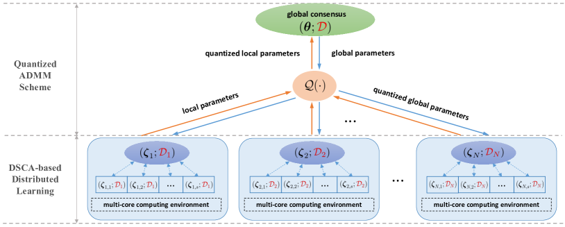
Figure 2: The proposed Sparse LInear Multiple Kernel Learning (SLIM-KL) framework.

IV-A Quantized ADMM

ADMM has emerged as a promising algorithm for developing a principled distributed learning framework [25], enabling multiple agents solve large-scale distributed GPR problems [8]. In this work, we consider a variant of ADMM that incorporates quantization [26, 27], as illustrated in Fig. 2 (Quantized ADMM Scheme). Quantization is a technique widely used in wireless systems to compress information by reducing transmission bits [28, 29]. Mathematically, consider $N\!\in\!\mathbb{N}$ multi-core agents cooperatively learning a global GPR model with the proposed GSMP kernel, the learning problem can be formulated as

$$\min\,\sum_{j=1}^{N}l({\bm{\zeta}}_{j};\mathcal{D}_{j})$$ (15)

$$~{}\operatorname{s.t.}\ {\bm{\zeta}}_{j}-{{\bm{\theta}}}=\bm{0},\ j\in\{1,\ldots,N\},$$

$$\ \qquad{{\bm{\theta}}}\in\Theta,\ {\bm{\zeta}}_{j}\in\Theta,\ j\in\{1,\ldots,N\},$$

where $\mathcal{D}_{j}$ denotes local dataset owned by the $j$-th agent with $|\mathcal{D}_{j}|=n/N$, ${\bm{\zeta}}_{j}$ denotes the local hyper-parameters, and ${{\bm{\theta}}}$ denotes the global hyper-parameters (the weights of GSMP kernel). In this setup, we assume that each agent has the ability to store and perform computations with infinite precision. However, when it comes to transmission, all agents are constrained to sending quantized data that can be received without any error. Let $\Delta>0$ denote the quantization resolution, where smaller $\Delta$ allows more precise transmissions but requires more bits and vice versa. We define the quantization function $\mathcal{Q}:\mathbb{R}\to\Lambda$ that maps a real value to some point in the quantization lattice $\Lambda=\{m\Delta:m\in\mathbb{Z}\}$. Among all the quantizers, we consider the stochastic quantization function [30],

$$\mathcal{Q}(x)=\begin{cases}m\Delta,\enspace\text{with probability}\ m+1-\frac{x}{\Delta},\\ (m+1)\Delta,\enspace\text{with probability}\ \frac{x}{\Delta}-m,\end{cases}$$ (16)

for $x\in[m\Delta,(m+1)\Delta)$. Stochastic quantization introduces noise which can reduce errors in distributed computation compared to deterministic quantization schemes [27]. In Section V, we will establish that quantized ADMM is guaranteed to converge to a stationary point, thanks to the properties of the stochastic quantization used. For ease of notation, we denote $x_{[\mathcal{Q}]}=\mathcal{Q}(x)$ as the quantized value of $x\in\mathbb{R}$.

To solve the optimization problem in Eq. (15), we first formulate the augmented Lagrangian as

$$\quad\mathcal{L}({\bm{\zeta}}_{1},\ldots,{\bm{\zeta}}_{N},{{\bm{\lambda}}}_{1},\ldots,{{\bm{\lambda}}}_{N},{{\bm{\theta}}})$$ (17)

$$\triangleq\sum_{j=1}^{N}\left(l({\bm{\zeta}}_{j};\mathcal{D}_{j})+{{\bm{\lambda}}}_{j}^{\top}({\bm{\zeta}}_{j}-{{\bm{\theta}}})+\frac{\rho_{j}}{2}\|{\bm{\zeta}}_{j}-{{\bm{\theta}}}\|_{2}^{2}\right),$$

where ${{\bm{\lambda}}}_{j}$ is the dual variable and $\rho_{j}$ is a preselected penalty parameter. By imposing a quantization operation on ${{\bm{\theta}}}$ and ${\bm{\zeta}}_{j}$ immediately after the ${{\bm{\theta}}}$-update and ${\bm{\zeta}}_{j}$-update, the sequential update in quantized ADMM for the $(t+1)$-th iteration can be decomposed as

$${{\bm{\theta}}}^{t+1} =\frac{1}{N}\sum_{j=1}^{N}\left(\bm{\zeta}_{j,[\mathcal{Q}]}^{t}+\frac{1}{\rho_{j}}{{\bm{\lambda}}}_{j}^{t}\right),$$ (18a)

$${{\bm{\theta}}}^{t+1}_{[\mathcal{Q}]} =\mathcal{Q}({{\bm{\theta}}}^{t+1}),$$ (18b)

$$\bm{\zeta}_{j}^{t+1} \!=\!\arg\min_{\bm{\zeta}_{j}}\,l\left(\bm{\zeta}_{j};\mathcal{D}_{j}\right)+\left(\bm{\lambda}_{j}^{t}\right)^{\top}\left(\bm{\zeta}_{j}-{{\bm{\theta}}}^{t+1}_{[\mathcal{Q}]}\right)$$

$$\qquad\qquad+\frac{\rho_{j}}{2}\left\|\bm{\zeta}_{j}-{{\bm{\theta}}}^{t+1}_{[\mathcal{Q}]}\right\|_{2}^{2},\ j\in\{1,\ldots,N\},$$ (18c)

$${\bm{\zeta}}^{t+1}_{j,[\mathcal{Q}]} =\mathcal{Q}({\bm{\zeta}}_{j}^{t+1}),$$ (18d)

$$\bm{\lambda}_{j}^{t+1} =\bm{\lambda}_{j}^{t}+\rho_{j}\left(\bm{\zeta}_{j,[\mathcal{Q}]}^{t+1}-{{\bm{\theta}}}^{t+1}_{[\mathcal{Q}]}\right).$$ (18e)

where Eq. (18a) is the quantized ADMM global consensus step, Eq. (18c) is the local update step, and Eq. (18e) is the dual parameters update step. This quantized ADMM scheme allows multiple agents to collaboratively learn the kernel hyper-parameters while preserving data privacy and reducing communication cost. Another useful property of the quantized ADMM is that if one local agent gets stuck at a poor local minimum of the GSMP kernel hyper-parameter, the consensus step may help the agent resume from a more reasonable point in the next iteration.

IV-B DSCA Algorithm

It is worth noting that the local minimization problem formulated in Eq. (18c) is not only non-convex but also non-separable, rendering distributed computation infeasible. Hence, solving it with respect to the entire ${\bm{\zeta}}_{j}$ can be computationally demanding for large $Q$. To alleviate this computational burden, we propose the distributed SCA (DSCA) algorithm to optimize the hyper-parameters in a distributed manner, as depicted in Fig. 2 (DSCA-based Distributed Learning). The key idea is to leverage an $s$-unit computing environment by splitting the hyper-parameters ${\bm{\zeta}}_{j}$ into $s$ blocks and optimize them in parallel across $s$ computing units, $s\!\in\!\mathbb{N}$. By using the fact that the feasible set $\Theta$ in the GSMP kernel admits a Cartesian product structure, i.e., $\Theta=\Theta_{1}\times\Theta_{2}\times\ldots\times\Theta_{s}$ with $\Theta_{i}\subseteq\mathbb{R}^{Q/s}$, we can partition the optimization variable into $s$ blocks, ${\bm{\zeta}}_{j}=[{\bm{\zeta}}_{j,1,}{\bm{\zeta}}_{j,2},\ldots,{\bm{\zeta}}_{j,s}]^{\top}$, and naturally construct the associated surrogate function for $l\left(\bm{\zeta}_{j};\mathcal{D}_{j}\right)$ in Eq. (18c), that is additively separable in the blocks:

$$\tilde{l}({\bm{\zeta}}_{j},{\bm{\zeta}}_{j}^{\eta})=\sum_{i=1}^{s}\tilde{l}_{i}({\bm{\zeta}}_{j,i},{\bm{\zeta}}_{j}^{\eta}).$$ (19)

We make the following assumption on the surrogate function,

Assumption 2.

Each surrogate function $\tilde{l}_{i}({\bm{\zeta}}_{j,i},{\bm{\zeta}}_{j}^{\eta}):\Theta_{i}\times\Theta\mapsto\mathbb{R},i\in\{1,\ldots,s\}$, satisfies the following conditions:

1. $\tilde{l}_{i}({\bm{\zeta}}_{j,i},{\bm{\zeta}}_{j}^{\eta})$ is strongly convex on space $\Theta_{i}$;

2. $\tilde{l}_{i}({\bm{\zeta}}_{j,i},{\bm{\zeta}}_{j}^{\eta})$ is differentiable with

   $$\nabla_{{\bm{\zeta}}_{j,i}}\tilde{l}_{i}({\bm{\zeta}}_{j,i},{\bm{\zeta}}_{j}^{\eta})=\nabla_{{\bm{\zeta}}_{j,i}}l({\bm{\zeta}}_{j})\big{|}_{{\bm{\zeta}}_{j}={\bm{\zeta}}_{j}^{\eta}}.$$ (20)

To fulfill the two conditions in Assumption 2, we can use a similar strategy as the vanilla SCA, and construct $\tilde{l}_{i}({\bm{\zeta}}_{j,i},{\bm{\zeta}}_{j}^{\eta})$ in Eq. (19) as

$$\tilde{l}_{i}({\bm{\zeta}}_{j,i},{\bm{\zeta}}_{j}^{\eta})\!=\!g({\bm{\zeta}}_{j,i},{\bm{\zeta}}_{j,-i}^{\eta})-h({\bm{\zeta}}_{j}^{\eta})-\nabla_{{\bm{\zeta}}_{j,i}}h({\bm{\zeta}}_{j}^{\eta})^{\top}({\bm{\zeta}}_{j,i}-{\bm{\zeta}}_{j,i}^{\eta}),$$ (21)

where

$$\nabla_{{\bm{\zeta}}_{j,i}}h({\bm{\zeta}}_{j}^{\eta})=\left.\begin{bmatrix}-\operatorname{Tr}\left(\bm{C}^{-1}({\bm{\zeta}}_{j})\frac{\partial\bm{C}({\bm{\zeta}}_{j})}{\partial\zeta_{j,1+(i-1)Q/s}}\right)\\ -\operatorname{Tr}\left(\bm{C}^{-1}({\bm{\zeta}}_{j})\frac{\partial\bm{C}({\bm{\zeta}}_{j})}{\partial\zeta_{j,2+(i-1)Q/s}}\right)\\ \vdots\\ -\operatorname{Tr}\left(\bm{C}^{-1}({\bm{\zeta}}_{j})\frac{\partial\bm{C}({\bm{\zeta}}_{j})}{\partial\zeta_{j,iQ/s}}\right)\end{bmatrix}\right|_{{\bm{\zeta}}_{j}={\bm{\zeta}}_{j}^{\eta}}$$

and ${\bm{\zeta}}_{j,-i}^{\eta}=\left[{\bm{\zeta}}_{j,1}^{\eta},\ldots,{\bm{\zeta}}_{j,i-1}^{\eta},{\bm{\zeta}}_{j,i+1}^{\eta},\ldots,{\bm{\zeta}}_{j,s}^{\eta}\right]^{\top}$. Note that $\tilde{l}({\bm{\zeta}}_{j},{\bm{\zeta}}_{j}^{\eta})$ in Eq. (19) also satisfies the two conditions in Assumption 1. Thus, DSCA first solves the following convex optimization problem in parallel for all $i\in\{1,\ldots,s\}$:

$${{\bm{\zeta}}}_{j,i}^{\eta+1}=\arg\min_{{\bm{\zeta}}_{j,i}}\,\ell({\bm{\zeta}}_{j,i},{\bm{\zeta}}_{j}^{\eta})$$ (22)

where $\ell({\bm{\zeta}}_{j,i},{\bm{\zeta}}_{j}^{\eta})\!\triangleq\!\tilde{l}_{i}({\bm{\zeta}}_{j,i},{\bm{\zeta}}_{j}^{\eta})\!+\!\left(\bm{\lambda}_{j,i}^{t}\right)^{\top}\!\!\left({\bm{\zeta}}_{j,i}\!-\!{{\bm{\theta}}}_{i}^{t+1}\right)\!+\!\frac{\rho_{j}}{2}\left\|{\bm{\zeta}}_{j,i}-{{\bm{\theta}}}_{i}^{t+1}\right\|_{2}^{2}$. However, it has been observed that directly using CVX [31, 32], a package designed for constructing and solving convex programs, to solve Eq. (22) is computationally demanding. Since the term $\tilde{l}_{i}({\bm{\zeta}}_{j,i},{\bm{\zeta}}_{j}^{\eta})$ in Eq. (22) contains a matrix fractional component, we can reformulate the problem into a conic form, with the introducing auxiliary variables $\bm{z},\bm{w},v$:

$$\min_{{\bm{\zeta}}_{j,i},\bm{z},\bm{w},v}\,(\bm{1}^{\top}\bm{z})+\left({{\bm{\lambda}}}_{j,i}^{t}-\nabla_{{\bm{\zeta}}_{j,i}}h({\bm{\zeta}}_{j}^{\eta})\right)^{\top}{\bm{\zeta}}_{j,i}+\frac{\rho_{j}}{2}v$$

$$\text{s.t.}\,\enspace\left\|\begin{bmatrix}2\bm{w}_{0},\\ z_{0}-1\end{bmatrix}\right\|_{2}\leq z_{0}+1,$$

$$\hskip 17.86797pt\left\|\begin{bmatrix}2\bm{w}_{k},\\ z_{k}-{\bm{\zeta}}_{j,k+(i-1)Q/s}\end{bmatrix}\right\|_{2}\leq z_{k}+{\bm{\zeta}}_{j,k+(i-1)Q/s},$$

$$\hskip 131.31903ptk\in\{1,2,\ldots,Q/s\},$$

$$\hskip 19.37494pt\bm{y}=\sum_{k=1}^{Q/s}\bm{L}_{k+(i-1)Q/s}\bm{w}_{k}$$

$$\hskip 21.52771pt+\left(\sum_{n\neq i}\sum_{k=1}^{Q/s}{\bm{\zeta}}_{j,k+(n-1)Q/s}^{\eta}\bm{K}_{k+(n-1)Q/s}+\sigma_{e}^{2}\bm{I}_{n}\right)^{\frac{1}{2}}\!\bm{w}_{0},$$

$$\hskip 20.45132pt2v\frac{1}{2}\geq\sum_{k=1}^{Q/s}\left({\bm{\zeta}}_{j,k+(i-1)Q/s}-{{\bm{\theta}}}_{k+(i-1)Q/s}^{t+1}\right)^{2},$$

$$\hskip 20.45132pt{\bm{\zeta}}_{j,i}\geq\bm{0},\enspace\bm{z}\geq\bm{0}.$$ (23)

where $v\geq 0$. We provide the detailed steps for this reformulation in Appendix C. The problem presented in Eq. (IV-B) is now in conic form and can be solved more efficiently using MOSEK [19, 10]. After the local agents have optimized their local hyper-parameters using DSCA in the $t$-th iteration, the ADMM consensus step formulated in Eq. (18a) is conducted to reach a global consensus. At this point, we have introduced the SLIM-KL framework. The pseudocode for implementing SLIM-KL is summarized in Algorithm 1.

Remark 1.

By leveraging $N$ local agents and $s$ computing units, the overall computational complexity of SLIM-KL at each iteration is reduced from $\mathcal{O}(Qn^{3})$ to $\mathcal{O}(\frac{Qn^{3}}{sN^{3}})$. That is, as the number of agents $N$ and computing units $s$ increase, the computational burden of optimizing the hyper-pameters can be significantly reduced especially when dealing with large values of grid points $Q$ and training size $n$.

Remark 2.

The design of SLIM-KL matches perfectly with the sparse nature of the proposed GSMP kernel, see Theorem 3. Many weights/hyper-parameters of the sub-kernels in the GSMP kernel are inherently zero or near-zero valued, so quantization can enhance this sparsity by rounding even more of these weights to zero. This enhanced sparsity could aid convergence and guide the algorithm toward a favorable local minimum, as noted in [26].

1 Initialization: $t=0$, $\{\rho_{j},\bm{\zeta}_{j}^{0},\bm{\lambda}_{j}^{0}\}_{j=1}^{N}$, $N$ local datasets $\{\mathcal{D}_{j}\}_{j=1}^{N}$ in $N$ local computing agents, quantization function $\mathcal{Q}(\cdot)$;

2 while Iteration stopping criteria are not satisfied do

3       Obtain the global hyper-parameters $\bm{\theta}^{t+1}$ by Eq. (18a);

4      Apply quantization on the global hyper-parameters using Eq. (18b) and obtain ${{\bm{\theta}}}^{t+1}_{[\mathcal{Q}]}$;

5      for $j\in[1,N]$ do

6             Obtain the local hyper-parameters $\bm{\zeta}_{j}^{t+1}$ by utilizing DSCA to solve Eq. (IV-B) in parallel using $s$ units;

7            Apply quantization on the local hyper-parameters using Eq. (18d) and obtain ${\bm{\zeta}}^{t+1}_{j,[\mathcal{Q}]}$;

8       end for

9      

10      Obtain the dual variables by Eq. (18e);

11 end while

return $\bm{\theta}^{t}$

Algorithm 1 SLIM-KL for LMK learning

V Analysis

In this section, we present the theoretical analysis of the SLIM-KL framework proposed in Section IV.

First, we show that the DSCA algorithm solving the local minimization problem within quantized ADMM is guaranteed to be converged, which is succinctly summarized as follows.

Theorem 4.

By employing DSCA, the objective of the local minimization problem, see Eq. (18c), is non-increasing, and the sequence of feasible points $\{{\bm{\zeta}}_{j}^{\eta}\}_{\eta\in\mathbb{N}}$ satisfies,

$$\lim_{\eta\to\infty}\|{\bm{\zeta}}_{j}^{\eta+1}-{\bm{\zeta}}_{j}^{\eta}\|=0.$$ (24)

Proof.

The proof can be found in Appendix D. ∎

Theorem 4 suggests that within the iteration of quantized ADMM, the local minimization problem is solved exactly [33]. Building upon the result from Theorem 4, next, we can show that the quantized ADMM-based SLIM-KL framework is guaranteed to reach a stationary point in a mean sense, as summarized in the following theorem.

Theorem 5.

The SLIM-KL framework ensures that: Under the stochastic quantization scheme, the sequence $\{{\bm{\zeta}}_{j}^{t}\}_{j=1}^{N}$ converges to ${{\bm{\theta}}}^{t}$ in the mean sense as $t\to\infty$, with the variance of ${\bm{\zeta}}_{j}^{t}$ stabilizing at a finite value which depends on the quantization resolution $\Delta$.

Proof.

We first refer to the following lemma,

Lemma 1.

With stochastic quantization, each $x\in\mathbb{R}$ can be unbiasedly estimated as

$$\mathbb{E}[\mathcal{Q}(x)]=x,$$ (25)

and the associated quantization error is bounded by

$$\mathbb{E}\left[(x-\mathcal{Q}(x))^{2}\right]\leq\frac{\Delta^{2}}{4}.$$ (26)

Proof.

The proof can be found in Appendix E. ∎

It follows that, by taking expectation on both sides of Eq. (18a) and Eq. (18e) we can get,

$$\mathbb{E}\left[{{\bm{\theta}}}^{t+1}\right] =\frac{1}{N}\sum_{j=1}^{N}\left(\mathbb{E}\left[\bm{\zeta}_{j,[\mathcal{Q}]}^{t}\right]+\frac{1}{\rho_{j}}\mathbb{E}\left[{{\bm{\lambda}}}_{j}^{t}\right]\right),$$ (27a)

$$\mathbb{E}\left[\bm{\lambda}_{j}^{t+1}\right] =\mathbb{E}\left[\bm{\lambda}_{j}^{t}\right]+\rho_{j}\left(\mathbb{E}\left[\bm{\zeta}_{j,[\mathcal{Q}]}^{t+1}\right]-\mathbb{E}\left[{{\bm{\theta}}}^{t+1}_{[\mathcal{Q}]}\right]\right).$$ (27b)

Note that Lemma 1 implies that $\mathbb{E}[\bm{\zeta}_{j,[\mathcal{Q}]}^{t+1}]={\bm{\zeta}}_{j}^{t+1}$ and $\mathbb{E}[{{\bm{\theta}}}^{t+1}_{[\mathcal{Q}]}]={{\bm{\theta}}}^{t+1}$. Since $\mathbb{E}[{{\bm{\lambda}}}_{j}^{0}]={{\bm{\lambda}}}_{j}^{0}$, it is easy to see that Eq. (27a) and Eq. (27b) takes exactly the same iterations in the mean sense as the consensus ADMM, i.e., ADMM without quantization scheme. Therefore, the convergence in mean of $\{{\bm{\zeta}}_{j}^{t}\}_{j=1}^{N}$ to ${{\bm{\theta}}}^{t}$ is guaranteed due to the convergence of consensus ADMM established in [25, 34, 27]. Moreover, Lemma 1 also indicates the bounded variance of quantization error, so the variance of ${\bm{\zeta}}_{j}^{t}$ stabilizes to a finite value that depends on the quantization resolution $\Delta$ [26]. Thus, we have established the convergence in mean of $\{{\bm{\zeta}}_{j}^{t}\}_{j=1}^{N}$ to ${{\bm{\theta}}}^{t}$ with a stabilized variance as $t\to\infty$, completing the proof for Theorem 5. ∎

VI Experiments

In this section, we provide experimental validation for the kernel formulation and learning framework proposed in Sections III and IV. The efficiency and approximation capability of the proposed GSMP kernel are demonstrated in Section VI-A, followed by a comparative analysis between our method and some competing approaches in Section VI-B. Lastly, Sections VI-C and VI-D highlight the scalability and communication efficiency of our learning framework. Our implementation code is accessible at https://github.com/richardcsuwandi/SLIM-KL.

VI-A Approximation Capability of GSMP Kernel

This subsection demonstrates the modeling property of the GSMP kernel. To empirically substantiate our claims presented in Section III, we synthetically generate a dataset consisting of 500 samples from a GP with the SM kernel. The GP inputs corresponding to the dataset are uniformly distributed within the domain $[0,10]^{2}$. Subsequently, we utilize 480 data for the training of GPs employing the GSM kernel and the GSMP kernel, respectively. The remaining 20 data points are reserved for testing. For the comparison, we set $Q=50$ and sample the grid points from only the positive quadrant, that is, $\mu_{q}^{(p)}$ are uniformly sampled from $[0,3]$ and the variance variables $v_{q}^{(p)}$ are set to $0.01$. The learning results of GPs employing the GSM and GSMP kernels are demonstrated by employing diverse hyper-parameter configurations for the underlying SM kernel. These configurations correspond to different datasets, as outlined below.

• Configuration 1: The SM kernel has an underlying four-mode Gaussian mixture spectral density, $S(\bm{\omega})=\sum_{i=1}^{4}\alpha_{i}\mathcal{N}(\bm{\mu}_{i},\bm{V}_{i})$, where $\alpha_{1}=\ldots=\alpha_{4}=5$, $\bm{\mu}_{1}=[-2,-2]^{\top}$, $\bm{\mu}_{2}=[-2,2]^{\top}$, $\bm{\mu}_{3}=[2,-2]^{\top},\bm{\mu}_{4}=[2,2]^{\top}$, and $\bm{V}_{1}=\ldots=\bm{V}_{4}=0.1\bm{I}$.

• Configuration 2: The SM kernel has an underlying four-mode Gaussian mixture spectral density, $S(\bm{\omega})=\sum_{i=1}^{4}\alpha_{i}\mathcal{N}(\bm{\mu}_{i},\bm{V}_{i})$, where $\alpha_{1}=\ldots=\alpha_{4}=5$, $\bm{\mu}_{1}=[-2,-2]^{\top}$, $\bm{\mu}_{2}=[-3,3]^{\top}$, $\bm{\mu}_{3}=[3,-3]^{\top},\bm{\mu}_{4}=[2,2]^{\top}$, and $\bm{V}_{1}=\ldots=\bm{V}_{4}=0.1\bm{I}$.

• Configuration 3: The SM kernel has an underlying two-mode Gaussian mixture spectral density, $S(\bm{\omega})=\sum_{i=1}^{2}\alpha_{i}\mathcal{N}(\bm{\mu}_{i},\bm{V}_{i})$, where $\alpha_{1}=\alpha_{2}=5$, $\bm{\mu}_{1}=[-2,-2]^{\top}$, $\bm{\mu}_{2}=[2,2]^{\top}$, and $\bm{V}_{1}=\bm{V}_{2}=0.1\bm{I}$.

• Configuration 4: The SM kernel has an underlying four-mode Gaussian mixture spectral density, $S(\bm{\omega})=\sum_{i=1}^{4}\alpha_{i}\mathcal{N}(\bm{\mu}_{i},\bm{V}_{i})$, where $\alpha_{1}=\alpha_{4}=15$, $\alpha_{2}=\alpha_{3}=5$ $\bm{\mu}_{1}=[-2,-2]^{\top}$, $\bm{\mu}_{2}=[-3,3]^{\top}$, $\bm{\mu}_{3}=[3,-3]^{\top},\bm{\mu}_{4}=[2,2]^{\top}$, and $\bm{V}_{1}=\ldots=\bm{V}_{4}=0.1\bm{I}$.

• Configuration 5: The SM kernel has an underlying six-mode Gaussian mixture spectral density, $S(\bm{\omega})=\sum_{i=1}^{6}\alpha_{i}\mathcal{N}(\bm{\mu}_{i},\bm{V}_{i})$, where $\alpha_{1}=\alpha_{6}=10,\alpha_{2}=\alpha_{5}=10,\alpha_{3}=\alpha_{4}=5$, $\bm{\mu}_{1}=[0.1,0.1]^{\top}$, $\bm{\mu}_{2}=[1,1]^{\top}$, $\bm{\mu}_{3}=[1.5,1.5]^{\top},\bm{\mu}_{4}=[-1.5,-1.5]^{\top}$, $\bm{\mu}_{5}=[-1,-1]^{\top}$, $\bm{\mu}_{6}=[-0.1,-0.1]^{\top}$, and $\bm{V}_{1}=\ldots=\bm{V}_{6}=0.05\bm{I}$.

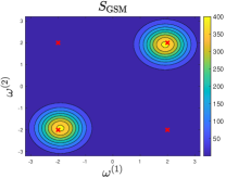
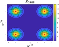
(a) Configuration 1

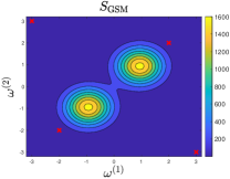
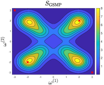
(b) Configuration 2

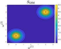
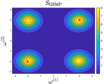
(c) Configuration 3

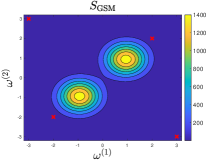
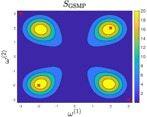
(d) Configuration 4

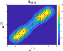
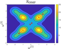
(e) Configuration 5

Figure 3: The learned spectral density of multi-dimensional GSM kernel (left) versus the learned spectral density of GSMP kernel (right). The cross symbols represent the modes of the ground truth.

The spectral density results of the learned kernels are depicted in Fig. 3, and the GP prediction results are presented in Table I. From the results of configurations 1, 2, and 4, we can observe that when the density modes of the underlying kernel lie in the main diagonal, as illustrated in the corresponding subfigures of Fig. 3, the GSM kernel struggles to represent the density in this diagonal accurately. This arises because the grid points fixed by the GSM only support the density on the negative diagonal but fall short of accommodating the density on the main diagonal. In contrast, the GSMP kernel contains additional $2Q$ Gaussian densities, enabling it to capture the main diagonal’s density effectively. This superior fitting of the underlying density translates into GSMP’s enhanced prediction performance, as corroborated by the results shown in Table I. If one wants to compensate for the performance deficiencies of the GSM kernel function, it requires fixing additional $Q$ grid points, totaling $2Q$ grid points, for the GSM. Conversely, the GSMP kernel achieves comparable performance while only requiring $Q$ grid points.

On the other hand, the results of configurations 3 and 5 reveal that when the density pattern of the underlying kernel exclusively aligns with the sub-diagonal, as depicted in the corresponding subfigure of Fig. 3, the GSM kernel adeptly approximates this diagonal density. In comparison to GSM, the GSMP kernel not only encompasses the underlying sub-diagonal density but also introduces additional density on the main diagonal. However, the GP prediction performance using the GSMP kernel, as showcased in Table I, demonstrates a marginal difference from the performance achieved with the GSM kernel. This underscores that the supplementary density incorporated within the GSMP kernel has a relatively subdued impact on GP prediction results.

The above empirical findings highlight that the GSMP kernel not only effectively approximates the underlying kernel, ensuring commendable GP prediction performance, but notably diminishes the number of fixed grid points/sub-kernels. This reduction significantly mitigates both model and computational complexities, rendering it suitable for handling higher-dimensional data.

TABLE I: Prediction mean squared error (MSE) of the GP with GSMP kernel versus the GP with GSM kernel [12]

. Configuration 1 2 3 4 5 GSM 0.0172 0.5564 0.0046 0.9431 7.2646E-03 GSMP 0.0101 0.1732 0.0063 0.3769 8.3232E-03

TABLE II: Performance comparison between the proposed GSMGP with SLIM-KL ($s=4,N=2,\Delta=0.01$) and their competitors in terms of the prediction MSE. The lowest MSE value is highlighted in bold. The percentage in the brackets indicates the sparsity level of the solution. The lower the value, the sparser the solution.

Dataset	GSMPGP	GSMGP	SMGP	SEGP	LSTM	Informer
ECG	1.2E-02  (0.8%)	1.2E-02  (0.8%)	1.9E-02  (100%)	1.6E-01	1.6E-01	5.4E-02
CO2	3.7E-01  (0.6%)	6.2E-01  (1.0%)	7.4E-01  (100%)	1.5E+03	2.9E+02	8.4E+01
Unemployment	2.0E+03  (2.8%)	2.2E+03  (4.6%)	7.7E+03  (100%)	5.6E+05	1.7E+05	3.8E+03
ALE	2.5E-02  (0.25%)	1.9E+00  (0.5%)	3.7E-01  (100%)	3.7E-02	3.4E-02	1.8E-01
CCCP	1.6E+01  (0.25%)	1.9E+02  (0.25%)	2.1E+05  (100%)	1.7E+01	2.8E+02	1.4E+05
Toxicity	1.4E+00  (1.13%)	2.7E+02  (1.13%)	5.3E+00  (100%)	1.4E+00	1.7E+00	2.9E+00
Concrete	5.9E+01  (0.13%)	5.6E+02  (0.25%)	1.7E+03  (100%)	1.3E+02	1.4E+02	2.0E+02
Wine	4.6E-01  (0.09%)	7.4E+03  (0.09%)	3.1E+01  (100%)	4.4E+00	4.7E-01	1.6E+00
Water	1.6E-04  (1.27%)	1.7E-04  (1.0 %)	5.5E-03  (100%)	1.6E-04	4.2E-04	9.2E-02

VI-B Prediction Performance

This subsection presents the prediction performance of the proposed GSMP kernel-based GP (GSMPGP) trained using the SLIM-KL framework on nine real-world datasets. The dimensionality of these datasets varies from $1$ to $11$, details can be found in Appendix G. The setup for training the GSMPGP is listed as follows. The number of mixture components $Q$ is set to 500 for the one-dimensional case and $100\times P$ for the multi-dimensional case. The mean variables $\mu_{q}^{(p)}$ are uniformly sampled from the frequency range mentioned in Appendix F and the variance variables $v_{q}^{(p)}$ are fixed to a small constant, $0.001$. The weights $\bm{\theta}$ and the dual variables $\{\bm{\lambda}_{j}\}_{j=1}^{N}$ are initialized to zeros. The penalty parameter $\{\rho_{j}\}_{j=1}^{N}$ is initialized to $10^{-10}$ and adaptively updated using the residual balancing strategy [35]. The noise variance parameter $\sigma_{e}^{2}$ is estimated using a cross-validation filter type method [36].

For comparison, we consider five other models, the original GSM kernel-based GP (GSMGP) [12], an SM kernel-based GP (SMGP) [9], a squared-exponential kernel-based GP (SEGP) [2], a long short-term memory (LSTM) recurrent neural network [37], and a very recent Transformer-based time series prediction model, Informer [38]. The SMGP and SEGP model hyper-parameters are optimized using a gradient-descent based approach with the default parameter settings suggested in https://people.orie.cornell.edu/andrew/code. The GSM and SM kernel use the same number of kernel components as the GSMP kernel ($Q=500$ or $Q=100\times P$) for a fair comparison. The LSTM model has a standard architecture with 3 hidden layers, each with 100 hidden units while the Informer model follows the default configuration as specified in https://github.com/zhouhaoyi/Informer2020/tree/main.

Table II shows the prediction performance of various models as measured by the mean-squared-error (MSE). These results demonstrate that the proposed GSMGP consistently outperform their competitors in prediction MSE across all datasets. Notably, the GSMGP kernel outperforms the original GSM kernel’s, particularly in multi-dimensional datasets, aligning with our findings in Section VI-A. While classical models like LSTM, and more recent models like Informer, require long time series data to learn the underlying patterns effectively, our GSMPGP model excels by building the correlations between series data and minimizing the negative marginal log-likelihood to optimize the kernel hyper-parameters. Furthermore, our GSMPGP model surpasses both the SMGP and other GP models employing basic kernels, such as SEGP, demonstrating our model’s superior performance relative to its competitors.

The improved prediction performance not only comes from the flexible model capacity of GSMPGP, but also benefits from the inherent sparsity in the solutions it generates. The sparsity level of the solutions, calculated as the ratio of nonzero elements to the total number of elements, is reported in Table II. We note that both GSMPGP and GSMGP obtain sparse solutions, in comparison to SMGP. By pinpointing only the significant sub-kernels, GSMPGP and GSMGP avoid over-parameterization, yielding better generalization capaibility and lower prediction MSE.

VI-C Scalability

This subsection aims to investigate the scalability of SLIM-KL through experiments with varying numbers of computing units and agents. We first consider varying $s\in\{1,4,10,50,100\}$, and evaluate the performance based on the prediction MSE and computation time (CT). Results in Table III show that the prediction MSE does not always worsens as $s$ increases. In fact, for several datasets, an improved MSE can be achieved when using more than one computing unit. Moreover, Fig. 4 highlights the advantage of using multiple computing units in reducing the overall CT, supporting the result given in Remark 1.

TABLE III: Performance of SLIM-KL ($N=2,\Delta=0.01$) with varying number of computing units $s$, in terms of the prediction MSE. The lowest MSE value for each dataset is highlighted in bold.

Dataset	$s=1$	$s=4$	$s=10$	$s=50$	$s=100$
ECG	1.2E-02	1.2E-02	1.2E-02	1.5E-02	1.5E-02
CO2	4.9E-01	3.7E-01	6.2E-01	1.1E+00	6.6E-01
Unemployment	2.3E+03	2.0E+03	2.2E+03	2.2E+03	3.3E+03
ALE	2.5E-02	2.5E-02	2.5E-02	2.5E-02	2.5E-02
CCCP	1.6E+01	1.6E+01	1.6E+01	1.6E+01	1.6E+01
Toxicity	1.4E+00	1.4E+00	1.4E+00	1.4E+00	1.4E+00
Concrete	5.9E+01	5.9E+01	5.9E+01	5.9E+01	5.9E+01
Water	1.6E-04	1.6E-04	1.6E-04	1.6E-04	1.6E-04
Wine	4.6E-01	4.6E-01	4.6E-01	4.6E-01	4.6E-01

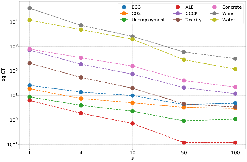
Figure 4: Total computation time (in log-scale) for one computing unit, with respect to different values of $s$.

We also test the effect of varying the number of local agents on the prediction performance of SLIM-KL. In particular, we set $N\in\{2,4,8,10\}$ and compare them with the centralized case which serves as the baseline. The results in Table IV illustrate that SLIM-KL performs better on nearly all datasets when using multiple local agents compared to the centralized case. However, when $N$ is set to be relatively large compared to the size of the training set, the prediction performance degrades as each local agent has fewer data available for training, as evident, e.g., in the Unemployment dataset. Hence, there is a trade-off between leveraging more distributed agents and ensuring each agent has sufficient data for training.

TABLE IV: Performance of SLIM-KL ($s=4,\Delta=0.01$) with varying number of local agents $N$, in terms of the prediction MSE. The lowest MSE value for each dataset is highlighted in bold.

Dataset	Centralized	$N=2$	$N=4$	$N=8$	$N=10$
ECG	1.2E-02	1.2E-02	1.3E-02	1.4E-02	2.2E-02
CO2	4.5E-01	3.7E-01	5.3E-01	8.0E-01	5.7E-01
Unemployment	2.3E+03	2.0E+03	4.9E+03	8.2E+03	9.1E+03
ALE	2.5E-02	2.5E-02	2.5E-02	2.5E-02	2.5E-02
CCCP	1.6E+01	1.6E+01	1.6E+01	1.6E+01	1.6E+01
Toxicity	1.4E+00	1.4E+00	1.8E+00	1.7E+00	1.8E+00
Concrete	8.3E+01	5.9E+01	8.4E+01	8.4E+01	8.5E+01
Water	1.6E-04	1.6E-04	1.6E-04	1.6E-04	1.7E-04
Wine	4.6E-01	4.6E-01	4.7E-01	4.9E-01	5.3E-01

To further evaluate the scalability of SLIM-KL, we test its performance on a large dataset. Specifically, we consider the CCCP dataset and increase the training set size $|\mathcal{D}|$ to 9500 and the test set size $|\mathcal{D}_{*}|$ to 68. We set $N=10$ and $s=4$ while keeping the other experimental setup unchanged. Remarkably, we observed that SLIM-KL continues to perform well even with a dataset nearly ten times larger. The prediction MSE remains low at 1.6E+01, highlighting the algorithm’s ability to handle big data.

VI-D Effect of Quantization

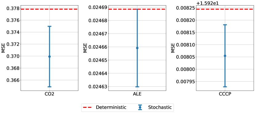
Figure 5: Performance comparison of SLIM-KL under stochastic quantization versus deterministic quantization, with $\Delta=0.01$. The blue dots with vertical error bars indicate the mean MSE plus-minus two standard deviations when using the stochastic quantization, while the red dashed lines represent the MSE when using the deterministic quantization.

This subsection studies the effect of quantization on the performance of SLIM-KL through ablation experiments. We compare two different choices of quantization scheme: stochastic quantization and deterministic quantization. Due to the random nature of the stochastic quantization, we repeat each experiment 5 times and report the mean MSE with corresponding error bars. Fig. 5 reveals that the stochastic quantization scheme achieves a consistently lower MSE than deterministic quantization, despite its variability. The error bars, denoting plus-minus two standard deviations, suggest that while the MSE for stochastic quantization varies, it does so within a bounded variance, indicating a reliable performance with potential benefits from its inherent randomness.

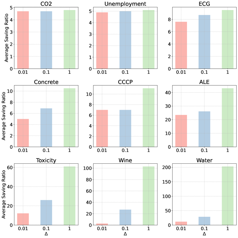
Figure 6: Average saving ratio in transmitting the local hyper-parameters when using quantization versus without quantization, with respect to different quantization resolution $\Delta$.

We further study the performance of SLIM-KL under different quantization resolution $\Delta\in\{0.01$, $0.1,1\}$ and compare them with the case without quantization. To evaluate the performance, we empirically compute the prediction MSE and the number of bits required to transmit the local hyper-parameters. Assuming double precision, the size of the communication overhead for transmitting a normal vector $\bm{x}\in\mathbb{R}^{d}$ is $B=64d$ bits, while for the quantized vector $\mathcal{Q}(\bm{x})$ it is $B_{\mathcal{Q}}=d\log_{2}\left((x_{\text{max}}-x_{\text{min}})/\Delta+1\right)$ bits, where $x_{\text{max}}$ and $x_{\text{min}}$ denote the largest and smallest entry of $\bm{x}$, respectively. Thus, the saving ratio in transmission bits when using quantized can be computed as,

$$\frac{B}{B_{\mathcal{Q}}}=\frac{64}{\log_{2}((x_{\text{max}}-x_{\text{min}})/\Delta+1)}.$$ (28)

Results in Table V demonstrate that quantization does not necessarily degrade prediction performance. In fact, on the CO2 dataset, setting $\Delta=1$ yields the lowest prediction MSE while saving $4.8\times$ fewer bits on average, as depicted in Fig. 6. This improved performance corroborates the design of SLIM-KL, where the enhanced sparsity can be beneficial in guiding the algorithm towards a more favorable optimum, as elaborated in Remark 2. Overall, quantization demonstrate remarkable communication cost savings of at most, over 200 times in the Water dataset, while maintaining promising prediction performance.

TABLE V: Performance of SLIM-KL ($s=4,N=2$) with and without quantization in terms of the prediction MSE. The lowest MSE value is highlighted in bold.

Dataset	Without Quantization	With Quantization
		$\Delta=0.01$	$\Delta=0.1$	$\Delta=1$
ECG	1.2E-02	1.2E-02	2.7E-02	1.6E-01
CO2	3.7E-01	3.7E-01	6.5E-01	2.7E-01
Unemployment	2.0E+03	2.0E+03	2.0E+03	2.0E+03
ALE	2.5E-02	2.5E-02	2.5E-02	2.5E-02
CCCP	1.6E+01	1.6E+01	1.6E+01	1.6E+01
Toxicity	1.4E+00	1.4E+00	1.4E+00	1.4E+00
Concrete	5.9E+01	5.9E+01	5.9E+01	5.9E+01
Water	1.6E-04	1.6E-04	1.6E-04	4.4E-01
Wine	4.6E-01	4.6E-01	4.6E-01	4.6E-01

VII Conclusion

In this paper, we proposed a novel GP kernel and a generic sparsity-aware distributed learning framework for linear multiple kernel learning. Our experiments verified that the GSMP kernel, requiring only a modest number of hyper-parameters, retains a commendable approximation capability for multi-dimensional data. Moreover, the GSMGP with SLIM-KL exhibits superior prediction performance over its competitors across diverse datasets. The scalability test further revealed that SLIM-KL maintains and improves prediction performance with an increased number of computing units and agents, demonstrating the framework’s effectiveness for distributed computing environments. Additionally, the incorporation of stochastic quantization schemes further enhanced the practicality of SLIM-KL by significantly reducing communication overhead while preserving performance.

Appendix A Spectral Density of GSMP Kernel

We prove Theorem 2. By taking the Fourier transform of the GSMP kernel given in Eq. (11), its spectral density can be obtained as,

$$S_{\mathrm{GSMP}}(\bm{\omega})$$ (29)

$$=\int_{\mathbb{R}^{P}}k(\bm{\tau})\exp\left\{-j2\pi\bm{\tau}^{\top}\bm{\omega}\right\}d\bm{\tau}$$

$$=\int_{\mathbb{R}^{P}}\sum_{q=1}^{Q}\theta_{q}\prod_{p=1}^{P}k_{q}\left(\tau^{(p)}\right)\exp\left\{-j2\pi\bm{\tau}^{\top}\bm{\omega}\right\}d\bm{\tau}$$

$$=\sum_{q=1}^{Q}\theta_{q}\prod_{p=1}^{P}\underbrace{\left[\int_{\mathbb{R}}k_{q}\left(\tau^{(p)}\right)\exp\left\{-j2\pi\tau^{(p)}\omega^{(p)}\right\}d\tau^{(p)}\right]}_{\text{Fourier transform of $k_{q}\left(\tau^{(p)}\right):$}\ \mathcal{F}\left[k_{q}\left(\tau^{(p)}\right)\right]}$$

Subsituting the definition of $k_{q}\left(\tau^{(p)}\right)$ yields,

$$\mathcal{F}\left[k_{q}\left(\tau^{(p)}\right)\right]$$ (30)

$$=\mathcal{F}\left[\exp\left\{-2\pi^{2}{\tau^{(p)^{2}}}v_{q}^{{(p)}}\right\}\cos\left(2\pi\tau^{(p)}\mu_{q}^{(p)}\right)\right]$$

$$=\mathcal{F}\left[\exp\left\{-2\pi^{2}{\tau^{(p)^{2}}}v_{q}^{{(p)}}\right\}\right]*\mathcal{F}\left[\cos\left(2\pi\tau^{(p)}\mu_{q}^{(p)}\right)\right]$$

$$=\frac{1}{\sqrt{{2\pi v_{q}^{(p)}}}}\exp\left\{\!-\frac{\omega^{{(p)}^{2}}}{2v_{q}^{(p)}}\!\right\}*\frac{1}{2}\big{(}\delta(\omega^{(p)}\!-\!\mu_{q}^{(p)})$$

$$\hskip 8.61108pt+\,\delta(\omega^{(p)}+\mu_{q}^{(p)})\big{)}$$

$$=\frac{1}{2}\left[\frac{1}{\sqrt{{2\pi v_{q}^{(p)}}}}\exp\left\{-\frac{\left(\omega^{(p)}-\mu_{q}^{(p)}\right)^{2}}{2v_{q}^{(p)}}\right\}\right.$$

$$\hskip 19.37494pt\left.+\frac{1}{\sqrt{{2\pi v_{q}^{(p)}}}}\exp\left\{-\frac{\left(\omega^{(p)}+\mu_{q}^{(p)}\right)^{2}}{2v_{q}^{(p)}}\right\}\right]$$

$$=\frac{1}{2}\left[\mathcal{N}\left(\omega^{(p)}\mid\mu_{q}^{(p)},v_{q}^{(p)}\right)+\mathcal{N}\left(\omega^{(p)}\mid-\mu_{q}^{(p)},v_{q}^{(p)}\right)\right]$$

Therefore, the spectral density of the GSMP kernel is given by,

$$S_{\mathrm{GSMP}}(\bm{\omega})=\sum_{q=1}^{Q}\theta_{q}\prod_{p=1}^{P}\mathcal{F}\left[k_{q}\left(\tau^{(p)}\right)\right]$$ (31)

$$=\frac{1}{2^{P}}\sum_{q=1}^{Q}\theta_{q}\prod_{p=1}^{P}\left[\mathcal{N}\!\left(\omega^{(p)}\mid\mu_{q}^{(p)},v_{q}^{(p)}\!\right)\!+\!\mathcal{N}\!\left(\omega^{(p)}\mid\!-\!\mu_{q}^{(p)},v_{q}^{(p)}\!\right)\right]$$

which is a Gaussian mixture.

Appendix B Proof of Theorem 3

Proof.

The proof is an extension of [39, Theorem 2]. We first state the following lemma that is necessary for the final result.

Lemma 2 (Section IV.A [39]).

The term $\bm{y}^{\top}\bm{C}^{-1}(\bm{\theta})\bm{y}$ equals a constant $C$ over all ${{\bm{\theta}}}$ satisfying the $n$ linear constraints $\bm{A}\bm{\theta}=\bm{b}$ where,

$$\bm{A}\triangleq[\bm{v}_{1},\bm{v}_{2},\ldots,\bm{v}_{Q}],\ \ \bm{b}\triangleq\bm{y}-\sigma_{e}^{2}\bm{u},$$ (32)

with $\bm{v}_{q}\triangleq\bm{K}_{q}\bm{u}$ and $\bm{u}$ is any fixed vector such that $\bm{y}^{\top}\bm{u}=C$.

Consider the following optimization problem,

$$\arg\min_{{{\bm{\theta}}}}\,\log\det\left(\bm{C}(\bm{\theta})\right)$$

$$\operatorname{s.t.}\,\bm{A}\bm{{{\bm{\theta}}}}=\bm{b},{{\bm{\theta}}}\geq\bm{0},$$ (33)

where $\bm{A}$ and $\bm{b}$ are as defined in Lemma 2. Under the GSMP kernel constraint, we define $\bm{u}=\bm{C}^{-1}(\bm{\theta})\bm{y}$, and deduce $\bm{y}-\sigma_{e}^{2}\bm{u}=\sum_{q=1}^{Q}\theta_{q}\bm{K}_{q}\bm{u}$. According to Lemma 2, the above constraints hold $\bm{y}^{\top}\bm{C}^{-1}(\bm{\theta})\bm{y}$ constant on a closed, bounded convex polytope. Hence, we focus on minimizing the second term of $l({{\bm{\theta}}})$ in Eq. (8) while holding the first term constant to some $C$. It follows that any local optimum of $l({{\bm{\theta}}})$ is also a local optimum of Eq. (B) with $C=\bm{y}^{\top}\bm{u}$. In [40], it is further established that all minima of Eq. (B) occur at extreme points and these extreme points are equivalent to basic feasible solutions, i.e., solutions with at most $n$ nonzero values. This implies that all local minima of Eq. (B) must be achieved at sparse solutions. ∎

Appendix C Local Problem Reformulation

Since the term $\tilde{l}_{i}({\bm{\zeta}}_{j,i},{\bm{\zeta}}_{j}^{\eta})$ in Eq. (22) contains a matrix fractional component, we can introduce an auxiliary variable $z$ such that, $\bm{y}^{\top}\bm{C}^{-1}({\bm{\zeta}}_{j,i},{\bm{\zeta}}_{j,-i}^{\eta})\bm{y}\leq z$, and use the Schur complement condition [17] to obtain an semi-definite programming (SDP) [41] formulation of the problem:

$$\min_{{\bm{\zeta}}_{j,i},z}\,z-\nabla_{{\bm{\zeta}}_{j,i}}h({\bm{\zeta}}_{j}^{\eta})^{\top}{\bm{\zeta}}_{j,i}+\left(\bm{\lambda}_{j,i}^{t}\right)^{\top}\left({\bm{\zeta}}_{j,i}-{{\bm{\theta}}}_{i}^{t+1}\right)$$

$$\hskip 19.37494pt+\frac{\rho_{j}}{2}\left\|{\bm{\zeta}}_{j,i}-{{\bm{\theta}}}_{i}^{t+1}\right\|_{2}^{2}$$

$$\text{s.t.}\,\enspace\begin{bmatrix}\bm{C}({\bm{\zeta}}_{j,i},{\bm{\zeta}}_{j,-i}^{\eta})&\bm{y}\\ \bm{y}^{\top}&z\end{bmatrix}\succeq\bm{0},\enspace{\bm{\zeta}}_{j,i}\geq\bm{0}.$$ (34)

Due to the fact that $\bm{C}({\bm{\zeta}}_{j,i},{\bm{\zeta}}_{j,-i}^{\eta})$ is a sum of positive semi-definite terms, the SDP can be reformulated by introducing $Q/s+1$ rotated quadratic cone constraints [42]:

$$\min_{{\bm{\zeta}}_{j,i},\bm{z},\bm{w}}\,(\bm{1}^{\top}\bm{z})-\nabla_{{\bm{\zeta}}_{j,i}}h({\bm{\zeta}}_{j}^{\eta})^{\top}{\bm{\zeta}}_{j,i}+\left(\bm{\lambda}_{j,i}^{t}\right)^{\top}\left({\bm{\zeta}}_{j,i}-{{\bm{\theta}}}_{i}^{t+1}\right)$$

$$\hskip 30.1388pt+\frac{\rho_{j}}{2}\left\|{\bm{\zeta}}_{j,i}-{{\bm{\theta}}}_{i}^{t+1}\right\|_{2}^{2}$$

$$\text{s.t.}\,\enspace\|\bm{w}_{0}\|_{2}^{2}\leq z_{0},$$

$$\hskip 18.29855pt\|\bm{w}_{j}\|_{2}^{2}\leq{\bm{\zeta}}_{j,k+(i-1)Q/s}z_{k},\enspace k\in\{1,2,\ldots,Q/s\},$$

$$\hskip 19.37494pt\bm{y}=\sum_{k=1}^{Q/s}\bm{L}_{k+(i-1)Q/s}\bm{w}_{k}$$

$$\hskip 34.44434pt+\left(\sum_{n\neq i}\sum_{k=1}^{Q/s}{\bm{\zeta}}_{j,k+(n-1)Q/s}^{\eta}\bm{K}_{k+(n-1)Q/s}+\sigma_{e}^{2}\bm{I}_{n}\right)^{\frac{1}{2}}\!\bm{w}_{0},$$

$$\hskip 20.45132pt{\bm{\zeta}}_{j,i}\geq\bm{0},\enspace\bm{z}\geq\bm{0}.$$ (35)

where $\bm{z}=[z_{0},z_{1},\ldots,z_{Q/s}]\in\mathbb{R}^{Q/s+1}$, $\bm{w}_{0}\in\mathbb{R}^{n},\bm{w}_{k}\in\mathbb{R}^{n_{j}}$ for $k\in\{1,2,\ldots,Q/s\}$, and $\bm{L}_{k}\in\mathbb{R}^{n\times n_{k}}$ is a low-rank kernel matrix approximation factor which can be obtained using random Fourier features [43] or Nyström approximation [44]. This reformulation enables us to further express the problem as a second-order cone programming (SOCP) problem [42]:

$$\min_{{\bm{\zeta}}_{j,i},\bm{z},\bm{w}}\,(\bm{1}^{\top}\bm{z})-\nabla_{{\bm{\zeta}}_{j,i}}h({\bm{\zeta}}_{j}^{\eta})^{\top}{\bm{\zeta}}_{j,i}+\left(\bm{\lambda}_{j,i}^{t}\right)^{\top}\left({\bm{\zeta}}_{j,i}-{{\bm{\theta}}}_{i}^{t+1}\right)$$

$$\hskip 30.1388pt+\frac{\rho_{j}}{2}\left\|{\bm{\zeta}}_{j,i}-{{\bm{\theta}}}_{i}^{t+1}\right\|_{2}^{2}$$

$$\text{s.t.}\,\enspace\left\|\begin{bmatrix}2\bm{w}_{0},\\ z_{0}-1\end{bmatrix}\right\|_{2}\leq z_{0}+1,$$

$$\hskip 17.86797pt\left\|\begin{bmatrix}2\bm{w}_{k},\\ z_{k}-{\bm{\zeta}}_{j,k+(i-1)Q/s}\end{bmatrix}\right\|_{2}\leq z_{k}+{\bm{\zeta}}_{j,k+(i-1)Q/s},$$

$$\hskip 131.31903ptk\in\{1,2,\ldots,Q/s\},$$

$$\hskip 17.22217pt\bm{y}=\sum_{k=1}^{Q/s}\bm{L}_{k+(i-1)Q/s}\bm{w}_{k}$$

$$\hskip 17.22217pt+\left(\sum_{n\neq i}\sum_{k=1}^{Q/s}{\bm{\zeta}}_{j,k+(n-1)Q/s}^{\eta}\bm{K}_{k+(n-1)Q/s}+\sigma_{e}^{2}\bm{I}_{n}\right)^{\frac{1}{2}}\bm{w}_{0},$$

$$\hskip 20.45132pt{\bm{\zeta}}_{j,i}\geq\bm{0},\enspace\bm{z}\geq\bm{0}.$$ (36)

Notice that the term $\left(\bm{\lambda}_{j,i}^{t}\right)^{\top}{{\bm{\theta}}}_{i}^{t+1}$ is a constant and the 2-norm term in the objective, $\left\|{\bm{\zeta}}_{j,i}-{{\bm{\theta}}}_{i}^{t+1}\right\|_{2}^{2}$, can be replaced with a rotated quadratic cone constraint by introducing a variable $v\geq 0$:

$$\min_{{\bm{\zeta}}_{j,i},\bm{z},\bm{w},v}\,(\bm{1}^{\top}\bm{z})+\left({{\bm{\lambda}}}_{j,i}^{t}-\nabla_{{\bm{\zeta}}_{j,i}}h({\bm{\zeta}}_{j}^{\eta})\right)^{\top}{\bm{\zeta}}_{j,i}+\frac{\rho_{j}}{2}v$$

$$\text{s.t.}\,\enspace\left\|\begin{bmatrix}2\bm{w}_{0},\\ z_{0}-1\end{bmatrix}\right\|_{2}\leq z_{0}+1,$$

$$\hskip 17.86797pt\left\|\begin{bmatrix}2\bm{w}_{k},\\ z_{k}-{\bm{\zeta}}_{j,k+(i-1)Q/s}\end{bmatrix}\right\|_{2}\leq z_{k}+{\bm{\zeta}}_{j,k+(i-1)Q/s},$$

$$\hskip 131.31903ptk\in\{1,2,\ldots,Q/s\},$$

$$\hskip 17.22217pt\bm{y}=\sum_{k=1}^{Q/s}\bm{L}_{k+(i-1)Q/s}\bm{w}_{k}$$

$$\hskip 19.37494pt+\left(\sum_{n\neq i}\sum_{k=1}^{Q/s}{\bm{\zeta}}_{j,k+(n-1)Q/s}^{\eta}\bm{K}_{k+(n-1)Q/s}+\sigma_{e}^{2}\bm{I}_{n}\right)^{\frac{1}{2}}\!\bm{w}_{0},$$

$$\hskip 17.22217pt2v\frac{1}{2}\geq\sum_{k=1}^{Q/s}\left({\bm{\zeta}}_{j,k+(i-1)Q/s}-{{\bm{\theta}}}_{k+(i-1)Q/s}^{t+1}\right)^{2},$$

$$\hskip 17.22217pt{\bm{\zeta}}_{j,i}\geq\bm{0},\enspace\bm{z}\geq\bm{0},$$ (37)

which is equivalent to the conic problem given in Eq. (IV-B).

Appendix D Proof of Theorem 4

Proof.

To prove the convergence of the DSCA algorithm, in general, we need to select an appropriate step size, which is crucial to ensure the algorithm’s convergence, as mentioned in [18]. However, in our case, a step size is no longer necessary as each surrogate function constructed based on Eq. (21) already makes $\ell({\bm{\zeta}}_{j,i},{\bm{\zeta}}_{j}^{\eta})$ as a global upper bound for the local objective function. In particular, $\ell({\bm{\zeta}}_{j,i},{\bm{\zeta}}_{j}^{\eta})$ is a majorization function for the local objective function in the $i$-th block, $L({\bm{\zeta}}_{j,i},{\bm{\zeta}}_{j,-i}^{\eta})\triangleq l({\bm{\zeta}}_{j,i},{\bm{\zeta}}_{j,-i}^{\eta})\!+\!\left(\bm{\lambda}_{j,i}^{t}\right)^{\top}\!\!\left({\bm{\zeta}}_{j,i}\!-\!{{\bm{\theta}}}_{i}^{t+1}\right)\!+\!\frac{\rho_{j}}{2}\left\|{\bm{\zeta}}_{j,i}-{{\bm{\theta}}}_{i}^{t+1}\right\|_{2}^{2}$, satisfying the following conditions:

Assumption 3.

Each $\ell({\bm{\zeta}}_{j,i},{\bm{\zeta}}_{j}^{\eta})$ is a majorization function of $L({\bm{\zeta}}_{j,i},{\bm{\zeta}}_{j,-i}^{\eta})$, for $i\in\{1,\ldots,s\}$, and satisfies the following conditions:

1. $\ell({\bm{\zeta}}_{j,i}^{\eta},{\bm{\zeta}}_{j}^{\eta})=L({\bm{\zeta}}_{j,i}^{\eta},{\bm{\zeta}}_{j,-i}^{\eta})$, for ${\bm{\zeta}}_{j,i}^{\eta}\in\Theta_{i}$;

2. $L({\bm{\zeta}}_{j,i},{\bm{\zeta}}_{j,-i}^{\eta})\leq\ell({\bm{\zeta}}_{j,i},{\bm{\zeta}}_{j}^{\eta})$, $\forall{\bm{\zeta}}_{j,i}\in\Theta_{i},{\bm{\zeta}}_{j}^{t}\in\Theta$.

Consequently, we can deduce that,

$$L({\bm{\zeta}}_{j,i}^{\eta+1},{\bm{\zeta}}_{j,-i}^{\eta})\leq\ell({\bm{\zeta}}_{j,i}^{\eta+1},{\bm{\zeta}}_{j}^{\eta})\leq\ell({\bm{\zeta}}_{j,i}^{\eta},{\bm{\zeta}}_{j}^{\eta})=L({\bm{\zeta}}_{j,i}^{\eta},{\bm{\zeta}}_{j,-i}^{\eta}),$$ (38)

ensuring the sequence $\{L({\bm{\zeta}}_{j,i}^{\eta+1},{\bm{\zeta}}_{j,-i}^{\eta})\}_{\eta\in\mathbb{N}}$, is non-increasing. Based upon Assumption 2 and 3 for each $\ell({\bm{\zeta}}_{j,i},{\bm{\zeta}}_{j}^{\eta})$, Eq. (24) is guaranteed to hold as a result of [18, Section II.2]. ∎

Appendix E Proof of Lemma 1

Proof.

By using the definition of stochastic quantization function provided in Eq. (16), we have:

$$\mathbb{E}[\mathcal{Q}(x)]$$ (39)

$$=m\Delta\left(m+1-\frac{x}{\Delta}\right)+(m+1)\Delta\left(\frac{x}{\Delta}-m\right)$$

$$=m(m+1)\Delta-mx+(m+1)x-m(m+1)\Delta$$

$$=x$$

so $\mathcal{Q}(x)$ is an unbiased estimator of $x$. Next, we can show that

$$\mathbb{E}\left[(x-\mathcal{Q}(x))^{2}\right]$$ (40)

$$=(x-m\Delta)^{2}\left(m+1-\frac{x}{\Delta}\right)+(x-(m+1)\Delta)^{2}\left(\frac{x}{\Delta}-m\right)$$

$$=\Delta^{2}\left(\frac{x}{\Delta}-m\right)\left(1-\frac{x}{\Delta}+m\right)$$

$$\leq\frac{\Delta^{2}}{4}$$

since $(x/\Delta-m)(1-x/\Delta+m)\leq 1/4$, by using the fact that the variance of a random variable that takes value on $[m\Delta,(m+1)\Delta]$ is bounded by 1/4 [30]. This completes the proof for Lemma 1. It is further shown in [45, Lemma 2] that the stochastic quantization is equivalent to a dithering method. Hence, the results can be easily extended to any other dithering method since the only information used is the first and second order moments, as shown in Lemma 1. ∎

TABLE VI: Details of the selected real datasets.

Dataset	ECG	CO2	Unemployment	ALE	CCCP	Toxicity	Concrete	Wine	Water
Training Size	680	481	380	80	1000	436	824	1279	5000
Test Size	20	20	20	20	250	110	206	320	100
Input Dimension	1	1	1	4	4	8	8	11	11

Appendix F Constructing GSMP Kernel

We introduce the steps to construct the GSMP kernel function, which involves generating fixed grid points for each sub-kernel component $k_{q}(\tau^{(p)})$ along each dimension $p$, $p\in\{1,2,\ldots,P\}$. We first fix the variance variables $v_{q}^{(p)},\forall q$, $p$ to a small constant, e.g., 0.001. Then, we empirically sample $Q$ frequencies, either uniformly or randomly, from the frequency range $[0,\mu_{u}^{(p)}]$ to obtain $[\mu_{1}^{(p)},\ldots,\mu_{Q}^{(p)}]$, where $\mu_{u}^{(p)}$ is the highest frequency set to be equal to $1/2$ over the minimum input spacing between two adjacent training data points in the $p$-th dimension. Using the sampled frequencies and fixed variance, we can evaluate the GSMP kernel in Eq. (11), leaving the weights $\{\theta_{q}\}_{q=1}^{Q}$ to be tuned. In our experiments, without any speicification, we set the number of components $Q$ to scale linearly with the number of dimensions. This allows the GSMP kernel to effectively address the curse of dimensionality while ensuring the stability of the optimization process.

Appendix G Details of the Selected Real Datasets

We selected three classic one-dimensional time series datasets: ECG, CO2, and Unemployment, and six multi-dimensional datasets, to serve as our benchmarks. The one-dimensional datasets can be accessed from the UCL repository, whereas the multi-dimensional datasets are available for download from the UC Irvine Machine Learning Repository. Detailed information on these datasets is presented in Table VI. In our experiments, the training data ($\mathcal{D}$) is used for optimizing the hyper-parameters, while the test data ($\mathcal{D_{*}}$) is used for evaluating the prediction mean squared error (MSE).

References

- [1] L. Cheng, F. Yin, S. Theodoridis, S. Chatzis, and T.-H. Chang, “Rethinking Bayesian learning for data analysis: The art of prior and inference in sparsity-aware modeling,” IEEE Signal Process. Mag., vol. 39, no. 6, pp. 18–52, Nov. 2022.
- [2] C. E. Rasmussen and C. K. I. Williams, Gaussian Processes for Machine Learning. MIT Press, 2006.
- [3] A. Schmidt, P. Morales-Álvarez, and R. Molina, “Probabilistic attention based on Gaussian processes for deep multiple instance learning,” IEEE Trans. Neural Netw. Learn. Syst., pp. 1–14, 2023.
- [4] G. Skolidis and G. Sanguinetti, “Semisupervised multitask learning with Gaussian processes,” IEEE Trans. Neural Netw. Learn. Syst., vol. 24, no. 12, pp. 2101–2112, 2013.
- [5] K. Lin, D. Li, Y. Li, S. Chen, Q. Liu, J. Gao, Y. Jin, and L. Gong, “TAG: Teacher-advice mechanism with Gaussian process for reinforcement learning,” IEEE Trans. Neural Netw. Learn. Syst., pp. 1–15, 2023.
- [6] S. Theodoridis, Machine Learning: A Bayesian and Optimization Perspective, 2nd ed. Academic Press, 2020.
- [7] G. Chowdhary, H. A. Kingravi, J. P. How, and P. A. Vela, “Bayesian nonparametric adaptive control using Gaussian processes,” IEEE Trans. Neural Netw. Learn. Syst., vol. 26, no. 3, pp. 537–550, 2015.
- [8] Y. Xu, F. Yin, W. Xu, J. Lin, and S. Cui, “Wireless traffic prediction with scalable Gaussian process: Framework, algorithms, and verification,” IEEE J. Select. Areas Commun., vol. 37, no. 6, pp. 1291–1306, Jun. 2019.
- [9] A. G. Wilson and R. P. Adams, “Gaussian process kernels for pattern discovery and extrapolation,” in Proc. Int. Conf. Mach. Learn. (ICML), Atlanta, GA, USA, Jun. 2013, pp. 1067–1075.
- [10] F. Yin, L. Pan, T. Chen, S. Theodoridis, Z.-Q. T. Luo, and A. M. Zoubir, “Linear multiple low-rank kernel based stationary Gaussian processes regression for time series,” IEEE Trans. Signal Process., vol. 68, pp. 5260–5275, Sep. 2020.
- [11] X. Zhang, C. Zhao, Y. Yang, Z. Lin, J. Wang, and F. Yin, “Adaptive Gaussian process spectral kernel learning for 5G wireless traffic prediction,” in IEEE Int. Workshop Mach. Learn. Signal Process. (MLSP), Xi’an, China, Aug. 2022, pp. 1–6.
- [12] R. C. Suwandi, Z. Lin, Y. Sun, Z. Wang, L. Cheng, and F. Yin, “Gaussian process regression with grid spectral mixture kernel: Distributed learning for multidimensional data,” in Proc. Int. Conf. Inf. Fusion (FUSION), Linkoping, Sweden, Jul. 2022, pp. 1–8.
- [13] H. Liu, Y.-S. Ong, X. Shen, and J. Cai, “When Gaussian process meets big data: A review of scalable GPs,” IEEE Trans. Neural Netw. Learn. Syst., vol. 31, no. 11, pp. 4405–4423, 2020.
- [14] P. Zhai and R. T. Rajan, “Distributed Gaussian process hyperparameter optimization for multi-agent systems,” in IEEE Int. Conf. Acoust. Speech Signal Process. (ICASSP), 2023, pp. 1–5.
- [15] F. Yin, Z. Lin, Q. Kong, Y. Xu, D. Li, S. Theodoridis, and S. R. Cui, “FedLoc: Federated learning framework for data-driven cooperative localization and location data processing,” IEEE Open J. Signal Process., vol. 1, pp. 187–215, Nov. 2020.
- [16] Y. Dai, T. Zhang, Z. Lin, F. Yin, S. Theodoridis, and S. Cui, “An interpretable and sample efficient deep kernel for Gaussian process,” in Proc. Conf. Uncertain. Artif. Intell. (UAI), Aug. 2020, pp. 759–768.
- [17] S. P. Boyd and L. Vandenberghe, Convex Optimization. Cambridge University Press, 2004.
- [18] G. Scutari and Y. Sun, “Parallel and distributed successive convex approximation methods for big-data optimization,” in Multi-Agent Optim. Springer, 2018, pp. 141–308.
- [19] M. ApS, The MOSEK optimization toolbox for MATLAB manual. Version 10.0., 2022.
- [20] Y. Sun, P. Babu, and D. P. Palomar, “Majorization-minimization algorithms in signal processing, communications, and machine learning,” IEEE Trans. Signal Process., vol. 65, no. 3, pp. 794–816, Feb. 2017.
- [21] D. Duvenaud, “Automatic model construction with Gaussian processes,” Ph.D. dissertation, University of Cambridge, 2014.
- [22] K. N. P. Hatzinakos, Dimitris, “Gaussian mixtures and their applications to signal processing,” in Adv. Signal Process. Handbook. CRC Press, 2001.
- [23] A. Kashyap, T. Başar, and R. Srikant, “Quantized consensus,” Automatica, vol. 43, no. 7, pp. 1192–1203, Jul. 2007.
- [24] M. M. Amiri, D. Gunduz, S. R. Kulkarni, and H. V. Poor, “Federated learning with quantized global model updates,” Oct. 2020.
- [25] S. Boyd, N. Parikh, E. Chu, B. Peleato, and J. Eckstein, “Distributed optimization and statistical learning via the alternating direction method of multipliers,” Found. Trends Mach. Learn., vol. 3, no. 1, pp. 1–122, Jan. 2011.
- [26] S. Zhu, M. Hong, and B. Chen, “Quantized consensus ADMM for multi-agent distributed optimization,” in IEEE Int. Conf. Acoust. Speech Signal Process. (ICASSP), Shanghai, China, Mar. 2016, pp. 4134–4138.
- [27] S. Zhu and B. Chen, “Quantized Consensus by the ADMM: Probabilistic Versus Deterministic Quantizers,” IEEE Trans. Signal Process., vol. 64, no. 7, pp. 1700–1713, Apr. 2016.
- [28] Y. Zhao, F. Yin, F. Gunnarsson, M. Amirijoo, E. Özkan, and F. Gustafsson, “Particle filtering for positioning based on proximity reports,” in Proc. Int. Conf. Inf. Fusion (FUSION), 2015, pp. 1046–1052.
- [29] D. Jin, A. M. Zoubir, F. Yin, C. Fritsche, and F. Gustafsson, “Dithering in quantized RSS based localization,” in IEEE Int. Workshop on Comput. Adv. in Multi-Sens. Adapt. Process. (CAMSAP), 2015, pp. 245–248.
- [30] J.-J. Xiao and Z.-Q. Luo, “Decentralized estimation in an inhomogeneous sensing environment,” IEEE Trans. on Inf. Theory, vol. 51, no. 10, pp. 3564–3575, Oct. 2005.
- [31] M. Grant and S. Boyd, “CVX: Matlab software for disciplined convex programming, version 2.1,” Mar. 2014.
- [32] M. C. Grant and S. P. Boyd, “Graph implementations for nonsmooth convex programs,” Lect. Notes Control Inf. Sci., pp. 95–110, 2008.
- [33] M. Hong, Z.-Q. Luo, and M. Razaviyayn, “Convergence analysis of alternating direction method of multipliers for a family of nonconvex problems,” SIAM J. Optim., vol. 26, no. 1, pp. 337–364, Jan. 2016.
- [34] W. Deng and W. Yin, “On the global and linear convergence of the generalized alternating direction method of multipliers,” J Sci Comput, vol. 66, no. 3, pp. 889–916, Mar. 2016.
- [35] B. Wohlberg, “ADMM penalty parameter selection by residual balancing,” arXiv preprint arXiv:1704.06209, Apr. 2017.
- [36] D. Garcia, “Robust smoothing of gridded data in one and higher dimensions with missing values,” Comput. Statist. & Data Anal., vol. 54, no. 4, pp. 1167–1178, Apr. 2010.
- [37] S. Hochreiter and J. Schmidhuber, “Long short-term memory,” Neural Comput., vol. 9, no. 8, pp. 1735–1780, Nov. 1997.
- [38] H. Zhou, S. Zhang, J. Peng, S. Zhang, J. Li, H. Xiong, and W. Zhang, “Informer: Beyond efficient transformer for long sequence time-series forecasting,” 2021.
- [39] D. Wipf and B. Rao, “Sparse Bayesian learning for basis selection,” IEEE Trans. Signal Process., vol. 52, no. 8, pp. 2153–2164, 2004.
- [40] D. G. Luenberger, Linear and Nonlinear Programming, 2nd ed. Addison-Wesley, Jan. 1984.
- [41] L. Vandenberghe and S. Boyd, “Semidefinite programming,” SIAM Rev., vol. 38, no. 1, pp. 49–95, Mar. 1996.
- [42] M. S. Lobo, L. Vandenberghe, S. Boyd, and H. Lebret, “Applications of second-order cone programming,” Linear Algebra and its Appl., vol. 284, no. 1, pp. 193–228, Nov. 1998.
- [43] A. Rahimi and B. Recht, “Random features for large-scale kernel machines,” in Proc. Int. Conf. Neural Inf. Process. Syst. (NeurIPS), Vancouver, British Columbia, Canada, 2007, pp. 1177–1184.
- [44] C. Williams and M. Seeger, “Using the Nyström method to speed up kernel machines,” in Adv. Neural Inf. Process. Syst. (NeurIPS). MIT Press, 2000, pp. 682–688.
- [45] T. Aysal, M. Coates, and M. Rabbat, “Distributed average consensus with dithered quantization,” IEEE Trans. Signal Process., vol. 56, no. 10, pp. 4905–4918, Oct. 2008.