An Explainable Deep-learning Model of Proton Auroras on Mars

Abstract

Proton auroras are widely observed on the day-side of Mars, identified as a significant intensity enhancement in the hydrogen Ly‐${\rm\alpha}$ (121.6 nm) emission between $\sim$ 120 – 150 km altitudes. Solar wind protons penetrating as energetic neutral atoms into Mars’ thermosphere are thought to be responsible for these auroras. Understanding proton auroras is therefore important for characterizing the solar wind interaction with Mars’ atmosphere. Recent observations of spatially localized “patchy” proton auroras suggest a possible direct deposition of protons into Mars’ atmosphere during unstable solar wind conditions. Here, we develop a purely data-driven model of proton auroras using Mars Atmosphere and Volatile EvolutioN (MAVEN) in-situ observations and limb scans of Ly-${\rm\alpha}$ emissions between 2014 – 2022. We train an artificial neural network that reproduces individual Ly-${\rm\alpha}$ intensities with a Pearson correlation of $\sim$ 95% along with a faithful reconstruction of the observed Ly-${\rm\alpha}$ emission altitude profiles. By performing a SHapley Additive exPlanations (SHAP) analysis, we find that Solar Zenith Angle, seasonal ${\rm CO_{2}}$ atmosphere variability, solar wind temperature, and density are the most important features for the modelled proton auroras. We also demonstrate that our model can serve as an inexpensive tool for simulating and characterizing Ly-${\rm\alpha}$ response under a variety of seasonal and upstream solar wind conditions.

1 Introduction

Auroras on Mars provide us with insight into the complex interactions between the weak crustal field of the planet with its surrounding plasma environment (Atri et al., 2022). Studying these interactions is also crucial to our understanding of space weather-induced atmospheric escape, which is thought to be the primary driver of drastic climate change on Mars. In addition to discrete and diffuse auroras observed over the years, proton auroras are a relatively newly discovered phenomenon and thus are of great interest to the community. They are reported to be the most widely observed auroras on Mars (Deighan et al., 2018; Ritter et al., 2018; Chaffin et al., 2022), identified in ${\rm\sim 14\%}$ of observations (Hughes et al., 2019) from Imaging UltraViolet Spectrograph (IUVS) (McClintock et al., 2015) onboard the Mars Atmosphere and Volatile EvolutioN (MAVEN) spacecraft (Jakosky et al., 2015). On Mars, these auroras are thought to be caused primarily by a population of solar wind protons penetrating the Martian magnetosphere as hydrogen energetic neutral atoms (ENAs) (Deighan et al., 2018). These hydrogen ENAs are formed in the outer hydrogen corona of Mars via electron stripping and charge exchange. Once in the thermosphere, the ENAs undergo repeated charge exchange and collisions with the neutrals, and de-excite via emission of Ly-${\rm\alpha}$ (121.6 nm) radiation seen as proton auroras.

Using Ly-${\rm\alpha}$ emission profiles from MAVEN/IUVS, Deighan et al. (2018) first reported a proton aurora observation on Mars, characterised by a Ly-${\rm\alpha}$ intensity enhancement in the altitude range 120 – 150 km. They showed that these emission enhancements are correlated with the observed penetrating proton flux (Halekas et al., 2015), and suggested that these auroras are thus triggered by hydrogen ENAs. Subsequently, Ritter et al. (2018) presented UV data from the Spectroscopy for the Investigation of the Characteristics of the Atmosphere of Mars (SPICAM) onboard Mars Express (MEX) to confirm the proton aurora observations on Mars. Recently, Chaffin et al. (2022) reported proton aurora observations in Ly-${\rm\alpha}$ and Ly-$\beta$ (102.6 nm) from Emirates Mars Ultraviolet Spectrometer (EMUS) (Holsclaw et al., 2021) onboard the Emirates Mars Mission (EMM). EMUS captures a global synoptic view of UV emissions from Mars and has revealed that the proton aurora regions can be highly localized and “patchy”. Since the solar wind conditions that are known to trigger proton auroras are uniform across the dayside, these EMUS observations of “patchy” proton auroras challenge the existing understanding of how proton auroras generally occur on Mars (Deighan et al., 2018; Hughes et al., 2019; Chaffin et al., 2022).

Known physical processes involved in triggering proton auroras, namely the formation of ENAs and penetrating solar wind protons, form an important characteristic of the solar wind interaction with the Martian magnetosphere and escape of Mars’ atmosphere. A comprehensive understanding of proton aurora occurrence characteristics and consequences for Mars’ atmosphere evolution requires a thorough analysis of the influence of solar wind properties and the subsequent response of the Mars’ magnetosphere. Hughes et al. (2019) conducted a first statistical study of proton auroras observed by MAVEN/IUVS, to understand how the proton aurora occurrence rates and enhancements vary with the solar season (${\rm L_{s}}$), solar zenith angle (SZA), local time (lt) etc. among other factors. Their analysis showed that the primary factors affecting proton auroras are ${\rm L_{s}}$ and SZA, with the highest occurrence rates and emission enhancements observed around southern summer solstice (${\rm L_{s}\sim 270\degree}$) and low SZAs. Hydrogen column densities and solar wind flux increase during this season ${\rm L_{s}\sim 270\degree}$ along with higher atmospheric temperatures and inflated lower atmospheres. Hughes et al. (2019) suggested that these factors could contribute to a higher population of ENAs and their increased interaction with the lower atmosphere because of higher temperatures and therefore increased proton aurora occurrences and enhancements. Their study, however, did not explicitly consider the influence of solar wind proton flux, temperatures and energies as well as induced and crustal magnetic fields on proton auroras.

In this work, we explicitly analyze the influence of solar wind proton characteristics on Ly-$\alpha$ intensity enhancements of proton auroras. We consider the proton measurements of energy, density, temperature, velocity , and also in-situ magnetic fields obtained by MAVEN during its passage through the different regions of the magnetosphere in each orbit. We also consider the dependence on ${\rm CO_{2}}$ atmosphere density and possible influence of Mars’ crustal magnetic fields. These MAVEN measurements, referred to as features in this manuscript, are numerous and may have interdepedencies, plus a highly non-linear relationship with Ly-$\alpha$ emissions. We, therefore, develop an artificial neural network (ANN) model using these features as inputs to reproduce the observed Ly-$\alpha$ altitude profiles. Deep neural networks are extremely efficient in leveraging correlations from complex, high-dimensional large datasets to perform challenging tasks such as classification, regression, segmentation etc. (Goodfellow et al., 2016). Here, we demonstrate that the ANN learns dependencies between the observed proton properties and Ly-$\alpha$ emissions to accurately model the altitude profile observations. The ANN model is purely data-driven and free from any limitations that may be introduced by explicitly including known physics in traditional models (e.g. Deighan et al. (2018)). However, in most cases, a definite understanding of how a trained ANN uses given inputs for modelling is difficult and the reliability of an ANN model is therefore also questionable. Here we carry out a Shapley value analysis (Lundberg & Lee, 2017) of the trained ANN to quantify contributions of the input features used for modelling the Ly-$\alpha$ intensities. The Shapley value analysis reinforces previously known dependence on ${\rm L_{s}}$ and SZA, validating the ANN model, and at the same time also uncovers new patterns in the data. We explicitly demonstrate the utility of our validated ANN model for simulating and characterising the Ly-$\alpha$ response by controlling the input features.

This paper is organized as follows. In Section 2, we describe the selection and pre-processing of MAVEN data used for analysis. In Section 3 we explain the ANN architecture and training methodology. In Section 4 we report our findings. Section 4.1 outlines the accuracy of our model. Section 4.2 presents a detailed analysis of Shapley values for different input features. Section 4.3 describes the application of ANN for the simulation of the Ly-$\alpha$ response for different conditions. In Section 5 we summarize our results, discuss their implications, and the scope of our model and possible improvements.

2 Data

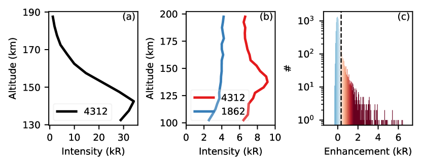
Figure 1: Examples of MAVEN/IUVS limb scans showing the thermospheric altitutde profiles of co2uvd emission (a) and Ly-${\rm\alpha}$ emissions (b). The Ly-${\rm\alpha}$ emissions show both a proton aurora case (red) and a non-proton aurora case i.e. the background dayglow emission (blue). The proton aurora profile shows the characteristic enhancement around 120 – 150 km altitudes. The legend shows the orbit number for each profile. Distribution of the Ly-${\rm\alpha}$ enhancements within the data considered is shown in (c).

We use remote sensing and in-situ data from MAVEN between October 2014 — April 2022 for developing an ANN model of the observed Ly-$\alpha$ emission altitude profiles. The data considered here covers almost four Martian years. All MAVEN data is publicly accessible at the MAVEN Science Data Center https://lasp.colorado.edu/maven/sdc/public/. Details of the analyzed data are as follows.

2.1 IUVS Limb-Scan Observations

MAVEN/IUVS is a remote-sensing UV spectrograph monitoring the state of the Mars’ upper atmosphere (110 – 225 km). The IUVS wavelength range covers the FUV (110 – 190 nm) and MUV (180 – 340 nm) ranges. IUVS is thus sensitive to, among other emissions, Ly-$\alpha$ (121.3 nm) which is the focus of this study on proton auroras as well as ${\rm CO_{2}}$+UV Doublet band (288.3 nm and 289.6 nm, co2uvd) which we use as a proxy for the ${\rm CO_{2}}$ atmosphere density (Deighan et al., 2018). We use the publicly available Level 1C processed data products. During periapsis passes, IUVS operates in the limb-scan mode, when it records the altitude emission profiles between 100 – 220 km (McClintock et al., 2015). Typically, 12 such scans are recorded for each periapsis passing segment lasting $\rm{\sim~{}23~{}min}$.

We only use limb-scan profiles that provide emissions for the full altitude range between 100 – 200 km for Ly-$\rm{\alpha}$ and 130 – 190 km for co2uvd. These altitude ranges are chosen to minimize the exclusion of limb-scan observations because of any missing data at lower or higher altitudes and still cover the region of Mars’ thermosphere relevant for this study. The proton auroras in Ly-$\rm{\alpha}$ altitude scans are identified as an enhancement of emission intensity between 120 – 150 km. Following Hughes et al. (2019), we quantify the emission enhancement using a measure EM defined as the difference between the second highest intensity in the peak altitude range and the median value between 160 – 190 km range. Figure 1a shows a sample co2uvd emission profile and Figure 1b shows samples of Ly-${\rm\alpha}$ profiles for a non-proton aurora observation and a proton aurora observation. The latter shows a marked enhancement of Ly-${\rm\alpha}$ emission in the peak altitude range compared to the characteristic flat dayglow profile in the former. Also, following (Hughes et al., 2019), we define an observation to be a proton aurora if EM is exceeds ${\rm 0.5\sigma}$ than the mean EM, ${\rm\sigma}$ being the standard deviation of EMs in the data. Figure 1c shows the distribution of the enhancements across the data considered for the analysis, with the threshold highlighted by the dashed black line. Hughes et al. (2019) showed that the occurrence rate of proton auroras primarily depends on ${\rm L_{s}}$ and SZA. We, therefore, include these in our analysis along with other measurements latitude (lat), longitude (lon), and local time (lt) for each limb scan.

2.2 MAVEN in-situ measurements of protons and magnetic field

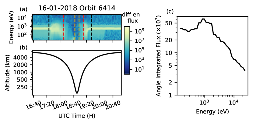
Figure 2: Example of MAVEN/SWIA measurements for a sample orbit showing the variation in the proton energy spectra (a) and the MAVEN altitude (b). The bow-shock (black) and magnetic pile-up boundaries (red) marked by the dashed lines are from Trotignon et al. (2006). The region within the dashed yellow line shows observations below 250 km identified as the thermosphere region in our analysis. (c) shows the energy spectra of protons within the thermosphere region as per Halekas et al. (2015). The peak indicates the penetrating solar wind proton population with the characteristic energy $\sim$ 1 keV.

MAVEN measures in-situ properties of plasma and radiation it encounters in its flight. We use various in-situ measurements from Solar Wind Ion Analyser (SWIA) (Halekas et al., 2015) and MAGnetometer (MAG) (Connerney et al., 2015) onboard MAVEN to characterise the influence of solar wind protons and magnetic fields on proton auroras. The details are as follows.

In its orbit, MAVEN samples plasma from different regions of the magnetosphere — solar wind upstream of bow shock (SW), magnetosheath (MS) and thermosphere (TH). We identify measurements within SW using the algorithm from Halekas et al. (2017a). We use bow shock and magnetic pile-up boundary positions from Trotignon et al. (2006) to identify measurements within the MS. Finally, we use observations taken below 250 km as TH in-situ observations. Depending on the altitude, MAVEN does not always sample plasma from SW in each orbit; we only include the orbits in our analysis for which MAVEN samples observations from SW. Figure 2a shows the identified positions of bow shock, magnetic pile-up boundary and TH regions from the SWIA energy spectra for protons for a sample orbit. For SW and MS regions, we use the average values of proton and in-situ measurements over an orbit. For TH region, we divide all observations within an orbit in 12 equal parts (approximately one for each limb scan) and take the average values from each part. This facilitates characterising local changes in proton aurora emissions, if present, within an orbit. Each of the 12 parts is marked by corresponding average SZA and altitude.

Table 1: List of MAVEN/SWIA and MAVEN/IUVS observations used as input features for modelling Ly-$\alpha$ altitude profiles also observed by MAVEN/IUVS. MAVEN/SWIA observations are sampled from Upstream solar wind (SW), magnetosheath (MS) and thermosphere (TH) regions, identified as described in Figure 2.

SWIA In-situ Measurements		IUVS Remote Sensing Measurements
Upstream Solar Wind (SW)	Thermosphere (TH:insitu)	Thermosphere (TH:co2uvd)
IMF Clock Angle ($\mathrm{IMF_{clock}}$)	Total crustal magnetic field ($\mathrm{B_{tot,cr}}$)	co2uvd altitude profile
IMF Cone Angle ($\mathrm{IMF_{cone}}$)	Radial crustal magnetic field ($\mathrm{B_{r,cr}}$)	Thermosphere (TH:res ms.)
MSE-X Proton Speed ($\mathrm{{Vmse}_{x,SW}}$)	Azimuthal crustal magnetic field ($\mathrm{B_{\phi,cr}}$)	solar season ($\mathrm{L_{s}}$)
Proton temperature ($\mathrm{{T}_{SW}}$)	Polar crustal magnetic field ($\mathrm{B_{\theta,cr}}$)	local time (lt)
Proton density ($\mathrm{{\rho}_{SW}}$)	Total magnetic field ($\mathrm{B_{tot,TH}}$)	solar zenith angle (SZA)
Magnetosheath (MS)	Radial magnetic field ($\mathrm{B_{r,TH}}$)	Latitude (lat)
Total magnetic field ($\mathrm{B_{tot,MS}}$)	Azimuthal magnetic field ($\mathrm{B_{\phi,TH}}$)	Longitude (lon)
Radial magnetic field ($\mathrm{B_{r,MS}}$)	Polar magnetic field ($\mathrm{B_{\theta,TH}}$)
Azimuthal magnetic field ($\mathrm{B_{\phi,MS}}$)	Elevation angle ($\mathrm{\theta_{TH}}$)
Polar magnetic field ($\mathrm{B_{\theta,MS}}$)	Azimuth angle ($\mathrm{\phi_{TH}}$)
Elevation angle ($\mathrm{\theta_{MS}}$)	MSE-X Proton Speed ($\mathrm{{Vmse}_{x,TH}}$)
Azimuth angle ($\mathrm{\phi_{MS}}$)	MSE-Y Proton Speed ($\mathrm{{Vmse}_{y,TH}}$)
MSE-X Proton Speed ($\mathrm{{Vmse}_{x,MS}}$)	MSE-Z Proton Speed ($\mathrm{{Vmse}_{z,TH}}$)
MSE-Y Proton Speed ($\mathrm{{Vmse}_{y,MS}}$)	Proton temperature ($\mathrm{{T}_{TH}}$)
MSE-Z Proton Speed ($\mathrm{{Vmse}_{z,MS}}$)	Proton density ($\mathrm{{\rho}_{TH}}$)
Proton temperature ($\mathrm{{T}_{MS}}$)	Solar Zenith Angle ($\mathrm{{SZA}_{TH}}$)
Proton density ($\mathrm{{\rho}_{MS}}$)	Altitude ($\mathrm{{ALT}_{TH}}$)
	Penetrating proton energy spectra (TH:en spec.)

Proton auroras are affected by the solar wind protons, which are monitored by MAVEN/SWIA. SWIA measures proton flux over an energy range of 10 eV – 5 keV, providing information about proton energies, velocities and temperatures. We convert the velocities provided in Mars-centered Solar Orbital (MSO) coordinate system to Mars Solar Electrical (MSE) coordinate system. In MSE, x points anti-parallel to the solar wind velocity ($\bf{v}_{SW}$), z points in the motional electric field direction $\bf{E}_{SW}=-\bf{v}_{SW}\times\bf{B}_{SW}$ and y completes the right handed system. For TH region, we explicitly include the spectrum of penetrating ENAs converted to protons (Halekas et al., 2015), which typically shows a peak of flux at the characteristic solar wind energy ${\rm 1~{}keV}$, as an additional input to the model. An example of the spectrum is shown in Figure 2c.

In order to study the influence of the magnetic field on proton aurora, we use in-situ measurements of magnetic fields from MAG onboard MAVEN (Connerney et al., 2015). The magnetic-field measurements are provided in MSO coordinate system. For SW measurements, we convert magnetic fields to solar wind clock angle (${\rm B_{clock}}$) and cone angle (${\rm B_{cone}}$) that characterise the direction of Interplanetary Magnetic Field (IMF). For MS and TH regions, we decompose the measurements into the magnitude, elevation angle and azimuth angle (Hara et al., 2018). The elevation angle (${\rm\theta}$) measures how radial (${\rm\pm~{}90\degree}$) or horizontal the magnetic field is. The azimuth angle (${\rm\phi}$) measures how east (${\rm 0\degree}$) or north (${\rm 90\degree}$) the horizontal magnetic field is. In addition to these, we also use the in-situ magnetic-field components in spherical co-ordinate system centered at Mars ${\rm B_{r}}$, ${\rm B_{\theta}}$, and ${\rm B_{\phi}}$.

Proton auroras may have preferential occurrence relative to crustal magnetic fields of Mars. These fields are extensively modeled using MAVEN and Mars Global Surveyor (MGS) (Acuña et al., 2001) observations. Here, we use a publicly available model from Gao et al. (2021), that estimates the crustal field with a spatial resolution of ${\rm\sim 200~{}km}$ and can model MAVEN observations based on these crustal fields within ${\rm\sim nT}$ of the true observations. We use total crustal magnetic field magnitude ${\rm B_{tot,crustal}}$ and spherical co-ordinate system components ${\rm B_{r,crustal}}$, ${\rm B_{\theta,crustal}}$ and ${\rm B_{\phi,crustal}}$ for our analysis. All observations used as the ANN input are listed in Table 1.

3 Methods

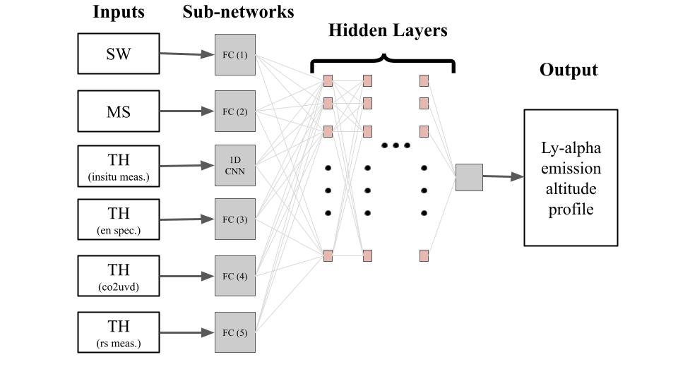
Figure 3: The Artificial Neural Network (ANN) Architecture: The ANN takes in SWIA in-situ measurements of proton properties and magnetic fields from upstream solar wind (SW), magnetosheath (MS) and thermosphere (TH) regions, as well as remote sensing geometry measurements of each IUVS limb scan. These input features are summarised in Table 1. Fully connected (FC) or 1D Convolutional Neural Network (CNN) sub-networks process the individual set of input features and yield an abstract representation. These representations are further processed by layers of fully connected neurons (hidden layers) to obtain the observed Ly-${\rm\alpha}$ altitude profile of each IUVS limb scan as the output. The details of the FC and 1D-CNN sub-networks, hidden layers and the output layer are given in the main text.

We build an ANN model for the Ly-${\rm\alpha}$ intensity altitude profiles observed by MAVEN/IUVS in each periapsis limb scan using MAVEN/SWIA in-situ observations of proton energies, velocity, temperature and magnetic fields, modelled crustal magnetic fields and MAVEN/IUVS observations of co2uvd altitude profiles as well as SZA, ${\rm L_{s}}$, latitude, longitude and local time for each limb scan (see Table 1). The ANN architecture is shown in Figure 3.

3.1 Artificial neural network architecture

An ANN is a function ${\rm\bf{Y}=f_{\theta}\left(\bf{X}\right)}$, where ${\rm\bf{X}}$ are the inputs, ${\rm\bf{Y}}$ is the modelled output and ${\rm\theta}$ are the parameters — weights and biases — of the artificial neurons in the network. Each artificial neuron outputs ${\rm\sigma\left(\bf{w}\cdot\bf{x}+\bf{b}\right)}$, where ${\rm\bf{x}}$ is the output from the previous layer (or the input features), ${\rm\bf{w}}$ and ${\rm\bf{b}}$ are the weights and biases of the neuron, and ${\rm\sigma}$ is an activation function Hastie et al. (2001). A fully connected (FC) layer of neurons is connected to all neurons (or the inputs) in the previous layer. Layers in a convolution neural network (CNN) are made up of convolution filters, comprising a set of neurons with same weights and biases, that sequentially process outputs from the previous layer (or the inputs) to output feature maps. Convolutional layers are typically used to process images or tabular data.

In this work, the input features consist different types of observations — orbit average values (SW and MS), average time series of measurements for each orbit (TH:insitu meas.), energy spectra (TH:en spec.), the co2uvd altitude profiles (TH:co2uvd) and other remote sensing measurements (TH:rs meas.). Hence, we use different sub-networks to individually process different inputs and obtain a homogeneous abstract representation that is further processed by several FC layers (hidden layers) to yield the output. All inputs except TH:insitu meas. are 1D features and are processed by a FC sub-network with identical architecture. TH:insitu meas. are 2D tabular inputs with 12 average values of each features spaced equally in time during the periapsis scan and are processed by a 1D-CNN. The details of sub-networks FC and 1D-CNN, and FC hidden layers are as follows.

• FC sub-network: This is made up of three FC layers including the output layer. First and second layers have 128 and 256 neurons respectively while the output layer has 64 neurons. The number of inputs are different for different input groups as listed in Table 1. All neurons have the sigmoid activation that gives an output value between 0 and 1 Hastie et al. (2001).

• 1D-CNN sub-network: This comprises of two 1D convolutional layers and one FC layer of neurons. The first convolution layer has 32 filters, while the second convolution layer has 64 filters. The output of the second convolution layer is flattened and fed into a FC layer with 128 neurons. The 1D-CNN operation takes place with a convolution filter of kernel size one and stride one, sliding sequentially over the time series values of each feature, picking up identical patterns from measurements across different times, correlated with the Ly-${\rm\alpha}$ intensity and enhancements. Each neuron in the sub-network has the sigmoid activation.

• Hidden layers: The abstract representations of input features are concatenated (vector with length ${\rm 64\times 5+128=448}$) and fed into a network of three FC hidden layers with 1024, 512 and 256 neurons respectively. Each neuron in the hidden layers has the sigmoid activation.

• Output layer: The output of the hidden layers (length=256) is fed into the output layer with 20 neurons modeling the observed Ly-${\rm\alpha}$ emission intensity profile between 100 – 200 km binned into 20 equally spaced altitude bins. All neuorns in the output layer also have the sigmoid activation function.

3.2 Training

We split the available MAVEN data between October 2014 and April 2022 into three parts for training (60%), validation (20%) and test (20%). The training set data is used to train the ANN i.e. obtain the values of weights and biases that accurately model the output. The validation set data is used to ensure that the model is not overfitting and its performance is generalisable by tuning the hyperparameters (discussed below). A well trained ANN learns concrete patterns from the data to model the output and generalises to yield good performance on the test set, which is a final test of an ANN model.

Proton aurora observations in different limb scans from an orbit are correlated (Hughes, 2021) and, therefore, mixing limb-scan observations from the same orbit in training, validation and test would result in an artificially high performance. Hence, we first randomly split the orbits in the given ratio and all limb scans from each orbit are then included in the respective set. The total number of orbits for training, validation and test data are 1326, 442, and 443 respectively. The total number of limb scans for training, validation and test data are 7178, 2382, and 2384 respectively. Note that only those orbits are included in our analysis for which MAVEN samples any upstream solar wind observation.

During training, all samples from the training data are fed into the ANN. For each sample, the ANN returns an output Ly-${\rm\alpha}$ emission intensity altitude profile ${\rm\bf{Y}}$ that is compared with the true observed profile ${\rm\bf{Y_{true}}}$ and a loss function ${\rm L(\bf{Y},\bf{Y}_{true})}$ is computed. The ANN weights and biases are then modified using a stochastic gradient descent to yield a minimum value for the loss function as the training progresses. For regression problems, such as the one considered here, the most commonly used loss function is a mean squared error (MSE) defined as,

$$\mathrm{L_{MSE}\left(\bf{Y},\bf{Y}_{true}\right)=\frac{1}{N}\sum_{i}^{N}\frac{1}{M}\sum_{j}^{M}\left(Y_{i}^{j}-Y_{true,i}^{j}\right)^{2},}$$ (1)

where N is the total number of samples, M=20 is the number of altitude bins and Y’s (${\rm Y_{true}}$’s) are the corresponding Ly-${\rm\alpha}$ intensity values for the modelled (true) scans. The MSE loss function does not explicitly aid the ANN to accurately model the shape of the individual intensity profile, including the characteristic peak for proton auroras. Rather it only aids in reducing the overall mean square error in the intensities. To accurately model the shape, we additionally use structural similarity index (SSIM) defined as,

$$\mathrm{SSIM\left(\bf{Y},\bf{Y}_{true}\right)=\frac{\left(2\mu_{\rm\bf{Y}}\mu_{\rm\bf{Y}_{true}}+C_{1}\right)\left(2\sigma_{\rm\bf{Y}\bf{Y}_{true}}+C_{2}\right)}{\left({\mu^{2}_{\rm\bf{Y}}}+\mu^{2}_{\rm\bf{Y}_{true}}+C_{1}\right)+\left(\sigma^{2}_{\rm\bf{Y}}+\sigma^{2}_{\rm\bf{Y}_{true}}+C_{2}\right)},}$$ (2)

where $\rm{\mu}$’s are the means and ${\rm\sigma^{2}}$’s are the variances of ${\rm\bf{Y}}$ and ${\rm\bf{Y}_{true}}$ respectively and $\sigma_{\rm\bf{Y}\bf{Y}_{true}}$ is the covariance. ${\rm C_{1}}$ and ${\rm C_{2}}$ are constants. The SSIM value ranges between 0 and 1, with the latter meaning that the two profiles are identical. The SSIM loss is therefore defined as,

$$\mathrm{L_{SSIM}\left(\bf{Y},\bf{Y}_{true}\right)=1-SSIM\left(\bf{Y},\bf{Y_{true}}\right).}$$ (3)

The EM for each profile provides an additional constraint that can be used for modelling. We use the mean squared error for EM,

$$\mathrm{L_{MSE,EM}\left(\bf{Y},\bf{Y}_{true}\right)=\frac{1}{N}\sum_{i}^{N}\left(EM\left(Y\right)_{i}-EM\left(Y_{true}\right)_{i}\right)^{2},}$$ (4)

as a third loss function for training. The complete loss function used for training is a weighted sum of the three loss functions

$$\mathrm{L\left(\bf{Y},\bf{Y}_{true}\right)=L_{MSE}\left(\bf{Y},\bf{Y}_{true}\right)+\lambda_{1}\cdot L_{SSIM}\left(\bf{Y},\bf{Y}_{true}\right)+\lambda_{2}\cdot L_{MSE,EM}\left(\bf{Y},\bf{Y}_{true}\right)},$$ (5)

where weight coefficients ${\rm\lambda_{1}}$ and ${\rm\lambda_{2}}$ are hyperparameters used for balancing contributions of the different loss function terms.

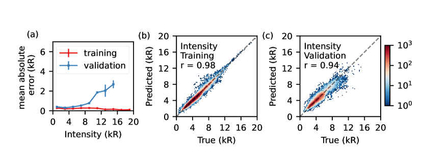
Figure 4: Performance of the ANN: (a) Mean absolute error in the predicted intensity as a function of true intensity binned in 10 equal sized bins. The error bars indicate 1${\rm\sigma}$ standard error. (b) & (c) Heatmaps showing the population of predicted intensity samples binned in 2D as per true and predicted intensities for training and validation sets respectively. Note that the bins lying closer to the diagonal (dashed line) indicate accurate predictions. The corresponding Pearson correlation values (r) are also noted.

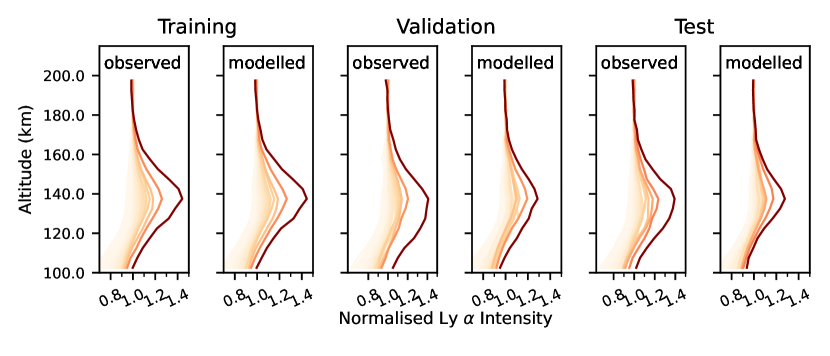
Figure 5: Summary of reconstructed Ly-${\rm\alpha}$ intensity altitude profiles for the training, validation and test data. Each profile is a mean profile obtained from a population of profiles binned in percentile bins of the peak intensity enhancements. Darker color indicates increasing enhancement value. Each profile is normalised by mean intensity values between altitude range 160 – 200 km (Hughes et al., 2019).

Since the ANN learns empirically from the data it is important to have the training data free from any biases with respect to the modeled phenomena i.e. in this case Ly-${\rm\alpha}$ intensity and proton aurora enhancements. As shown in Figure 1c, the number of limb scan profiles decrease significantly with increasing enhancement. We bin the Ly-${\rm\alpha}$ profiles in training data as per EM and repeat the number of samples, i.e. oversample, the data in bins with high EM values to match the number in the lowest enhancement bin. Thus, the distribution of Ly-${\rm\alpha}$ profiles to be modelled in the training data is uniform with respect to EM.

Apart from weights and biases, the ANN model also has hyperparameters that are important for training the model and minimising the loss function. These include the learning rate i.e. the step size for the stochastic gradient descent, batch size i.e. the number of samples used to calculate the gradients for updating weights and biases, the parameters ${\rm\lambda_{1}}$ and ${\rm\lambda_{2}}$ for the loss function. We monitor the performance of model on the validation data to tune the values of these hyperparameters. We implement the ANN model using pytorch (Paszke et al., 2019).

4 Results

4.1 Accuracy of the modelled proton auroras

We use mean absolute error of the modelled Ly-$\alpha$ intensities, Pearson correlation between true and modelled intensities as well as EM values for each true and modelled profile for quantifying the accuracy and performance of the ANN model. Mean absolute error and a comparison of true and modelled intensities are shown in Figure 4. Panel (a) shows mean absolute error in the modelled intensities, calculated for the populations of increasing true intensity values split into bins. For the intensities up to 10 kR, the mean absolute error remains very low $<$ 1 kR. Although the mean absolute error increases as the true intensity values increase, it does not exceed a maximum of 3 kR. Panel (b) and (c) show a heatmap comparison of true and modelled intensity values, with a significant majority of the samples lying adjacent to the diagonal. The Pearson correlation yields high values, 0.98 and 0.94 for training and validation respectively. Similar to the true Ly-$\alpha$ altitude profiles, we obtain the EM values for the modelled profiles. The EM values from true and modelled profiles yield a Pearson correlation of 0.95 and 0.65 respectively. The test data yields Pearson correlation values of 0.95 and 0.63 for the intensities and EMs respectively.

Hughes (2021) developed a simple linear regression fit for obtaining Ly-$\alpha$ enhancement averaged over an orbit using only the flux of penetrating protons measured by SWIA. They developed three different models for three different scenarios — nominal conditions, extreme solar events, and events during high dust activity. They obtained ${\rm R^{2}}$ values 0.87, 0.61, 0.43 for these three scenarios respectively. Compared to their results our comprehensive ANN model, that works for all scenarios, yields a far superior ${\rm R^{2}}$ value for orbit averaged EMs as 0.96 for the training data. Our model also generalises reasonably well to the validation and test data yielding an ${\rm R^{2}}$ of 0.67 and 0.57 respectively. Thus, the ANN model presented here performs better than a baseline model of a uni-variate linear regression using only penetrating proton flux.

Figure 5 shows a direct comparison of mean Ly-$\alpha$ altitude profiles, binned for each percentile population as per EM, for the training, validation and test data respectively. The ANN model accurately reproduces the enhancement shape of the profiles, between altitudes 120 – 150 km, as expected. For the training data the modelled and observed profiles conform closely to each other across all percentile bins. For the validation and test data, the modelled profiles produce systematically lower peak intensities compared to the true observations for the highest percentile bin. For the lower percentile bins, the observed and modelled profiles compare reasonably well.

4.2 SHAP Values: Identifying important features

Table 2: Ranking of inputs: sum of SHAP values of all measurements in each input group representing an average (unsigned) contribution to a Ly-$\alpha$ altitude profile observation.

Input Group	Avg. SHAP Value (kR)
TH:rs meas.	1.13
TH:co2uvd	0.86
TH:insitu meas.	0.54
TH:en spec.	0.22
SW	0.17
MS	0.08

Table 3: Selection of important features from upstream solar wind (SW), meagnetosheath (MS) and thermosphere (TH) insitu measurements as well as TH remote sensing geometry measurements. The table lists unsigned SHAP values (normalised for each group by the maximum value) and their Pearson correlation (r) with the corresponding measurements.

TH: res meas.			TH: insitu meas.			MS
Feature	Norm. SHAP	$\mathrm{\mathbf{r_{shap}}}$	Feature	Norm. SHAP	$\mathrm{\mathbf{r_{shap}}}$	Feature	Norm. SHAP	$\mathrm{\mathbf{r_{shap}}}$
$\mathrm{L_{s}}$	0.14	0.89	$\mathrm{B_{tot,cr}}$	0.01	-0.52	$\mathrm{B_{tot,MS}}$	0.01	-0.17
lat	0.16	-0.92	$\mathrm{B_{r,cr}}$	0.02	0.15	$\mathrm{B_{r,MS}}$	0.06	-0.13
lon	0.00	0.32	$\mathrm{B_{\theta,cr}}$	0.01	-0.05	$\mathrm{B_{\theta,MS}}$	0.13	0.24
lt	0.35	-0.74	$\mathrm{B_{\phi,cr}}$	0.03	0.06	$\mathrm{B_{\phi,MS}}$	0.00	-0.26
SZA	0.34	-0.90	$\mathrm{{Vmse}_{x,TH}}$	0.04	0.00	$\mathrm{\mathbf{\theta_{MS}}}$	0.13	-0.17
SW			$\mathrm{{Vmse}_{y,TH}}$	0.03	-0.30	$\mathrm{\phi_{MS}}$	0.06	0.21
Feature	Norm. SHAP	$\mathrm{\mathbf{r_{shap}}}$	$\mathrm{{Vmse}_{z,TH}}$	0.01	-0.34	$\mathrm{{Vmse}_{x,MS}}$	0.23	-0.21
$\mathrm{IMF_{clock}}$	0.09	0.79	$\mathrm{{T}_{TH}}$	0.10	-0.37	$\mathrm{{Vmse}_{y,MS}}$	0.00	-0.14
$\mathrm{IMF_{cone}}$	0.15	-0.79	$\mathrm{{\rho}_{TH}}$	0.02	-0.10	$\mathrm{{Vmse}_{z,MS}}$	0.03	0.20
$\mathrm{{Vmse}_{x,SW}}$	0.07	-0.77	$\mathrm{B_{tot,TH}}$	0.02	0.14	$\mathrm{{T}_{MS}}$	0.28	-0.11
$\mathrm{{T}_{SW}}$	0.20	0.81	$\mathrm{B_{r,TH}}$	0.01	0.01	$\mathrm{{\rho}_{MS}}$	0.06	-0.05
$\mathrm{{\rho}_{SW}}$	0.49	0.35	$\mathrm{B_{\theta,TH}}$	0.08	-0.01
			$\mathrm{B_{\phi,TH}}$	0.03	0.45
			$\mathrm{\theta_{TH}}$	0.09	-0.25
			$\mathrm{\phi_{TH}}$	0.10	0.06
			$\mathrm{{SZA}_{TH}}$	0.30	-0.06
			$\mathrm{{ALT}_{TH}}$	0.09	0.10

Complex ML models such as neural networks, although highly efficient and accurate in learning from large high-dimensional datasets, are notoriously difficult to interpret. An interpretation or explanation of a trained ANN model, however, is highly desirable; first and foremost to gain a confidence in applying the model to new data, and subsequently, if possible, to uncover new patterns in the data, hitherto unknown because of their complicated relationship with the modelled phenomena. Over the last decade, a number of such interpretation/explanation methods have been developed (Simonyan et al., 2013; Zeiler & Fergus, 2014; Sundararajan et al., 2017; Selvaraju et al., 2017; Shrikumar et al., 2017). Additive feature attribution methods are a class of explanation models that can be written in the form of a linear function of binary variables that indicate presence/absence of the model inputs. Shapley value, from cooperative game theory, are useful for quantifying impact of each feature on the model output. Lundberg & Lee (2017) developed SHapley Additive exPlanations (SHAP), based on Shapley values, as a unified measure of feature importance for the class of additive feature attribution methods satisfying a number of desirable properties. SHAP values have proven widely successful and are now a state-of-the-art for explaining a ML model output in terms of contributions of its input features. We use the publicly available python library (https://github.com/shap/shap) to compute SHAP values (Deep SHAP) for our trained ANN model.

For a given model output, SHAP value for each input is the contribution of the input to the difference between the model output and an expected model output for a set of reference inputs. The sum of SHAP values for all inputs, thus, adds up to the difference between the given model output and expectation value of the reference model output. Here, we use the training data inputs as a reference for calculating the SHAP values. Since we are interested in understanding the relationship between the inputs and the Ly-$\alpha$ enhancement during proton aurora, we consider mean SHAP values for the Ly-$\alpha$ intensities between altitudes 120 – 150 km. SHAP values here are measured in kR, same as the intensities. Table 2 lists an average unsigned SHAP value for each group of input features over the training and validation data. As the table shows, TH:res meas. and co2uvd intensity profiles that serve as a proxy for the ${\rm CO_{2}}$ atmosphere contribute most to the model output on average, while the MS measurements contribute the least. In the following, we analyse SHAP values of important features from each input group in detail.

4.2.1 In-situ Measurements

SHAP values for the TH remote sensing and insitu measurements are the highest and third highest respectively. Table 3 lists unsigned SHAP values for these features as well as for SW and MS insitu measurements. The SHAP values are normalised by the maximum unsigned value for the respective group. For the most significant features, the normalised SHAP value exceeds an equal contribution value of ${\rm 1/N}$ where N is the total number of features from the respective group. We also calculate Pearson correlation (r) between the SHAP values and the measured values of the features. High values of r indicate a strong linear relationship between the SHAP value and the feature, suggesting the existence of a definite pattern associated with the Ly-$\alpha$ enhancements. The significant normalised SHAP values and/or a relatively high ${\rm r}$ helps us identify input features from these groups, with definite patterns correlated to the modelled Ly-$\alpha$ intensities. Figure 6 shows the distribution of SHAP values for these selected features, while additional features also contributing significantly for each group are presented in the Appendix.

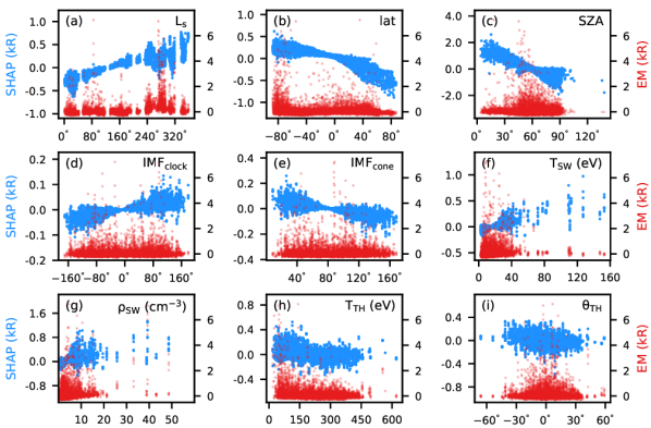
Figure 6: Distribution of SHAP values (blue) vs measurements of the important input features from solar wind (SW) and thermosphere (TH) insitu measurements as well as TH remote sensing geometry measurements as identified in Table 3. The distribution of Ly-$\alpha$ enhancement (EM) corresponding to each measurement is also shown (red).

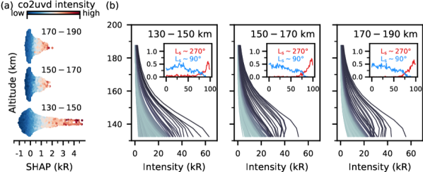
Figure 7: SHAP values for the co2uvd altitude profile input. Panel (a) show the SHAP values for co2uvd intensity values grouped in three altitude regions, with the colorbar showing the scale of intensities. Panel (b) shows the mean co2uvd altitude profiles for 100 percentile bins ordered by SHAP values of each altitude range. The darker color corresponds to higher SHAP values. The inset plots show the fraction of observations in each percentile bin corresponding to ${\rm L_{s}=270\degree\pm 25\degree}$ and ${\rm L_{s}=90\degree\pm 25\degree}$.

Table 4: Pearson correlation (r) of flux of penetrating protons (observed within the thermosphere, TH) at different energies measured by MAVEN/SWIA, with the flux measured at energy 964.61 eV that is closest to the typical solar wind energy 1 keV. The energies are grouped as per their correlation values.

Energy (eV)	r	Energy (eV)	r
23245.0	0.13	1720.4	0.64
20114.0	0.13	1488.7	0.64
17406.0	0.15	1288.2	0.86
15062.0	0.15	1114.7	0.86
13033.0	0.17	964.61	1.00
11278.0	0.17	834.71	1.00
9759.4	0.19	722.3	0.91
8445.1	0.19	625.03	0.91
7307.9	0.21	540.86	0.66
6323.7	0.21	468.02	0.66
5472.1	0.25	405.0	0.53
4735.2	0.25	350.46	0.53
4097.5	0.29	303.26	0.74
3545.7	0.29	262.42	0.74
3068.2	0.42	227.08	0.77
2655.0	0.42	196.5	0.77
2297.5	0.50	170.04	0.73
1988.1	0.50	147.14	0.73

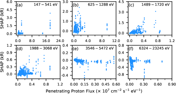
Figure 8: Distribution of SHAP values for penetrating proton flux for modeling Ly-$\alpha$. The penetrating proton flux are grouped into different energy bins as per the Pearson correlation of the flux with the flux at $\sim$ 1 keV (see Table 4).

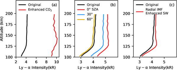
Figure 9: Simulating Ly-$\alpha$ response using the trained ANN model on test data samples. The original altitude profiles are mean profiles of the lowest EM percentile bin population. Panel (a) shows the effect of an enhanced ${\rm CO_{2}}$ atmosphere in terms of enhanced co2uvd intensities. Panel (b) shows the effect changing SZAs. Panel (c) shows the influence of changing the solar wind conditions to southward, radial IMF with clock and cone angles of ${\rm 150\degree}$ and ${\rm 5\degree}$ respectively, as well as enhanced temperature and density.

${\rm L_{s}}$, Latitude and SZA for the geometry of remote sensing measurements of Ly-$\alpha$ (and also co2uvd) are the most important features from TH remote sensing measurements. As shown in Figure 6a, the SHAP values increase approximately linearly with increasing ${\rm L_{s}}$ and reach a maximum of ${\rm\sim 0.5~{}kR}$ around southern summer solstice, consistent with the highest occurrence rates of proton auroras during that season (Hughes et al., 2019). From Panel (b), the SHAP values for southern hemisphere latitudes are highest ${\rm\sim 0.2~{}kR}$, while those for the northern hemisphere latitudes are lowest up to ${\rm\sim-0.8~{}kR}$. The plot also shows that the highest enhancements occur at southern hemisphere latitudes, most likely biased by the seasonal dependence discussed above.

Figure 6c shows that the SHAP values are highest ${\rm\sim 2.0~{}kR}$ for low SZAs ${\rm\sim 0\degree}$ and decrease monotonically with increasing SZAs. This is consistent with the known proton aurora mechanism, as being a dayside phenomena, the enhancements are expected to be maximum for the lowest SZA (Hughes et al., 2019). The proton aurora enhancements (also shown in the figure) are, however, found to be highest for mid SZAs ${\rm\sim 45\degree}$. This discrepancy is mainly due to the observation bias of the proton aurora occurrence being maximum during southern summer for which the low SZA Ly-$\alpha$ observations are few. The ANN model here learns the true expected relationship as the Ly-$\alpha$ intensities for different limb scans within a single orbit also decrease monotonically as a function of SZA (Hughes, 2021; He et al., 2023).

Distribution of SHAP values for the most significant SW measurements ${\rm IMF_{clock}}$, ${\rm IMF_{cone}}$, ${\rm T_{SW}}$ and ${\rm\rho_{SW}}$ are shown in Figure 6, Panels (d), (e), (f) and (g) respectively. The SHAP values are positive and have an increasing trend for positive and increasing ${\rm IMF_{clock}}$ angles with maximum SHAP values occurring at ${\rm\sim 180\degree}$ corresponding to a southward ${\rm B_{SW,z}}$. Although, the magnitude of SHAP values is only up to ${\rm\sim 0.1~{}kR}$ i.e. not significantly high. SHAP values are also increasing and positive for decreasing ${\rm IMF_{cone}}$ angles, with the maximum values ${\rm\sim 0.2~{}kR}$ for radial IMFs. The double peak structure of enhancements with respect to ${\rm IMF_{clock}}$ and ${\rm IMF_{cone}}$ angles has been reported before by Hughes (2021), and is also apparent in the enhancement distributions shown in the both figures. Here, however, the SHAP values suggest that southward and radial IMFs are more important for the increased peak Ly-$\alpha$ intensities. The SHAP values also generally increase with increasing solar wind temperatures and densities as expected.

Panels (h) and (i) show the SHAP values for TH temperature ${\rm T_{TH}}$ and elevation angle ${\rm\theta_{TH}}$, both showing a slightly decreasing trend with an increase in the respective measurement values. Lower i.e. ${\rm\theta_{TH}\sim-90\degree}$ imply a downward radial field, offering the least resistance to radially downward moving penetrating protons and thus favorable for proton auroras. The higher SHAP values for a population of protons with lower ${\rm T_{TH}\sim 50~{}eV}$ values is counter-intuitive, although an increased enhancement is also seen with these lower ${\rm T_{TH}}$ values as shown in the figure. This low TH temperature proton population may correspond to de-excited and de-energized solar wind penetrating protons via repeated charge exchange and electron capture collisions with the ${\rm CO_{2}}$ atmosphere. Table 4 lists correlations between the penetrating proton flux at solar wind energy ${\rm\sim 1~{}keV}$ and other energies and it is interesting to note relatively high Pearson correlation values for the lowest energies, roughly consistent with the enhancements and SHAP values observed for low ${\rm T_{TH}}$.

4.2.2 CO2UVD Altitude Profiles

We divide the co2uvd intensity profiles in three groups based on altitudes — 130 – 150 km that overlap with the Ly-$\alpha$ peak altitudes, and higher altitudes 150 – 170 km and 170 – 190 km. For all three groups, the SHAP values are higher corresponding to the higher intensities at the respective altitudes as shown in Figure 7a. The lowest altitude group yields the highest SHAP values up to $\sim$ 5 kR as expected. The higher altitude groups 150 – 170 km and 170 – 190 km yield SHAP values up to $\sim$ 2 kR. Figure 7b shows average altitude profiles for 100 percentile bins ordered by the SHAP values for the three altitude groups. The highest percentile bins for all groups show average co2uvd profiles with higher overall intensities at all altitudes, but particularly at the respective altitude range. The inset plot shows the fraction of samples within each percentile bin approximately corresponding to southern summer solstice (${\rm L_{s}\sim 270\degree}$) and southern winter solstice (${\rm L_{s}\sim 90\degree}$). The fraction of profiles from southern summer are higher for the highest percentile bins 75-100 in all three cases, whereas the fraction of profiles from southern winter systematically decrease to 0 for the higher altitude range 150 – 170 km and 170 – 190 km. Thus, intensities at higher altitudes are important for modelling the Ly-$\alpha$ intensities around the southern summer solstice when Mars is closest to the Sun, and hence its ${\rm CO_{2}}$ atmosphere is inflated.

4.2.3 Penetrating Proton Energy Spectra

The penetrating proton population is identified by a peak at the characteristic solar wind proton energy ${\rm\sim 1~{}keV}$ (Halekas et al., 2015). We find that the penetrating proton fluxes at other energies are also strongly correlated with the flux at ${\rm\sim 1~{}keV}$ as shown in Table 4. We divide the energy spectra into six energy ranges depending on the degree of correlation with the typical solar wind energy. The SHAP values as a function of the total flux for these energy ranges are shown in Figure 8. We find that the SHAP values are highest up to ${\rm\sim 2.0~{}kR}$ for the energy range containing 1 keV (Panel b), and increase sharply with the increasing flux. The SHAP values are also relatively higher up to ${\rm\sim 3.0~{}kR}$ for the energy range 1489 – 1720 eV, and show an overall increasing trend with increasing flux. For the lowest energy range 147 – 541 eV, the SHAP values are exceptionally high up to ${\rm\sim 4.0~{}kR}$ for the extreme cases of corresponding flux. An approximately similar trend is found for the energies 1988 – 3068 eV, although the corresponding SHAP values for the outliers only reach up to a maximum of ${\rm\sim 0.9~{}kR}$. For the highest energy ranges, the SHAP values are not significant and also do not show any distinct pattern.

4.3 Simulating Ly-$\alpha$ Response

The SHAP value analysis shows that the ANN model learns distinct patterns associated primarily with solar season ${\rm L_{s}}$, SZA, and SW for modelling the peak Ly-$\alpha$ intensities. The trained model can be used to simulate a variety of Ly-$\alpha$ emissions by suitably modifying these inputs. A demonstration is provided in Figure 9.

For the purpose of this demonstration, we choose the population of samples from the lowest EM percentile bin of the test data. The original profile (black) in Panels (a) – (c), are the observed mean Ly-$\alpha$ intensity values for this population. We simulate an enhanced ${\rm CO_{2}}$ atmosphere by selecting an average co2uvd profile of the top percentile bin in the training and validation data. These samples typically correspond to ${\rm L_{s}\sim 270\degree}$ as discussed above. The simulated response (red) shows a marked intensity enhancement, at all altitudes, but particularly significant at 120 – 150 km where the proton aurora enhancements are typically observed. Thus, the simulated response shows an artificial proton aurora (${\rm\Delta EM=0.622}$). Panels (b) and (c) similarly show the influence of changing SZA and SW respectively on the original observation, although the ${\rm\Delta EM}$s are not as significant, 0.161 (${\rm SZA=0\degree}$) and 0.158 respectively.

5 Discussion

In this work, we developed an ANN model to obtain the MAVEN/IUVS observed Ly-$\alpha$ altitude profiles that show a marked enhancement at altitudes 120 – 150 km during proton auroras on Mars. These proton auroras occur frequently on dayside of Mars and a statistical study by Hughes et al. (2019) had revealed that their occurrences are mainly dictated by solar season ${\rm L_{s}}$ and SZA. While these auroras are known to be primarily caused by solar wind protons penetrating as hydrogen ENAs, observations of localized “patchy” proton auroras by Chaffin et al. (2022) had suggested existence of other mechanisms, with a possible direct deposition of solar wind protons. Our ANN model, therefore, includes a comprehensive set of insitu measurements from MAVEN/SWIA and MAVEN/MAG to characterise the observed Ly-$\alpha$ emissions in the thermosphere. These measurements included proton densities, temperatures, speeds, magnetic fields, and energies sampled upstream solar wind, within magnetosheath and also within thermosphere below an altitude of 250 km. These along with a proxy for the ${\rm CO_{2}}$ atmosphere and crustal magnetic fields served as inputs to the ANN model. We did not explicitly include solar wind dynamic pressure that has been recently shown to be strongly correlated with the proton aurora Ly-$\alpha$ enhancements (He et al., 2023). The thermosphere SWIA measurements may not be completely reliable because of the dominance of heavy ions in the bulk of the atmosphere (Halekas et al., 2017b). Nonetheless, the trained ANN model reproduces the Ly-$\alpha$ intensities with high accuracy across training, validation and test datasets. Although, we did not explicitly model the intensity enhancements (EM), the trained ANN yields a Pearson correlation ${\rm\sim 0.65}$ for validation and test data, generalising reasonably well. The extreme enhancements are not reproduced particularly accurately by the model e.g. in case of the validation data. These enhancements occur at a lower peak altitude, and typically outside the dominant proton aurora season ${\rm L_{s}\sim 270\degree}$. The training data is dominated by intense proton auroras from this season, a bias further reinforced by oversampling. Hence, the ANN model does not generalise to yield these extreme Ly-$\alpha$ enhancement occurring outside the southern summer solstice season. Mitigation of this bias in the training data e.g. by oversampling extreme enhancements outside the southern summer solstice season may improve the model to yield accurate extreme Ly-$\alpha$ enhancements across all solar seasons.

We performed a SHAP analysis of the trained ANN to explain and validate the modelled Ly-$\alpha$ intensities and uncover the correlations learned by the ANN between the inputs and the proton aurora enhancements. We find that the SZA (measured at the proton aurora altitudes) and solar season ${\rm L_{s}}$ contributes most significantly to the modelled Ly-$\alpha$ enhancements. The modelled enhancements are high for low SZAs and ${\rm L_{s}\sim 270\degree}$ as expected, consistent with the findings of Hughes et al. (2019). The modelled enhancements are also high for morning local time hours (see Appendix), and show a preference for dawn hours, the significance of which needs to be explored further. The modelled enhancements are high for high values of solar wind temperature and density, and are sensitive to the IMF orientation. Particularly, the modelled enhancements are high when IMF is radially directed. Chaffin et al. (2022) suggested that these conditions may facilitate direct depositions solar wind protons inside Mars’ magnetosphere, although further analysis is required to establish whether the ANN model can provide an evidence of such a mechanism. The modelled enhancements are unexpectedly high for low values of thermosphere proton temperatures, and also high values of penetrating proton fluxes at energies (${\rm\sim 100~{}eV}$) significantly lower than the typical solar wind energy of 1 keV. This may be indicative of a significant penetrating proton population that is de-excited and de-energised as a consequence of repeated charge-exchange collisions in the bulk of the ${\rm CO_{2}}$ atmosphere.

The SHAP value analysis solidifies previously known patterns and also uncovers new yet expected relationships that are not directly observed in the data (e.g. IMF orientation, see Hughes (2021)). However, we emphasize that the obtained SHAP values are highly sensitive to the inputs and biases in the training data and therefore the correlations yielded may not be robust. Here, ${\rm L_{s}}$ and SZA are the most important contributors, although they are not primary physical processes, rather only a proxy for conditions within which the interaction of solar wind with Mars is more prominent. Exclusion of these inputs, as well as solar wind inputs, may help the ANN learn subtle correlations of magnetosheath and thermosphere solar wind protons, magnetic fields, and crustal fields with the proton aurora occurrences. Training data free of the aforementioned biases is a pre-requirement to obtain robust statistical results from such an exercise. We defer these improvements to future work. An improved ANN model, for the Ly-$\alpha$ intensities or other related phenomena (e.g. ion loss He et al. (2023)), can thus be reliably used to simulate, characterise, and model varied Mars–Solar wind interactions for hand-tailored input conditions. Under the paradigm of Physics Informed Neural Networks (PINNs), ANNs can be modelled to explicitly include the known physical processes, further improving their reliability. Such ANN models, once trained, are considerably inexpensive compared to the traditional numerical models and simulations. Plethora of Mars’ magnetosphere, solar wind and atmosphere data available from past and current missions can thus be leveraged using the ever-advancing ML technology, for understanding the dynamics of Mars’ magnetosphere and uncovering the mechanisms of the historical loss of Mars’ atmosphere.

Author Contributions and Data Availability

D.B.D and D.A. designed the research and interpreted the results. D.B.D performed the data analysis with contributions from A.H. D.B.D. wrote the paper with contributions from D.A. The MAVEN data used is publicly available at the MAVEN Science Data Center https://lasp.colorado.edu/maven/sdc/public/.

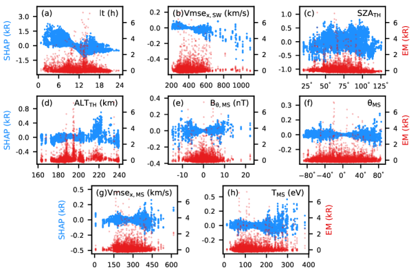
Figure 10: Distribution of SHAP values (blue) vs measurements of the important input features from meagnetosheath (MS) and thermosphere (TH) insitu measurements as well as TH remote sensing geometry measurements as identified in Table 3. The distribution of Ly-$\alpha$ enhancement (EM) corresponding to each measurement is also shown (red).

References

- Acuña et al. (2001) Acuña, M. H., Connerney, J. E. P., Wasilewski, P., et al. 2001, Journal of Geophysical Research: Planets, 106, 23403, doi: https://doi.org/10.1029/2000JE001404
- Atri et al. (2022) Atri, D., Dhuri, D. B., Simoni, M., & Sreenivasan, K. R. 2022, The European Physical Journal D, 76, 235
- Chaffin et al. (2022) Chaffin, M. S., Fowler, C. M., Deighan, J., et al. 2022, Geophysical Research Letters, 49, e2022GL099881, doi: https://doi.org/10.1029/2022GL099881
- Connerney et al. (2015) Connerney, J. E. P., Espley, J., Lawton, P., et al. 2015, Space Science Reviews, 195, 257, doi: 10.1007/s11214-015-0169-4
- Deighan et al. (2018) Deighan, J., Jain, S. K., Chaffin, M. S., et al. 2018, Nature Astronomy, 2, 802, doi: 10.1038/s41550-018-0538-5
- Gao et al. (2021) Gao, J. W., Rong, Z. J., Klinger, L., et al. 2021, Earth and Space Science, 8, e2021EA001860, doi: https://doi.org/10.1029/2021EA001860
- Goodfellow et al. (2016) Goodfellow, I., Bengio, Y., & Courville, A. 2016, Deep Learning (The MIT Press)
- Halekas et al. (2015) Halekas, J. S., Taylor, E. R., Dalton, G., et al. 2015, Space Science Reviews, 195, 125, doi: 10.1007/s11214-013-0029-z
- Halekas et al. (2017a) Halekas, J. S., Ruhunusiri, S., Harada, Y., et al. 2017a, Journal of Geophysical Research: Space Physics, 122, 547, doi: https://doi.org/10.1002/2016JA023167
- Halekas et al. (2017b) Halekas, J. S., Brain, D. A., Luhmann, J. G., et al. 2017b, Journal of Geophysical Research: Space Physics, 122, 11,320, doi: https://doi.org/10.1002/2017JA024772
- Hara et al. (2018) Hara, T., Luhmann, J. G., Leblanc, F., et al. 2018, Journal of Geophysical Research: Space Physics, 123, 8572, doi: https://doi.org/10.1029/2017JA024798
- Hastie et al. (2001) Hastie, T., Tibshirani, R., & Friedman, J. 2001, The Elements of Statistical Learning, Springer Series in Statistics (New York, NY, USA: Springer New York Inc.)
- He et al. (2023) He, F., Fan, K., Hughes, A., et al. 2023, Geophysical Research Letters, 50, e2023GL102723, doi: https://doi.org/10.1029/2023GL102723
- Holsclaw et al. (2021) Holsclaw, G. M., Deighan, J., Almatroushi, H., et al. 2021, Space Science Reviews, 217, 79, doi: 10.1007/s11214-021-00854-3
- Hughes et al. (2019) Hughes, A., Chaffin, M., Mierkiewicz, E., et al. 2019, Journal of Geophysical Research: Space Physics, 124, 10533, doi: https://doi.org/10.1029/2019JA027140
- Hughes (2021) Hughes, A. C. 2021, Doctoral dissertations and master’s theses. 611, Embry-Riddle Aeronautical University, Daytona Beach, FL. https://commons.erau.edu/edt/611
- Jakosky et al. (2015) Jakosky, B. M., Lin, R. P., Grebowsky, J. M., et al. 2015, Space Science Reviews, 195, 3, doi: 10.1007/s11214-015-0139-x
- Lundberg & Lee (2017) Lundberg, S. M., & Lee, S.-I. 2017, in Advances in Neural Information Processing Systems 30, ed. I. Guyon, U. V. Luxburg, S. Bengio, H. Wallach, R. Fergus, S. Vishwanathan, & R. Garnett (Curran Associates, Inc.), 4765–4774. http://papers.nips.cc/paper/7062-a-unified-approach-to-interpreting-model-predictions.pdf
- McClintock et al. (2015) McClintock, W. E., Schneider, N. M., Holsclaw, G. M., et al. 2015, Space Science Reviews, 195, 75, doi: 10.1007/s11214-014-0098-7
- Paszke et al. (2019) Paszke, A., Gross, S., Massa, F., et al. 2019, in Advances in Neural Information Processing Systems, ed. H. Wallach, H. Larochelle, A. Beygelzimer, F. d'Alché-Buc, E. Fox, & R. Garnett, Vol. 32 (Curran Associates, Inc.). https://proceedings.neurips.cc/paper_files/paper/2019/file/bdbca288fee7f92f2bfa9f7012727740-Paper.pdf
- Ritter et al. (2018) Ritter, B., Gérard, J.-C., Hubert, B., Rodriguez, L., & Montmessin, F. 2018, Geophysical Research Letters, 45, 612, doi: https://doi.org/10.1002/2017GL076235
- Selvaraju et al. (2017) Selvaraju, R. R., Cogswell, M., Das, A., et al. 2017, 2017 IEEE International Conference on Computer Vision (ICCV), 1, 618
- Shrikumar et al. (2017) Shrikumar, A., Greenside, P., & Kundaje, A. 2017, in Proceedings of the 34th International Conference on Machine Learning - Volume 70, ICML’17 (JMLR.org), 3145–3153
- Simonyan et al. (2013) Simonyan, K., Vedaldi, A., & Zisserman, A. 2013, CoRR, abs/1312.6034, 1
- Sundararajan et al. (2017) Sundararajan, M., Taly, A., & Yan, Q. 2017, in Proceedings of Machine Learning Research, Vol. 70, Proceedings of the 34th International Conference on Machine Learning, ed. D. Precup & Y. W. Teh (PMLR), 3319–3328. https://proceedings.mlr.press/v70/sundararajan17a.html
- Trotignon et al. (2006) Trotignon, J., Mazelle, C., Bertucci, C., & Acuña, M. 2006, Planetary and Space Science, 54, 357, doi: https://doi.org/10.1016/j.pss.2006.01.003
- Zeiler & Fergus (2014) Zeiler, M., & Fergus, R. 2014, in Lecture Notes in Computer Science (including subseries Lecture Notes in Artificial Intelligence and Lecture Notes in Bioinformatics), Vol. 8689 LNCS, Computer Vision, ECCV 2014 - 13th European Conference, Proceedings, part 1 edn. (Springer Verlag), 818–833, doi: 10.1007/978-3-319-10590-1_53