Angular distribution of the FCNC process $B_{c}\to{D}_{s}^{*}(\to{D}_{s}\pi)\ell^{+}\ell^{-}$

Abstract

In this work, we study the flavor-changing neutral-current process $B_{c}\to{D}_{s}^{*}(\to{D}_{s}\pi)\ell^{+}\ell^{-}$ ($\ell$= $e$, $\mu$, $\tau$). The relevant weak transition form factors are obtained by using the covariant light-front quark model, in which, the main inputs, i.e., the meson wave functions of $B_{c}$ and $D_{s}^{*}$, are adopted as the numerical wave functions from the solution of the Schrödinger equation with the modified Godfrey-Isgur model. With the obtained form factors, we further investigate the relevant branching fractions and their ratios, and some angular observables, i.e., the forward-backward asymmetry $A_{FB}$, the polarization fractions $F_{L(T)}$, and the $CP$-averaged angular coefficients $S_{i}$ and the $CP$ asymmetry coefficients $A_{i}$. We also present our results of the clean angular observables $P_{1,2,3}$ and $P^{\prime}_{4,5,6,8}$, which can reduce the uncertainties from the form factors. Our results show that the corresponding branching fractions of the electron or muon channels can reach up to $10^{-8}$. With more data being accumulated in the LHCb experiment, our results are helpful for exploring this process, and deepen our understanding of the physics around the $b\to{s}\ell^{+}\ell^{-}$ process.

I Introduction

The flavor-changing neutral-current (FCNC) process, like the $b\to{s}\ell^{+}\ell^{-}$ ($\ell$=$e$, $\mu$, $\tau$) we are concerned with has attracted the attention of both theorists and experimentalists, and of course has been widely studied. The FCNC process is forbidden at the tree level, and can only operate through loop diagrams in the Standard Model (SM). At the lowest order, three amplitudes contribute to the decay width, i.e., the photo penguin diagram, the $Z$ penguin diagram, and the $W^{+}W^{-}$ box diagram. In all three diagrams, the virtual $t$ quark plays a dominant role, while the $c$ and $u$ quarks are the secondary contributions. The FCNC process is very sensitive to the new physical effects. This suggests that it can serve as a perfect platform to search directly for new physics (NP) beyond the SM Altmannshofer:2014rta ; Descotes-Genon:2015uva ; SinghChundawat:2022ldm .

The $b\to{s}\ell^{+}\ell^{-}$ in the bottom(-stranged) mesons sector is an attractive experimental topic. The experimental search of the FCNC processes $B\to K^{(*)}\ell^{+}\ell^{-}$ started in 1998 Skwarnicki:1998ph ; CDF:1999uew ; BaBar:2000jlq . The first observation of $B\to{K}\ell^{+}\ell^{-}$ was made by the Belle collaboration in 2001 with a statistical significance of $5.3$ Belle:2001oey . From 2001 to now, the $B\to{K}^{(*)}\ell^{+}\ell^{-}$ with $\ell^{+}\ell^{-}$ being either an $e^{+}e^{-}$ or $\mu^{+}\mu^{-}$ pair has been observed or measured by the Belle Belle:2001oey ; Belle:2003ivt ; Belle:2009zue ; Belle:2016fev ; BELLE:2019xld ; Belle:2019oag , the $BABAR$ BaBar:2003szi ; BaBar:2008jdv ; BaBar:2012mrf , the CDF CDF:2011buy , the CMS CMS:2015bcy , and the LHCb collaborations LHCb:2012juf ; LHCb:2013ghj ; LHCb:2014vgu ; LHCb:2016ykl ; LHCb:2017avl ; LHCb:2021trn . In particular, the LHCb collaboration measured the form-factor-independent observable $P_{5}^{\prime}$ LHCb:2013ghj , and found a $2.5$ standard deviation ($\sigma$) discrepancy to the SM prediction Egede:2008uy after integrating over $1.0<q^{2}<6.0$ $\text{GeV}^{2}$. In addition, the LHCb collaboration recently reported the most precise measurement of the ratio of branching fractions for $B^{+}\to{K}^{+}\mu^{+}\mu^{-}$ and $B^{+}\to{K}^{+}e^{+}e^{-}$ decays in $1.1<q^{2}<6.0~{}\text{GeV}^{2}$ as $R^{{\mu}{e}}_{K}=0.846^{+0.044}_{-0.041}$ LHCb:2021trn , indicating a $3.1$$\sigma$ discrepancy with the SM prediction Descotes-Genon:2015uva ; Bordone:2016gaq , and providing evidence for the violation of lepton flavor universality (LFU). For the $B_{s}$ decays, there have been some experiments, such as the CDF CDF:2001yrm ; CDF:2008zhr and the $\mathrm{D}\O$ experiments D0:2006pmq , to search for the $B_{s}\to\phi\ell^{+}\ell^{-}$ mode. In 2011, the $B_{s}\to\phi\mu^{+}\mu^{-}$ mode was first observed in the CDF experiment CDF:2011grz , and then measured by the CDF CDF:2011buy and the LHCb collaborations LHCb:2013tgx ; LHCb:2015wdu ; LHCb:2021zwz . The electron mode is still missing in the experiment. Moreover, in Ref. LHCb:2021zwz the LHCb collaboration also reported their measurement of the $B_{s}\to{f}_{2}^{\prime}(1525)\mu^{+}\mu^{-}$ process. Compared to the dielectronic and dimuonic modes, the ditauic mode is less studied. There is a Belle experiment, which focused on the $B^{0}\to{K}^{*0}\tau^{+}\tau^{-}$ process, and determined the upper limit of the branching fraction $\mathcal{B}(B^{0}\to K^{*0}\tau^{+}\tau^{-})<3.1\times 10^{-3}$ at $90\%$ confidence level Belle:2021ecr .

The FCNC decay of bottom(-stranged) mesons has also been studied by various theoretical approaches, such as the lattice QCD (LQCD) Bouchard:2013eph ; Horgan:2013hoa ; Bailey:2015dka , the light-cone sum rule Ball:2004rg ; Ball:2004ye ; Wu:2006rd ; Bartsch:2009qp ; Bharucha:2015bzk ; Cheng:2017bzz ; Gao:2019lta ; Wang:2015vgv ; Wang:2017jow ; Lu:2018cfc ; Gao:2021sav ; Cui:2022zwm ; Cui:2023bzr , the QCD factorization Bobeth:2008ij , the perturbative QCD (pQCD) Li:2009tx ; Wang:2007an ; Li:2009rc ; Wang:2012ab ; Wang:2013ix ; Xiao:2013lia and its combination with LQCD data Jin:2020jtu ; Jin:2020qfp , as well as various quark models Deandrea:2001qs ; Geng:2003su ; Chen:2010aq ; Li:2010ra ; Dubnicka:2016nyy ; Soni:2020bvu ; Issadykov:2022imz , and so on Lu:2011jm ; Ahmady:2019hag ; Rajeev:2020aut . On the other hand, in order to understand the discrepancy of the value of $R$ with the SM prediction, the effects beyond the SM are considered. Following this line of thought, the extensions of the SM via the extended Higgs-boson Li:2018rax ; Barman:2018jhz ; DelleRose:2019ukt ; Ordell:2019zws ; Marzo:2019ldg ; Iguro:2018qzf ; Iguro:2023jju , supersymmetry Aslam:2009cv ; Trifinopoulos:2019lyo , and extra dimensions Shaw:2019fin have been used. At the same time, some NP models with an additional heavy neutral boson Altmannshofer:2014cfa ; Bhattacharya:2014wla ; Crivellin:2015lwa ; Celis:2015ara ; Falkowski:2015zwa ; Bhattacharya:2016mcc ; Chiang:2017hlj ; King:2017anf ; Falkowski:2018dsl ; Allanach:2019mfl ; Dwivedi:2019uqd ; Capdevila:2020rrl ; Sheng:2021tom or leptoquarks Hiller:2014yaa ; Gripaios:2014tna ; deMedeirosVarzielas:2015yxm ; Becirevic:2017jtw ; DiLuzio:2017vat ; Becirevic:2018afm ; Angelescu:2018tyl ; Cornella:2019hct ; Popov:2019tyc ; DaRold:2019fiw ; Hati:2019ufv ; Datta:2019bzu ; Balaji:2019kwe ; Crivellin:2019dwb ; Saad:2020ihm ; Babu:2020hun ; Iguro:2021kdw were also considered.

Although great progress has been made both experimentally and theoretically in the rare semileptonic decays of bottom(-strange) mesons in recent decades, those of bottom-charmed mesons have been less studied. Compared to the $B_{(s)}$ mesons, the $B_{c}$ meson is difficult to produce at the Belle experiment because the $B_{c}\bar{B}_{c}$ is close to 12.5 GeV, which is far from the energy region of $\Upsilon(4S)$. Moreover, according to $f_{c}/f_{u}=(7.5\pm 1.8)\times 10^{-3}$ measured by the LHCb collaboration LHCb:2019tea , the $B_{c}$ meson is also underproductivity in the $pp$ experiment. Here, the $f_{c}$ and $f_{u}$ are the fragmentation fractions of $B_{c}$ and $B$ meson, respectively, in $pp$ collisions. As a result, the $B_{c}$ meson decay has received less experimental attention in the past. Recently, the LHCb collaboration reported the result of the $B_{c}^{+}\to{D}_{s}^{+}\mu^{+}\mu^{-}$ process LHCb:2023lyb . Using the $pp$ collision data collected by the LHCb experiment at the center-of-mass energies of 7, 8, and 13 TeV, corresponding to a total integrated luminosity of 9 $\text{fb}^{-1}$, the LHCb collaboration did not observe significant signals in the nonresonant $\mu^{+}\mu^{-}$ modes, but set an upper limit as $f_{c}/f_{u}\times\mathcal{B}(B_{c}^{+}\to{D}_{s}^{+}\mu^{+}\mu^{-})<9.6\times 10^{-8}$ at the $95\%$ confidence level. Moreover, considering that the $B_{c}\to D_{s}^{(*)}\ell^{+}\ell^{-}$ channels have similar amounts of branching fractions Wang:2014yia , and the $D_{s}^{*}$ needs to be reconstructed by the $D_{s}$ meson in the experiment, the measurement of $B_{c}\to D_{s}^{*}\ell^{+}\ell^{-}$ will be more difficult. This indicates that the search for rare semileptonic decays of $B_{c}$ is difficult for the present experiment. However, with the high-luminosity upgrade of the Large Hadron Collider (LHC), this situation is likely to improve. In any case, with the accumulation of data in the experiment, we expect the LHCb experiment to search for these rare semileptonic decays of the $B_{c}$ meson.

In the theoretical sector, the rare semileptonic decays of $B_{c}$ have been studied by the light-front quark model (LFQM) Geng:2001vy , the pQCD Wang:2014yia , the QCD sum rule Kiselev:2002vz ; Azizi:2008vv , the constituent quark model (CQM) Geng:2001vy , et al. The branching fractions of $B_{c}\to{D_{s}^{*}}\ell^{+}\ell^{-}$ with $\ell=e$ or $\mu$ are predicted to be approximately $10^{-7}$. In Refs. Dutta:2019wxo ; Mohapatra:2021ynn ; Zaki:2023mcw , the $B_{c}\to{D_{s}^{*}}\mu^{+}\mu^{-}$ process was been studied within the SM and beyond. In this work, we also focus on the $B_{c}\to{D}_{s}^{*}\ell^{+}\ell^{-}$ process, where the necessary form factors are calculated via the covariant LFQM approach. To provide more physical observables, we present the angular distribution of the quasi-four-body process $B_{c}\to{D_{s}^{*}}(\to{D_{s}}\pi)\ell^{+}\ell^{-}$.

The applications of the standard and(or) covariant LFQM have proved successful in the study of the meson Jaus:1989au ; Jaus:1996np ; Cheng:1996if ; Cheng:1997au ; Jaus:1999zv ; Cheng:2003sm ; Chua:2003ac ; Cheng:2004yj ; Wang:2007sxa ; Wang:2008ci ; Shen:2008zzb ; Wang:2008xt ; Wang:2009mi ; Cheng:2009ms ; Chen:2009qk ; Choi:2010zb ; Choi:2010be ; Li:2010bb ; Ke:2011mu ; Verma:2011yw ; Ke:2013yka ; Xu:2014mqa ; Shi:2016gqt ; Cheng:2017pcq ; Chen:2017vgi ; Kang:2018jzg ; Chang:2018zjq ; Chang:2019mmh ; Chang:2019xtj ; Chang:2019obq ; Chang:2020xvu ; Chang:2020wvs ; Chen:2021ywv ; Choi:2021mni ; Choi:2021qza ; Arifi:2022qnd ; Zhang:2023ypl ; Shi:2023qnw ; Hazra:2023zno ; Zhang:2020dla and baryon weak decays Ke:2007tg ; Ke:2012wa ; Wang:2017mqp ; Ke:2017eqo ; Zhu:2018jet ; Zhao:2018zcb ; Zhao:2018mrg ; Xing:2018lre ; Chua:2018lfa ; Ke:2019smy ; Chua:2019yqh ; Ke:2019lcf ; Hu:2020mxk ; Geng:2020fng ; Hsiao:2020gtc ; Geng:2021nkl ; Li:2021qod ; Ke:2021pxk ; Hsiao:2021mlp ; Li:2021kfb ; Li:2022nim ; Geng:2022xpn ; Wang:2022ias ; Zhao:2022vfr ; Li:2022hcn ; Lu:2023rmq ; Zhao:2023yuk ; Liu:2023zvh . The $B_{c}\to{D}_{s}^{*}$ weak transition form factors deduced by (axial)-vector currents have been calculated in Ref. Zhang:2023ypl with the covariant LFQM. Probably in the series of papers Cheng:2003sm ; Chua:2003ac ; Wang:2007sxa ; Wang:2008ci ; Shen:2008zzb ; Wang:2008xt ; Wang:2009mi ; Chen:2009qk ; Cheng:2009ms ; Choi:2010zb ; Li:2010bb ; Verma:2011yw ; Ke:2013yka ; Xu:2014mqa ; Shi:2016gqt ; Chang:2018zjq ; Chang:2019xtj ; Chang:2019obq ; Chang:2019mmh ; Chang:2020xvu ; Chang:2020wvs ; Chen:2021ywv ; Choi:2021mni ; Choi:2021qza ; Arifi:2022qnd ; Shi:2023qnw ; Ke:2007tg ; Ke:2012wa ; Ke:2017eqo ; Wang:2017mqp ; Zhu:2018jet ; Zhao:2018zcb ; Xing:2018lre ; Chua:2018lfa ; Zhao:2018mrg ; Chua:2019yqh ; Ke:2019lcf ; Ke:2019smy ; Hu:2020mxk ; Geng:2020fng ; Hsiao:2020gtc ; Hsiao:2021mlp ; Geng:2021nkl ; Ke:2021pxk ; Zhao:2022vfr ; Geng:2022xpn ; Wang:2022ias ; Liu:2023zvh ; Lu:2023rmq ; Zhao:2023yuk , the hadron wave function was taken as a Gaussian-like form with phenomenal parameter $\beta$, which represents the hadron structure. To fix the phenomenal parameter, the corresponding decay constant was used. However, as we all know, the decay constant is only associated with the zero-point wave function. This indicates that the oversimplified Gaussian-form wave function is not able to depict the behavior far away from the zero point. For this object, we propose to directly adopt the numerical spatial wave function by solving the Schrödinger equation with the modified Godfrey-Isgur (GI) model. By fitting the mass spectrum of the observed heavy flavor mesons, the parameters of the potential model can be fixed. This strategy avoids the $\beta$ dependence, and can also reduce the corresponding uncertainty. We note that in Ref. Faustov:2022ybm , the authors used a relativistic quark model based on the quasipotential approach in QCD to study the semileptonic decay of bottom mesons. In their approach, the numerical wave functions of the mesons are obtained, thus avoiding the corresponding uncertainty.

This paper is organized as follows. After the Introduction, we illustrate the angular distributions of the quasi-four-body decays $B_{c}\to{D}_{s}^{*}(\to{D}_{s}\pi)\ell^{+}\ell^{-}$ ($\ell$= $e$, $\mu$, $\tau$) in Sec. II. In Sec. III, we introduce the covariant LFQM and derive the formula of the weak transition form factors. Then in Sec. IV, the numerical results, including the from factors of $B_{c}\to{D}_{s}^{*}$ and physical observables of $B_{c}\to{D}_{s}^{*}(\to{D}_{s}\pi)\ell^{+}\ell^{-}$ processes, are presented. Finally, this paper ends with a short summary.

II The angular distribution of $B_{c}\to{D}_{s}^{*}(\to{D}_{s}\pi)\ell^{+}\ell^{-}$

II.1 The effective Hamiltonian for $b\to{s}\ell^{+}\ell^{-}$

The effective Hamiltonian associated with $b\to{s}\ell^{+}\ell^{-}$ is Buchalla:1995vs

$$\begin{split}\mathcal{H}{\!}=&{\!}-{\!}\frac{4G_{F}}{\sqrt{2}}\Big{\{}V_{tb}V_{ts}^{*}\bigg{[}{C}_{1}(\mu)\mathcal{O}_{1}^{c}(\mu){\!}+{\!}{C}_{2}(\mu)\mathcal{O}_{2}^{c}(\mu){\!}+{\!}\sum_{i=3}^{10}{C}_{i}(\mu)\mathcal{O}_{i}(\mu)\bigg{]}\\ &{\!}+{\!}V_{ub}V_{us}^{*}\big{[}{C}_{1}(\mu)(\mathcal{O}_{1}^{c}(\mu){\!}-{\!}\mathcal{O}_{1}^{u}(\mu)){\!}+{\!}{C}_{2}(\mu)(\mathcal{O}_{2}^{c}(\mu){\!}-{\!}\mathcal{O}_{2}^{u}(\mu))\big{]}\Big{\}},\end{split}$$ (2.1)

where $V_{ij}$ are the Cabibbo-Kobayashi-Maskawa (CKM) matrix elements and $G_{F}=1.16637\times 10^{-5}~{}\text{GeV}^{-2}$ ParticleDataGroup:2022pth is the Fermi constant. Also, the ${C}_{i}(\mu)$ are Wilson coefficients and the $\mathcal{O}_{i}(\mu)$ are four fermion operators. They all depend on the QCD renormalization scale $\mu$. More specifically, the $\mathcal{O}_{1,2}^{c,u}$ are current-current operations, the $\mathcal{O}_{3-6}$ are QCD penguin operators, the $\mathcal{O}_{7,8}$ are electromagnetic and chromomagnetic penguin operators, and the $\mathcal{O}_{9,10}$ are semileptonic operators, respectively.

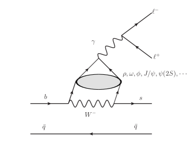
Figure 1: The contributions of the intermediate vector states $(\rho,\omega,\phi.J/\psi,\psi(2S),\dots)$ to the $b\to{s}\ell^{+}\ell^{-}$ process resulting from the current-current operators $\mathcal{O}_{1,2}^{c,u}$.

Apart from the $\gamma$ and $Z$ penguin diagrams, and the $W^{+}W^{-}$ box diagram, the long distance contribution, via the intermediate vector states $(\rho,\omega,\phi.J/\psi,\psi(2S),\dots)$ (see Fig. 1) also shows an unignorable influence. By adding the factorable quark-loop contributions from $\mathcal{O}_{1-6,8}$ to the effective Wilson coefficients ${C}_{7,9}^{\text{eff}}$, the effective Hamiltonian in Eq. (2.1) can be simplified. In the calculation, we have adopted the following effective Hamiltonian, i.e.,

$$\begin{split}\mathcal{H}^{\text{eff}}(b\to{s}\ell^{+}\ell^{-})=&-\frac{4G_{F}}{\sqrt{2}}V_{tb}V_{ts}^{*}\frac{\alpha_{e}}{4\pi}\bigg{\{}\bar{s}\big{[}{C}_{9}^{\text{eff}}(q^{2},\mu)\gamma^{\mu}P_{L}\\ &-\frac{2m_{b}}{q^{2}}{C}_{7}^{\text{eff}}(\mu)i\sigma^{\mu\nu}q_{\nu}P_{R}\big{]}b(\bar{\ell}\gamma_{\mu}\ell)\\ &+{C}_{10}(\mu)(\bar{s}\gamma^{\mu}P_{L}b)(\bar{\ell}\gamma_{\mu}\gamma_{5}\ell)\bigg{\}},\end{split}$$ (2.2)

where $P_{L(R)}=(1\mp\gamma_{5})/2$, $\sigma^{\mu\nu}=i(\gamma^{\mu}\gamma^{\nu}-\gamma^{\nu}\gamma^{\mu})/2$, and the electromagnetic coupling constant $\alpha_{e}=1/137$. The $\mathcal{C}_{7}^{\text{eff}}$ and $\mathcal{C}_{9}^{\text{10}}$ are the effective Wilson coefficients, defined as Chen:2001zc

$$\begin{split}{C}_{7}^{\text{eff}}(\mu)=&{C}_{7}(\mu)+{C}^{\prime}_{b\to s\gamma}(\mu),\\ {C}_{9}^{\text{eff}}(q^{2},\mu)=&{C}_{9}(\mu)+Y_{\text{pert}}(q^{2},\mu)+Y_{\text{res}}(q^{2},\mu),\end{split}$$ (2.3)

where the term ${C}^{\prime}_{b\to{s}{\gamma}}$ is the absorptive part of the $b\to{s}{c}{\bar{c}}\to{s}{\gamma}$ rescattering Asatrian:1996as ; Chen:2001zc ; Aslam:2008hp ; Aslam:2009cv ; Wang:2012ab ; Soni:2020bvu ; Jin:2020jtu ; Jin:2020qfp :

$$\begin{split}{C}^{\prime}_{b\to s\gamma}(\mu)=&i\alpha_{s}\Big{\{}\frac{2}{9}\eta^{\frac{14}{23}}\Big{[}\frac{x_{t}(x_{t}^{2}-5x_{t}-2)}{8(x_{t}-1)^{3}}+\frac{3x_{t}^{2}\ln x_{t}}{4(x_{t}-1)^{4}}-0.1687\Big{]}\\ &-0.03\mathcal{C}_{2}(\mu)\Big{\}}\end{split}$$ (2.4)

with $x_{t}=m_{t}^{2}/m_{W}^{2}$, $\eta=\alpha_{s}(m_{W})/\alpha_{s}(\mu)$, and $\alpha_{s}$ being adopted as $\alpha_{s}(m_{b})=0.217$ in our calculation. The short-distance contributions from the soft-gluon emission and the one-loop contributions of the four fermion operators $\mathcal{O}_{1}-\mathcal{O}_{6}$, and the long-distance contributions from the intermediate vector meson states are also taken into account, and have been included in the $Y_{\text{pert}}$ and $Y_{\text{res}}$ terms, respectively. The $Y_{\text{pert}}$ can be written as Buras:1994dj

$$\begin{split}Y_{\text{pert}}(\hat{s},\mu)=&0.124\omega(\hat{s})+g(\hat{m}_{c},\hat{s}){C}(\mu)\\ &+\lambda_{\mu}\Big{[}g(\hat{m}_{c},\hat{s})-g(0,\hat{s})\Big{]}(3{C}_{1}(\mu)+{C}_{2}(\mu))\\ &-\frac{1}{2}g(0,\hat{s})({C}_{3}(\mu)+3{C}_{4}(\mu))\\ &-\frac{1}{2}g(1,\hat{s})(4{C}_{3}(\mu)+4{C}_{4}(\mu)+3{C}_{5}(\mu)+{C}_{6}(\mu))\\ &+\frac{2}{9}(3{C}_{3}(\mu)+{C}_{4}(\mu)+3{C}_{5}(\mu)+{C}_{6}(\mu)),\end{split}$$ (2.5)

where $\hat{s}=q^{2}/m_{b}^{2}$ and $\hat{m}_{c}=m_{c}/m_{b}$ with $m_{b}=4.8~{}\text{GeV}$ and $m_{c}=1.6~{}\text{GeV}$, and ${C}(\mu)=3{C}_{1}(\mu)+{C}_{2}(\mu)+3{C}_{3}(\mu)+{C}_{4}(\mu)+3{C}_{5}(\mu)+{C}_{6}(\mu)$. At the next leading order, the Wilson coefficients at the QCD renormalization scale $\mu=m_{b}$ are chosen as $C_{1}=-0.175$, $C_{2}=1.076$, $C_{3}=1.258\%$, $C_{4}=-3.279\%$, $C_{5}=1.112\%$, $C_{6}=-3.634\%$, $C_{7}=-0.302$, $C_{8}=-0.148$, $C_{9}=4.232$, and $C_{10}=-4.410$ Buchalla:1995vs .

In the Wolfenstein representation, the $\lambda_{u}=V_{ub}V_{us}^{*}/(V_{tb}V_{ts}^{*})$ can be expressed as

$$\lambda_{u}\approx-\lambda^{2}(\rho-i\eta),$$ (2.6)

approximately, which is a small value suppressed by $\lambda^{2}$ with $\lambda=0.22500\pm 0.00067$ ParticleDataGroup:2022pth .

In addition, the term $\Omega(\hat{s})$ is the one-gluon correction to the matrix element of the operator $\mathcal{O}_{9}$, represented as Buras:1994dj ; Jin:2020jtu

$$\begin{split}\omega(\hat{s})=&-\frac{2}{9}\pi^{2}+\frac{4}{3}\int_{0}^{\hat{s}}\frac{\ln{1-u}}{u}du-\frac{2}{3}\ln{(\hat{s})}\ln{(1-\hat{s})}\\ &-\frac{5+4\hat{s}}{3(1+2\hat{s})}\ln{(1-\hat{s})}-\frac{2\hat{s}(1+\hat{s})(1-2\hat{s})}{3(1-\hat{s})^{2}(1+2\hat{s})}\ln{(\hat{s})}\\ &+\frac{5+9\hat{s}-6\hat{s}^{2}}{6(1-\hat{s})(1+2\hat{s})},\end{split}$$ (2.7)

and the $g$ terms Buras:1994dj ; Aslam:2008hp ; Aslam:2009cv ; Wang:2012ab ; Soni:2020bvu :

$$\begin{split}g(z,\hat{s})=&-\frac{8}{9}\ln{z}+\frac{8}{27}+\frac{4}{9}x-\frac{2}{9}(2+x)\sqrt{|1-x|}\\ &\times\begin{array}[]{ll}\ln|\frac{1+\sqrt{1-x}}{1-\sqrt{1-x}}|-i\pi&\text{for}\ x\equiv 4z^{2}/\hat{s}<1\\ 2\arctan{\frac{1}{\sqrt{x-1}}}&\text{for}\ x\equiv 4z^{2}/\hat{s}>1\end{array},\\ g(0,\hat{s})=&\frac{8}{27}-\frac{8}{9}\ln{\frac{m_{b}}{\mu}}-\frac{4}{9}\ln{\hat{s}}+\frac{4}{9}i\pi,\end{split}$$ (2.8)

come from the one-loop contributions of the $\mathcal{O}_{1-6}$.

The $Y_{\text{res}}$ term, which describes the long-distance contributions associated with the intermediate light vector mesons (such as $\rho$, $\omega$, and $\phi$) and vector charmonium states [such as $J/\psi$, $\psi(2S)$, etc.] (see the Fig. 1), is adopted as Jin:2020jtu

$$\begin{split}Y_{\text{res}}(q^{2},\mu)=&-\frac{3\pi}{\alpha_{e}^{2}}\bigg{[}{C}(\mu)\sum_{V_{i}=J/\psi,\psi(2S),\dots}\frac{m_{V_{i}}\mathcal{B}(V_{i}\to\ell^{+}\ell^{-})\Gamma_{V_{i}}}{q^{2}-m_{V_{i}}^{2}+im_{V_{i}}\Gamma_{V_{i}}}\\ &-\lambda_{u}g(0,\hat{s})(3{C}_{1}(\mu)+{C}_{2}(\mu))\\ &\times\sum_{V_{j}=\rho,\omega,\phi}\frac{m_{V_{j}}\mathcal{B}(V_{j}\to\ell^{+}\ell^{-})\Gamma_{V_{j}}}{q^{2}-m_{V_{j}}^{2}+im_{V_{j}}\Gamma_{V_{j}}}\bigg{]},\end{split}$$ (2.9)

where $m_{V_{i}}$ and $\Gamma_{V_{i}}$ are the mass and total width of the intermediate vector meson $V_{i}$ respectively, and the $\Gamma(V_{i}\to\ell^{+}\ell^{-})$ is the corresponding dilepton width. These input values are collected in Table 1. In addition, the nonvanished branching fraction for the $\tau$ channel, i.e., $\mathcal{B}(\psi(2S)\to\tau^{+}\tau^{-})=3.1\times 10^{-3}$ ParticleDataGroup:2022pth , is also used.

For the $J/\psi$ and $\psi(2S)$ states, the small widths and the large dilepton width will have a large influence on the decay width. However, the narrow widths are also used to reject them in the experimental analysis. One the other hand, for those above the $D\bar{D}$ threshold, such as $\psi(3770)$, $\psi(4040)$ and $\psi(4160)$, the board widths and mutual overlap make things difficult. Also, for the charmless vector mesons ($\rho$, $\omega$ and $\phi$), their contributions are suppressed by the $\lambda_{u}$ factor.

Table 1: The masses, total widths and dilepton widths of the intermediate vector mesons used in Eq. (2.9). These values are quoted from the PDG ParticleDataGroup:2022pth .

$V_{i}$	$m_{V_{i}}$ (GeV)	$\Gamma_{V_{i}}$ (MeV)	$\mathcal{B}(V_{i}\to\ell^{+}\ell^{-})$
			where $\ell=e,\mu$
$\rho$	$0.775$	$149$	$4.635\times 10^{-5}$
$\omega$	$0.783$	$8.68$	$7.380\times 10^{-5}$
$\phi$	$1.019$	$4.249$	$2.915\times 10^{-4}$
$J/\psi$	$3.097$	$0.093$	$5.966\times 10^{-2}$
$\psi(2S)$	$3.686$	$0.294$	$7.965\times 10^{-3}$
$\psi(3770)$	$3.774$	$27.2$	$9.6\times 10^{-6}$
$\psi(4040)$	$4.039$	$80$	$1.07\times 10^{-5}$
$\psi(4160)$	$4.191$	$70$	$6.9\times 10^{-6}$

II.2 The angular distributions and physical observables in the $B_{c}\to D_{s}^{*}(\to D_{s}\pi)\ell^{+}\ell^{-}$ decay

In this subsection, we will drive the formula of the quasi-four-body decay $B_{c}\to D_{s}^{*}(\to D_{s}\pi)\ell^{+}\ell^{-}$. The differential decay width of this process is

$$d\Gamma=\frac{|\mathcal{M}|^{2}}{2m_{B_{c}}}d\Phi_{4}(p;k_{1},k_{2},q_{1},q_{2}),$$ (2.10)

where $p$ is the four momentum of the initial $B_{c}$ meson, $k_{1}(k_{2})$ and $q_{1}(q_{2})$ are the momenta of the mesons $D_{s}(\pi)$ and the lepton $\ell^{-}(\ell^{+})$, respectively, and $d\Phi_{4}$ is the four-body phase space. Taking into account the width of the $D_{s}^{*}$ meson, but treating it as narrow ($\Gamma_{D_{s}^{*}}\ll m_{D_{s}^{*}}$), the width can be obtained by doing the integration as

$$\begin{split}\int d\Phi_{4}\frac{|\mathcal{M}|^{2}}{2m_{B_{c}}}\stackrel{{\scriptstyle\Gamma_{D_{s}^{*}}\ll m_{D_{s}^{*}}}}{{\longrightarrow}}&\frac{1}{2^{15}\pi^{5}m_{B_{c}}m_{D_{s}^{*}}\Gamma_{D_{s}^{*}}}\int dq^{2}d\cos\theta d\cos\theta_{\ell}d\phi\\ &\times\frac{\sqrt{\lambda(k^{2},k_{1}^{2},k_{2}^{2})}}{k^{2}}\frac{\sqrt{\lambda(q^{2},q_{1}^{2},q_{2}^{2})}}{q^{2}}\\ &\times\frac{\sqrt{\lambda(p^{2},k^{2},q^{2})}}{p^{\prime 2}}(k^{2}-m_{D_{s}^{*}}^{2})^{2}|\mathcal{M}|^{2}\Big{|}_{k^{2}=m_{D_{s}^{*}}^{2}}\end{split}$$ (2.11)

with $\lambda(x,y,z)=x^{2}+y^{2}+z^{2}-2(xy+xz+yz)$.

The invariant amplitude $\mathcal{M}$ can be calculated from

$$\begin{split}\mathcal{M}(s_{\ell^{+}},s_{\ell^{-}})=&\big{\langle}{D_{s}\pi;\ell^{+}(s_{\ell^{+}})\ell^{-}(s_{\ell^{-}})}{|}{\mathcal{H}^{\text{eff}}}{|}{B_{c}}\big{\rangle}\\ =&\sum_{s_{V}}\frac{i}{k^{2}-m_{D_{s}^{*}}^{2}}\mathcal{M}_{D_{s}^{*}\to{D_{s}\pi}}(s_{V})\big{\langle}{D_{s}^{*}(s_{V})}{\ell^{+}(s_{\ell^{+}})\ell^{-}(s_{\ell^{-}})}{|}\mathcal{H}^{\text{eff}}{|}B_{c}\big{\rangle}\\ =&\sum_{s_{V}}\frac{iN}{2(k^{2}-m_{D_{s}^{*}}^{2})}\mathcal{M}_{D_{s}^{*}\to{D_{s}\pi}}(s_{V})\bigg{\{}{C}_{9}^{\text{eff}}H^{V-A}(s_{V},t)L^{V}(s_{\ell^{+}},s_{\ell^{-}},t)-\frac{2m_{b}}{q^{2}}{C}_{7}^{\text{eff}}H^{T+T\text{5}}(s_{V},t)L^{V}(s_{\ell^{+}},s_{\ell^{-}},t)\\ &+{C}_{10}H^{V-A}(s_{V},t)L^{A}(s_{\ell^{+}},s_{\ell^{-}},t)-\sum_{\lambda=\pm 1,0}\bigg{[}{C}_{9}^{\text{eff}}H^{V-A}(s_{V},\lambda)L^{V}(s_{\ell^{+}},s_{\ell^{-}},\lambda)\\ &-\frac{2m_{b}}{q^{2}}{C}_{7}^{\text{eff}}H^{T+T\text{5}}(s_{V},\lambda)L^{V}(s_{\ell^{+}},s_{\ell^{-}},\lambda)+{C}_{10}H^{V-A}(s_{V},\lambda)L^{A}(s_{\ell^{+}},s_{\ell^{-}},\lambda)\bigg{]}\bigg{\}},\end{split}$$ (2.12)

where $N=\frac{4G_{F}}{\sqrt{2}}V_{tb}V_{ts}^{*}\frac{\alpha_{e}}{4\pi}$, and the factor $1/2$ comes from the $P_{L(R)}$ in the effective Hamiltonian in Eq. (2.2).

For the amplitude $\mathcal{M}_{D_{s}^{*}\to D_{s}\pi}$, it can be evaluated by the effective Lagrangian approach. The concerned effective Lagrangian is

$$\mathcal{L}=g_{D_{s}^{*}D_{s}\pi}D_{s}^{\dagger}D_{s\mu}^{*}\partial^{\mu}\pi,$$ (2.13)

where $g_{D_{s}^{*}D_{s}\pi}$ is the corresponding coupling constant. So we have the decay width of $D_{s}^{*}\to D_{s}\pi$ as

$$\Gamma_{D_{s}^{*}}\times\mathcal{B}(D_{s}^{*}\to D_{s}\pi)=\frac{g_{D_{s}^{*}D_{s}\pi}^{2}}{48\pi}m_{D_{s}^{*}}\beta^{3}$$ (2.14)

with $\beta=\sqrt{\lambda(m_{D_{s}^{*}}^{2},m_{D_{s}}^{2},m_{\pi}^{2})}/m_{D_{s}^{*}}^{2}$. Obviously, the coupling constant $g_{D_{s}^{*}D_{s}\pi}$ can be canceled between the vertex factor and the decay width.

Finally, with the effective Hamiltonian in Eq. (2.2), we can calculate the quasi-four-body decay $B_{c}^{-}\to D_{s}^{*-}(\to D_{s}^{-}\pi^{0})\ell^{+}\ell^{-}$. As deduced in Ref. Altmannshofer:2008dz , the corresponding angular distributions can be simplified as

$$\frac{d^{4}\Gamma}{dq^{2}d\cos\theta d\cos\theta_{\ell}d\phi}=\frac{9}{32\pi}\sum_{i}I_{i}(q^{2})f_{i}(\theta,\theta_{\ell},\phi),$$ (2.15)

where the explicit expressions of $I_{i}(q^{2})$ and $f_{i}(\theta,\theta_{\ell},\phi)$ are shown in Table 2. Compared to Ref. Altmannshofer:2008dz , the term $I_{6c}$ is neglected since it depends on the scalar operator. As shown in Fig. 2, the $\theta$ is the angle between the $-\hat{z}$ direction and pion-emitted direction in the rest frame of the $D_{s}^{*}$ meson, the $\theta_{\ell}$ is the angle made by the $\ell^{-}$ with the $+\hat{z}$ direction in the $\ell^{+}\ell^{-}$ center of mass system, and the $\phi$ is the angle between the decay planes, i.e., the $D_{s}^{*}\to D_{s}\pi$ plane and the $\text{virtual~{}boson}\to\ell^{+}\ell^{-}$ plane.

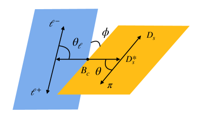
Figure 2: Kinematics of the quasi-four-body decay $B_{c}\to D_{s}^{*}(\to D_{s}\pi)\ell^{+}\ell^{-}$.

Table 2: The explicit expressions of the angular coefficients $I_{i}$ and $f_{i}$ Altmannshofer:2008dz ; Jin:2020jtu ; Jin:2020qfp in Eq. (2.15), where $\hat{m}_{\ell}^{2}=m_{\ell}^{2}/q^{2}$ and $\beta_{\ell}=\sqrt{1-4\hat{m}_{\ell}^{2}}$.

$i$	$I_{i}(q^{2})$	$f_{i}(\theta,\theta_{\ell},\phi)$
$1s$	$\Big{(}\frac{3}{4}-\hat{m}_{\ell}^{2}\Big{)}\Big{(}|\mathscr{A}_{\|}^{L}|^{2}+|\mathscr{A}_{\bot}^{L}|^{2}+|\mathscr{A}_{\|}^{R}|^{2}+|\mathscr{A}_{\bot}^{R}|^{2}\Big{)}+4\hat{m}_{\ell}^{2}\text{Re}\big{[}\mathscr{A}_{\bot}^{L}\mathscr{A}_{\bot}^{R*}+\mathscr{A}_{\|}^{L}\mathscr{A}_{\|}^{R*}\big{]}$	$\sin^{2}\theta$
$1c$	$|\mathscr{A}_{0}^{L}|^{2}+|\mathscr{A}_{0}^{R}|^{2}+4\hat{m}_{\ell}^{2}\Big{(}|\mathscr{A}_{t}|^{2}+2\text{Re}\big{[}\mathscr{A}_{0}^{L}\mathscr{A}_{0}^{R*}\big{]}\Big{)}$	$\cos^{2}\theta$
$2s$	$\beta_{\ell}^{2}\Big{(}|\mathscr{A}_{\|}^{L}|^{2}+|\mathscr{A}_{\bot}^{L}|^{2}+|\mathscr{A}_{\|}^{R}|^{2}+|\mathscr{A}_{\bot}^{R}|^{2}\Big{)}/4$	$\sin^{2}\theta\cos 2\theta_{\ell}$
$2c$	$-\beta_{\ell}^{2}\Big{(}|\mathscr{A}_{0}^{L}|^{2}+|\mathscr{A}_{0}^{R}|^{2}\Big{)}$	$\cos^{2}\theta\cos 2\theta_{\ell}$
$3$	$\beta_{\ell}^{2}\Big{(}|\mathscr{A}_{\bot}^{L}|^{2}-|\mathscr{A}_{\|}^{L}|^{2}+|\mathscr{A}_{\bot}^{R}|^{2}-|\mathscr{A}_{\|}^{R}|^{2}\Big{)}/2$	$\sin^{2}\theta\sin^{2}\theta_{\ell}\cos 2\phi$
$4$	$\beta_{\ell}^{2}\text{Re}\big{[}\mathscr{A}_{0}^{L}\mathscr{A}_{\|}^{L*}+\mathscr{A}_{0}^{R}\mathscr{A}_{\|}^{R*}\big{]}/\sqrt{2}$	$\sin 2\theta\sin 2\theta_{\ell}\cos\phi$
$5$	$\sqrt{2}\beta_{\ell}\text{Re}\big{[}\mathscr{A}_{0}^{L}\mathscr{A}_{\bot}^{L*}-\mathscr{A}_{0}^{R}\mathscr{A}_{\bot}^{R*}\big{]}$	$\sin 2\theta\sin\theta_{\ell}\cos\phi$
$6s$	$2\beta_{\ell}\text{Re}\big{[}\mathscr{A}_{\|}^{L}\mathscr{A}_{\bot}^{L*}-\mathscr{A}_{\|}^{R}\mathscr{A}_{\bot}^{R*}\big{]}$	$\sin^{2}\theta\cos\theta_{\ell}$
$7$	$\sqrt{2}\beta_{\ell}\text{Im}\big{[}\mathscr{A}_{0}^{L}\mathscr{A}_{\|}^{L*}-\mathscr{A}_{0}^{R}\mathscr{A}_{\|}^{R*}\big{]}$	$\sin 2\theta\sin\theta_{\ell}\sin\phi$
$8$	$\beta_{\ell}^{2}\text{Im}\big{[}\mathscr{A}_{0}^{L}\mathscr{A}_{\bot}^{L*}+\mathscr{A}_{0}^{R}\mathscr{A}_{\bot}^{R*}\big{]}/\sqrt{2}$	$\sin 2\theta\sin 2\theta_{\ell}\sin\phi$
$9$	$\beta_{\ell}^{2}\text{Im}\big{[}\mathscr{A}_{\|}^{L*}\mathscr{A}_{\bot}^{L}+\mathscr{A}_{\|}^{R*}\mathscr{A}_{\bot}^{R}\big{]}$	$\sin^{2}\theta\sin^{2}\theta_{\ell}\sin 2\phi$

The amplitudes $\mathscr{A}_{0,\|,\bot}^{L,R}$ and $\mathscr{A}_{t}$ are the functions of the transferred momentum square $q^{2}$, and the seven independent form factors $V$, $A_{0,1,2}$ and $T_{1,2,3}$, i.e., Altmannshofer:2008dz ; Jin:2020jtu ; Jin:2020qfp

$$\begin{split}\mathscr{A}_{\bot}^{L,R}(q^{2})=&-N_{\ell}\sqrt{2N_{D_{s}^{*}}}\sqrt{\lambda(M^{\prime 2},M^{\prime\prime 2},q^{2})}\bigg{[}\Big{(}{C}_{9}^{\text{eff}}\mp{C}_{10}\Big{)}\frac{V(q^{2})}{M^{\prime}+M^{\prime\prime}}+2\hat{m}_{b}{C}_{7}^{\text{eff}}T_{1}(q^{2})\bigg{]},\\ \mathscr{A}_{\|}^{L,R}(q^{2})=&N_{\ell}\sqrt{2N_{D_{s}^{*}}}\bigg{[}\Big{(}{C}_{9}^{\text{eff}}\mp{C}_{10}\Big{)}(M^{\prime}+M^{\prime\prime})A_{1}(q^{2})+2\hat{m}_{b}{C}_{7}^{\text{eff}}\Big{(}M^{\prime 2}-M^{\prime\prime 2}\Big{)}T_{2}(q^{2})\bigg{]},\\ \mathscr{A}_{0}^{L,R}(q^{2})=&\frac{N_{\ell}\sqrt{N_{D_{s}^{*}}}}{2M^{\prime\prime}\sqrt{q^{2}}}\bigg{\{}\Big{(}{C}_{9}^{\text{eff}}\mp{C}_{10}\Big{)}\bigg{[}(M^{\prime 2}-M^{\prime\prime 2}-q^{2})(M^{\prime}+M^{\prime\prime})A_{1}(q^{2})-\frac{\lambda(M^{\prime 2},M^{\prime\prime 2},q^{2})}{M^{\prime}+M^{\prime\prime}}A_{2}(q^{2})\bigg{]}\\ &+2m_{b}{C}_{7}^{\text{eff}}\bigg{[}(M^{\prime 2}+3M^{\prime\prime 2}-q^{2})T_{2}(q^{2})-\frac{\lambda(M^{\prime 2},M^{\prime\prime 2},q^{2})}{M^{\prime 2}-M^{\prime\prime 2}}T_{3}(q^{2})\bigg{]}\bigg{\}},\\ \mathscr{A}_{t}(q^{2})=&2N_{\ell}\sqrt{N_{D_{s}^{*}}}\sqrt{\frac{\lambda(M^{\prime 2},M^{\prime\prime 2},q^{2})}{q^{2}}}{C}_{10}A_{0}(q^{2}),\end{split}$$ (2.16)

where $M^{\prime}(M^{\prime\prime})$ is the mass of the $B_{c}$ ($D_{s}^{*}$) meson and $\hat{m}_{b}=m_{b}/q^{2}$, and

$$\begin{split}N_{\ell}=&\frac{i\alpha_{e}G_{F}}{4\sqrt{2}\pi}V_{tb}V_{ts}^{*},\\ N_{D_{s}^{*}}=&\frac{8\sqrt{\lambda}q^{2}}{3\times 256\pi^{3}M^{\prime 3}}\sqrt{1-\frac{4m_{\ell}^{2}}{q^{2}}}\mathcal{B}\big{(}D_{s}^{*}\to D_{s}\pi\big{)}.\end{split}$$ (2.17)

For the $CP$-conjugated mode $B_{c}^{+}\to D_{s}^{*+}(\to D_{s}^{+}\pi^{0})\ell^{+}\ell^{-}$, we have

$$\frac{d^{4}\bar{\Gamma}}{q^{2}{d\cos\theta}{d\cos\theta_{\ell}}{d\phi}}=\sum_{i}\frac{9}{32\pi}\bar{I}_{i}(q^{2})f_{i}(\theta,\theta_{\ell},\phi),$$ (2.18)

where $\bar{I}_{i}$ can be obtained by doing the conjugation for the weak phases of the CKM matrix elements in $I_{i}$ in Table 2. In addition, we should also do the following substitutions as

$$\begin{split}I_{1(c,s),2(c,s),3,4,7}\to&\bar{I}_{1(c,s),2(c,s),3,4,7},\\ I_{5,6s,8,9}\to&-\bar{I}_{5,6s,8,9}.\end{split}$$ (2.19)

This is the result of the operations of $\theta_{\ell}\to\theta_{\ell}-\pi$ and $\phi\to-\phi$.

To separate the $CP$-conserving and the $CP$-violating effects, we define the normalized $CP$-averaged angular coefficients $S_{i}$ and the $CP$ asymmetry angular coefficients $A_{i}$ as

$$\begin{split}S_{i}=&\frac{I_{i}+\bar{I}_{i}}{d(\Gamma+\bar{\Gamma})/dq^{2}},\\ A_{i}=&\frac{I_{i}-\bar{I}_{i}}{d(\Gamma+\bar{\Gamma})/dq^{2}},\\ \end{split}$$ (2.20)

respectively. To reduce both the experimental and theoretical uncertainties, the $S_{i}$ and $A_{i}$ have been normalized to the $CP$-averaged differential decay width. The other physical observables, such as the forward-backward asymmetry parameter $A_{FB}$, the $CP$-violation $\mathcal{A}_{CP}$, and the longitudinal (transverse) polarization fractions of $D_{s}^{*}$ meson $F_{L}(F_{T})$, can thus be easily expressed in terms of these normalized angular coefficients. With the above preparations, we continue to study the physical observables.

1. By integrating over the angles in the regions $\theta\in[0,\pi]$, $\theta_{\ell}\in[0,\pi]$, and $\phi\in[0,2\pi]$, the $q^{2}$-dependent differential decay width becomes

   $$\frac{d\Gamma}{dq^{2}}=\frac{1}{4}\big{(}3I_{1c}+6I_{1s}-I_{2c}-2I_{2s}\big{)},$$ (2.21)

   and that of the $CP$-conjugated mode $d\bar{\Gamma}/dq^{2}$ is analogous and can be obtained with the replacement in Eq. (2.19). So the $CP$-averaged differential decay width of $B_{c}\to D_{s}^{*}(\to D_{s}\pi)\ell^{+}\ell^{-}$ can be evaluated by

   $$\frac{d\Gamma}{dq^{2}}=\frac{1}{2}\Big{(}\frac{d\Gamma}{dq^{2}}+\frac{d\bar{\Gamma}}{dq^{2}}\Big{)}.$$ (2.22)

   In this work, we focus on the $CP$-averaged decay width.

2. The $CP$ violation of the decay width can thus be estimated by

   $$\mathcal{A}_{CP}(q^{2})=\frac{(d\Gamma-d\bar{\Gamma})/dq^{2}}{(d\Gamma+d\bar{\Gamma})/dq^{2}}=\frac{1}{4}\big{(}3A_{1c}+6A_{1s}-A_{2c}-2A_{2s}\big{)}.$$ (2.23)

3. The $CP$ asymmetry lepton forward-backward asymmetry is

   $$\begin{split}A_{FB}^{CP}(q^{2})=&\frac{\big{(}\int_{-1}^{0}-\int_{0}^{1}\big{)}d\cos\theta_{\ell}\int_{-1}^{1}d\cos\theta\int_{0}^{2\pi}d\phi\frac{d^{4}(\Gamma+\bar{\Gamma})}{dq^{2}{d\cos\theta}{d\cos\theta_{\ell}}{d\phi}}}{d(\Gamma+\bar{\Gamma})/dq^{2}}\\ =&\frac{3}{4}A_{6},\end{split}$$ (2.24)

   and the $CP$-averaged lepton forward-backward asymmetry is

   $$A_{FB}(q^{2})=\frac{3}{4}S_{6}.$$ (2.25)

4. The longitudinal and transverse $D_{s}^{*}$ polarization fractions are

   $$\begin{split}F_{L}=&\frac{1}{4}(3S_{1c}-S_{2c}),\\ F_{T}=&\frac{1}{2}(3S_{1s}-S_{2s}),\end{split}$$ (2.26)

   respectively.

Furthermore, the clean angular observables $P_{1,2,3}$ and $P_{4,5,6,8}^{\prime}$ (more details can be found in Refs. Matias:2012xw ; Descotes-Genon:2013vna ) are associated with the $CP$-averaged angular coefficients:

$$\begin{split}P_{1}=&\frac{S_{3}}{2S_{2s}},\\ P_{2}=&\frac{\beta_{\ell}S_{6s}}{8S_{2s}},\\ P_{3}=&-\frac{S_{9}}{4S_{2s}},\\ \end{split}$$ (2.27)

$$\begin{split}P_{4}^{\prime}=&\frac{S_{4}}{\sqrt{S_{1c}S_{2s}}},\\ P_{5}^{\prime}=&\frac{\beta_{\ell}S_{5}}{2\sqrt{S_{1c}S_{2s}}},\\ P_{6}^{\prime}=&-\frac{\beta_{\ell}S_{7}}{2\sqrt{S_{1c}S_{2s}}},\\ P_{8}^{\prime}=&-\frac{S_{8}}{\sqrt{S_{1c}S_{2s}}}.\end{split}$$ (2.28)

As pointed out in Refs. Matias:2012xw ; Descotes-Genon:2013vna ; LHCb:2013ghj ; Jin:2020jtu , in the large-recoiled limit, these observables are largely free of form factor uncertainties.

Finally, we also focus on the ratios, i.e.,

$$\begin{split}R^{e\mu}=&\frac{\int_{4m_{\mu}^{2}}^{(M^{\prime}-M^{\prime\prime})^{2}}\frac{d\Gamma[B_{c}\to D_{s}^{*}(\to D_{s}\pi)e^{+}e^{-}]}{dq^{2}}dq^{2}}{\int_{4m_{\mu}^{2}}^{(M^{\prime}-M^{\prime\prime})^{2}}\frac{d\Gamma[B_{c}\to D_{s}^{*}(\to D_{s}\pi)\mu^{+}\mu^{-}]}{dq^{2}}dq^{2}},\\ R^{\tau\mu}=&\frac{\int_{4m_{\tau}^{2}}^{(M^{\prime}-M^{\prime\prime})^{2}}\frac{d\Gamma[B_{c}\to D_{s}^{*}(\to D_{s}\pi)\tau^{+}\tau^{-}]}{dq^{2}}dq^{2}}{\int_{4m_{\mu}^{2}}^{(M^{\prime}-M^{\prime\prime})^{2}}\frac{d\Gamma[B_{c}\to D_{s}^{*}(\to D_{s}\pi)\mu^{+}\mu^{-}]}{dq^{2}}dq^{2}},\end{split}$$ (2.29)

which reflect the LFU. We would like to emphasize that the lower limit of the integral of the electron mode is chosen as $4m_{\mu}^{2}$ instead of the kinematic limit $4m_{e}^{2}$ in order to exclude the large enhancement dominated by the photon pole in the small $q^{2}$ region due to the $C_{7}^{\text{eff}}$-associated factor $1/q^{2}$. In the $B\to K\ell^{+}\ell^{-}$ process, the experimental measurements of the ratio $R_{K}^{e\mu}$ by Belle Belle:2009zue ; Belle:2016fev ; BELLE:2019xld ; Belle:2019oag and $BABAR$ BaBar:2012mrf are in agreement with the SM prediction, while the LHCb result LHCb:2014vgu ; LHCb:2017avl ; LHCb:2021trn shows a clear deviation from the SM expectation (see Fig. 4 of Ref. LHCb:2021trn ) with $3.1$$\sigma$. We note that in Ref. Alok:2023yzg , the authors used the ratios $R_{K^{(*)}}^{\tau\mu}$ to study the LFU violation, and found that they can deviate from the SM prediction even if the NP couplings are universal. Therefore, in order to use these ratios to study the LFU violation, we should compare the allowed ranges, considering both the solutions with only universal couplings and those with universal and nonuniversal components. Whatever, the ratio in the $B_{c}\to D_{s}^{*}\ell^{+}\ell^{-}$ sector is also interesting to investigate whether it is consistent with the SM expectation or not. The breaking of the LFU may require an expansion of the gauge structure of the SM, and of course probes the NP effects Li:2018lxi .

III weak transition form factors

The standard and(or) covariant LFQMs have been widely used to study the decays of mesons Jaus:1989au ; Jaus:1996np ; Cheng:1996if ; Cheng:1997au ; Jaus:1999zv ; Cheng:2003sm ; Chua:2003ac ; Cheng:2004yj ; Wang:2007sxa ; Wang:2008ci ; Shen:2008zzb ; Wang:2008xt ; Wang:2009mi ; Cheng:2009ms ; Chen:2009qk ; Choi:2010zb ; Choi:2010be ; Li:2010bb ; Ke:2011mu ; Verma:2011yw ; Ke:2013yka ; Xu:2014mqa ; Shi:2016gqt ; Cheng:2017pcq ; Chen:2017vgi ; Kang:2018jzg ; Chang:2018zjq ; Chang:2019mmh ; Chang:2019xtj ; Chang:2019obq ; Chang:2020xvu ; Chang:2020wvs ; Chen:2021ywv ; Choi:2021mni ; Choi:2021qza ; Arifi:2022qnd ; Zhang:2023ypl ; Shi:2023qnw ; Hazra:2023zno and baryons Ke:2007tg ; Ke:2012wa ; Wang:2017mqp ; Ke:2017eqo ; Zhu:2018jet ; Zhao:2018zcb ; Zhao:2018mrg ; Xing:2018lre ; Chua:2018lfa ; Ke:2019smy ; Chua:2019yqh ; Ke:2019lcf ; Hu:2020mxk ; Geng:2020fng ; Hsiao:2020gtc ; Geng:2021nkl ; Li:2021qod ; Ke:2021pxk ; Hsiao:2021mlp ; Li:2021kfb ; Li:2022nim ; Geng:2022xpn ; Wang:2022ias ; Zhao:2022vfr ; Li:2022hcn ; Lu:2023rmq ; Zhao:2023yuk ; Liu:2023zvh . In the conventional LFQM framework, the consistent quark (or antiquark) of the meson is required to be on its mass shell, and thus the initial (or final) meson is offshell. This procedure misses the zero-mode effects and makes the matrix element noncovariant. To avoid this shortcoming, Jaus Jaus:1989au ; Jaus:1999zv proposed a covariant framework for the $S$-waved pseudoscalar and vector meson decays in which the zero-mode contributions are systematically taken into account. Cheng et al. Cheng:2003sm ; Cheng:2009ms extended this approach to the case of the $P$-wave meson (such as scalar, axial-vector and tensor mesons). The physical quantities, such as the decay constant and the form factor of the weak transition, are obtained in terms of the Feynman loop integration. Unlike the conventional LFQM, the covariant LFQM requires the initial (or final) meson to be on its mass shell. For more details on the difference, see Refs. Cheng:2003sm ; Chang:2019obq . In this section, we will use the covariant LFQM to calculate the $B_{c}\to{D}_{s}^{*}$ form factors.

Following Ref. Zhang:2023ypl , the $B_{c}\to{D_{s}^{*}}$ weak transition form factors deduced by (axial-)vector currents are defined as

$$\begin{split}\langle D_{s}^{*}(p^{\prime\prime})|\bar{s}\gamma_{\mu}b|B_{c}(p^{\prime})\rangle=&\epsilon_{\mu\nu\alpha\beta}\varepsilon^{*\nu}P^{\alpha}q^{\beta}g(q^{2}),\\ \langle D_{s}^{*}(p^{\prime\prime})|\bar{s}\gamma_{\mu}\gamma_{5}b|B_{c}(p^{\prime})\rangle=&-i\Big{\{}\varepsilon^{*}_{\mu}f(q^{2})+\varepsilon^{*}\cdot P(P_{\mu}a_{+}(q^{2})+q_{\mu}a_{-}(q^{2}))\Big{\}},\end{split}$$ (3.1)

where we use the convention $\epsilon_{0123}=+1$ and define $P_{\mu}=p_{\mu}^{\prime}+p_{\mu}^{\prime\prime}$ and $q_{\mu}=p_{\mu}^{\prime}-p_{\mu}^{\prime\prime}$, and $\varepsilon$ is the polarization vector of the $D_{s}^{*}$ meson. These amplitudes can also be parametrized as the Bauer-Stech-Wirbel (BSW) form Wirbel:1985ji , i.e.,

$$\begin{split}\langle D_{s}^{*}(p^{\prime\prime})|\bar{s}\gamma_{\mu}b|B_{c}(p^{\prime})\rangle=&-\frac{1}{M^{\prime}+M^{\prime\prime}}\epsilon_{\mu\nu\alpha\beta}\varepsilon^{*\nu}P^{\alpha}q^{\beta}V(q^{2}),\\ \langle D_{s}^{*}(p^{\prime\prime})|\bar{s}\gamma_{\mu}\gamma_{5}b|B_{c}(p^{\prime})\rangle=&i\Bigg{\{}(M^{\prime}+M^{\prime\prime})\varepsilon_{\mu}^{*}A_{1}(q^{2})-\frac{\varepsilon^{*}\cdot P}{M^{\prime}+M^{\prime\prime}}P_{\mu}A_{2}(q^{2})-2M^{\prime\prime}\frac{\varepsilon^{*}\cdot P}{q^{2}}q_{\mu}\Big{[}A_{3}(q^{2})-A_{0}(q^{2})\Big{]}\Bigg{\}}\end{split}$$ (3.2)

with $M^{\prime}(M^{\prime\prime})$ being the mass of the parent (daughter) meson. These two definitions are related by the relations Zhang:2023ypl

$$\begin{split}V(q^{2})=&-(M^{\prime}+M^{\prime\prime})g(q^{2}),~{}~{}~{}\quad A_{1}(q^{2})=-\frac{f(q^{2})}{M^{\prime}+M^{\prime\prime}},\\ A_{2}(q^{2})=&(M^{\prime}+M^{\prime\prime})a_{+}(q^{2}),~{}~{}\quad A_{3}(q^{2})-A_{0}(q^{2})=\frac{q^{2}}{2M^{\prime\prime}}a_{-}(q^{2}),\\ A_{3}(q^{2})=&\frac{M^{\prime}+M^{\prime\prime}}{2M^{\prime\prime}}A_{1}(q^{2})-\frac{M^{\prime}-M^{\prime\prime}}{2M^{\prime\prime}}A_{2}(q^{2}).\end{split}$$ (3.3)

In addition, the (pseudo)tensor current amplitudes can be defined as Ball:1998kk ; Ali:1999mm

$$\begin{split}\langle D_{s}^{*}(p^{\prime\prime})|\bar{s}i\sigma_{\mu\nu}q^{\nu}b|B_{c}(p^{\prime})\rangle=&T_{1}(q^{2})\epsilon_{\mu\nu\alpha\beta}\varepsilon^{*\nu}P^{\alpha}q^{\beta},\\ \langle D_{s}^{*}(p^{\prime\prime})|\bar{s}i\sigma_{\mu\nu}q^{\nu}\gamma_{5}b|B_{c}(p^{\prime})\rangle=&iT_{2}(q^{2})\Big{[}(M^{\prime 2}-M^{\prime\prime 2})\varepsilon^{*}_{\mu}-\varepsilon^{*}\cdot qP_{\mu}\Big{]}+iT_{3}(q^{2})\varepsilon^{*}\cdot q\Big{[}q_{\mu}-\frac{q^{2}}{M^{\prime 2}-M^{\prime\prime 2}}P_{\mu}\Big{]},\end{split}$$ (3.4)

where, we have $T_{1}(0)=T_{2}(0)$ since the identity $2\sigma_{\mu\nu}\gamma_{5}=-i\epsilon_{\mu\nu\alpha\beta}\sigma^{\alpha\beta}$.

The form factors require a nonperturbative calculation. In this work, we use the covariant LFQM to calculate the relevant form factors for the weak transition. In this approach, the constituent quark and the antiquark inside a meson are off shell. We define the incoming (outgoing) meson to have the momentum $P^{\prime}=p_{1}^{\prime}+p_{2}(P^{\prime\prime}=p_{1}^{\prime\prime}+p_{2})$, where $p_{1}^{\prime(\prime\prime)}$ and $p_{2}$ are the off-shell momenta of the quark and the antiquark, respectively. These momenta can be expressed in terms of the internal variables ($x_{i},\vec{k}_{\bot}^{\prime}$) ($i=1,2$), defined by

$$p_{1}^{\prime+}=x_{1}P^{\prime+},~{}~{}\quad p_{1}^{+}=x_{2}P^{\prime+},~{}~{}\quad\vec{p}_{1\bot}^{\prime}=x_{1}\vec{P}_{\bot}^{\prime}+\vec{k}_{\bot}^{\prime}.$$ (3.5)

They must also satisfy $x_{1}+x_{2}=1$.

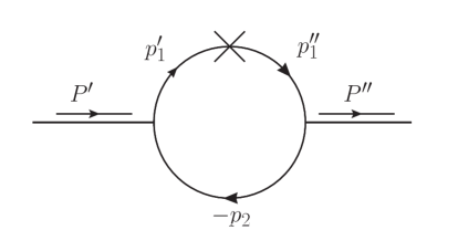
Figure 3: The one-loop Feynman diagram for meson weak transition amplitude, where $P^{\prime}(P^{\prime\prime})$ is the momentum of the incoming (outgoing) meson, $p_{1}^{\prime(\prime\prime)}$ and $p_{2}$ are the momenta of the quark and antiquark, respectively. The symbol “cross” denotes the weak interaction vertex.

According to Refs. Cheng:2003sm ; Zhang:2023ypl , the corresponding weak transition matrix element at the one-loop level can be calculated in terms of the Feynman loop integral, as shown in Fig. 3. Then the form factors can be extracted from the corresponding matrix element. To write down the transition amplitude, we need the meson-quark antiquark vertices for the initial meson as $i\Gamma^{\prime}=H_{P}^{\prime}\gamma_{5}$, and that of the outgoing meson as $i(\gamma_{0}\Gamma^{\prime\prime\dagger}\gamma_{0})$ with $\Gamma^{\prime\prime}=H_{V}^{\prime\prime}\big{[}\gamma_{\mu}-(p_{1}^{\prime\prime}-p_{2})_{\mu}/W_{V}^{\prime\prime}\big{]}$ Cheng:2003sm ; Zhang:2023ypl , where the subscripts $P$ and $V$ denote the pseudoscalar and vector meson, respectively.

For Fig. 3, the concrete expression of the transition amplitude for $P\to V$ can be expressed as

$$\begin{split}\mathcal{B}_{\mu}^{V(A,T,T\text{5})}=-i^{3}\frac{N_{c}}{(2\pi)^{4}}\int d^{4}p_{1}^{\prime}\frac{iH_{P}^{\prime}H_{V}^{\prime\prime}}{N_{1}^{\prime}N_{1}^{\prime\prime}N_{2}}S_{\mu\nu}^{V(A,T,T\text{5})}\epsilon_{V}^{*\nu},\end{split}$$ (3.6)

where $N_{1}^{\prime(\prime\prime)}=p_{1}^{\prime(\prime\prime)2}-m_{1}^{\prime(\prime\prime)2}$ and $N_{2}=p_{2}^{2}-m_{2}^{2}$ come from the propagators of the quarks. The superscripts $V$, $A$, $T$, and $T\text{5}$ represent the vector, axial-vector, tensor, and pseudotensor currents, respectively. The traces $S_{\mu\nu}^{V}$ are written as

$$\begin{split}S_{\mu\nu}^{V}{\!}=&\text{Tr}\Big{[}\Big{(}\gamma_{\nu}{\!}-{\!}\frac{(p_{1}^{\prime\prime}{\!}-{\!}p_{2})_{\nu}}{W_{V}^{\prime\prime}}\Big{)}(\not{p}_{1}^{\prime\prime}+m_{1}^{\prime\prime})\gamma_{\mu}(\not{p}_{1}^{\prime}+m_{1}^{\prime})\gamma_{5}(-\not{p}_{2}+m_{2})\Big{]}\\ =&-2i\epsilon_{\mu\nu\alpha\beta}\bigg{[}p_{1}^{\prime\alpha}P^{\beta}(m_{1}^{\prime\prime}-m_{1}^{\prime})+p_{1}^{\prime\alpha}q^{\beta}(m_{1}^{\prime\prime}+m_{1}^{\prime}-2m_{2})\\ &+q^{\alpha}P^{\beta}m_{1}^{\prime}\bigg{]}+\frac{1}{W_{V}^{\prime\prime}}(4p_{1\nu}^{\prime}-3q_{\nu}-P_{\nu})i\epsilon_{\mu\alpha\beta\rho}p_{1}^{\prime\alpha}q^{\beta}P^{\rho}.\end{split}$$ (3.7)

To make reading easier, the relevant expressions of the traces $S_{\mu\nu}^{A,T,T5}$ are collected in Appendix A.

Following Refs. Cheng:2003sm ; Cheng:2004yj ; Cheng:2009ms , the execution of the $p_{1}^{\prime-}$ integration went to the replacement:

$$\begin{split}N_{1}^{\prime(\prime\prime)}&\to\hat{N}_{1}^{\prime(\prime\prime)}=x_{1}\big{(}M^{\prime(\prime\prime)2}-M_{0}^{\prime(\prime\prime)2}\big{)},\\ H_{P(V)}^{\prime(\prime\prime)}&\to h_{P(V)}^{\prime(\prime\prime)},\\ W_{V}^{\prime\prime}&\to\omega_{V}^{\prime\prime},\\ \int\frac{d^{4}p_{1}^{\prime}}{(2\pi)^{4}}H_{P}^{\prime}H_{V}^{\prime\prime}S_{\mu\nu}\epsilon^{*\nu}&\to-i\pi\int\frac{dx_{2}d^{2}\vec{k}_{\bot}^{\prime}}{x_{2}\hat{N}_{1}^{\prime}\hat{N}_{1}^{\prime\prime}}h_{P}^{\prime}h_{V}^{\prime\prime}\hat{S}_{\mu\nu}\epsilon^{*\nu},\end{split}$$ (3.8)

where we define

$$M_{0}^{\prime(\prime\prime)2}=\frac{\vec{k}_{\bot}^{\prime(\prime\prime)2}+m_{1}^{\prime(\prime\prime)2}}{x_{1}}+\frac{\vec{k}_{\bot}^{\prime(\prime\prime)2}+m_{2}^{\prime(\prime\prime)2}}{x_{2}},$$ (3.9)

with $\vec{k}_{\bot}^{\prime\prime}=\vec{k}_{\bot}^{\prime}-x_{2}\vec{q}_{\bot}$ and $\omega_{V}^{\prime\prime}=M_{0}^{\prime\prime}+m_{1}^{\prime\prime}+m_{2}$.

To write down the concrete expression of $\hat{S}_{\mu\nu}$, we should take into account the so-called zero-mode contribution. As shown in Refs. Cheng:2003sm ; Chen:2017vgi , after doing the integration in Eq. (3.8) we have $p_{2}=\hat{p}_{2}$, and

$$\begin{split}\hat{p}_{1}^{\prime\mu}&=(P^{\prime}-\hat{p}_{2})^{\mu}\\ &=x_{1}P^{\prime\mu}+(0,0,\vec{k}_{\bot}^{\prime})^{\mu}+\frac{1}{2}\Big{(}x_{2}P^{\prime-}-\frac{\vec{p}_{2\bot}^{2}+m_{2}^{2}}{x_{2}P^{\prime+}}\Big{)}\tilde{\omega}^{\mu},\end{split}$$ (3.10)

where $\tilde{\omega}=(2,0,\vec{0}_{\bot})$ is a lightlike four vector in the light-front coordinate. Following the discussions in a series of papers Cheng:2003sm ; Cheng:2004yj ; Cheng:2009ms ; Chen:2017vgi , for avoiding the $\tilde{\omega}$ dependence, we need to do the following replacements Cheng:2003sm ; Cheng:2004yj ; Cheng:2009ms :

$$\begin{split}\hat{p}_{1\mu}^{\prime}{\!}\doteq&P_{\mu}A_{1}^{(1)}+q_{\mu}A_{2}^{(1)},\\ \hat{p}_{1\mu}^{\prime}\hat{p}_{1\nu}^{\prime}{\!}\doteq&g_{\mu\nu}A_{1}^{(2)}{\!}+{\!}P_{\mu}P_{\nu}A_{2}^{(2)}{\!}+{\!}(P_{\mu}q_{\nu}{\!}+{\!}P_{\nu}q_{\mu})A_{3}^{(2)}{\!}+{\!}q_{\mu}q_{\nu}A_{4}^{(2)},\\ N_{2}\doteq&Z_{2},\\ \hat{p}_{1\mu}^{\prime}\hat{N}_{2}{\!}\doteq&q_{\mu}\Big{(}A_{2}^{(1)}Z_{2}+\frac{P\cdot q}{q^{2}}A_{1}^{(2)}\Big{)},\\ \hat{p}_{1\mu}^{\prime}\hat{p}_{1\nu}^{\prime}\hat{N}_{2}{\!}\doteq&g_{\mu\nu}A_{1}^{(2)}Z_{2}+q_{\mu}q_{\nu}\Big{[}A_{4}^{(2)}Z_{2}+2\frac{P\cdot q}{q^{2}}A_{2}^{(1)}A_{1}^{(2)}\Big{]},\end{split}$$ (3.11)

in Eqs. (3.7),  (A.1),  (A.4), and  (A.5). Here, $Z_{2}=\hat{N}_{1}^{\prime}+m_{1}^{\prime 2}-m_{2}^{2}+(1-2x_{1})M^{\prime 2}+(q^{2}+P\cdot q)\frac{\vec{k}_{\bot}^{\prime}\cdot\vec{q}_{\bot}}{q^{2}}$, $P\cdot q=M^{\prime 2}-M^{\prime\prime 2}$, and

$$\begin{split}A_{1}^{(1)}&=\frac{x_{1}}{2},~{}~{}~{}A_{2}^{(1)}=A_{1}^{(1)}-\frac{\vec{k}_{\bot}^{\prime}\cdot\vec{q}_{\bot}}{q^{2}},\\ A_{1}^{(2)}&=-\vec{k}_{\bot}^{\prime 2}-\frac{(\vec{k}_{\bot}^{\prime}\cdot\vec{q}_{\bot})^{2}}{q^{2}},~{}~{}~{}A_{2}^{(2)}=(A_{1}^{(1)})^{2},\\ A_{3}^{(2)}&=A_{1}^{(1)}A_{2}^{(1)},~{}~{}~{}A_{4}^{(2)}=(A_{2}^{(1)})^{2}-\frac{1}{q^{2}}A_{1}^{(2)}.\end{split}$$ (3.12)

After performing the replacements (3.11) in the decay amplitudes (3.7) and (A.1), the form factors $g$, $f$, $a_{+}$, and $a_{-}$ can be obtained from the terms proportional to the $\epsilon_{\mu\nu\alpha\beta}P^{\alpha}q^{\beta}$, $g_{\mu\nu}$, $P_{\mu}P_{\nu}$ and $P_{\mu}q_{\nu}$, and $q_{\mu}P_{\nu}$ and $q_{\mu}q_{\nu}$, respectively. The $\epsilon_{V}^{*\mu}P^{\prime\prime}_{\mu}=0$ is used here. Finally, the expressions of these form factors in covariant LFQMs can be written as Jaus:1999zv ; Cheng:2003sm ; Zhang:2023ypl

$$\begin{split}g(q^{2})=&-\frac{N_{c}}{16\pi^{3}}\int dx_{2}d^{2}\vec{k}_{2\bot}\frac{2h_{P}^{\prime}h_{V}^{\prime\prime}}{x_{2}\hat{N}_{1}^{\prime}\hat{N}_{1}^{\prime\prime}}\Bigg{\{}x_{2}m_{1}^{\prime}+x_{1}m_{2}+(m_{1}^{\prime}-m_{1}^{\prime\prime})\frac{k_{\bot}^{\prime}\cdot q_{\bot}}{q^{2}}+\frac{2}{\omega_{V}^{\prime\prime}}\Big{[}k_{\bot}^{\prime 2}+\frac{(k_{\bot}^{\prime}\cdot q_{\bot})^{2}}{q^{2}}\Big{]}\Bigg{\}},\end{split}$$ (3.13)

$$\begin{split}f(q^{2})=&\frac{N_{c}}{16\pi^{3}}\int dx_{2}d^{2}\vec{k}_{\bot}^{\prime}\frac{h_{P}^{\prime}h_{V}^{\prime\prime}}{x_{2}\hat{N}_{1}^{\prime}\hat{N}_{1}^{\prime\prime}}\Bigg{\{}2x_{1}(m_{2}-m_{1}^{\prime})(M_{0}^{\prime 2}+M_{0}^{\prime\prime 2})-4x_{1}m_{1}^{\prime\prime}M_{0}^{\prime 2}+2x_{2}m_{1}^{\prime}P\cdot q+2m_{2}q^{2}\\ &-2x_{1}m_{2}(M^{\prime 2}+M^{\prime\prime 2})+2(m_{1}^{\prime}-m_{2})(m_{1}^{\prime}+m_{1}^{\prime\prime})^{2}+8(m_{1}^{\prime}-m_{2})\Big{[}k_{\bot}^{\prime 2}+\frac{(k_{\bot}^{\prime}\cdot q_{\bot})^{2}}{q^{2}}\Big{]}\\ &+2(m_{1}^{\prime}+m_{1}^{\prime\prime})(q^{2}+P\cdot q)\frac{k_{\bot}^{\prime}\cdot q_{\bot}}{q^{2}}-4\frac{q^{2}k_{\bot}^{\prime 2}+(k_{\bot}^{\prime}\cdot q_{\bot})^{2}}{q^{2}\omega_{V}^{\prime\prime}}\Big{[}2x_{1}(M^{\prime 2}+M_{0}^{\prime 2})-q^{2}-P\cdot q\\ &-2(q^{2}+P\cdot q)\frac{k_{\bot}^{\prime}\cdot q_{\bot}}{q^{2}}-2(m_{1}^{\prime}-m_{1}^{\prime\prime})(m_{1}^{\prime}-m_{2})\Big{]}\Bigg{\}},\end{split}$$ (3.14)

$$\begin{split}a_{+}(q^{2})=&\frac{N_{c}}{16\pi^{3}}\int dx_{2}d^{2}\vec{k}_{\bot}^{\prime}\frac{2h_{P}^{\prime}h_{V}^{\prime\prime}}{x_{2}\hat{N}_{1}^{\prime}\hat{N}_{1}^{\prime\prime}}\Bigg{\{}(x_{1}-x_{2})(x_{2}m_{1}^{\prime}+x_{1}m_{2})-\big{[}2x_{1}m_{2}+m_{1}^{\prime\prime}+(x_{2}-x_{1})m_{1}^{\prime}\big{]}\frac{k_{\bot}^{\prime}\cdot q_{\bot}}{q^{2}}\\ &-2\frac{x_{2}q^{2}+k_{\bot}^{\prime}\cdot q_{\bot}}{x_{2}q^{2}\omega_{V}^{\prime\prime}}\big{[}k_{\bot}^{\prime}\cdot k_{\bot}^{\prime\prime}+(x_{1}m_{2}+x_{2}m_{1}^{\prime})(x_{1}m_{2}-x_{2}m_{1}^{\prime\prime})\big{]}\Bigg{\}},\end{split}$$ (3.15)

$$\begin{split}a_{-}(q^{2})=&\frac{N_{c}}{16\pi^{3}}\int dx_{2}d^{2}\vec{k}_{\bot}^{\prime}\frac{h_{P}^{\prime}h_{V}^{\prime\prime}}{x_{2}\hat{N}_{1}^{\prime}\hat{N}_{1}^{\prime\prime}}\Bigg{\{}2(2x_{1}-3)(x_{2}m_{1}^{\prime}+x_{1}m_{2})-8(m_{1}^{\prime}-m_{2})\Big{[}\frac{k_{\bot}^{\prime 2}}{q^{2}}+2\frac{(k_{\bot}^{\prime}\cdot q_{\bot})^{2}}{q^{4}}\Big{]}\\ &-\big{[}(14-12x_{1})m_{1}^{\prime}-2m_{1}^{\prime\prime}-(8-12x_{1})m_{2}\big{]}\frac{k_{\bot}^{\prime}\cdot q_{\bot}}{q^{2}}+\frac{4}{\omega_{V}^{\prime\prime}}\Big{(}\big{[}M^{\prime 2}+M^{\prime\prime 2}-q^{2}+2(m_{1}^{\prime}-m_{2})(m_{1}^{\prime\prime}+m_{2})\big{]}\\ &\times(A_{3}^{2}+A_{4}^{(2)}-A_{2}^{1})+Z_{2}(3A_{2}^{(1)}-2A_{4}^{(2)}-1)+\frac{1}{2}P\cdot q(A_{1}^{(1)}+A_{2}^{(1)}-1)\big{[}x_{1}(q^{2}+P\cdot q)-2M^{\prime 2}-2k_{\bot}^{\prime}\cdot q_{\bot}\\ &-2m_{1}^{\prime}(m_{1}^{\prime\prime}+m_{2}-2m_{2}(m_{1}^{\prime}-m_{2}))\big{]}\Big{[}\frac{k_{\bot}^{\prime 2}}{q^{2}}+\frac{(k_{\bot}^{\prime}\cdot q_{\bot})^{2}}{q^{4}}\Big{]}(4A_{2}^{(1)}-3)\Big{)}\Bigg{\}},\end{split}$$ (3.16)

The form factors deduced by (axial)vector currents defined in Eq. (3.2) can thus be evaluated by

$$\begin{split}V(q^{2})=&-(M^{\prime}+M^{\prime\prime})g(q^{2}),\\ A_{0}(q^{2})=&-\frac{1}{2M^{\prime\prime}}f(q^{2})-\frac{M^{\prime 2}-M^{\prime\prime 2}}{2M^{\prime\prime}}a_{+}(q^{2})-\frac{q^{2}}{2M^{\prime\prime}}a_{-}(q^{2}),\\ A_{1}(q^{2})=&-f(q^{2})/(M^{\prime}+M^{\prime\prime}),~{}~{}~{}A_{2}(q^{2})=(M^{\prime}+M^{\prime\prime})a_{+}(q^{2}).\end{split}$$ (3.17)

Analogously, we can obtain the concrete expressions of the (pseudo)tensor form factors defined in Eq. (3.4) as Cheng:2009ms

$$\begin{split}T_{1}(q^{2})=&\frac{N_{c}}{16\pi^{3}}\int dx_{2}d^{2}\vec{k}_{\bot}^{\prime}\frac{h_{P}^{\prime}h_{V}^{\prime\prime}}{x_{2}\hat{N}_{1}^{\prime}\hat{N}_{1}^{\prime\prime}}\Bigg{\{}2A_{1}^{(1)}[M^{\prime 2}-M^{\prime\prime 2}-2m_{1}^{\prime 2}-2\hat{N}_{1}^{\prime}+q^{2}+2(m_{1}^{\prime}m_{2}+m_{1}^{\prime\prime}m_{2}-m_{1}^{\prime}m_{1}^{\prime\prime})]\\ &-8A_{1}^{(2)}+(m_{1}^{\prime}+m_{1}^{\prime\prime})^{2}+\hat{N}_{1}^{\prime}+\hat{N}_{1}^{\prime\prime}-q^{2}+4(M^{\prime 2}-M^{\prime\prime 2})(A_{2}^{(2)}-A_{3}^{(2)})+4q^{2}(-A_{1}^{(1)}+A_{2}^{(1)}+A_{3}^{(2)}-A_{4}^{(2)})\\ &-\frac{4}{\omega_{V}^{\prime\prime}}(m_{1}^{\prime}+m_{1}^{\prime\prime})A_{1}^{(2)}\Bigg{\}},\end{split}$$ (3.18)

$$\begin{split}T_{2}(q^{2})=&T_{1}(q^{2})+\frac{q^{2}}{M^{\prime 2}-M^{\prime\prime 2}}\frac{N_{c}}{16\pi^{3}}\int dx_{2}d^{2}\vec{k}_{\bot}^{\prime}\frac{h_{P}^{\prime}h_{V}^{\prime\prime}}{x_{2}\hat{N}_{1}^{\prime}\hat{N}_{1}^{\prime\prime}}\Bigg{\{}2A_{2}^{(1)}[M^{\prime 2}-M^{\prime\prime 2}-2m_{1}^{\prime 2}-2\hat{N}_{1}^{\prime}+q^{2}\\ &+2(m_{1}^{\prime}m_{2}+m_{1}^{\prime\prime}m_{2}-m_{1}^{\prime}m_{1}^{\prime\prime})]-8A_{1}^{(2)}-2M^{\prime 2}+2m_{1}^{\prime 2}+(m_{1}^{\prime}+m_{1}^{\prime\prime})^{2}+2(m_{2}-2m_{1}^{\prime})m_{2}+3\hat{N}_{1}^{\prime}+\hat{N}_{1}^{\prime\prime}\\ &-q^{2}+2Z_{2}+4(q^{2}-2M^{\prime 2}-2M^{\prime\prime 2})(A_{2}^{(2)}-A_{3}^{(2)})-4(M^{\prime 2}-M^{\prime\prime 2})(-A_{1}^{(1)}+A_{2}^{(1)}+A_{3}^{(2)}-A_{4}^{(2)})\\ &-\frac{4}{\omega_{V}^{\prime\prime}}(m_{1}^{\prime\prime}-m_{1}^{\prime}+2m_{2})A_{1}^{(2)}\Bigg{\}},\end{split}$$ (3.19)

$$\begin{split}T_{3}(q^{2})=&\frac{N_{c}}{16\pi^{3}}\int dx_{2}d^{2}\vec{k}_{\bot}^{\prime}\frac{h_{P}^{\prime}h_{V}^{\prime\prime}}{x_{2}\hat{N}_{1}^{\prime}\hat{N}_{1}^{\prime\prime}}\Bigg{\{}-2A_{2}^{(1)}[M^{\prime 2}-M^{\prime\prime 2}-2m_{1}^{\prime 2}-2\hat{N}_{1}^{\prime}+q^{2}+2(m_{1}^{\prime}m_{2}+m_{1}^{\prime\prime}m_{2}-m_{1}^{\prime}m_{1}^{\prime\prime})]\\ &+8A_{1}^{(2)}+2M^{\prime 2}-2m_{1}^{\prime 2}-(m_{1}^{\prime}+m_{1}^{\prime\prime})^{2}-2(m_{2}-2m_{1}^{\prime})m_{2}-3\hat{N}_{1}^{\prime}-\hat{N}_{1}^{\prime\prime}+q^{2}-2Z_{2}-4(q^{2}-M^{\prime 2}-3M^{\prime\prime 2})\\ &\times(A_{2}^{(2)}-A_{3}^{(2)})+\frac{4}{\omega_{V}^{\prime\prime}}\Big{(}(m_{1}^{\prime\prime}-m_{1}^{\prime}+2m_{2})[A_{1}^{(2)}+(M^{\prime 2}-M^{\prime\prime 2})(A_{2}^{(2)}+A_{3}^{(2)}-A_{1}^{(1)})]\\ &+(m_{1}^{\prime}+m_{1}^{\prime\prime})(M^{\prime 2}-M^{\prime\prime 2})(A_{2}^{(1)}-A_{3}^{(2)}-A_{4}^{(2)})+m_{1}^{\prime}(M^{\prime 2}-M^{\prime\prime 2})(A_{1}^{(1)}+A_{2}^{(1)}-1)\Big{)}\Bigg{\}}.\end{split}$$ (3.20)

Following the treatment in Ref. Cheng:2003sm , $h_{M}$ is taken as

$$\begin{split}h_{P}^{\prime}=&(M^{\prime 2}-M_{0}^{\prime 2})\sqrt{\frac{x_{1}x_{2}}{N_{c}}}\frac{1}{\sqrt{2}\tilde{M}_{0}^{\prime}}\phi_{s}(x_{2},\vec{k}_{\bot}^{\prime}),\\ h_{V}^{\prime\prime}=&(M^{\prime\prime 2}-M_{0}^{\prime\prime 2})\sqrt{\frac{x_{1}x_{2}}{N_{c}}}\frac{1}{\sqrt{2}\tilde{M}_{0}^{\prime\prime}}\phi_{s}(x_{2},\vec{k}_{\bot}^{\prime\prime}),\end{split}$$ (3.21)

where $\tilde{M}_{0}^{\prime(\prime\prime)}=\sqrt{M_{0}^{\prime(\prime\prime)2}-(m_{1}^{\prime(\prime\prime)}-m_{2})^{2}}$, and $\phi_{s}$ is the space wave function of the pseudoscalar or vector meson.

In the previous theoretical work Cheng:2003sm ; Zhang:2023ypl , the phenomenological Gaussian-type wave functions

$$\phi_{s}(x_{2},\vec{k}_{\bot}^{\prime(\prime\prime)})=4\Big{(}\frac{\pi}{\beta^{\prime(\prime\prime)2}}\Big{)}^{3/4}{\!}\sqrt{\frac{e_{1}^{\prime(\prime\prime)}e_{2}}{x_{1}x_{2}M_{0}^{\prime(\prime\prime)}}}\exp\Big{(}{\!}-{\!}\frac{\vec{k}_{\bot}^{\prime(\prime\prime)2}+k_{z}^{\prime(\prime\prime)2}}{2\beta^{\prime(\prime\prime)2}}\Big{)},$$ (3.22)

with

$$\begin{split}k_{z}^{\prime(\prime\prime)}&=\frac{x_{2}M_{0}^{\prime(\prime\prime)}}{2}-\frac{m_{2}^{2}+\vec{k}_{\bot}^{\prime(\prime\prime)2}}{2x_{2}M_{0}^{\prime(\prime\prime)}},\\ e_{1}^{\prime(\prime\prime)}&=\sqrt{m_{1}^{\prime(\prime\prime)2}+\vec{k}_{\bot}^{\prime(\prime\prime)2}+k_{z}^{\prime(\prime\prime)2}},\\ e_{2}&=\sqrt{m_{2}^{2}+\vec{k}_{\bot}^{\prime 2}+k_{z}^{\prime 2}},\end{split}$$ (3.23)

are widely used. It inevitably introduces the dependence of the parameter $\beta$. The phenomenological parameter $\beta$ can be fixed by the decay constant Cheng:2003sm ; Cheng:2004yj ; Cheng:2009ms . However, as we all know, the decay constant is only associated with the meson wave function at the end point $q^{2}=0$. This indicates that the simple wave function Eq. (3.22) deviating from the $q^{2}=0$ region may be unreliable.

Taking advantage of the modified GI model Li:2023wgq , we can obtain the numerical spatial wave functions of the mesons concerned. By replacing the form in Eq. (3.22) with

$$\begin{split}\phi_{l}(x_{2},\vec{k}_{\bot}^{\prime(\prime\prime)})&=\sqrt{4}\pi\sum_{n=1}^{N_{\text{max}}}c_{n}\sqrt{\frac{e_{1}^{\prime(\prime\prime)}e_{2}}{x_{1}x_{2}M_{0}^{\prime(\prime\prime)}}}R_{nl}\Big{(}\sqrt{\vec{k}_{\bot}^{\prime(\prime\prime)2}+k_{z}^{\prime(\prime\prime)2}}\Big{)},\\ \phi_{s}(x_{2},\vec{k}_{\bot}^{\prime(\prime\prime)})&\equiv\phi_{l=0}(x_{2},\vec{k}_{\bot}^{\prime(\prime\prime)}),\end{split}$$ (3.24)

where $c_{n}$ are the expansion coefficients of the corresponding eigenvectors and $l$ is the orbital angular momentum of the meson, we can avoid the corresponding uncertainty. In Table 3, we collect the expansion coefficients $c_{n}$ of the meson wave functions involved. In addition, the factor $\sqrt{4}\pi$ is needed to satisfy the normalization:

$$\int\frac{dx_{2}d\vec{k}_{\bot}}{2(2\pi)^{3}}\phi_{l}^{*}(x_{2},\vec{k}_{\bot})\phi_{l}(x_{2},\vec{k}_{\bot})=1.$$ (3.25)

Besides, the $R_{nl}$ is the simple harmonic oscillator wave function as

$$R_{nl}(|p|){\!}={\!}\frac{(-1)^{n-1}}{\beta^{3/2}}{\!}\sqrt{\frac{2(n-1)!}{\Gamma(n{\!}+{\!}l{\!}+{\!}1/2)}}\Bigg{(}\frac{p}{\beta}\Bigg{)}^{l}\exp\Bigg{(}{\!}-{\!}\frac{p^{2}}{2\beta^{2}}\Bigg{)}L_{n{\!}-{\!}1}^{l}\Bigg{(}\frac{p^{2}}{\beta^{2}}\Bigg{)}.$$ (3.26)

The parameter $\beta=0.5\ \text{GeV}$ in the above equation is consistent with Ref. Li:2023wgq .

Table 3: The calculated masses and the expansion coefficients $c_{n}$ of the wave function of the mesons involved Li:2023wgq . The masses are given in units of MeV.

States	Masses Li:2023wgq	Experiments ParticleDataGroup:2022pth	Eigenvector coefficients $c_{n}$ Li:2023wgq
$B_{c}$	$6271$	$6274.47\pm 0.32$	$\Big{\{}0.7877,0.4410,0.2857,0.1991,0.1470,0.1132,0.0900,0.0734,0.0611,0.0517,$
			$0.0444,0.0385,0.0338,0.0299,0.0266,0.0238,0.0215,0.0195,0.0177,0.0162,$
			$0.0148,0.0136,0.0125,0.0116,0.0107,0.0099,0.0092,0.0084,0.0081,0.0066,0.0081\Big{\}}$
$D_{s}^{*}$	$2112$	$2112.2\pm 0.4$	$\Big{\{}0.9708,0.16203,0.1515,0.0605,0.0518,0.0286,0.0240,0.0156,0.0130,0.0093,$
			$0.0078,0.0059,0.0050,0.0039,0.0033,0.0027,0.0023,0.0019,0.0016,0.0013$
			$0.0012,0.0010,0.0008,0.0007,0.0006,0.0005,0.0005,0.0004,0.0003,0.0003,0.0003\Big{\}}$

IV Numerical results and discussions

IV.1 The form factors

With the input of the numerical wave functions, and the concrete expressions of the seven form factors in Eqs. (3.13)-(3.20), we present in this subsection the numerical results of $B_{c}\to D_{s}^{*}$ form factors.

Following the approach described in Refs. Jaus:1999zv ; Cheng:2003sm , we assume the condition $q^{+}=0$. This implies that our form factor calculations are performed in the spacelike region ($q^{2}<0$), and therefore we need to extrapolate them to the timelike region ($q^{2}>0$). To perform the analytical continuation, we utilize the $z$-series parametrization Chen:2017vgi

$$\begin{split}\mathcal{F}(q^{2}){\!}=&{\!}\frac{\mathcal{F}(0)}{1{\!}-{\!}q^{2}/m_{\text{pole}}^{2}}\Bigg{\{}1{\!}+{\!}a_{1}\Big{(}z(q^{2}){\!}-{\!}z(0){\!}-{\!}\frac{1}{3}\big{[}z(q^{2})^{2}{\!}-{\!}z(0)^{2}\big{]}\Big{)}\\ &+a_{2}\Big{(}z(q^{2}){\!}-{\!}z(0){\!}+{\!}\frac{2}{3}\big{[}z(q^{2})^{2}{\!}-{\!}z(0)^{2}\big{]}\Big{)}\Bigg{\}},\end{split}$$ (4.1)

where $a_{i}$ ($i$ = 1, 2) are free parameters needed to fit in the $q^{2}<0$ region, and the $z(q^{2})$ is taken as

$$z(q^{2})=\frac{\sqrt{t_{+}-q^{2}}-\sqrt{t_{+}-t_{0}}}{\sqrt{t_{+}-q^{2}}+\sqrt{t_{+}-t_{0}}}$$ (4.2)

with $t_{\pm}=(M^{\prime}\pm M^{\prime\prime})^{2}$ and $t_{0}=t_{+}\Big{(}1-\sqrt{1-t_{-}/t_{+}}\Big{)}$.

To determine the values of the free parameters $a_{i}$, as given in Eq. (4.1), we perform numerical calculations at 200 equally spaced points for each form factor, ranging from $-20$ to $-0.1\ \text{GeV}^{2}$, using Eqs. (3.13)-(3.20). The calculated points are then fitted using Eq. (4.1). The fitted values of the free parameters, as well as $\mathcal{F}(0)$, $\mathcal{F}(q_{\text{max}}^{2})$, and the pole masses, are listed in Table 4. Additionally, the $q^{2}$ dependence of the transition form factors $B_{c}\to D_{s}^{*}$ is shown in Fig. 4.

Table 4: Our results of the weak transition form factors of $B_{c}\to D_{s}^{*}$ by using the covariant LFQM.

	$\mathcal{F}(0)$	$\mathcal{F}(q_{\text{max}}^{2})$	$m_{\text{pole}}$ (GeV)	$a_{1}$	$a_{2}$
$V^{B_{c}\to B_{s}^{*}}$	$0.434$	$1.652$	$5.415$	$-7.909$	$15.667$
$A_{0}^{B_{c}\to B_{s}^{*}}$	$0.387$	$1.436$	$5.367$	$-6.790$	$9.427$
$A_{1}^{B_{c}\to B_{s}^{*}}$	$0.274$	$0.588$	$5.829$	$-0.721$	$-4.299$
$A_{2}^{B_{c}\to B_{s}^{*}}$	$0.159$	$0.438$	$5.829$	$-4.942$	$5.168$
$T_{1}^{B_{c}\to B_{s}^{*}}$	$0.265$	$1.050$	$5.415$	$-8.821$	$19.272$
$T_{2}^{B_{c}\to B_{s}^{*}}$	$0.265$	$0.424$	$5.829$	$3.067$	$-9.950$
$T_{3}^{B_{c}\to B_{s}^{*}}$	$0.231$	$0.637$	$5.829$	$-4.985$	$4.566$

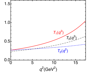
Figure 4: The $q^{2}$ dependence of the $B_{c}\to{D}_{s}^{*}$ weak transition form factors. Here, the four dependent form factors deduced by (axial)vector are presented in the left panel, while the three dependent ones deduced by (pseudo)tensor are shown in the right panel.

In Table 5, we compare our results for the $B_{c}\to{D}_{s}^{*}$ weak transition form factors at the end point $q^{2}=0$ with other approaches, in which Refs. Kiselev:2002vz ; Azizi:2008vv calculated the concerned form factors with the QCD sum rule, Refs. Geng:2001vy ; Wang:2008xt ; Zhang:2023ypl used the covariant LFQM, and Ref. Dhir:2008hh used the Bauer-Stech-Wirbel model and considered the effects of flavor dependence on the form factors caused by possible variation of the average transverse quark momentum ($\omega$) inside the meson. In addition, Ref. Geng:2001vy also used the CQM, and Ref. Wang:2014yia used the pQCD approach. References Geng:2001vy ; Wang:2014yia ; Azizi:2008vv contain the results of (pseudo)tensor form factors. Obviously, our results of the (pseudo)tensor form factors, i.e., $T_{1,2,3}$, at the end point $q^{2}=0$ are consistent with the predictions of pQCD Wang:2014yia and the LFQM Geng:2001vy . We expect further theoretical work, especially LQCD, which is useful to constrain the behavior of the form factors in the low-recoiling region, to test our results.

Table 5: Theoretical predictions of the $B_{c}\to{D}_{s}^{*}$ transition form factors at the end point $q^{2}=0$ using different approaches.

	$V^{B_{c}\to{D}_{s}^{*}}(0)$	$A_{0}^{B_{c}\to{D}_{s}^{*}}(0)$	$A_{1}^{B_{c}\to{D}_{s}^{*}}(0)$	$A_{2}^{B_{c}\to{D}_{s}^{*}}(0)$	$T_{1}^{B_{c}\to{D}_{s}^{*}}(0)$	$T_{2}^{B_{c}\to{D}_{s}^{*}}(0)$	$T_{3}^{B_{c}\to{D}_{s}^{*}}(0)$
This work	$0.434$	$0.387$	$0.274$	$0.159$	$0.265$	$0.265$	$0.231$
Ref. Kiselev:2002vz	$2.02$	$0.47$	$0.56$	$0.65$	$\cdots$	$\cdots$	$\cdots$
Ref. Dhir:2008hh [1]	$0.032$	$0.016$	$0.015$	$0.013$	$\cdots$	$\cdots$	$\cdots$
Ref. Dhir:2008hh [2]	$0.29^{+0.02}_{-0.03}$	$0.16^{+0.01}_{-0.01}$	$0.18^{+0.01}_{-0.02}$	$0.20^{+0.02}_{-0.03}$	$\cdots$	$\cdots$	$\cdots$
Ref. Wang:2008xt	$0.23^{+0.04}_{-0.03}$	$0.17^{+0.01}_{-0.01}$	$0.14^{+0.02}_{-0.01}$	$0.12^{+0.02}_{-0.02}$	$\cdots$	$\cdots$	$\cdots$
Ref. Zhang:2023ypl	$0.25^{+0.00}_{-0.00}$	$0.18^{+0.02}_{-0.03}$	$0.16^{+0.01}_{-0.02}$	$0.15^{+0.01}_{-0.01}$	$\cdots$	$\cdots$	$\cdots$
Ref. Geng:2001vy	$0.336$	$0.164$	$0.118$	$\cdots$	$0.214$	$0.214$	$\cdots$
Ref. Geng:2001vy	$0.262$	$0.139$	$0.144$	$\cdots$	$0.167$	$0.167$	$\cdots$
Ref. Azizi:2008vv	$0.54\pm 0.018$	$0.30\pm 0.017$	$0.36\pm 0.013$	$\cdots$	$0.31\pm 0.017$	$0.33\pm 0.016$	$0.29\pm 0.034$
Ref. Wang:2014yia	$0.33\pm 0.06$	$0.21\pm 0.04$	$0.23\pm 0.04$	$0.25\pm 0.05$	$0.28\pm 0.06$	$0.28\pm 0.06$	$0.27\pm 0.06$

• These results, listed in the fourth row, are obtained by using the universe parameter $\omega=0.40$ GeV.

• These results, listed in the fifth row, are obtained by using different parameters, i.e., $\omega=0.96^{+0.08}_{-0.07}$ GeV for the $B_{c}$ meson and $\omega=0.51$ GeV for the $D_{s}^{*}$ meson.

IV.2 The angular distributions and physical observables

With the above preparations, in this subsection we present our numerical results of the branching fractions and some angular observables, i.e., the $CP$-averaged normalized angular coefficients $S_{i}$, the lepton’s forward-backward asymmetry parameter $A_{FB}$, and the longitudinal (transverse) polarization fractions of the $D_{s}^{*}$ meson $F_{L(T)}$. In addition, we also investigate the clean angular observables $P_{1,2,3}$ and $P^{\prime}_{4,5,6,8}$. The hadron and lepton masses are quoted from the PDG ParticleDataGroup:2022pth , as well as the lifetime $\tau_{B_{c}}=0.510$ps and the branching fraction $\mathcal{B}(D_{s}^{*}\to{D}_{s}\pi)=5\%$.

First, we focus on the angular coefficients $S_{i}$ and $A_{i}$ defined in Eq. (LABEL:eq:SiAi). The $q^{2}$ dependence of the normalized $CP$-averaged angular coefficients $S_{i}$ are presented in Fig. 5, while the $CP$ asymmetry angular coefficients $A_{i}$ are shown in Fig. 6. The blue dashed lines and the magenta solid lines represent the muon and the tau channels, respectively. Since the electron channel shows similar behavior to the muon channel, we will only present our results for the muon and the tau channels here. In the energy regions of $8.0<q^{2}<11.0$ and $12.5<q^{2}<15.0~{}\text{GeV}^{2}$, we use the gray areas to mark the contributions from the charmonium states $J/\psi$ and $\psi(2S)$. In our calculation, we adopted phenomenological and model-dependent treatment, i.e., the Breit-Wigner ansatz to model the corresponding contribution. In the experiment, these two regions are generally truncated. The $CP$ asymmetry angular coefficients, $A_{i}$, are shown to be very small in the SM, due to the direct $CP$ violation being proportional to the $\text{Im}[V_{ub}V_{us}^{*}/V_{tb}V_{ts}^{*}]$, which is around $10^{-2}$. This character is very clear in Fig. 6. Also, the $S_{7,8,9}$ are also very small compared to the other angular coefficients $S_{i}$. These angular coefficients are important physical observables to reveal the underlying decay mechanism, and can be checked by future measurements at LHCb.

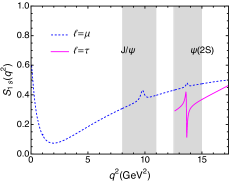
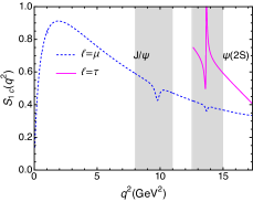
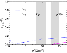
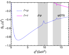
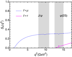
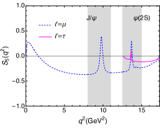
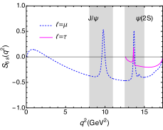
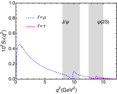
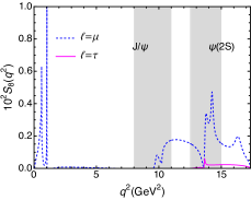
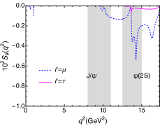
Figure 5: The $q^{2}$ dependence of normalized $CP$-averaged angular coefficients $S_{i}$, where the blue dashed and magenta solid curves are our results for the $\mu$ and $\tau$ modes, respectively.

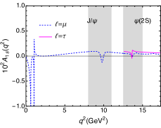
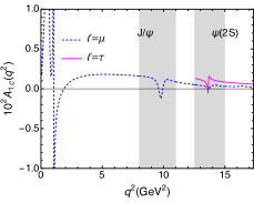
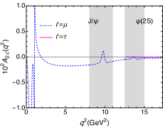
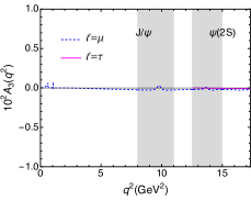
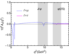
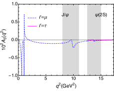
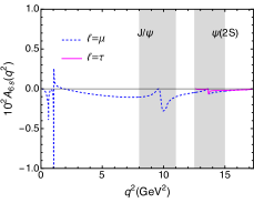
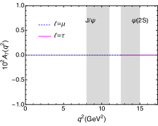
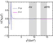
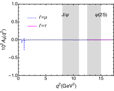
Figure 6: The $q^{2}$ dependence of normalized $CP$ asymmetry angular coefficients $A_{i}$, where the blue dashed and magenta solid curves are our results for the $\mu$ and $\tau$ modes, respectively.

We further evaluate the $CP$-averaged differential branching fractions by using Eqs. (2.21) and (2.22). The $q^{2}$ dependence of the differential branching fractions are shown in Fig. 7, where the red, blue and magenta curves represent the $e$, $\mu$, and $\tau$ modes, respectively. The gray areas also denote the charm loop contributions from the charmonium states $J/\psi$ and $\psi(2S)$. In Table 6, we present our result of the branching fractions and their ratios in different $q^{2}$ bins. In the four $q^{2}$ intervals, i.e., $[1.1,6.0]$, $[6.0,8.0]$, $[11.0,12.5]$, and $[15.0,17.0]\ \text{GeV}^{2}$, the branching fractions of the electron and muon modes can reach up to $10^{-8}$, and the ratio $R^{e\mu}=1$, which is consistent with the SM prediction and reflects the LFU. In the high $q^{2}$ region, that is $[15.0,17.0]\ \text{GeV}^{2}$, the branching fraction of the tau mode is on the order of magnitude of $10^{-9}$. We also obtain the ratio $R^{\tau\mu}=0.384$. In the region of $1.1<q^{2}<6.0~{}\text{GeV}^{2}$, we have the branching fractions as

$$\mathcal{B}(B_{c}\to{D_{s}^{*}}(\to D_{s}\pi){e}^{+}{e}^{-})_{1.1<q^{2}<6.0\text{GeV}^{2}} = 0.624\times 10^{-8},$$

$$\mathcal{B}(B_{c}\to{D_{s}^{*}}(\to D_{s}\pi){\mu}^{+}{\mu}^{-})_{1.1<q^{2}<6.0\text{GeV}^{2}} = 0.622\times 10^{-8}.$$

In addition, combined with the branching fraction $\mathcal{B}(D_{s}^{*}\to{D_{s}}\pi)=5\%$, we have

$$\mathcal{B}(B_{c}\to{D_{s}^{*}}{e}^{+}{e}^{-})_{1.1<q^{2}<6.0\text{GeV}^{2}} = 1.25\times 10^{-7},$$

$$\mathcal{B}(B_{c}\to{D_{s}^{*}}{\mu}^{+}{\mu}^{-})_{1.1<q^{2}<6.0\text{GeV}^{2}} = 1.24\times 10^{-7},$$

which may well be tested by the ongoing LHCb experiment.

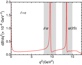
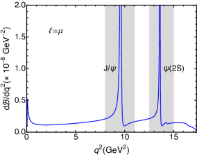
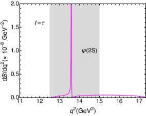
Figure 7: The $q^{2}$ dependence of differential branching fractions $\mathcal{B}(B_{c}\to D_{s}^{*}(\to D_{s}\pi)\ell^{+}\ell^{-})$ [$\ell$=$e$ (left panel), $\mu$ (center panel), and $\tau$ (right panel)], where the red, blue, and magenta curves are our results for the $e$, $\mu$, and $\tau$ modes, respectively.

Table 6: Our results of the branching fractions of $B_{c}\to{D}_{s}^{*}(\to{D}_{s}\pi)\ell^{+}\ell^{-}$ ($\ell$= $e$, $\mu$, $\tau$) (in units of $10^{-8}$) in different $q^{2}$ bins.

$q^{2}$ bins $(\text{GeV}^{2})$	$\mathcal{B}(\ell=e)$	$\mathcal{B}(\ell=\mu)$	$\mathcal{B}(\ell=\tau)$
$[1.1,6.0]$	$0.624$	$0.622$
	$R^{e\mu}=1.00$
$[6.0,8.0]$	$0.356$	$0.355$
	$R^{e\mu}=1.00$
$[11.0,12.5]$	$0.283$	$0.283$
	$R^{e\mu}=1.00$
$[15.0,17.0]$	$0.256$	$0.256$	$0.098$
	$R^{e\mu}=1.00,~{}~{}~{}R^{\tau\mu}=0.384$

We also investigate the physical observables, i.e., the lepton forward-backward asymmetry parameter $A_{FB}$ and the longitudinal (transverse) polarization fractions $F_{L}(F_{T})$. The $q^{2}$ dependence of these observables is presented in Figs. 8 and 9, respectively. Their averaged values in different $q^{2}$ bins, defined by

$$\langle{A}\rangle\big{|}_{q_{\text{min}}^{2}}^{q_{\text{max}}^{2}}=\frac{\int_{q_{\text{min}}^{2}}^{q_{\text{max}}^{2}}A[q^{2}]\Big{(}\frac{d\Gamma}{dq^{2}}+\frac{d\bar{\Gamma}}{dq^{2}}\Big{)}dq^{2}}{\int_{q_{\text{min}}^{2}}^{q_{\text{max}}^{2}}\Big{(}\frac{d\Gamma}{dq^{2}}+\frac{d\bar{\Gamma}}{dq^{2}}\Big{)}dq^{2}},$$ (4.3)

where $A=(A_{FB},\ F_{L},\ F_{T})$, are shown in Table 7.

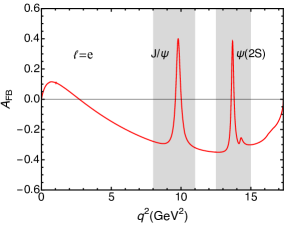
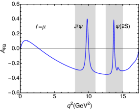
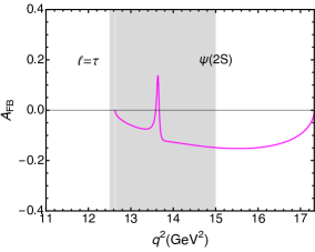
Figure 8: The $q^{2}$ dependence of lepton forward-backward asymmetry parameter $A_{FB}$ in $B_{c}\to D_{s}^{*}(\to D_{s}\pi)\ell^{+}\ell^{-}$ [$\ell$=$e$ (left panel), $\mu$ (center panel), and $\tau$ (right panel)] processes, where the red, the blue, and the magenta curves are our results from the $e$, $\mu$, and $\tau$ modes, respectively.

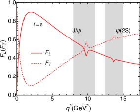
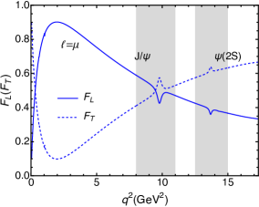
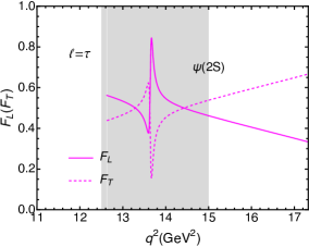
Figure 9: The $q^{2}$ dependence of $D_{s}^{*}$ longitudinal (transverse) polarization fractions $F_{L}(F_{T})$ in $B_{c}\to D_{s}^{*}(\to D_{s}\pi)\ell^{+}\ell^{-}$ [$\ell$=$e$ (left panel), $\mu$ (center panel), and $\tau$ (right panel)] processes, where the red, the blue, and the magenta curves are our results from the $e$, $\mu$, and $\tau$ modes, respectively, and the solid and dashed curves represent the $F_{L}$ and $F_{T}$, respectively.

Table 7: The averaged forward-backward asymmetry $\langle{A_{FB}}\rangle$ and the longitudinal (transverse) polarization fractions $\langle{F_{L}}\rangle(\langle{F_{T}}\rangle)$ in different $q^{2}$ bins.

$q^{2}$ bins $(\text{GeV}^{2})$	$\langle{A_{FB}(\ell=e)}\rangle$	$\langle{A_{FB}(\ell=\mu)}\rangle$	$\langle{A_{FB}(\ell=\tau)}\rangle$
$[1.1,6.0]$	$-0.061$	$-0.061$
$[6.0,8.0]$	$-0.243$	$-0.242$
$[11.0,12.5]$	$-0.340$	$-0.339$
$[15.0,17.0]$	$-0.254$	$-0.254$	$-0.143$
$q^{2}$ bins $(\text{GeV}^{2})$	$\langle{F_{L}(\ell=e)}\rangle$	$\langle{F_{L}(\ell=\mu)}\rangle$	$\langle{F_{L}(\ell=\tau)}\rangle$
$[1.1,6.0]$	$0.815$	$0.817$
$[6.0,8.0]$	$0.637$	$0.638$
$[11.0,12.5]$	$0.446$	$0.446$
$[15.0,17.0]$	$0.352$	$0.352$	$0.410$
$q^{2}$ bins $(\text{GeV}^{2})$	$\langle{F_{T}(\ell=e)}\rangle$	$\langle{F_{T}(\ell=\mu)}\rangle$	$\langle{F_{T}(\ell=\tau)}\rangle$
$[1.1,6.0]$	$0.185$	$0.183$
$[6.0,8.0]$	$0.363$	$0.362$
$[11.0,12.5]$	$0.554$	$0.554$
$[15.0,17.0]$	$0.648$	$0.648$	$0.590$

In addition, we present our results for the $q^{2}$ dependent clean angular observables $P_{1,2,3}$ and $P_{4,5,6,8}^{\prime}$ in Fig. 10. In Ref. LHCb:2013ghj , the LHCb collaboration reported the measurement of the form-factor-independent observables $P^{\prime}_{4,5,6,8}$ of the $B^{0}\to{K^{*0}}\mu^{+}\mu^{-}$ decay. In particular, in the interval of $4.30<q^{2}<8.68$ $\text{GeV}^{2}$, the observable $P_{5}^{\prime}$ shows $3.7\sigma$ discrepancy with the SM prediction Egede:2008uy . After integration over the energy region $1.0<q^{2}<6.0$ $\text{GeV}^{2}$, the discrepancy is determined to be $2.5\sigma$. So we want to investigate these clean angular observables in the rare semileptonic decay of bottom-charmed meson. In order to exclude the charmonium contributions and make it easy to check experimentally, we also present the averaged values of these observables in different $q^{2}$ intervals in Table 8. The averaged value in a $q^{2}$ bin is defined by Eq. (4.3).

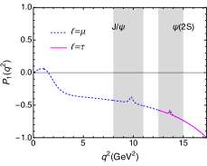
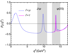
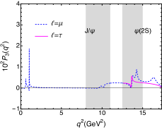
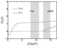
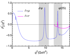
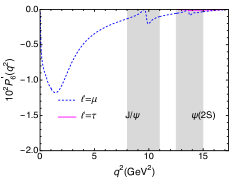
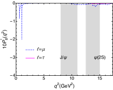
Figure 10: The $q^{2}$ dependence of the clean angular observables $P_{1,2,3}$ and $P_{4,5,6,8}^{\prime}$, where the blue dashed and magenta solid curves represent our results for the $\mu$ and $\tau$ modes, respectively.

Table 8: The averaged values of the clean angular observables $P_{1,2,3}$ and $P^{\prime}_{4,5,6,8}$ in different $q^{2}$ bins.

$q^{2}$ bins $(\text{GeV}^{2})$	$\langle{P_{1}(\ell=e)}\rangle$	$\langle{P_{1}(\ell=\mu)}\rangle$	$\langle{P_{1}(\ell=\tau)}\rangle$	$q^{2}$ bins $(\text{GeV}^{2})$	$\langle{P_{4}^{\prime}(\ell=e)}\rangle$	$\langle{P_{4}^{\prime}(\ell=\mu)}\rangle$	$\langle{P_{4}^{\prime}(\ell=\tau)}\rangle$
$[1.1,6.0]$	$-0.281$	$-0.281$		$[1.1,6.0]$	$0.908$	$0.898$
$[6.0,8.0]$	$-0.408$	$-0.408$		$[6.0,8.0]$	$1.177$	$1.169$
$[11.0,12.5]$	$-0.543$	$-0.543$		$[11.0,12.5]$	$1.240$	$1.236$
$[15.0,17.0]$	$-0.822$	$-0.822$	$-0.826$	$[15.0,17.0]$	$1.350$	$1.347$	$0.561$
$q^{2}$ bins $(\text{GeV}^{2})$	$\langle{P_{2}(\ell=e)}\rangle$	$\langle{P_{2}(\ell=\mu)}\rangle$	$\langle{P_{2}(\ell=\tau)}\rangle$	$q^{2}$ bins $(\text{GeV}^{2})$	$\langle{P_{5}^{\prime}(\ell=e)}\rangle$	$\langle{P_{5}^{\prime}(\ell=\mu)}\rangle$	$\langle{P_{5}^{\prime}(\ell=\tau)}\rangle$
$[1.1,6.0]$	$-0.125$	$-0.125$		$[1.1,6.0]$	$-0.540$	$-0.534$
$[6.0,8.0]$	$-0.446$	$-0.446$		$[6.0,8.0]$	$-0.766$	$-0.761$
$[11.0,12.5]$	$-0.409$	$-0.409$		$[11.0,12.5]$	$-0.664$	$-0.662$
$[15.0,17.0]$	$-0.262$	$-0.262$	$-0.269$	$[15.0,17.0]$	$-0.390$	$-0.390$	$-0.163$
$q^{2}$ bins $(\text{GeV}^{2})$	$10^{3}\langle{P_{3}(\ell=e)}\rangle$	$10^{3}\langle{P_{3}(\ell=\mu)}\rangle$	$10^{3}\langle{P_{3}(\ell=\tau)}\rangle$	$q^{2}$ bins $(\text{GeV}^{2})$	$10^{3}\langle{P_{6}^{\prime}(\ell=e)}\rangle$	$10^{3}\langle{P_{6}^{\prime}(\ell=\mu)}\rangle$	$10^{3}\langle{P_{6}^{\prime}(\ell=\tau)}\rangle$
$[1.1,6.0]$	$0.184$	$0.184$		$[1.1,6.0]$	$-6.440$	$-6.320$
$[6.0,8.0]$	$0.007$	$0.007$		$[6.0,8.0]$	$-1.868$	$-1.856$
$[11.0,12.5]$	$2.421$	$2.421$		$[11.0,12.5]$	$-0.771$	$-0.769$
$[15.0,17.0]$	$3.442$	$3.442$	$2.008$	$[15.0,17.0]$	$-0.188$	$-0.188$	$-0.070$
				$q^{2}$ bins $(\text{GeV}^{2})$	$10^{3}\langle{P_{8}^{\prime}(\ell=e)}\rangle$	$10^{3}\langle{P_{8}^{\prime}(\ell=\mu)}\rangle$	$10^{3}\langle{P_{8}^{\prime}(\ell=\tau)}\rangle$
				$[1.1,6.0]$	$-1.196$	$-1.164$
				$[6.0,8.0]$	$-0.029$	$-0.029$
				$[11.0,12.5]$	$-7.054$	$-7.030$
				$[15.0,17.0]$	$-6.147$	$-6.137$	$-1.467$

In general, this quasi-four-body decay provides a set of physical observables to study the corresponding weak interaction, and in particular the ratios of the branching fractions $R^{e\mu}$ and $R^{\tau\mu}$, as well as the clean angular coefficients $P_{i}$ and $P_{j}^{\prime}$, can be helpful to search for the NP effects beyond the SM. We call for the ongoing LHCb experiment to search for this process and to measure the corresponding physical observables.

V Summary

In this work, we have studied the $B_{c}\to{D_{s}^{*}}$ transition form factors deduced by the (axial)vector and (pseudo)tensor currents, and, in the future, investigate the angular distributions of the quasi-four-body processes $B_{c}\to{D}_{s}^{*}(\to{D}_{s}\pi)\ell^{+}\ell^{-}$ ($\ell$=$e$, $\mu$, $\tau$).

To describe the weak process, the relevant seven independent form factors are calculated by utilizing the covariant LFQM approach. The concerned meson wave functions are adopted as the numerical wave functions, which are extracted from the solution of the modified GI model. This treatment avoids the $\beta$ dependence and thus reduces the corresponding uncertainty. Our results of form factors are compared with other approaches. In particular, for the (pseudo)tensor currents deduced form factors $T_{1,2,3}(q^{2}=0)$, our results agree with the pQCD prediction. More theoretical works, especially the LQCD and QCD sum rule (or light-cone sum rule) calculation, are highly appreciated to test our result and to refine the corresponding topic.

With the obtained form factors, the rare semileptonic decays $B_{c}\to{D}_{s}^{*}(\to{D}_{s}\pi)\ell^{+}\ell^{-}$ are studied. Not only the branching fractions, the lepton-side forward-backward asymmetry parameter $A_{FB}$, and the longitudinal and transverse polarization fractions $F_{L}$ and $F_{T}$, but also the angular coefficients $S_{i}$ and $A_{i}$ are investigated. Numerically, the concerned cascade decays with $e$ or $\mu$ final states are around $10^{-8}$, which need to be tested by other approaches and ongoing experiments. Moreover, the $A_{FB}$ and $F_{L(T)}$ are important physical observables, and they are also feasible observables in the future LHCb experiment, so we look forward to the experimental results. In addition, the ratios of the branching fractions are also calculated to validate whether or not the LFU violated. Furthermore, the clean coefficient observables $P_{i}$ and $P_{j}^{\prime}$ are presented, which reduce the uncertainty from the form factors and can be a possible signal to search for the NP effects. Since these observations are largely free of form factor uncertainties in the large-recoiled limit, and are feasible to measure experimentally, we strongly encourage our experimental colleagues to measure them.

Overall, in this work we have systematically studied the angular distribution of $B_{c}\to{D_{s}^{*}}(\to{D_{s}}\pi)\ell^{+}\ell^{-}$ ($\ell$= $e$, $\mu$, $\tau$) with the form factors obtained by the covariant LFQM. We live in the hope that with the completion of the LHCb experiment prepared for the run 3 and run 4 of the LHC and the improvement of the experimental capabilities, this rare semileptonic process can be discovered and we expect that the predicted physical observables can be tested.

Appendix A The weak transition matrix elements deduced by axial-vector and (pseudo)tensor currents

In this Appendix, we present the concerned expressions of the weak transition matrix elements deduced by axial-vector current , and (pseudo)tensor currents. The expression of the axial-vector current matrix element is

$$\begin{split}S_{\mu\nu}^{A}=&\text{Tr}\Big{[}\Big{(}\gamma_{\nu}-\frac{(p_{1}^{\prime\prime}-p_{2})_{\nu}}{W_{V}^{\prime\prime}}\Big{)}(\not{p}_{1}^{\prime\prime}+m_{1}^{\prime\prime})\gamma_{\mu}\gamma_{5}(\not{p}_{1}^{\prime}+m_{1}^{\prime})\gamma_{5}(-\not{p}_{2}+m_{2})\Big{]}\\ =&-2g_{\mu\nu}\bigg{[}m_{2}(q^{2}-N_{1}^{\prime}-N_{1}^{\prime\prime}-m_{1}^{\prime 2}-m_{1}^{\prime\prime 2})-m_{1}^{\prime}(M^{\prime\prime 2}-N_{1}^{\prime\prime}-N_{2}-m_{1}^{\prime\prime 2}-m_{2}^{2})\\ &-m_{1}^{\prime\prime}(M^{\prime 2}-N_{1}^{\prime}-N_{2}-m_{1}^{\prime 2}-m_{2}^{2})-2m_{1}^{\prime}m_{1}^{\prime\prime}m_{2}\bigg{]}-8p_{1\mu}^{\prime}p_{1\nu}^{\prime}(m_{2}-m_{1}^{\prime})\\ &+2m_{1}^{\prime}(P_{\mu}q_{\nu}+P_{\nu}q_{\mu}+2q_{\mu}q_{\nu})-2p_{1\mu}^{\prime}P_{\nu}(m_{1}^{\prime}-m_{1}^{\prime\prime})-2p_{1\nu}^{\prime}P_{\mu}(m_{1}^{\prime}+m_{1}^{\prime\prime})\\ &-2p_{1\mu}^{\prime}q_{\nu}(3m_{1}^{\prime}-m_{1}^{\prime\prime}-2m_{2})-2p_{1\nu}^{\prime}q_{\mu}(3m_{1}^{\prime}+m_{1}^{\prime\prime}-2m_{2})\\ &-\frac{1}{2W_{V}^{\prime\prime}}\bigg{[}2p_{1\mu}^{\prime}(M^{\prime 2}+M^{\prime\prime 2}-q^{2}-2N_{2}+2(m_{1}^{\prime}-m_{2})(m_{1}^{\prime\prime}+m_{2}))\\ &+q_{\mu}(q^{2}-2M^{\prime 2}+N_{1}^{\prime}-N_{1}^{\prime\prime}+2N_{2}-(m_{1}+m_{1}^{\prime\prime})^{2}+2(m_{1}^{\prime}-m_{2})^{2})\\ &+P_{\mu}(q^{2}-N_{1}^{\prime}-N_{1}^{\prime\prime}-(m_{1}^{\prime}+m_{1}^{\prime\prime})^{2})\bigg{]}(4p_{1\nu}^{\prime}-3q_{\nu}-P_{\nu}),\end{split}$$ (A.1)

and the expression of the (pseudo)tensor current matrix element is

$$S_{\mu\nu}^{T+T5}=\text{Tr}\Big{[}\Big{(}\gamma_{\nu}-\frac{(p_{1}^{\prime\prime}-p_{2})_{\nu}}{W_{V}^{\prime\prime}}\Big{)}(\not{p}_{1}^{\prime\prime}+m_{1}^{\prime\prime})i\sigma_{\mu\delta}(1+\gamma_{5})q^{\delta}(\not{p}_{1}^{\prime}+m_{1}^{\prime})\gamma_{5}(-\not{p}_{2}+m_{2})\Big{]}.$$ (A.2)

By using the identity $2\sigma_{\mu\delta}\gamma_{5}=-i\epsilon_{\mu\delta\alpha\beta}\sigma^{\alpha\beta}$, the matrix element $S_{\mu\nu}^{T+T5}$ can be decomposed into

$$S_{\mu\nu}^{T+T5}=iq^{\delta}S_{\mu\nu\delta}+\frac{1}{2}\epsilon_{\mu\delta\alpha\beta}q^{\delta}S_{\nu}^{\alpha\beta},$$ (A.3)

where $iq^{\delta}S_{\mu\nu\delta}$ and $\frac{1}{2}\epsilon_{\mu\delta\alpha\beta}q^{\delta}S_{\nu}^{\alpha\beta}$ are expressed as

$$\begin{split}iq^{\delta}S_{\mu\nu\delta}=&\text{Tr}\Big{[}\Big{(}\gamma_{\nu}-\frac{(p_{1}^{\prime\prime}-p_{2})_{\nu}}{W_{V}^{\prime\prime}}\Big{)}(\not{p}_{1}^{\prime\prime}+m_{1}^{\prime\prime})i\sigma_{\mu\delta}q^{\delta}(\not{p}_{1}^{\prime}+m_{1}^{\prime})\gamma_{5}(-\not{p}_{2}+m_{2})\Big{]}\\ =&i\epsilon_{\mu\nu\alpha\beta}P^{\alpha}p_{1}^{\beta}\big{(}m_{1}^{\prime 2}-m_{1}^{\prime\prime 2}+N_{1}^{\prime}-N_{1}^{\prime\prime}\big{)}-\frac{i}{2}\epsilon_{\mu\nu\alpha\beta}P^{\alpha}q^{\beta}\big{(}m_{1}^{\prime 2}+4m_{1}^{\prime}m_{1}^{\prime\prime}-m_{1}^{\prime\prime 2}+N_{1}^{\prime}-N_{1}^{\prime\prime}+q^{2}\big{)}\\ &-i\epsilon_{\mu\nu\alpha\beta}p_{1}^{\alpha}q^{\beta}\big{(}M^{\prime 2}-m_{1}^{\prime 2}+4m_{2}(m_{1}^{\prime}+m_{1}^{\prime\prime})-4m_{1}^{\prime}m_{1}^{\prime\prime}-m_{1}^{\prime\prime 2}-2m_{2}^{2}+M^{\prime\prime 2}-N_{1}^{\prime}-N_{1}^{\prime\prime}-2N_{2}-q^{2}\big{)}\\ &+i\epsilon_{\mu\alpha\beta\gamma}P^{\alpha}p_{1}^{\beta}q^{\gamma}P_{\nu}\big{(}\frac{m_{1}^{\prime}+m_{1}^{\prime\prime}}{W_{V}^{\prime\prime}}\big{)}+i\epsilon_{\mu\alpha\beta\gamma}P^{\alpha}p_{1}^{\beta}q^{\gamma}p_{1\nu}\bigg{(}2-\frac{4(m_{1}^{\prime}+m_{1}^{\prime\prime})}{W_{V}^{\prime\prime}}\bigg{)}+i\epsilon_{\mu\alpha\beta\gamma}P^{\alpha}p_{1}^{\beta}q^{\gamma}q_{\nu}\bigg{(}\frac{3(m_{1}^{\prime}+m_{1}^{\prime\prime})}{W_{V}^{\prime\prime}}-1\bigg{)}\\ &-i\epsilon_{\nu\alpha\beta\gamma}P^{\alpha}p_{1}^{\beta}q^{\gamma}q_{\mu}+2i\epsilon_{\nu\alpha\beta\gamma}P^{\alpha}p_{1}^{\beta}q^{\gamma}p_{1\mu},\end{split}$$ (A.4)

$$\begin{split}\frac{1}{2}\epsilon_{\mu\delta\alpha\beta}q^{\delta}S_{\nu}^{\alpha\beta}=&\text{Tr}\Big{[}\Big{(}\gamma_{\nu}-\frac{(p_{1}^{\prime\prime}-p_{2})_{\nu}}{W_{V}^{\prime\prime}}\Big{)}(\not{p}_{1}^{\prime\prime}+m_{1}^{\prime\prime})\frac{1}{2}\sigma^{\alpha\beta}\epsilon_{\mu\delta\alpha\beta}q^{\delta}(\not{p}_{1}^{\prime}+m_{1}^{\prime})\gamma_{5}(-\not{p}_{2}+m_{2})\Big{]}\\ =&-2ig_{\mu\nu}\big{\{}M^{\prime 2}[m_{1}^{\prime\prime}(m_{1}^{\prime}-m_{1}^{\prime\prime})-N_{1}^{\prime\prime}]+m_{1}^{\prime 3}(m_{2}-m_{1}^{\prime\prime})+m_{1}^{\prime 2}(m_{2}(m_{1}^{\prime\prime}-m_{2})+M^{\prime\prime 2}-N_{2})\\ &+m_{1}^{\prime}(m_{1}^{\prime\prime 3}-m_{1}^{\prime\prime 2}m_{2}-m_{1}^{\prime\prime}(M^{\prime\prime 2}+N_{1}^{\prime}-N_{1}^{\prime\prime})+m_{2}(N_{1}^{\prime}-N_{1}^{\prime\prime}-q^{2}))-m_{1}^{\prime\prime 3}m_{2}+m_{1}^{\prime\prime 2}m_{2}^{2}\\ &+m_{1}^{\prime\prime 2}N_{2}+m_{1}^{\prime\prime}m_{2}N_{1}^{\prime}-m_{1}^{\prime\prime}m_{2}N_{1}^{\prime\prime}+m_{1}^{\prime\prime}m_{2}q^{2}-m_{2}^{2}N_{1}^{\prime}+m_{2}^{2}N_{1}^{\prime\prime}+M^{\prime\prime 2}N_{1}^{\prime}-N_{1}^{\prime}N_{2}+N_{1}^{\prime\prime}N_{2}\big{\}}\\ &+iP_{\mu}P_{\nu}\Big{\{}\frac{(m_{1}^{\prime}+m_{1}^{\prime\prime})(m_{1}^{\prime 2}-m_{1}^{\prime\prime 2}+N_{1}^{\prime}-N_{1}^{\prime\prime})+q^{2}(m_{1}^{\prime\prime}-m_{1}^{\prime})}{2W_{V}^{\prime\prime}}\Big{\}}\\ &+iq_{\mu}q_{\nu}\Big{\{}-2M^{\prime 2}-m_{1}^{\prime 2}+2m_{1}^{\prime}m_{1}^{\prime\prime}-4m_{1}^{\prime}m_{2}+m_{1}^{\prime\prime 2}+2m_{2}^{2}-N_{1}^{\prime}+N_{1}^{\prime\prime}+2N_{2}-q^{2}\\ &+\frac{3}{2W_{V}^{\prime\prime}}\Big{[}2M^{\prime 2}m_{1}^{\prime}-m_{1}^{\prime 3}+m_{1}^{\prime 2}(m_{1}^{\prime\prime}+2m_{2})+m_{1}^{\prime}(m_{1}^{\prime\prime 2}-2M^{\prime\prime 2}-N_{1}^{\prime}+N_{1}^{\prime\prime}-q^{2})\\ &-(m_{1}^{\prime\prime}+2m_{2})(m_{1}^{\prime\prime 2}-N_{1}^{\prime}+N_{1}^{\prime\prime}-q^{2})\Big{]}\Big{\}}\\ &+ip_{1\mu}p_{1\nu}\Big{\{}-4M^{\prime 2}+4M^{\prime\prime 2}-4q^{2}+\frac{4}{W_{V}^{\prime\prime}}\Big{[}(M^{\prime 2}-M^{\prime\prime 2})(m_{1}^{\prime}+m_{1}^{\prime\prime})+q^{2}(-m_{1}^{\prime}+m_{1}^{\prime\prime}+2m_{2})\Big{]}\Big{\}}\\ &+iP_{\mu}p_{1\nu}\Big{\{}2m_{1}^{\prime 2}-2m_{1}^{\prime\prime 2}+2N_{1}^{\prime}-2N_{1}^{\prime\prime}+\frac{2}{W_{V}^{\prime\prime}}\Big{[}q^{2}(m_{1}^{\prime}-m_{1}^{\prime\prime})-(m_{1}^{\prime}+m_{1}^{\prime\prime})(m_{1}^{\prime 2}-m_{1}^{\prime\prime 2}+N_{1}^{\prime}-N_{1}^{\prime\prime})\Big{]}\Big{\}}\\ &+iP_{\nu}p_{1\mu}\Big{\{}2q^{2}+\frac{1}{W_{V}^{\prime\prime}}\Big{[}q^{2}(m_{1}^{\prime}-m_{1}^{\prime\prime}-2m_{2})-(M^{\prime 2}-M^{\prime\prime 2})(m_{1}^{\prime}+m_{1}^{\prime\prime})\Big{]}\Big{\}}\\ &+iP_{\mu}q_{\nu}\Big{\{}-2m_{1}^{\prime 2}+2m_{1}^{\prime}m_{1}^{\prime\prime}-2N_{1}^{\prime}+\frac{3}{2W_{V}^{\prime\prime}}\Big{[}(m_{1}^{\prime}+m_{1}^{\prime\prime})(m_{1}^{\prime 2}-m_{1}^{\prime\prime 2}+N_{1}^{\prime}-N_{1}^{\prime\prime})+q^{2}(m_{1}^{\prime\prime}-m_{1}^{\prime})\Big{]}\Big{\}}\\ &+iP_{\nu}q_{\mu}\Big{\{}-m_{1}^{\prime 2}+m_{1}^{\prime\prime 2}-N_{1}^{\prime}+N_{1}^{\prime\prime}-q^{2}+\frac{1}{2W_{V}^{\prime\prime}}\Big{[}2M^{\prime 2}m_{1}^{\prime}-m_{1}^{\prime 3}+m_{1}^{\prime 2}(m_{1}^{\prime\prime}+2m_{2})\\ &+m_{1}^{\prime}(m_{1}^{\prime\prime 2}-2M^{\prime\prime 2}-N_{1}^{\prime}+N_{1}^{\prime\prime}-q^{2})-(m_{1}^{\prime\prime}+2m_{2})(m_{1}^{\prime\prime 2}-N_{1}^{\prime}+N_{1}^{\prime\prime}-q^{2})\Big{]}\Big{\}}\\ &+ip_{1\mu}q_{\nu}\Big{\{}4M^{\prime 2}-4m_{1}^{\prime}m_{1}^{\prime\prime}+4m_{1}^{\prime}m_{2}+4m_{1}^{\prime\prime}m_{2}-4m_{2}^{2}-4N_{2}+2q^{2}\\ &+\frac{3}{W_{V}^{\prime\prime}}\Big{[}q^{2}(m_{1}^{\prime}-m_{1}^{\prime\prime}-2m_{2})-(M^{\prime 2}-M^{\prime\prime 2})(m_{1}^{\prime}+m_{1}^{\prime\prime})\Big{]}\Big{\}}\\ &+ip_{1\nu}q_{\mu}\Big{\{}2M^{\prime 2}+2m_{1}^{\prime 2}-2m_{1}^{\prime\prime 2}-2M^{\prime\prime 2}+2N_{1}^{\prime}-2N_{1}^{\prime\prime}+2q^{2}-\frac{2}{W_{V}^{\prime\prime}}\Big{[}2M^{\prime 2}m_{1}^{\prime}-m_{1}^{\prime 3}+m_{1}^{\prime 2}(m_{1}^{\prime\prime}+2m_{2})\\ &+m_{1}^{\prime}(m_{1}^{\prime\prime 2}-2M^{\prime\prime 2}-N_{1}^{\prime}+N_{1}^{\prime\prime}-q^{2})-(m_{1}^{\prime\prime}+2m_{2})(m_{1}^{\prime\prime 2}-N_{1}^{\prime}+N_{1}^{\prime\prime}-q^{2})\Big{]}\Big{\}},\end{split}$$ (A.5)

respectively.

References

- (1) W. Altmannshofer and D. M. Straub, New physics in transitions after LHC run 1, Eur. Phys. J. C 75 (2015) no.8, 382.
- (2) S. Descotes-Genon, L. Hofer, J. Matias and J. Virto, Global analysis of anomalies, JHEP 06 (2016), 092.
- (3) N. R. Singh Chundawat, New physics in : A model independent analysis, Phys. Rev. D 107 (2023) no.5, 055004.
- (4) T. Skwarnicki [CLEO], Update on and from CLEO,
- (5) T. Affolder et al. [CDF], Search for the flavor-changing neutral current decays and , Phys. Rev. Lett. 83 (1999), 3378-3383.
- (6) B. Aubert et al. [BaBar], Search for and , [arXiv:hep-ex/0008059 [hep-ex]].
- (7) K. Abe et al. [Belle], Observation of the decay , Phys. Rev. Lett. 88 (2002), 021801.
- (8) A. Ishikawa et al. [Belle], Observation of , Phys. Rev. Lett. 91 (2003), 261601.
- (9) J. T. Wei et al. [Belle], Measurement of the Differential Branching Fraction and Forward-Backward Asymmetry for , Phys. Rev. Lett. 103 (2009), 171801.
- (10) S. Wehle et al. [Belle], Lepton-Flavor-Dependent Angular Analysis of , Phys. Rev. Lett. 118 (2017) no.11, 111801.
- (11) S. Choudhury et al. [BELLE], Test of lepton flavor universality and search for lepton flavor violation in decays, JHEP 03 (2021), 105.
- (12) A. Abdesselam et al. [Belle], Test of Lepton-Flavor Universality in Decays at Belle, Phys. Rev. Lett. 126 (2021) no.16, 161801.
- (13) B. Aubert et al. [BaBar], Evidence for the rare decay and measurement of the branching fraction, Phys. Rev. Lett. 91 (2003), 221802.
- (14) B. Aubert et al. [BaBar], Direct CP, Lepton Flavor and Isospin Asymmetries in the Decays , Phys. Rev. Lett. 102 (2009), 091803.
- (15) J. P. Lees et al. [BaBar], Measurement of Branching Fractions and Rate Asymmetries in the Rare Decays , Phys. Rev. D 86 (2012), 032012.
- (16) T. Aaltonen et al. [CDF], Observation of the Baryonic Flavor-Changing Neutral Current Decay , Phys. Rev. Lett. 107 (2011), 201802.
- (17) V. Khachatryan et al. [CMS], Angular analysis of the decay from pp collisions at TeV, Phys. Lett. B 753 (2016), 424-448.
- (18) R. Aaij et al. [LHCb], Differential branching fraction and angular analysis of the decay, JHEP 02 (2013), 105.
- (19) R. Aaij et al. [LHCb], Test of lepton universality using decays, Phys. Rev. Lett. 113 (2014), 151601.
- (20) R. Aaij et al. [LHCb], Measurements of the S-wave fraction in decays and the differential branching fraction, JHEP 11 (2016), 047 [erratum: JHEP 04 (2017), 142].
- (21) R. Aaij et al. [LHCb], Test of lepton universality with decays, JHEP 08 (2017), 055.
- (22) R. Aaij et al. [LHCb], Test of lepton universality in beauty-quark decays, Nature Phys. 18 (2022) no.3, 277-282.
- (23) R. Aaij et al. [LHCb], Measurement of Form-Factor-Independent Observables in the Decay , Phys. Rev. Lett. 111 (2013), 191801.
- (24) U. Egede, T. Hurth, J. Matias, M. Ramon and W. Reece, New observables in the decay mode , JHEP 11 (2008), 032.
- (25) M. Bordone, G. Isidori and A. Pattori, On the Standard Model predictions for and , Eur. Phys. J. C 76 (2016) no.8, 440.
- (26) D. Acosta et al. [CDF], Search for the Decay in Collisions at = 1.8-TeV, Phys. Rev. D 65 (2002), 111101.
- (27) T. Aaltonen et al. [CDF], Search for the Rare Decays , , and at CDF, Phys. Rev. D 79 (2009), 011104.
- (28) V. M. Abazov et al. [D0], Search for the rare decay with the D0 detector, Phys. Rev. D 74 (2006), 031107.
- (29) T. Aaltonen et al. [CDF], Measurement of the Forward-Backward Asymmetry in the Decay and First Observation of the Decay, Phys. Rev. Lett. 106 (2011), 161801.
- (30) R. Aaij et al. [LHCb], Differential branching fraction and angular analysis of the decay , JHEP 07 (2013), 084.
- (31) R. Aaij et al. [LHCb], Angular analysis and differential branching fraction of the decay , JHEP 09 (2015), 179.
- (32) R. Aaij et al. [LHCb], Branching Fraction Measurements of the Rare and Decays, Phys. Rev. Lett. 127 (2021) no.15, 151801.
- (33) T. V. Dong et al. [Belle], Search for the decay at the Belle experiment, Phys. Rev. D 108 (2023) no.1, L011102.
- (34) C. Bouchard et al. [HPQCD], Rare decay form factors from lattice QCD, Phys. Rev. D 88 (2013) no.5, 054509 [erratum: Phys. Rev. D 88 (2013) no.7, 079901].
- (35) R. R. Horgan, Z. Liu, S. Meinel and M. Wingate, Lattice QCD calculation of form factors describing the rare decays and , Phys. Rev. D 89 (2014) no.9, 094501.
- (36) J. A. Bailey, A. Bazavov, C. Bernard, C. M. Bouchard, C. DeTar, D. Du, A. X. El-Khadra, J. Foley, E. D. Freeland and E. Gámiz, et al. Decay Form Factors from Three-Flavor Lattice QCD, Phys. Rev. D 93 (2016) no.2, 025026.
- (37) P. Ball and R. Zwicky, decay form-factors from light-cone sum rules revisited, Phys. Rev. D 71 (2005), 014029.
- (38) P. Ball and R. Zwicky, New results on decay formfactors from light-cone sum rules, Phys. Rev. D 71 (2005), 014015.
- (39) Y. L. Wu, M. Zhong and Y. B. Zuo, Transition Form Factors and Decay Rates with Extraction of the CKM parameters , , , Int. J. Mod. Phys. A 21 (2006), 6125-6172.
- (40) M. Bartsch, M. Beylich, G. Buchalla and D. N. Gao, Precision Flavour Physics with and , JHEP 11 (2009), 011.
- (41) A. Bharucha, D. M. Straub and R. Zwicky, in the Standard Model from light-cone sum rules, JHEP 08 (2016), 098.
- (42) W. Cheng, X. G. Wu and H. B. Fu, Reconsideration of the transition form factors within the QCD light-cone sum rules, Phys. Rev. D 95 (2017) no.9, 094023.
- (43) J. Gao, C. D. Lü, Y. L. Shen, Y. M. Wang and Y. B. Wei, Precision calculations of form factors from soft-collinear effective theory sum rules on the light-cone, Phys. Rev. D 101 (2020) no.7, 074035.
- (44) Y. M. Wang and Y. L. Shen, QCD corrections to form factors from light-cone sum rules, Nucl. Phys. B 898 (2015), 563-604.
- (45) Y. M. Wang, Y. B. Wei, Y. L. Shen and C. D. Lü, Perturbative corrections to form factors in QCD, JHEP 06 (2017), 062.
- (46) C. D. Lü, Y. L. Shen, Y. M. Wang and Y. B. Wei, QCD calculations of form factors with higher-twist corrections, JHEP 01 (2019), 024.
- (47) J. Gao, T. Huber, Y. Ji, C. Wang, Y. M. Wang and Y. B. Wei, form factors beyond leading power and extraction of and , JHEP 05 (2022), 024.
- (48) B. Y. Cui, Y. K. Huang, Y. L. Shen, C. Wang and Y. M. Wang, Precision calculations of decay form factors in soft-collinear effective theory, JHEP 03 (2023), 140.
- (49) B. Y. Cui, Y. K. Huang, Y. M. Wang and X. C. Zhao, Shedding New Light on and from Semileptonic Decays, [arXiv:2301.12391 [hep-ph]].
- (50) C. Bobeth, G. Hiller and G. Piranishvili, CP Asymmetries in bar and Untagged , Decays at NLO, JHEP 07 (2008), 106.
- (51) R. H. Li, C. D. Lü and W. Wang, Transition form factors of decays into -wave axial-vector mesons in the perturbative QCD approach, Phys. Rev. D 79 (2009), 034014.
- (52) W. Wang, R. H. Li and C. D. Lü, Radiative charmless and decays in pQCD approach, [arXiv:0711.0432 [hep-ph]].
- (53) R. H. Li, C. D. Lü and W. Wang, Branching Ratios, Forward-backward Asymmetry and Angular Distributions of Decays, Phys. Rev. D 79 (2009), 094024.
- (54) W. F. Wang and Z. J. Xiao, The semileptonic decays in the perturbative QCD approach beyond the leading-order, Phys. Rev. D 86 (2012), 114025.
- (55) W. F. Wang, Y. Y. Fan, M. Liu and Z. J. Xiao, Semileptonic decays in the perturbative QCD approach beyond the leading order, Phys. Rev. D 87 (2013) no.9, 097501.
- (56) Z. J. Xiao and X. Liu, The two-body hadronic decays of meson in the perturbative QCD approach: A short review, Chin. Sci. Bull. 59 (2014), 3748-3759.
- (57) S. P. Jin, X. Q. Hu and Z. J. Xiao, Study of decays in the PQCD factorization approach with lattice QCD input, Phys. Rev. D 102 (2020) no.1, 013001.
- (58) S. P. Jin and Z. J. Xiao, Study of Decays in the PQCD Factorization Approach with Lattice QCD Input, Adv. High Energy Phys. 2021 (2021), 3840623.
- (59) A. Deandrea and A. D. Polosa, The Exclusive process in a constituent quark model, Phys. Rev. D 64 (2001), 074012.
- (60) C. Q. Geng and C. C. Liu, Study of (, , decays, J. Phys. G 29 (2003), 1103-1118.
- (61) C. H. Chen, C. Q. Geng and W. Wang, Z-mediated charge and CP asymmetries and FCNCs in processes, JHEP 11 (2010), 089.
- (62) R. H. Li, C. D. Lü and W. Wang, Branching ratios, forward-backward asymmetries and angular distributions of in the standard model and new physics scenarios, Phys. Rev. D 83 (2011), 034034.
- (63) S. Dubnička, A. Z. Dubničková, A. Issadykov, M. A. Ivanov, A. Liptaj and S. K. Sakhiyev, Decay in covariant quark model, Phys. Rev. D 93 (2016) no.9, 094022.
- (64) N. R. Soni, A. Issadykov, A. N. Gadaria, J. J. Patel and J. N. Pandya, Rare decays in covariant confined quark model, Eur. Phys. J. A 58 (2022) no.3, 39.
- (65) A. Issadykov, Decay in Covariant Confined Quark Model, Phys. Part. Nucl. Lett. 19 (2022) no.5, 460-462.
- (66) C. D. Lü and W. Wang, Analysis of in the higher kaon resonance region, Phys. Rev. D 85 (2012), 034014.
- (67) M. Ahmady, S. Keller, M. Thibodeau and R. Sandapen, Reexamination of the rare decay using holographic light-front QCD, Phys. Rev. D 100 (2019) no.11, 113005.
- (68) N. Rajeev, N. Sahoo and R. Dutta, Angular analysis of decays as a probe to lepton flavor universality violation, Phys. Rev. D 103 (2021) no.9, 095007.
- (69) S. P. Li, X. Q. Li, Y. D. Yang and X. Zhang, and neutrino mass in the 2HDM-III with right-handed neutrinos, JHEP 09 (2018), 149.
- (70) B. Barman, D. Borah, L. Mukherjee and S. Nandi, Correlating the anomalous results in decays with inert Higgs doublet dark matter and muon , Phys. Rev. D 100 (2019) no.11, 115010.
- (71) L. Delle Rose, S. Khalil, S. J. D. King and S. Moretti, and in an Aligned 2HDM with Right-Handed Neutrinos, Phys. Rev. D 101 (2020) no.11, 115009.
- (72) A. Ordell, R. Pasechnik, H. Serôdio and F. Nottensteiner, Classification of anomaly-free 2HDMs with a gauged symmetry, Phys. Rev. D 100 (2019) no.11, 115038.
- (73) C. Marzo, L. Marzola and M. Raidal, Common explanation to the , and anomalies in a 3HDM+ and connections to neutrino physics, Phys. Rev. D 100 (2019) no.5, 055031.
- (74) S. Iguro and Y. Omura, Status of the semileptonic decays and muon g-2 in general 2HDMs with right-handed neutrinos, JHEP 05 (2018), 173.
- (75) S. Iguro, Conclusive probe of the charged Higgs solution of and discrepancies, Phys. Rev. D 107 (2023) no.9, 095004.
- (76) M. J. Aslam, C. D. Lü and Y. M. Wang, decays in supersymmetric theories, Phys. Rev. D 79 (2009), 074007.
- (77) S. Trifinopoulos, -physics anomalies: The bridge between R-parity violating supersymmetry and flavored dark matter, Phys. Rev. D 100 (2019) no.11, 115022.
- (78) A. Shaw, Looking for in a nonminimal universal extra dimensional model, Phys. Rev. D 99 (2019) no.11, 115030.
- (79) W. Altmannshofer, S. Gori, M. Pospelov and I. Yavin, Quark flavor transitions in models, Phys. Rev. D 89 (2014), 095033.
- (80) B. Bhattacharya, A. Datta, D. London and S. Shivashankara, Simultaneous Explanation of the and Puzzles, Phys. Lett. B 742 (2015), 370-374.
- (81) A. Crivellin, G. D’Ambrosio and J. Heeck, Addressing the LHC flavor anomalies with horizontal gauge symmetries, Phys. Rev. D 91 (2015) no.7, 075006.
- (82) A. Celis, J. Fuentes-Martin, M. Jung and H. Serodio, Family nonuniversal models with protected flavor-changing interactions, Phys. Rev. D 92 (2015) no.1, 015007.
- (83) A. Falkowski, M. Nardecchia and R. Ziegler, Lepton Flavor Non-Universality in -meson Decays from a U(2) Flavor Model, JHEP 11 (2015), 173.
- (84) B. Bhattacharya, A. Datta, J. P. Guévin, D. London and R. Watanabe, Simultaneous Explanation of the and Puzzles: a Model Analysis, JHEP 01 (2017), 015.
- (85) C. W. Chiang, X. G. He, J. Tandean and X. B. Yuan, and related anomalies in minimal flavor violation framework with boson, Phys. Rev. D 96 (2017) no.11, 115022.
- (86) S. F. King, Flavourful Z′ models for , JHEP 08 (2017), 019.
- (87) A. Falkowski, S. F. King, E. Perdomo and M. Pierre, Flavourful portal for vector-like neutrino Dark Matter and , JHEP 08 (2018), 061.
- (88) B. C. Allanach, J. M. Butterworth and T. Corbett, Collider constraints on Z′ models for neutral current B-anomalies, JHEP 08 (2019), 106.
- (89) S. Dwivedi, D. Kumar Ghosh, A. Falkowski and N. Ghosh, Associated production in the flavorful U(1) scenario for , Eur. Phys. J. C 80 (2020) no.3, 263.
- (90) B. Capdevila, A. Crivellin, C. A. Manzari and M. Montull, Explaining and the Cabibbo angle anomaly with a vector triplet, Phys. Rev. D 103 (2021) no.1, 015032.
- (91) J. H. Sheng, The Analysis of in the Family Non-Universal Model, Int. J. Theor. Phys. 60 (2021) no.1, 26-46.
- (92) G. Hiller and M. Schmaltz, and future physics beyond the standard model opportunities, Phys. Rev. D 90 (2014), 054014.
- (93) B. Gripaios, M. Nardecchia and S. A. Renner, Composite leptoquarks and anomalies in -meson decays, JHEP 05 (2015), 006.
- (94) I. de Medeiros Varzielas and G. Hiller, Clues for flavor from rare lepton and quark decays, JHEP 06 (2015), 072.
- (95) D. Bečirević and O. Sumensari, A leptoquark model to accommodate and , JHEP 08 (2017), 104.
- (96) L. Di Luzio, A. Greljo and M. Nardecchia, Gauge leptoquark as the origin of -physics anomalies, Phys. Rev. D 96 (2017) no.11, 115011.
- (97) D. Bečirević, I. Doršner, S. Fajfer, N. Košnik, D. A. Faroughy and O. Sumensari, Scalar leptoquarks from grand unified theories to accommodate the -physics anomalies, Phys. Rev. D 98 (2018) no.5, 055003.
- (98) A. Angelescu, D. Bečirević, D. A. Faroughy and O. Sumensari, Closing the window on single leptoquark solutions to the -physics anomalies, JHEP 10 (2018), 183.
- (99) C. Cornella, J. Fuentes-Martin and G. Isidori, Revisiting the vector leptoquark explanation of the -physics anomalies, JHEP 07 (2019), 168.
- (100) O. Popov, M. A. Schmidt and G. White, as a single leptoquark solution to and , Phys. Rev. D 100 (2019) no.3, 035028.
- (101) L. Da Rold and F. Lamagna, A vector leptoquark for the -physics anomalies from a composite GUT, JHEP 12 (2019), 112.
- (102) C. Hati, J. Kriewald, J. Orloff and A. M. Teixeira, A nonunitary interpretation for a single vector leptoquark combined explanation to the -decay anomalies, JHEP 12 (2019), 006.
- (103) A. Datta, J. L. Feng, S. Kamali and J. Kumar, Resolving the and Anomalies with Leptoquarks and a Dark Higgs Boson, Phys. Rev. D 101 (2020) no.3, 035010.
- (104) S. Balaji and M. A. Schmidt, Unified SU(4) theory for the and anomalies, Phys. Rev. D 101 (2020) no.1, 015026.
- (105) A. Crivellin, D. Müller and F. Saturnino, Flavor Phenomenology of the Leptoquark Singlet-Triplet Model, JHEP 06 (2020), 020.
- (106) S. Saad, Combined explanations of , , anomalies in a two-loop radiative neutrino mass model, Phys. Rev. D 102 (2020) no.1, 015019.
- (107) K. S. Babu, P. S. B. Dev, S. Jana and A. Thapa, Unified framework for -anomalies, muon and neutrino masses, JHEP 03 (2021), 179.
- (108) S. Iguro, J. Kawamura, S. Okawa and Y. Omura, TeV-scale vector leptoquark from Pati-Salam unification with vectorlike families, Phys. Rev. D 104 (2021) no.7, 075008.
- (109) R. Aaij et al. [LHCb], Measurement of the meson production fraction and asymmetry in 7 and 13 TeV collisions, Phys. Rev. D 100 (2019) no.11, 112006.
- (110) R. Aaij et al. [LHCb], A search for rare decays, [arXiv:2308.06162 [hep-ex]].
- (111) W. F. Wang, X. Yu, C. D. Lü and Z. J. Xiao, Semileptonic decays ) in the perturbative QCD approach, Phys. Rev. D 90 (2014) no.9, 094018.
- (112) C. Q. Geng, C. W. Hwang and C. C. Liu, Study of rare decays, Phys. Rev. D 65 (2002), 094037.
- (113) V. V. Kiselev, Exclusive decays and lifetime of meson in QCD sum rules, [arXiv:hep-ph/0211021 [hep-ph]].
- (114) K. Azizi, F. Falahati, V. Bashiry and S. M. Zebarjad, Analysis of the Rare Decays in QCD, Phys. Rev. D 77 (2008), 114024.
- (115) R. Dutta, Model independent analysis of new physics effects on decay observables, Phys. Rev. D 100 (2019) no.7, 075025.
- (116) M. K. Mohapatra, N. Rajeev and R. Dutta, Combined analysis of and decays within and leptoquark new physics models, Phys. Rev. D 105 (2022) no.11, 115022.
- (117) M. Zaki, M. A. Paracha and F. M. Bhutta, Footprints of New Physics in the angular distribution of decays, Nucl. Phys. B 992 (2023), 116236.
- (118) W. Jaus, Semileptonic Decays of and Mesons in the Light Front Formalism, Phys. Rev. D 41 (1990), 3394.
- (119) W. Jaus, Semileptonic, radiative, and pionic decays of , and , mesons, Phys. Rev. D 53 (1996), 1349 [erratum: Phys. Rev. D 54 (1996), 5904].
- (120) H. Y. Cheng, C. Y. Cheung and C. W. Hwang, Mesonic form-factors and the Isgur-Wise function on the light front, Phys. Rev. D 55 (1997), 1559-1577.
- (121) H. Y. Cheng, C. Y. Cheung, C. W. Hwang and W. M. Zhang, A Covariant light front model of heavy mesons within HQET, Phys. Rev. D 57 (1998), 5598-5610.
- (122) W. Jaus, Covariant analysis of the light front quark model, Phys. Rev. D 60 (1999), 054026 doi:10.1103/PhysRevD.60.054026.
- (123) H. Y. Cheng and C. K. Chua, Covariant light front approach for decays, Phys. Rev. D 69 (2004), 094007 [erratum: Phys. Rev. D 81 (2010), 059901].
- (124) H. Y. Cheng, C. K. Chua and C. W. Hwang, Covariant light front approach for -wave and -wave mesons: Its application to decay constants and form-factors, Phys. Rev. D 69 (2004), 074025.
- (125) C. K. Chua, Covariant light front approach for -wave and -wave mesons, J. Korean Phys. Soc. 45 (2004), S256-S261.
- (126) W. Wang, Y. L. Shen and C. D. Lü, The Study of decays in the covariant light-front approach, Eur. Phys. J. C 51 (2007), 841-847.
- (127) W. Wang and Y. L. Shen, form factors in the Covariant Light-Front Approach and Exclusive Decays, Phys. Rev. D 78 (2008), 054002.
- (128) W. Wang, Y. L. Shen and C. D. Lü, Covariant Light-Front Approach for transition form factors, Phys. Rev. D 79 (2009), 054012.
- (129) Y. L. Shen and Y. M. Wang, weak decays in the covariant light-front quark model, Phys. Rev. D 78 (2008), 074012.
- (130) X. X. Wang, W. Wang and C. D. Lu, to -wave charmonia transitions in covariant light-front approach, Phys. Rev. D 79 (2009), 114018.
- (131) C. H. Chen, Y. L. Shen and W. Wang, and Form Factors in Covariant Light Front Approach, Phys. Lett. B 686 (2010), 118-123.
- (132) H. Y. Cheng and C. K. Chua, tensor form factors in the covariant light-front approach: Implications on radiative decays, Phys. Rev. D 81 (2010), 114006 [erratum: Phys. Rev. D 82 (2010), 059904].
- (133) H. M. Choi, Exclusive Rare Decays in the Light-Front Quark Model, J. Phys. G 37 (2010), 085005.
- (134) G. Li, F. l. Shao and W. Wang, form factors and decays into , Phys. Rev. D 82 (2010), 094031.
- (135) H. M. Choi and C. R. Ji, Light-front dynamic analysis of transition form factors in the process of , Nucl. Phys. A 856 (2011), 95-111.
- (136) H. W. Ke and X. Q. Li, Vertex functions for -wave mesons in the light-front approach, Eur. Phys. J. C 71 (2011), 1776.
- (137) R. C. Verma, Decay constants and form factors of -wave and -wave mesons in the covariant light-front quark model, J. Phys. G 39 (2012), 025005.
- (138) H. W. Ke, T. Liu and X. Q. Li, Transitions of and the modified harmonic oscillator wave function in LFQM, Phys. Rev. D 89 (2014) no.1, 017501.
- (139) H. Xu, Q. Huang, H. W. Ke and X. Liu, Numerical analysis of the production of , and their partners through the semileptonic decays of mesons in terms of the light front quark model, Phys. Rev. D 90 (2014) no.9, 094017.
- (140) Y. J. Shi, W. Wang and Z. X. Zhao, form factors and decays into in covariant light-front approach, Eur. Phys. J. C 76 (2016) no.10, 555.
- (141) K. Chen, H. W. Ke, X. Liu and T. Matsuki, Estimating the production rates of -wave charmed mesons via the semileptonic decays of bottom mesons, Chin. Phys. C 43 (2019) no.2, 023106.
- (142) H. Y. Cheng and X. W. Kang, Branching fractions of semileptonic and decays from the covariant light-front quark model, Eur. Phys. J. C 77 (2017) no.9, 587 [erratum: Eur. Phys. J. C 77 (2017) no.12, 863].
- (143) X. W. Kang, T. Luo, Y. Zhang, L. Y. Dai and C. Wang, Semileptonic and decays involving scalar and axial-vector mesons, Eur. Phys. J. C 78 (2018) no.11, 909.
- (144) Q. Chang, X. N. Li, X. Q. Li, F. Su and Y. D. Yang, Self-consistency and covariance of light-front quark models: testing via , and meson decay constants, and weak transition form factors, Phys. Rev. D 98 (2018) no.11, 114018.
- (145) Q. Chang, Y. Zhang and X. Li, Study of weak decays, Chin. Phys. C 43 (2019) no.10, 103104.
- (146) Q. Chang, L. T. Wang and X. N. Li, Form factors of transition within the light-front quark models, JHEP 12 (2019), 102.
- (147) Q. Chang, X. N. Li and L. T. Wang, Revisiting the form factors of transition within the light-front quark models, Eur. Phys. J. C 79 (2019) no.5, 422.
- (148) Q. Chang, X. L. Wang, J. Zhu and X. N. Li, Study of induced decays, Adv. High Energy Phys. 2020 (2020), 3079670.
- (149) Q. Chang, X. L. Wang and L. T. Wang, Tensor form factors of and transitions within standard and covariant light-front approaches, Chin. Phys. C 44 (2020) no.8, 083105.
- (150) H. M. Choi, Self-consistent light-front quark model analysis of transition form factors, Phys. Rev. D 103 (2021) no.7, 073004.
- (151) H. M. Choi, Current-Component Independent Transition Form Factors for Semileptonic and Rare Decays in the Light-Front Quark Model, Adv. High Energy Phys. 2021 (2021), 4277321.
- (152) L. Chen, Y. W. Ren, L. T. Wang and Q. Chang, Form factors of transition within the light-front quark models, Eur. Phys. J. C 82 (2022) no.5, 451.
- (153) A. J. Arifi, H. M. Choi, C. R. Ji and Y. Oh, Independence of current components, polarization vectors, and reference frames in the light-front quark model analysis of meson decay constants, Phys. Rev. D 107 (2023) no.5, 053003.
- (154) Z. Q. Zhang, Z. J. Sun, Y. C. Zhao, Y. Y. Yang and Z. Y. Zhang, Covariant light-front approach for decays into charmonium: implications on form factors and branching ratios, Eur. Phys. J. C 83 (2023) no.6, 477.
- (155) Y. J. Shi and Z. P. Xing, Heavy flavor conserved semi-leptonic decay of in the covariant light-front approach, [arXiv:2307.02767 [hep-ph]].
- (156) A. Hazra, T. M. S., N. Sharma and R. Dhir, to Transition Form Factors and Semileptonic Decays in Self-consistent Covariant Light-front Approach, [arXiv:2309.03655 [hep-ph]].
- (157) L. Zhang, X. W. Kang, X. H. Guo, L. Y. Dai, T. Luo and C. Wang, A comprehensive study on the semileptonic decay of heavy flavor mesons, JHEP 02 (2021), 179.
- (158) H. W. Ke, X. Q. Li and Z. T. Wei, Diquarks and weak decays, Phys. Rev. D 77 (2008), 014020.
- (159) H. W. Ke, X. H. Yuan, X. Q. Li, Z. T. Wei and Y. X. Zhang, and weak decays in the light-front quark model, Phys. Rev. D 86 (2012), 114005.
- (160) H. W. Ke, N. Hao and X. Q. Li, weak decays in the light-front quark model with two schemes to deal with the polarization of diquark, J. Phys. G 46 (2019) no.11, 115003.
- (161) W. Wang, F. S. Yu and Z. X. Zhao, Weak decays of doubly heavy baryons: the case, Eur. Phys. J. C 77 (2017) no.11, 781.
- (162) J. Zhu, Z. T. Wei and H. W. Ke, Semileptonic and nonleptonic weak decays of , Phys. Rev. D 99 (2019) no.5, 054020.
- (163) Z. X. Zhao, Weak decays of heavy baryons in the light-front approach, Chin. Phys. C 42 (2018) no.9, 093101.
- (164) Z. P. Xing and Z. X. Zhao, Weak decays of doubly heavy baryons: the FCNC processes, Phys. Rev. D 98 (2018) no.5, 056002.
- (165) C. K. Chua, Color-allowed bottom baryon to charmed baryon nonleptonic decays, Phys. Rev. D 99 (2019) no.1, 014023.
- (166) Z. X. Zhao, Weak decays of doubly heavy baryons: the case, Eur. Phys. J. C 78 (2018) no.9, 756.
- (167) C. K. Chua, Color-allowed bottom baryon to -wave and -wave charmed baryon nonleptonic decays, Phys. Rev. D 100 (2019) no.3, 034025.
- (168) H. W. Ke, F. Lu, X. H. Liu and X. Q. Li, Study on and weak decays in the light-front quark model, Eur. Phys. J. C 80 (2020) no.2, 140.
- (169) H. W. Ke, N. Hao and X. Q. Li, Revisiting and weak decays in the light-front quark model, Eur. Phys. J. C 79 (2019) no.6, 540.
- (170) X. H. Hu, R. H. Li and Z. P. Xing, A comprehensive analysis of weak transition form factors for doubly heavy baryons in the light front approach, Eur. Phys. J. C 80 (2020) no.4, 320.
- (171) C. Q. Geng, C. C. Lih, C. W. Liu and T. H. Tsai, Semileptonic decays of in dynamical approaches, Phys. Rev. D 101 (2020) no.9, 094017.
- (172) Y. K. Hsiao, L. Yang, C. C. Lih and S. Y. Tsai, Charmed weak decays into in the light-front quark model, Eur. Phys. J. C 80 (2020) no.11, 1066.
- (173) Y. K. Hsiao and C. C. Lih, Fragmentation fraction and the decay in the light-front formalism, Phys. Rev. D 105 (2022) no.5, 056015.
- (174) C. Q. Geng, C. W. Liu and T. H. Tsai, Non-leptonic two-body decays of in light-front quark model, Phys. Lett. B 815 (2021), 136125.
- (175) H. W. Ke, Q. Q. Kang, X. H. Liu and X. Q. Li, Weak decays of in the light-front quark model , Chin. Phys. C 45 (2021) no.11, 113103.
- (176) Z. X. Zhao, Weak decays of triply heavy baryons: the case, [arXiv:2204.00759 [hep-ph]].
- (177) C. Q. Geng, C. W. Liu, Z. Y. Wei and J. Zhang, Weak radiative decays of antitriplet bottomed baryons in light-front quark model, Phys. Rev. D 105 (2022) no.7, 073007.
- (178) W. Wang and Z. P. Xing, Weak decays of triply heavy baryons in light front approach, Phys. Lett. B 834 (2022), 137402.
- (179) H. Liu, W. Wang and Z. P. Xing, Baryonic heavy-to-light form factors induced by tensor current in light-front approach, [arXiv:2305.01168 [hep-ph]].
- (180) F. Lu, H. W. Ke, X. H. Liu and Y. L. Shi, Study on the weak decay between two heavy baryons in the light-front quark model, Eur. Phys. J. C 83 (2023) no.5, 412.
- (181) Z. X. Zhao, F. W. Zhang, X. H. Hu and Y. J. Shi, Baryons in the light-front approach: The three-quark picture, Phys. Rev. D 107 (2023) no.11, 116025.
- (182) Y. S. Li, X. Liu and F. S. Yu, Revisiting semileptonic decays of supported by baryon spectroscopy, Phys. Rev. D 104 (2021) no.1, 013005.
- (183) Y. S. Li and X. Liu, Restudy of the color-allowed two-body nonleptonic decays of bottom baryons and supported by hadron spectroscopy, Phys. Rev. D 105 (2022) no.1, 013003.
- (184) Y. S. Li, S. P. Jin, J. Gao and X. Liu, Transition form factors and angular distributions of the decay supported by baryon spectroscopy, Phys. Rev. D 107 (2023) no.9, 093003.
- (185) Y. S. Li and X. Liu, Investigating the transition form factors of and and the corresponding weak decays with support from baryon spectroscopy, Phys. Rev. D 107 (2023) no.3, 033005.
- (186) R. N. Faustov, V. O. Galkin and X. W. Kang, Relativistic description of the semileptonic decays of bottom mesons, Phys. Rev. D 106 (2022) no.1, 013004.
- (187) G. Buchalla, A. J. Buras and M. E. Lautenbacher, Weak decays beyond leading logarithms, Rev. Mod. Phys. 68 (1996), 1125-1144.
- (188) R. L. Workman et al. [Particle Data Group], Review of Particle Physics, PTEP 2022 (2022), 083C01.
- (189) C. H. Chen and C. Q. Geng, Baryonic rare decays of , Phys. Rev. D 64 (2001), 074001.
- (190) M. J. Aslam, Y. M. Wang and C. D. Lü, Exclusive semileptonic decays of in supersymmetric theories, Phys. Rev. D 78 (2008), 114032.
- (191) G. M. Asatrian and A. Ioannisian, CP violation in the decay in the left-right symmetric model, Phys. Rev. D 54 (1996), 5642-5646.
- (192) A. J. Buras and M. Munz, Effective Hamiltonian for beyond leading logarithms in the NDR and HV schemes, Phys. Rev. D 52 (1995), 186-195.
- (193) A. Khodjamirian, T. Mannel, A. A. Pivovarov and Y. M. Wang, Charm-loop effect in and , JHEP 09 (2010), 089.
- (194) A. Khodjamirian, T. Mannel and Y. M. Wang, decay at large hadronic recoil, JHEP 02 (2013), 010.
- (195) Q. Qin, Y. L. Shen, C. Wang and Y. M. Wang, Deciphering the Long-Distance Penguin Contribution to Decays, Phys. Rev. Lett. 131 (2023) no.9, 091902.
- (196) W. Altmannshofer, P. Ball, A. Bharucha, A. J. Buras, D. M. Straub and M. Wick, Symmetries and Asymmetries of Decays in the Standard Model and Beyond, JHEP 01 (2009), 019.
- (197) J. Matias, F. Mescia, M. Ramon and J. Virto, Complete Anatomy of and its angular distribution, JHEP 04 (2012), 104.
- (198) S. Descotes-Genon, T. Hurth, J. Matias and J. Virto, Optimizing the basis of observables in the full kinematic range, JHEP 05 (2013), 137.
- (199) A. K. Alok, N. R. Singh Chundawat and A. Mandal, Investigating the potential of to probe lepton flavor universality violation, [arXiv:2303.16606 [hep-ph]].
- (200) Y. Li and C. D. Lü, Recent Anomalies in B Physics, Sci. Bull. 63 (2018), 267-269.
- (201) M. Wirbel, B. Stech and M. Bauer, Exclusive Semileptonic Decays of Heavy Mesons, Z. Phys. C 29 (1985), 637.
- (202) P. Ball and V. M. Braun, Exclusive semileptonic and rare B meson decays in QCD, Phys. Rev. D 58 (1998), 094016.
- (203) A. Ali, P. Ball, L. T. Handoko and G. Hiller, A Comparative study of the decays (, in standard model and supersymmetric theories, Phys. Rev. D 61 (2000), 074024.
- (204) X. J. Li, Y. S. Li, F. L. Wang and X. Liu, Whole meson spectroscopy under the unquenched picture, [arXiv:2308.07206 [hep-ph]].
- (205) R. Dhir and R. C. Verma, Meson Form-factors and Decays Involving Flavor Dependence of Transverse Quark Momentum, Phys. Rev. D 79 (2009), 034004.