Abstract

In this paper, we study the 2D free boundary incompressible Euler equations with surface tension, where the fluid domain is periodic in $x_{1}$, and has finite depth. We construct initial data with a flat free boundary and arbitrarily small velocity, such that the gradient of vorticity grows at least double-exponentially for all times during the lifespan of the associated solution. This work generalizes the celebrated result by Kiselev–Šverák [15] to the free boundary setting. The free boundary introduces some major challenges in the proof due to the deformation of the fluid domain and the fact that the velocity field cannot be reconstructed from the vorticity using the Biot-Savart law. We overcome these issues by deriving uniform-in-time control on the free boundary and obtaining pointwise estimates on an approximate Biot-Savart law.

1 Introduction

The 2D incompressible free boundary Euler equations describe the motion of a fluid in two dimensions with a free boundary separating the moving fluid region $\mathcal{D}_{t}$ and the vacuum region. In the fluid region, the fluid velocity $u(t,x)$ and the pressure $p(t,x)$ satisfy the incompressible Euler equations:

$$\begin{cases}\partial_{t}u+u\cdot\nabla u+\nabla p=0,&\text{ in }\mathcal{D}_{t},\\ \nabla\cdot u=0,&\text{ in }\mathcal{D}_{t}.\end{cases}$$ (1.1)

We consider the setting where the whole spatial domain is $\mathbb{T}\times\mathbb{R}_{+}$, where $\mathbb{T}=[-1,1)$ has periodic boundary condition. Assume the fluid domain $\mathcal{D}_{t}$ consists of an upper moving boundary $\Gamma_{t}$ and a fixed flat bottom $\Gamma_{b}=\mathbb{T}\times\{x_{2}=0\}$. Here the free boundary $\Gamma_{t}$ evolves according to the fluid velocity $u(t,x)$, namely, its normal velocity $V$ is given by

$$V=u\cdot\mathcal{N}\quad\text{ on }\Gamma_{t},$$ (1.2)

where $\mathcal{N}$ is the outward unit normal to $\Gamma_{t}$. Throughout this paper, we assume the presence of surface tension, i.e., the pressure on the free boundary obeys

$$p=\sigma\mathcal{H}\quad\text{ on }\Gamma_{t},$$ (1.3)

where $\sigma>0$ is the surface tension constant, and $\mathcal{H}$ is the mean curvature of the free boundary. On the fixed boundary, we impose the no-flow boundary condition

$$u\cdot n=0\quad\text{on}\,\,\Gamma_{b},$$ (1.4)

where $n=(0,-1)$ is the outward unit normal to $\Gamma_{b}$. For simplicity, let the initial free boundary be a straight line $\Gamma_{0}=\mathbb{T}\times\{x_{2}=2\}$, so the initial fluid domain is

$$\mathcal{D}_{0}=\mathbb{T}\times(0,2).$$ (1.5)

The system (1.1)–(1.4) is also referred to as the 2D capillary water wave system. This system has been under very active investigation for the past two decades. The local well-posedness for the free-boundary Euler equations with surface tension is well-known, which can be found in [1, 5, 6, 9, 10, 16, 17, 18, 19]. Unlike the Euler equations in a fixed domain, the local well-posedness for free-boundary Euler equations does not come directly from the a priori estimate since the linearized equations lose certain symmetry on the moving boundary. This issue is resolved by introducing carefully designed approximate equations that are asymptotically consistent with the a priori estimate. In addition, for certain large initial data, it is known that the solution to the water wave system with or without surface tension can form a splash singularity in finite time; see [2, 3, 4, 7].

Beyond local well-posedness, a natural question is whether solutions with small initial data stay small for all times. For irrotational $u_{0}$ (i.e. $\nabla\times u_{0}=0$) in a domain with infinite depth, a positive answer was given independently by Ifrim–Tataru [13] (for either periodic or asymptotically flat free boundary) and Ionescu–Pusateri [14] (for asymptotically flat free boundary), where they showed that small initial data leads to a global-in-time small solution. The key strategy there is to reduce the system (1.1)–(1.3) to a new system of equations defined on the moving boundary $\Gamma_{t}$, owing to the fact that $u$ is both divergence- and curl-free. See also Deng–Ionescu–Pausader–Pusateri [8] for global-in-time irrotational solutions of the gravity-capillary water-wave system in 3D. However, for rotational $u_{0}$ it is unknown whether solutions with small initial data always remain small for all times.

The goal of this work is to give a negative answer to this question in the finite-depth case - namely, we construct smooth initial data with a flat free boundary and arbitrarily small velocity, where $\|\nabla\omega(t)\|_{L^{\infty}}$ grows at least double-exponentially for all times during the lifespan of the solution.

For 2D Euler equations in a disk, such double-exponential growth of $\|\nabla\omega(t)\|_{L^{\infty}}$ was constructed in a celebrated result by Kiselev–Šverák [15]. Similar ideas were applied to the torus $\mathbb{T}^{2}$ by Zlatoš [21] to obtain exponential growth of vorticity gradient, and applied to smooth domains with an axis of symmetry by Xu [20]. In this paper, we aim to extend the construction of [15] to the free boundary setting. Our main result is as follows, which is stated for the $\sigma=1$ case for simplicity:

Theorem 1.1.

Consider the 2D free boundary Euler equations (1.1)–(1.4) with $\sigma=1$, whose initial domain $\mathcal{D}_{0}$ is given by (1.5). There exists a smooth velocity field $v_{0}\in C^{\infty}(\mathcal{D}_{0})$ and universal constants $\varepsilon_{0},c_{1},c_{2}>0$, such that for any $\varepsilon\in(0,\varepsilon_{0})$, the solution to (1.1)-(1.4) with initial velocity $u_{0}:=\varepsilon v_{0}$ satisfies the following for its vorticity $\omega:=\partial_{1}u_{2}-\partial_{2}u_{1}$:

$$\|\nabla\omega(t,\cdot)\|_{L^{\infty}(\mathcal{D}_{t})}\geq\varepsilon\exp(c_{1}\exp(c_{2}\varepsilon t))\quad\text{for all}\,\,t\in[0,T),$$ (1.6)

where $T$ is the lifespan of the solution.

Remark 1.2.

(1) In other words, we have constructed smooth small initial data of size $\varepsilon\ll 1$, such that $\|u(t)\|_{W^{2,\infty}}$ grows to order one by time $O(\varepsilon^{-1}\ln\ln\varepsilon^{-1})$, unless a singularity occurs before this time. This result in 2D can be readily extended to the periodic 3D setting, by setting $u_{0}$ independent of the $x_{3}$ variable. Thus small initial data will not lead to a small solution for all times, which is a sharp contrast to the irrotational case with infinite depth [8, 13, 14].

(2) Theorem 1.1 can be easily generalized to all $\sigma>0$ (with $\varepsilon_{0},c_{1},c_{2}$ depending on $\sigma$ now). A simple scaling argument shows that if $(u(t,\cdot),\mathcal{D}_{t})$ is a solution to (1.1)–(1.4) with $\sigma=1$, then $(\sqrt{\sigma}u(\sqrt{\sigma}t,\cdot),\mathcal{D}_{\sqrt{\sigma}t})$ solves (1.1)–(1.4) for a given $\sigma>0$.

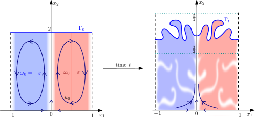
Figure 1: Illustrations of our initial data $u_{0},\Gamma_{0}$ and its evolution after time $t$. Here the red and blue colors represent positive and negative vorticity respectively. As we show in Proposition 3.1, for small initial velocity, the free boundary $\Gamma_{t}$ will be confined within $\frac{3}{2}<x_{2}<\frac{5}{2}$ for all time during the lifespan of a solution. This allows us to estimate $u(t,\cdot)$ near the point $(0,0)$.

To prove Theorem 1.1, a natural starting point is to enforce the same symmetry as [15], with $u_{01}$ odd-in-$x_{1}$ and $u_{02}$ even-in-$x_{1}$ respectively. One can easily check that such symmetry holds for all times (so vorticity remains odd-in-$x_{1}$ for all times). The proof is standard and we include it in Lemma 2.1 for the sake of completeness. In addition, if we set $\omega_{0}=1$ at most of the points in the right half of $\mathcal{D}_{0}$ (except a small measure, since $\omega_{0}$ has to smoothly transition to 0 at $x_{1}=0$ and $x_{1}=1$ due to its oddness), one can check that such property also holds for $\mathcal{D}_{t}$, since in the free boundary setting the vorticity is also preserved along the characteristics.

However, despite these similarities, one faces two major challenges to adapt the proof of [15] to the free boundary setting:

The first issue is the deformation of the domain. Since $\omega_{0}\not\equiv 0$ and $\mathcal{D}_{t}$ is evolving in time, it may deform a lot from the initial domain $\mathcal{D}_{0}$. In general, the free boundary $\Gamma_{t}$ might get very close to the origin, and the nonlinear coupling between $\Gamma_{t}$’s evolution and the velocity field in the bulk of the fluid could destroy the small-scale creation mechanism near the origin in [15]. That being said, we show that this can never happen at any time for small initial data. This is because the free boundary Euler equation with surface tension is known to have a conserved energy $E(t)=K(t)+\sigma L(t)$, where $K(t)$ is the kinetic energy and $L(t)$ is the length of the free boundary. (The energy conservation was shown in [16, 17], and we derive it in Proposition 2.4 for the sake of completeness.) Using this conserved energy, we make the simple but important observation that a flat initial free boundary and a small initial kinetic energy guarantees that the free boundary $\Gamma_{t}$ always stays close to $\Gamma_{0}$, thus can never get close to the origin – see Proposition 3.1 for a precise statement, and see Figure 1 for an illustration.

A more serious problem is the lack of Biot-Savart law in the free boundary setting. Recall that for a fixed domain $D$, given the vorticity $\omega(t,\cdot)$ in $D$ at any moment, the velocity field $u(t,\cdot)$ is uniquely determined by the Biot-Savart law $u=\nabla^{\perp}\varphi$, where the stream function $\varphi$ solves the elliptic equation $\Delta\varphi=\omega$ in $D$ with $\varphi=0$ on $\partial D$. This Biot-Savart law was crucial in [15] to derive pointwise estimates of $u(\cdot,t)$. In contrast, in the free boundary setting, even with $\omega(t,\cdot)$ and $\mathcal{D}_{t}$ given at some time $t$, it is not sufficient to uniquely determine $u(t,\cdot)$ – one also needs to know the normal velocity of the free boundary to determine $u(t,\cdot)$ in the fluid domain. To overcome this challenge, we show that $u(t,\cdot)$ can still be somewhat determined by $\omega(t,\cdot)$ by an approximate Biot-Savart law in Section 3.2, which contains an error term that remains regular and small for all times near the origin. This allows us to obtain a pointwise estimate of $u$ similar to the key lemma in [15, Lemma 3.1], leading to the double-exponential growth of $\|\nabla\omega(t)\|_{L^{\infty}(\mathcal{D}_{t})}$.

Notations

• Let $B_{r}$ be the open disk centered at the origin with radius $r$. In Section 3, we define $\Omega:=\mathbb{T}\times[0,1]$. We also define $\Omega^{+}$ and $\mathcal{D}_{t}^{+}$ as the right half of $\Omega$ and $\mathcal{D}_{t}$, i.e. $\Omega^{+}:=[0,1]\times[0,1]$ and $\mathcal{D}_{t}^{+}:=\mathcal{D}_{t}\cap\{x_{1}\in[0,1]\}$.

• We denote by $C$ universal constants whose values may change from line to line. Any constants with subscripts, such as $C_{i}$, stay fixed once they are chosen.

Acknowledgements

CL is supported by the Hong Kong RGC grant No. CUHK–24304621 and CUHK–14302922. YY is partially supported by the NUS startup grant, MOE Tier 1 grant A-0008491-00-00, and the Asian Young Scientist Fellowship. ZH thanks the hospitality of the Chinese University of Hong Kong. The authors thank Tarek Elgindi for suggesting this problem, and Alexander Kiselev for helpful discussions.

2 Preliminary results

In this section, we collect a few preliminary results on the free boundary Euler equations with surface tension. In Section 2.1, We first demonstrate a symmetry to which 2D free boundary Euler equations conform. Such symmetry corresponds to the odd-in-$x_{1}$ symmetry of vorticity in the fixed boundary case [15], and is crucial to our construction. In Section 2.2, we show the conservation of vorticity and an energy balance involving the bulk kinetic energy as well as the length of the free boundary.

2.1 Symmetry in 2D free boundary Euler equations

To begin with, we discuss some symmetry properties of the 2D free boundary Euler equations. For the 2D Euler equation in fixed domains, the conservation of odd-in-$x_{1}$ symmetry in vorticity is crucial in the proof of small scale formations, as seen in [15, 20, 21]. Below we show that a similar symmetry is also preserved for free boundary Euler equations; the difference is that we state the symmetry assumptions in terms of the velocity rather than the vorticity, since for the free boundary Euler equation one cannot uniquely determine the velocity using the vorticity at a given moment due to the kinematic boundary condition (1.2).

Lemma 2.1.

Let $(u_{0},\mathcal{D}_{0})$ be the initial data of (1.1)–(1.4), where $\mathcal{D}_{0}$ is given by (1.5) and $u_{0}=(u_{01},u_{02})$ satisfies

$$u_{01}(-x_{1},x_{2})=-u_{01}(x_{1},x_{2}),\quad u_{02}(-x_{1},x_{2})=u_{02}(x_{1},x_{2}).$$ (2.1)

Then for all time during the lifespan of a solution, the solution $(u,\mathcal{D}_{t})$ satisfies the same symmetry, i.e.

$$-u_{1}(t,-x_{1},x_{2})=u_{1}(t,x_{1},x_{2}),\quad u_{2}(t,-x_{1},x_{2})=u_{2}(t,x_{1},x_{2}),$$ (2.2)

and the moving fluid domain $\mathcal{D}_{t}$ remains even in $x_{1}$, i.e.,

$$\mathcal{D}_{t}=\widetilde{\mathcal{D}_{t}}:=\{(-x_{1},x_{2}):(x_{1},x_{2})\in\mathcal{D}_{t}\}.$$ (2.3)

Remark 2.2.

As a direct consequence of (2.2), we know the vorticity $\omega(t,x)=\nabla^{\perp}\cdot u(t,x)$ stays odd in $x_{1}$ for all time during the lifespan of a solution.

Proof.

First, setting

$$v(t,x_{1},x_{2})=(v_{1}(t,x_{1},x_{2}),v_{2}(t,x_{1},x_{2})) =(-u_{1}(t,-x_{1},x_{2}),u_{2}(t,-x_{1},x_{2})),$$ (2.4)

$$q(t,x_{1},x_{2}) =p(t,-x_{1},x_{2}),$$ (2.5)

it suffices to show that $(v,q,\widetilde{\mathcal{D}_{t}})$ also verifies the system (1.1)–(1.4) due to uniqueness of solution. Fixing $(x_{1},x_{2})\in\widetilde{\mathcal{D}_{t}}$, a direct computation shows that

$$(\partial_{t}v_{1}+v\cdot\nabla v_{1}+\partial_{1}q)|_{(t,x_{1},x_{2})} =-(\partial_{t}u_{1}+u\cdot\nabla u_{1}+\partial_{1}p)|_{(t,-x_{1},x_{2})},$$

$$(\partial_{t}v_{2}+v\cdot\nabla v_{2}+\partial_{2}q)|_{(t,x_{1},x_{2})} =(\partial_{t}u_{2}+u\cdot\nabla u_{2}+\partial_{2}p)|_{(t,-x_{1},x_{2})},$$

which implies that $\partial_{t}v+v\cdot\nabla v+\nabla q=0$ in $\widetilde{\mathcal{D}_{t}}$. Similarly, we have

$$\nabla\cdot v|_{(t,x_{1},x_{2})}=\nabla\cdot u|_{(t,-x_{1},x_{2})}=0.$$

Second, we need to check the boundary conditions. Since $\partial\widetilde{\mathcal{D}_{t}}=\widetilde{\Gamma}_{t}\cup\widetilde{\Gamma}_{b}$, where

$$\widetilde{\Gamma}_{t}=\{(x_{1},x_{2}):(-x_{1},x_{2})\in\Gamma_{t}\},$$ (2.6)

and $\widetilde{\Gamma}_{b}=\Gamma_{b}$, then it is straightforward to check that $v\cdot n=0$ on $\widetilde{\Gamma}_{b}$.

Furthermore, denoting by $\widetilde{\mathcal{N}}=(\widetilde{\mathcal{N}}_{1},\widetilde{\mathcal{N}}_{2})$ the outward unit normal to $\widetilde{\Gamma}_{t}$, we infer from (2.6) that

$$\widetilde{\mathcal{N}}_{1}(t,x_{1},x_{2})=-\mathcal{N}_{1}(t,-x_{1},x_{2}),\quad\widetilde{\mathcal{N}}_{2}(t,x_{1},x_{2})=\mathcal{N}_{2}(t,-x_{1},x_{2}).$$ (2.7)

This yields $v\cdot\widetilde{\mathcal{N}}|_{(t,x_{1},x_{2})}=u\cdot\mathcal{N}|_{(t,-x_{1},x_{2})}$.

Finally, we define $\widetilde{\mathcal{H}}$ to be the mean curvature of $\widetilde{\Gamma}_{t}$. By definition, $\mathcal{H}=\overline{\nabla}\cdot\mathcal{N},$ where $\overline{\nabla}$ is the spatial derivative tangent to $\Gamma_{t}$, whose components read

$$\overline{\nabla}_{j}=\nabla_{j}-\mathcal{N}_{j}(\mathcal{N}\cdot\nabla),\quad j=1,2.$$

This implies $\widetilde{\mathcal{H}}=\widetilde{\overline{\nabla}}\cdot\widetilde{\mathcal{N}},$ where $\widetilde{\overline{\nabla}}_{j}=\nabla_{j}-\widetilde{\mathcal{N}}_{j}(\widetilde{\mathcal{N}}\cdot\nabla)$. Then, in light of (2.7), a direct computation yields that for any $(x_{1},x_{2})\in\Gamma_{t}$,

$$\widetilde{\mathcal{H}}(t,x_{1},x_{2})=\widetilde{\overline{\nabla}}\cdot\widetilde{\mathcal{N}}|_{(t,x_{1},x_{2})}=\overline{\nabla}\cdot\mathcal{N}|_{(t,-x_{1},x_{2})}=\mathcal{H}(t,-x_{1},x_{2}).$$ (2.8)

Thanks to (2.5), we have

$$q=\sigma\widetilde{\mathcal{H}},\quad\text{ on }\widetilde{\Gamma}_{t}.$$

This concludes the proof. ∎

2.2 Conservation of vorticity and a conserved $L^{2}$-energy

In this subsection, we aim to show two conserved quantities satisfied by the free-boundary Euler equations (1.1) on both vorticity and velocity sides. The first result below shows that, identical to the classical fixed-boundary Euler equations, any $L^{p}$ norm of the vorticity is conserved.

Proposition 2.3.

For any $1\leq p\leq\infty$, we have $\|\omega(t,\cdot)\|_{L^{p}(\mathcal{D}_{t})}=\|\omega_{0}\|_{L^{p}(\mathcal{D}_{0})}$ for all times during the lifespan of the solution.

Proof.

By applying the operator $\nabla^{\perp}\cdot$ to the velocity equation in (1.1) and using the divergence-free property of $u$, $\omega$ satisfies the following transport equation

$$\partial_{t}\omega+u\cdot\nabla\omega=0\quad\text{ in }\mathcal{D}_{t}.$$

This vorticity equation together with the divergence-free property of $u$ yields the result. ∎

The following proposition shows that free boundary Euler equations with surface tension have a conserved $L^{2}$-energy. It plays a pivotal role in quantifying the constraining effect of the surface tension on the behavior of the free boundary, as we will see in Section 3.1.

Proposition 2.4.

Let

$$E(t):=K(t)+\sigma L(t),$$ (2.9)

where

$$K(t):=\frac{1}{2}\int_{\mathcal{D}_{t}}|u(t,x)|^{2}\,dx\quad\text{ and }\quad L(t):=\int_{\Gamma_{t}}dS_{t}$$

are the kinetic energy of the fluid and the length of $\Gamma_{t}$ respectively. Then

$$E(t)=E(0)$$ (2.10)

for all times during the lifespan of the solution.

Proof.

We will verify the identity (2.10) by direct computation. We start from

$$\frac{d}{dt}K(t)=\int_{\mathcal{D}_{t}}(\partial_{t}u+u\cdot\nabla u)\cdot u\,dx=-\int_{\mathcal{D}_{t}}\nabla p\cdot u\,dx,$$

and then apply the divergence theorem and the boundary conditions to obtain

$$-\int_{\mathcal{D}_{t}}\nabla p\cdot u\,dx=-\int_{\Gamma_{t}}p(u\cdot\mathcal{N})\,dS_{t}-\int_{\Gamma_{b}}p\underbrace{(u\cdot n)}_{=0}\,dx_{1}+\int_{\mathcal{D}_{t}}p\underbrace{(\nabla\cdot u)}_{=0}\,dx=-\int_{\Gamma_{t}}p(u\cdot\mathcal{N})\,dS_{t}.$$

Now, invoking the boundary conditions $p=\sigma\mathcal{H}$, and $u\cdot\mathcal{N}=V$ on $\Gamma_{t}$, we have

$$-\int_{\Gamma_{t}}p(u\cdot\mathcal{N})\,dS_{t}=-\int_{\Gamma_{t}}\sigma\mathcal{H}V\,dS_{t}.$$ (2.11)

On the other hand, since $\frac{d}{dt}\int_{\Gamma_{t}}dS_{t}=\int_{\Gamma_{t}}\mathcal{H}(u\cdot\mathcal{N})\,dS_{t}$ (whose proof can be found in [11, Chapter 4]), we have

$$\frac{d}{dt}L(t)=\int_{\Gamma_{t}}\mathcal{H}V\,dS_{t}.$$

Combining this with (2.11), we arrive at

$$\frac{d}{dt}E(t)=\frac{d}{dt}(K(t)+\sigma L(t))=0,$$

finishing the proof. ∎

3 Uniform-in-time estimates for the free boundary problem

In this section, we obtain some uniform-in-time estimates of the free boundary and the velocity field, which are at the heart of the proof of the main theorem of the paper.

3.1 Uniform-in-time control of the free boundary and kinetic energy

The following result shows that if the initial free boundary is flat and the initial kinetic energy is sufficiently small, the free boundary $\Gamma_{t}$ stays constrained in a small neighborhood around the initial profile $\Gamma_{0}$ for all times, and the kinetic energy at time $t$ always stays below the initial kinetic energy.

Proposition 3.1.

Let $\sigma>0$. Consider the solution to the system (1.1)–(1.4) with initial fluid domain $\mathcal{D}_{0}$ given by (1.5), where the initial velocity $u_{0}$ is smooth and has a small kinetic energy $K(0)\leq\frac{\sigma}{20}$. Then we have

$$\Gamma_{t}\subset\mathbb{T}\times\left(\frac{3}{2},\frac{5}{2}\right)\quad\text{for all}\,\,t\in[0,T)$$ (3.1)

and

$$K(t)\leq K(0)\quad\text{for all}\,\,t\in[0,T),$$ (3.2)

where $T>0$ is the lifespan of the solution.

Proof.

In light of (2.10) in Proposition 2.4, we obtain

$$K(t)+\sigma L(t)=K(0)+\sigma L(0)$$ (3.3)

for all times during the lifespan of the solution. Since $K(t)\geq 0$, we have

$$L(t)=L(0)+\frac{K(0)-K(t)}{\sigma}\leq L(0)+\frac{K(0)}{\sigma}\leq 2.05,$$ (3.4)

where the last inequality follows from the assumptions (1.5) (so $L(0)=2$) and $K(0)\leq\frac{\sigma}{20}$.

Also, we deduce from the incompressibility that $\mathcal{D}_{t}$ has the same area as $\mathcal{D}_{0}$, so during the lifespan of the solution, $\Gamma_{t}$ must intersect with $\Gamma_{0}=\mathbb{T}\times\{2\}$ at least once. In addition, $\Gamma_{t}$ is a closed curve in $\mathbb{T}\times\mathbb{R}_{+}$, and its projection onto the $x_{1}$ axis is the whole set $\mathbb{T}$.

For any closed curve satisfying the properties above, if it intersects either $\mathbb{T}\times\{\frac{3}{2}\}$ or $\mathbb{T}\times\{\frac{5}{2}\}$, an elementary computation shows that it must have length at least $2\sqrt{1+(\frac{1}{2})^{2}}=\sqrt{5}\approx 2.236$. Since the length of $\Gamma_{t}$ stays below 2.05 for all times due to (3.4), we conclude that $\Gamma_{t}$ must be contained in $\mathbb{T}\times\left(\frac{3}{2},\frac{5}{2}\right)$ for all times, which proves (3.1).

To show (3.2), note that (3.3) gives $K(t)=K(0)+\sigma(L(0)-L(t))$, where $L(0)=2$. During the lifespan of the solution, the projection of $\Gamma_{t}$ onto the $x_{1}$ axis is the whole set $\mathbb{T}=[-1,1)$, thus $\Gamma_{t}$ has length at least 2. This yields $L(t)\geq 2=L(0)$, thus $K(t)\leq K(0)$. ∎

3.2 Error estimates of an approximate Biot-Savart law

As we have described in the introduction, a major issue in obtaining pointwise velocity estimates in the free boundary setting is the lack of Biot-Savart law, namely, to determine $u(t,\cdot)$, it is not sufficient to know $\omega(t,\cdot)$ and $\mathcal{D}_{t}$. To overcome this challenge, we introduce an “approximate Biot-Savart law” which only uses the information of $\omega(t,\cdot)$ in the set $\Omega:=\mathbb{T}\times[0,1]$, which leads to an approximate velocity field $U(t,\cdot)$ in $\Omega$. We will then use the uniform-in-time estimates in Proposition 3.1 to obtain a precise estimate on the error between the actual velocity $u$ and the approximate velocity field $U$ – it turns out the error is quite regular and small near the origin.

Recall the notations $\Omega:=\mathbb{T}\times[0,1]$, and $B_{r}$ as the open disk centered at the origin with radius $r$. We emphasize that as long as the initial kinetic energy is small, we have $\Omega\subset\mathcal{D}_{t}$ for all times during the lifespan of the solution due to Proposition 3.1.

For any $t\geq 0$ during the lifespan of the solution, we define an approximate velocity field $U(t,\cdot):\Omega\to\mathbb{R}^{2}$ as

$$U(t,\cdot):=\nabla^{\perp}\Phi(t,\cdot)\quad\text{ in }\Omega,$$ (3.5)

where $\Phi(t,\cdot)$ solves the following elliptic equation at the fixed time $t$:

$$\begin{cases}\Delta\Phi(t,\cdot)=\omega(t,\cdot)&\text{ in }\Omega\\ \Phi(t,\cdot)=0&\text{ on }\partial\Omega,\end{cases}$$ (3.6)

where $\omega(t,\cdot)=\nabla^{\perp}\cdot u(t,\cdot)$ is the vorticity of the solution $u(t,\cdot)$.

Note that $U(t,\cdot)$ is uniquely determined by $\omega(t,\cdot)|_{\Omega}$ using the usual Biot-Savart law for 2D Euler equation in the fixed domain $\Omega$, hence the name “approximate Biot-Savart law”. To estimate the error between $U$ and the actual velocity field $u(t,\cdot)|_{\Omega}$ restricted to $\Omega$ (note that $u|_{\Omega}$ is well defined since $\Omega\subset\mathcal{D}_{t}$ for all times by Proposition 3.1), we define the error $e(t,\cdot):\Omega\to\mathbb{R}^{2}$ as

$$e(t,\cdot):=u(t,\cdot)|_{\Omega}-U(t,\cdot).$$ (3.7)

The following proposition plays a key role in our proof of small scale creation. It says that the error $e$ is very regular in $B_{1/2}\cap\Omega$, and $\nabla e$ is pointwise bounded above by $C\sqrt{K(0)}$ for all times. (In fact, the same estimate holds for any higher derivative of $e$, at the expense of having a larger $C$ – but controlling the first derivative of $e$ is sufficient for us.)

Proposition 3.2.

Let $\sigma>0$. Consider the solution to the system (1.1)–(1.4) with initial fluid domain $\mathcal{D}_{0}$ given by (1.5), where the initial velocity $u_{0}$ is smooth and has small kinetic energy $K(0)\leq\frac{\sigma}{20}$. During the lifespan of the solution, let $U(t,\cdot)$ and $e(t,\cdot)$ be defined as in (3.5) and (3.7) respectively.

Then $e(t,\cdot)$ is smooth in $B_{1/2}\cap\Omega$ up to its boundary, and there exists a universal constant $C$ such that

$$\|\nabla e(t,\cdot)\|_{L^{\infty}(B_{1/2}\cap\Omega))}\leq C\sqrt{K(0)}.$$ (3.8)

Proof.

Let us fix any time $t\geq 0$ during the lifespan of a solution. In the following, all functions are at this frozen time $t$, so for notational simplicity, we will omit their $t$ dependence.

First note that $e$ is divergence-free since both $U$ and $u$ are divergence-free in $\Omega$. By Helmholtz decomposition, there exists a stream function $F:\Omega\to\mathbb{R}$ such that

$$e=\nabla^{\perp}F.$$

Moreover, $e$ is also irrotational in $\Omega$: applying $\nabla^{\perp}\cdot$ on both sides of (3.7) (and using the definition of $U$ in (3.5)–(3.6)), we have

$$\nabla^{\perp}\cdot e=\nabla^{\perp}\cdot u-\nabla^{\perp}\cdot\nabla^{\perp}\Phi=\omega-\omega=0\quad\text{ in }\Omega.$$

This leads to

$$\Delta F=\nabla^{\perp}\cdot e=0\quad\text{ in }\Omega.$$

In addition, on $\Gamma_{b}=\mathbb{T}\times\{0\}$, we have $U\cdot n=\nabla^{\perp}\Phi\cdot n=0$ (from the boundary condition $\Phi=0$ on $\Gamma_{b}$) and $u\cdot n=0$ by (1.4). Thus we must also have

$$\nabla^{\perp}F\cdot n=e\cdot n=(u-U)\cdot n=0\quad\text{ on }\Gamma_{b}.$$ (3.9)

This implies $F=\text{const}$ on $\Gamma_{b}$, and by adding a constant to $F$ we have $F(t,\cdot)=0$ on $\Gamma_{b}$ without loss of generality. Combining the above, we have shown that there exists $F(t,\cdot):\Omega\to\mathbb{R}$ such that $e(t,\cdot)=\nabla^{\perp}F(t,\cdot)$, where $F$ satisfies

$$\begin{cases}\Delta F(t,\cdot)=0&\text{ in }\Omega,\\ F(t,\cdot)=0&\text{ on }\Gamma_{b}.\end{cases}$$ (3.10)

To show the regularity estimate (3.8), we first prove a bound for $\|F\|_{H^{1}(\Omega)}$. We observe the following orthogonality property between $\nabla\Phi$ and $\nabla F$ in $\Omega$:

$$\int_{\Omega}\nabla\Phi\cdot\nabla Fdx =-\int_{\Omega}\Phi\underbrace{\Delta F}_{=0}dx+\int_{\partial\Omega}\underbrace{\Phi}_{=0}(n\cdot\nabla F)dS(x)=0,$$

where we used $F$ being harmonic in $\Omega$ and the boundary condition of $\Phi$. Here, $dS(x)$ denotes the induced surface measure on $\partial\Omega$. Taking advantage of the orthogonality and the a priori bound (3.2) for the kinetic energy $K(t)$, we have

$$\int_{\Omega}|\nabla\Phi(t,x)|^{2}+|\nabla F(t,x)|^{2}dx =\|u(t,\cdot)\|_{L^{2}(\Omega)}^{2}\leq 2K(t)\leq 2K(0),$$

from which one obtains $\|\nabla F(t,\cdot)\|_{L^{2}(\Omega)}^{2}\leq 2K(0)$. Now, since $F\equiv 0$ on $\Gamma_{b}$, we infer from Poincaré inequality that

$$\|F(t,\cdot)\|_{H^{1}(\Omega)}^{2}\leq CK(0)$$ (3.11)

for some universal constant $C$. To show the $C^{2}$ bound for $F$, recall that $F$ is harmonic in $\Omega=\mathbb{T}\times[0,1]$ and satisfies the boundary condition $F=0$ on $\Gamma_{b}$. Let us oddly extend $F$ to $\tilde{\Omega}:=\mathbb{T}\times[-1,1]$:

$$\tilde{F}(x):=\begin{cases}F(x_{1},x_{2}),&x_{2}\geq 0,\\ -F(x_{1},-x_{2}),&x_{2}<0\end{cases}\quad\text{ for }x=(x_{1},x_{2})\in\tilde{\Omega}.$$

By the Schwarz Reflection Principle for real harmonic functions, $\tilde{F}:\tilde{\Omega}\to\mathbb{R}$ is harmonic in $\tilde{\Omega}$, thus it is also harmonic in the unit disk $B_{1}\subset\tilde{\Omega}$, and obeys the bound

$$\|\tilde{F}\|_{H^{1}(B_{1})}^{2}\leq\|\tilde{F}\|_{H^{1}(\tilde{\Omega})}^{2}=2\|F\|_{H^{1}(\Omega)}^{2}\leq 2CK(0)$$

by (3.11). Applying the standard Calderón-Zygmund estimate (see [12, Chapter 2]) and Sobolev embedding, we conclude that

$$\|\tilde{F}\|_{C^{2}(B_{1/2})}\lesssim\|\tilde{F}\|_{H^{4}(B_{1/2})}\lesssim\|\tilde{F}\|_{H^{1}(B_{1})}\leq C\sqrt{K(0)},$$

which finishes the proof of (3.8) after recalling $\nabla e=\nabla(\nabla^{\perp}\tilde{F})$ in $B_{1/2}\cap\Omega$. ∎

Note that Proposition 3.2 only uses the smallness of initial kinetic energy, and we have not used the symmetry of initial velocity yet. Under additional symmetry assumptions in Lemma 2.1, we arrive at the following:

Proposition 3.3.

Let the initial data of the system (1.1)–(1.4) satisfy the assumptions of both Proposition 3.2 and Lemma 2.1. Then $e_{1}(t,\cdot)$ is odd in $x_{1}$ and $e_{2}(t,\cdot)$ is even in $x_{1}$ for all times during the lifespan of the solution. Moreover, there exists a universal constant $C$ such that for any $x\in B_{1/2}\cap\Omega$, we have

$$|e_{j}(t,x)|\leq C\sqrt{K(0)}|x_{j}|,\quad j=1,2.$$ (3.12)

Proof.

Using Lemma 2.1, we know $u_{1}(t,x)$ is odd in $x_{1}$ and $u_{2}(t,x)$ is even in $x_{1}$ for all times in $\mathcal{D}_{t}$, thus $\omega(t,x)$ is odd in $x_{1}$ in $\mathcal{D}_{t}$. Since $\Omega\subset\mathcal{D}_{t}$ by Proposition 3.1, this immediately implies that $\Phi(t,x)$ in (3.6) is also odd in $x_{1}$ in $\Omega$, due to uniqueness of solution of (3.6). Using $U(t,x)=\nabla^{\perp}\Phi(t,x)$, $U_{1}(t,x)$ is odd in $x_{1}$ and $U_{2}(t,x)$ is even in $x_{1}$ for all times. Recalling $e=u-U$, we know $e_{1}(t,x)$ and $e_{2}(t,x)$ must satisfy the asserted symmetries in $\Omega$.

To show the estimate (3.12), let us fix any $x\in B_{1/2}\cap\Omega$. First using the fact that $e_{1}(t,0,x_{2})=0$ for $x_{2}\in[0,1]$ due to symmetry, we have

$$|e_{1}(t,x)|=\left|e_{1}(t,x_{1},x_{2})-e_{1}(t,0,x_{2})\right|\leq\|\partial_{1}e_{1}\|_{L^{\infty}(B_{1/2}\cap\Omega)}|x_{1}|\leq C\sqrt{K(0)}|x_{1}|,$$

where we used (3.8) in the last inequality. On the other hand, since $e_{2}(t,x_{1},0)=0$ for $x_{1}\in\mathbb{T}$ by (3.9), a similar argument to the above yields (3.12) with $j=2$. ∎

3.3 Estimating $u$ using integral of $\omega$

With the error estimate above, we are finally ready to state and prove a pointwise velocity estimate that parallels the lemmas in [15, Lemma 3.1] and [21, Lemma 2.1]. In the following, let $\Omega_{+}:=\mathbb{T}_{+}\times[0,1]$.

Proposition 3.4.

Let the initial data of the system (1.1)–(1.4) satisfy the assumptions of both Proposition 3.2 and Lemma 2.1. Then for any $x\in B_{1/2}\cap\Omega_{+}$, the following holds for all time during the lifespan of the solution $[0,T)$:

$$u_{j}(t,x)=(-1)^{j}\frac{4}{\pi}\left(\int_{Q(2x)}\frac{y_{1}y_{2}}{|y|^{4}}\omega(t,y)dy+B_{j}(t,x)\right)x_{j},\quad j=1,2,$$ (3.13)

where $Q(x):=[x_{1},1]\times[x_{2},1]$, and $B_{1}$ and $B_{2}$ satisfies

$$\begin{split}|B_{1}(t,x)|\leq C_{0}\left(\|\omega_{0}\|_{L^{\infty}(\Omega)}\left(1+\log\left(1+\frac{x_{2}}{x_{1}}\right)\right)+\sqrt{K(0)}\right),\\ |B_{2}(t,x)|\leq C_{0}\left(\|\omega_{0}\|_{L^{\infty}(\Omega)}\left(1+\log\left(1+\frac{x_{1}}{x_{2}}\right)\right)+\sqrt{K(0)}\right)\end{split}$$ (3.14)

for some universal constant $C_{0}$.

Proof.

Recall that (3.7) gives

$$u(t,x)=U(t,x)+e(t,x)\quad\text{ for }x\in B_{1/2}\cap\Omega_{+},t\in[0,T).$$

In Proposition 3.3, we have already obtained an estimate for the error term $e(t,x)$, namely

$$|e_{j}(t,x)|\leq C\sqrt{K(0)}x_{j},\quad\text{ for }j=1,2.$$

(Note that $x_{1},x_{2}\geq 0$ since $x\in B_{1/2}\cap\Omega_{+}$). Therefore to show (3.13)–(3.14), it suffices to prove that

$$U_{j}(t,x)=(-1)^{j}\frac{4}{\pi}\left(\int_{Q(2x)}\frac{y_{1}y_{2}}{|y|^{4}}\omega(t,y)dy+\tilde{B}_{j}(t,x)\right)x_{j},\quad j=1,2,$$ (3.15)

where $\tilde{B}_{1},\tilde{B}_{2}$ satisfy (3.14) without the terms $\sqrt{K(0)}$ on the right hand side.

To show this, let $\tilde{\omega}$ be the odd-in-$x_{2}$ extension of $\omega$ from $\Omega=\mathbb{T}\times[0,1]$ to $\mathbb{T}^{2}$, i.e.

$$\tilde{\omega}(t,x_{1},x_{2}):=\begin{cases}\omega(t,x_{1},x_{2}-2n_{2}),&x_{2}\in(2n_{2},1+2n_{2})\\ -\omega(t,x_{1},-(x_{2}-2n_{2})),&x_{2}\in(-1+2n_{2},2n_{2})\end{cases}\quad\text{ for all }n_{2}\in\mathbb{Z}.$$

Since $\tilde{\omega}$ is odd in $x_{1}$ (by Lemma 2.1) and odd in $x_{2}$ (by definition of $\tilde{\omega}$), there exists a unique odd-odd solution $\Psi(t,\cdot)$ to the equation

$$\Delta\Psi(t,\cdot)=\tilde{\omega}(t,\cdot)\quad\text{ in }\mathbb{T}^{2},$$ (3.16)

and $\Psi\in C^{1,\alpha}(\mathbb{T}^{2})$ for any $\alpha\in(0,1)$. Note that $\Psi=0$ on both $\mathbb{T}\times\{x_{2}=0\}$ and $\mathbb{T}\times\{x_{2}=1\}$ since $\tilde{\omega}$ is odd about both lines. This implies $\Psi=0=\Phi$ on $\partial\Omega$. Combining this with $\Delta\Psi=\omega=\Delta\Phi$ in $\Omega$ leads to $\Psi=\Phi$ in $\Omega$, therefore $U=\nabla^{\perp}\Phi=\nabla^{\perp}\Psi$.

Note that for any $x\in\Omega$, we can express $\Psi(t,x)$ using the Newtonian potential as

$$\Psi(t,x)=\frac{1}{2\pi}\sum_{n\in\mathbb{Z}^{2}}\int_{[-1,1]^{2}}\ln|x-y-2n|\,\tilde{\omega}(t,y)dy$$

(note that the sum converges since $\tilde{\omega}$ has mean zero in $[-1,1]^{2}$), which leads to the following representation of $U$:

$$U(t,x) =\nabla^{\perp}\Psi(t,x)=\frac{1}{2\pi}\sum_{n\in\mathbb{Z}^{2}}\int_{[-1,1]^{2}}\frac{(x_{2}-y_{2}-2n_{2},-x_{1}+y_{1}+2n_{1})}{|x-y-2n|^{2}}\tilde{\omega}(t,y)dy.$$

This is exactly the Biot-Savart law for 2D Euler equation in $\mathbb{T}^{2}$, therefore we can directly use the estimate in [21, Lemma 2.1] to obtain (3.15), where $\tilde{B}_{1}$ and $\tilde{B}_{2}$ satisfy

$$|\tilde{B}_{1}(t,x)|\leq C\|\omega_{0}\|_{L^{\infty}(\Omega)}\left(1+\min\left\{\log\left(1+\frac{x_{2}}{x_{1}}\right),x_{2}\frac{\|\nabla\omega(t,\cdot)\|_{L^{\infty}([0,2x_{2}]^{2})}}{\|\omega_{0}\|_{L^{\infty}(\Omega)}}\right\}\right),$$ (3.17)

$$|\tilde{B}_{2}(t,x)|\leq C\|\omega_{0}\|_{L^{\infty}(\Omega)}\left(1+\min\left\{\log\left(1+\frac{x_{1}}{x_{2}}\right),x_{1}\frac{\|\nabla\omega(t,\cdot)\|_{L^{\infty}([0,2x_{1}]^{2})}}{\|\omega_{0}\|_{L^{\infty}(\Omega)}}\right\}\right)$$ (3.18)

for some universal constant $C$. This finishes the proof: note that we can simply drop the second argument in the minimum to arrive at $|\tilde{B}_{j}(t,x)|\leq C\|\omega_{0}\|_{L^{\infty}}(1+\log((1+\frac{x_{3-j}}{x_{j}}))$ for $j=1,2$. ∎

4 Proof of the main theorem

Once Proposition 3.4 is established, the rest of the proof is largely parallel to the proof of [15, Theorem 1.1]. However, the situation is slightly more delicate here due to the presence of $\varepsilon$: recall that our initial velocity $u_{0}=\varepsilon v_{0}$ depends on $\varepsilon$ since we want to show double-exponential growth can happen for arbitrarily small $\varepsilon\ll 1$. In our proof, we need to construct $v_{0}$ that is independent of $\varepsilon$, and we need to carefully justify that the double-exponential growth phenomenon happens for any small $\varepsilon$, and quantify the growth rate (which depends on $\varepsilon$).

Proof of Theorem 1.1.

Recall that the initial velocity is set as $u_{0}=\varepsilon v_{0}$ with $\varepsilon$ sufficiently small, where $v_{0}\in C^{\infty}(\mathcal{D}_{0})$ is a fixed velocity field independent of $\varepsilon$. We define $v_{0}$ as $v_{0}:=\nabla^{\perp}\phi$, where $\phi$ solves

$$\begin{cases}\Delta\phi=f&\text{ in }\mathcal{D}_{0},\\ \phi=0&\text{ on }\partial\mathcal{D}_{0}.\end{cases}$$

Here $f\in C^{\infty}(\mathcal{D}_{0})$ is odd in $x_{1}$, and satisfies $0\leq f\leq 1$ in $\mathcal{D}_{0}^{+}$ and $f(x_{1},x_{2})=1$ for $x_{1}\in[\kappa^{10},1-\delta]$, where $\kappa$ and $\delta$ are small universal constants satisfying $0<\kappa<\delta<\frac{1}{2}$, and they will be fixed momentarily. Since $\|f\|_{L^{\infty}(\mathcal{D}_{0})}=1$ regardless of $\kappa$ and $\delta$, a standard elliptic estimate gives $\|v_{0}\|_{L^{2}(\mathcal{D}_{0})}\leq\|\phi\|_{H^{1}(\mathcal{D}_{0})}\leq C$ for some universal constant $C$, which implies

$$K(0)=\frac{1}{2}\|u_{0}\|_{L^{2}(\mathcal{D}_{0})}^{2}=\frac{\varepsilon^{2}}{2}\|v_{0}\|_{L^{2}(\mathcal{D}_{0})}^{2}\leq C_{1}\varepsilon^{2}$$ (4.1)

for some universal $C_{1}$. Therefore, setting $\varepsilon_{0}:=(20C_{1})^{-1/2}$, we have $K(0)\leq\frac{1}{20}$ for all $\varepsilon\in(0,\varepsilon_{0})$. Thus for all $\varepsilon\in(0,\varepsilon_{0})$, the initial velocity $u_{0}$ constructed as above satisfies the small kinetic energy assumption in Proposition 3.1 and 3.2 (recall that we set $\sigma=1$ in the assumption of Theorem 1.1). As a result, Proposition 3.1 implies $\Omega\subset\mathcal{D}_{t}$ for all $t\in[0,T)$. Due to the odd-in-$x_{1}$ symmetry of $f$, $u_{0}$ also satisfies the symmetry assumption in Lemma 2.1.

Since the initial vorticity is $\omega_{0}=\varepsilon f$ in $\mathcal{D}_{0}$, the set $\{x\in\mathcal{D}_{0}^{+}:\omega_{0}(x)\neq\varepsilon\}$ has area less than $2\delta$. Using the incompressibility of the flow and the conservation of $\omega$ along the flow map, for any time $t\in[0,T)$, the set $\{x\in\mathcal{D}_{t}^{+}:\omega(t,x)\neq\varepsilon\}$ has area less than $2\delta$. This fact allows us to obtain a lower bound of the integral in (3.13) using a similar argument as [15, Eq.(3.15)]: for any $t\in[0,T)$ and $x\in B_{\delta}\cap\Omega_{+}$,

$$\int_{Q(2x)}\frac{y_{1}y_{2}}{|y|^{4}}\omega(y)dy\geq\frac{1}{4}\int_{2\delta}^{1}\int_{\pi/6}^{\pi/3}\frac{\omega(r,\theta)}{r}d\theta dr\geq\frac{\varepsilon}{4}\int_{4\sqrt{\delta}}^{1}\int_{\pi/6}^{\pi/3}\frac{1}{r}d\theta dr=\frac{\varepsilon\pi}{48}(\log\delta^{-1}-2\log 4),$$ (4.2)

where the first inequality uses the definition of $Q(2x)$ and the fact that $\omega\geq 0$ in $Q(2x)$, and the second inequality uses $|\{x\in\mathcal{D}_{t}^{+}:\omega(t,x)\neq\varepsilon\}|<2\delta$: in the polar integral of $\omega/r$ if we remove a set with area $2\delta$ closest to the origin from the integral domain $\{r\in(2\delta,1),\theta\in(\frac{\pi}{6},\frac{\pi}{3})\}$ to reflect the worst-case scenario that minimizes the integral, the remaining set would have inner radius less than $4\sqrt{\delta}$. Also, applying (4.1) together with the fact that $\|\omega(t,\cdot)\|_{L^{\infty}}=\|\omega_{0}\|_{L^{\infty}}=\varepsilon$, we can control the terms $B_{1}$ and $B_{2}$ in (3.14) as

$$|B_{1}(t,x)|\leq C_{0}\varepsilon(2+\sqrt{C_{1}})=:C_{2}\varepsilon \quad\text{ in }B_{\delta}\cap\Omega_{+}\cap\{0\leq x_{2}\leq x_{1}\}$$ (4.3)

$$|B_{2}(t,x)|\leq C_{0}\varepsilon(2+\sqrt{C_{1}})=:C_{2}\varepsilon \quad\text{ on }B_{\delta}\cap\Omega_{+}\cap\{x_{2}=x_{1}\}.$$ (4.4)

From now on, we fix $\delta\in(0,\frac{1}{2})$ as a small universal constant such that

$$\frac{4}{\pi}\left(\frac{\pi}{48}\left(\log\delta^{-1}-2\log 4\right)-C_{2}\right)>1.$$ (4.5)

With such definition, combining the estimates (3.13) and (4.2)–(4.4), we have

$$-u_{1}(t,x) \geq\varepsilon x_{1}\quad\text{ in }B_{\delta}\cap\Omega_{+}\cap\{0\leq x_{2}\leq x_{1}\}$$ (4.6)

$$u_{2}(t,x) \geq\varepsilon x_{2}\quad\text{ on }B_{\delta}\cap\Omega_{+}\cap\{x_{2}=x_{1}\}.$$ (4.7)

In particular, (4.6) implies the flow map starting from $(\delta,0)$ (denote it by $\eta(t,\delta,0)$) satisfies

$$\eta_{1}(t,\delta,0)\leq\delta e^{-\varepsilon t},$$ (4.8)

where we used the fact that $\eta(t,\delta,0)$ stays on the bottom boundary $\Gamma_{b}$ for all times. Since $\omega(t,\eta(t,\delta,0))=\omega_{0}(\delta,0)=\varepsilon$, we know $\|\nabla\omega(t)\|_{L^{\infty}}$ at least increases exponentially for all times during the lifespan of a solution:

$$\|\nabla\omega(t,\cdot)\|_{L^{\infty}(\mathcal{D}_{t})}\geq\frac{|\omega(t,\eta(t,\delta,0))|}{|\eta_{1}(t,\delta,0)|}\geq\frac{\varepsilon}{\delta e^{-\varepsilon t}}=\varepsilon\delta^{-1}e^{\varepsilon t}.$$

To upgrade the exponential growth to double-exponential growth, we follow the same argument as [15], except that we have to keep track of the dependence on $\varepsilon$ in the growth rate. For any $t>0$ and $x_{1}\in(0,1)$, we define the following two velocities (which is well-defined since $\Omega\subset\mathcal{D}_{t}$ for all $t\in[0,T)$):

$$\underaccent{\bar}{u}_{1}(t,x_{1}):=\min_{(x_{1},x_{2})\in\Omega_{+},x_{2}<x_{1}}u_{1}(t,x_{1},x_{2}),\quad\bar{u}_{1}(t,x_{1}):=\max_{(x_{1},x_{2})\in\Omega_{+},x_{2}<x_{1}}u_{1}(t,x_{1},x_{2}),$$ (4.9)

where $\underaccent{\bar}{u}_{1}$ and $\bar{u}_{1}$ are locally Lipschitz in $x_{1}$ during the lifespan of the solution. We then define the functions $a(t)$, $b(t)$ via the ODEs

$$a^{\prime}(t) =\bar{u}_{1}(t,a(t)),\quad a(0)=\kappa^{10},$$ (4.10)

$$b^{\prime}(t) =\underaccent{\bar}{u}_{1}(t,b(t)),\quad b(0)=\kappa.$$ (4.11)

We also define the following trapezoidal region: for $0<x_{1}^{\prime}<x_{1}^{\prime\prime}<1$, let

$$\mathcal{O}(x_{1}^{\prime},x_{1}^{\prime\prime}):=\{(x_{1},x_{2})\in\Omega^{+}\;:\;x_{1}^{\prime}<x_{1}<x_{1}^{\prime\prime},~{}0\leq x_{2}\leq x_{1}\}.$$

And we set

$$\mathcal{O}_{t}:=\mathcal{O}(a(t),b(t)).$$

The choice of our initial data gives $\omega_{0}\equiv\varepsilon$ in $\mathcal{O}_{0}$. We can argue in the same way as [15, page 1215] that $\omega(t,\cdot)\equiv\varepsilon$ in $\mathcal{O}_{t}$: due to the definition of (4.9)–(4.11), we only need to show $u\cdot(-1,1)>0$ along the diagonal of $\mathcal{O}_{t}$. This is true since $u_{1}<0$ and $u_{2}>0$ on the diagonal $B_{\delta}\cap\Omega^{+}\cap\{x_{1}=x_{2}\}$, which follows from (4.6)–(4.7).

Using (4.6), we have

$$b(t)\leq\kappa e^{-\varepsilon t}.$$ (4.12)

To obtain a faster decay for $a(t)$, note that $\log a(t)$ satisfies the differential inequality

$$\begin{split}\frac{d}{dt}\log a(t)&=\frac{\bar{u}_{1}(t,a(t))}{a(t)}\leq-\frac{4}{\pi}\left(\int_{Q(2a(t),2a(t))}\frac{y_{1}y_{2}}{|y|^{4}}\omega(t,y)dy-C_{2}\varepsilon\right)\\ &\leq-\frac{4}{\pi}\left(\int_{Q(2a(t),0)}\frac{y_{1}y_{2}}{|y|^{4}}\omega(t,y)dy-(C_{2}+C_{3})\varepsilon\right).\end{split}$$

where the first inequality follows from (3.13) and (4.3), and the second inequality follows from $\omega\leq\epsilon$ and the fact that for any $a<\frac{1}{2}$, the integral in the rectangle $\int_{[2a,1]\times[0,2a]}\frac{y_{1}y_{2}}{|y|^{4}}dy$ is bounded by a universal constant $C_{3}$. On the other hand, using (3.13) and (4.3), $\log b(t)$ satisfies the differential inequality in the opposite direction:

$$\frac{d}{dt}\log b(t)=\frac{\underaccent{\bar}{u}_{1}(t,b(t))}{b(t)}\geq-\frac{4}{\pi}\left(\int_{Q(2b(t),0)}\frac{y_{1}y_{2}}{|y|^{4}}\omega(t,y)dy+C_{2}\varepsilon\right).$$

Subtracting them yields the following (where we use that $\mathcal{O}(2a(t),b(t))\subset Q(2a(t),0))\setminus Q(2b(t),0))$):

$$\frac{d}{dt}\log\frac{b(t)}{a(t)}\geq\frac{4}{\pi}\left(\int_{\mathcal{O}(2a(t),b(t))}\frac{y_{1}y_{2}}{|y|^{4}}\omega(t,y)dy-(2C_{2}+C_{3})\varepsilon\right).$$ (4.13)

Using $\omega(t,\cdot)\equiv\varepsilon$ in $\mathcal{O}(2a(t),b(t))\subset\mathcal{O}_{t}$, we can bound the integral in (4.13) from below as

$$\int_{\mathcal{O}(2a(t),b(t))}\frac{y_{1}y_{2}}{|y|^{4}}\omega(t,y)dy\geq\varepsilon\int_{0}^{\pi/4}\int_{2a(t)/\cos\theta}^{b(t)/\cos\theta}\frac{\sin 2\theta}{2r}drd\theta=\frac{\varepsilon}{4}\left(\log\frac{b(t)}{a(t)}-\log 2\right),$$

and plugging it into (4.13) gives

$$\frac{d}{dt}\log\frac{b(t)}{a(t)}\geq\varepsilon\left(\frac{1}{\pi}\log\frac{b(t)}{a(t)}-C_{4}\right),$$

where $C_{4}:=\frac{4}{\pi}(\frac{\log 2}{4}+2C_{2}+C_{3})$ is a universal constant. Solving this differential inequality gives

$$\log\frac{b(t)}{a(t)}\geq\exp\left(\frac{\varepsilon t}{\pi}\right)\left(\log\frac{b(0)}{a(0)}-\pi C_{4}\right).$$ (4.14)

Since $\log\frac{b(0)}{a(0)}=9\log\kappa^{-1}$, we can choose $\kappa\in(0,\delta)$ to be a sufficiently small universal constant such that $\log\frac{b(0)}{a(0)}-\pi C_{4}>2$. Note that such choice of $\kappa$ guarantees that $2a(t)<b(t)$ for any $t\in[0,T)$. Hence, (4.14) implies the following (where we use $b(t)\leq 1$ for all $t$ due to (4.12)):

$$a(t)^{-1}\geq\exp\left(2\exp\left(\frac{\varepsilon t}{\pi}\right)\right)b(t)^{-1}\geq\exp\left(2\exp\left(\frac{\varepsilon t}{\pi}\right)\right).$$

Finally, using $\omega\equiv\varepsilon$ in $\mathcal{O}_{t}$, we have $\omega(t,a(t),0)=\varepsilon$, thus combining it with $\omega(t,0,0)=0$ gives

$$\|\nabla\omega(t,\cdot)\|_{L^{\infty}(\mathcal{D}_{t})}\geq\frac{\varepsilon}{a(t)}\geq\varepsilon\exp\left(2\exp\left(\frac{\varepsilon t}{\pi}\right)\right)$$

for all times during the lifespan of the solution. ∎

5 Discussions

At the end, we discuss some generalizations of Theorem 1.1, and state some open questions.

1. Adding gravity to the system. When a gravity force $-ge_{2}$ is added to the first equation of (1.1), where $g>0$ and $e_{2}=(0,1)^{T}$, the system becomes the 2D gravity-capillary water wave system. Our proof can be easily adapted to this case for $g>0$ and $\sigma>0$. This is because the gravity-capillary water wave system enjoys a similar conserved energy $E(t)=K(t)+gP(t)+\sigma L(t),$ where $P(t)=\int_{\mathcal{D}_{t}}x_{2}dx$ is the potential energy. It is simple to check that $P(t)\geq P(0)$ for all $t$, since among all sets with the same area as $\mathcal{D}_{0}$, the set $\mathcal{D}_{0}$ itself given by (1.5) has the lowest potential energy. As a result, the uniform-in-time estimates in Proposition 3.1 still hold. One can also check that adding gravity still preserves the symmetry in Lemma 2.1. The rest of the proof can be carried out without any changes, and we leave the details to interested readers.

2. Removing surface tension. It seems challenging to obtain growth results without surface tension. When $\sigma=0$, the uniform-in-time estimate (3.1) on the free boundary fails, thus the free boundary could potentially get very close to the origin. This difficulty persists even with an additional gravity term – for gravity water wave without surface tension, if the initial kinetic energy is small, using the conserved energy $K(t)+gP(t)=K(0)+gP(0)$ one can prove that the free boundary stays close to $\Gamma_{0}$ in the $L^{2}$ distance for all times, however, their $L^{\infty}$ difference can still be large.

3. Different domains. A natural question is whether the growth result holds for different domains. When the bottom boundary is a graph $\{x_{2}=g(x_{1}):x_{1}\in\mathbb{T}\}$ where $g$ is smooth and even-in-$x_{1}$, we expect the proof would still hold after some modifications, where the estimate of Biot-Savart law in domains with a symmetry axis by Xu [20] could be useful. However, adapting the proof to the infinite-depth case (where there is no bottom boundary) requires substantial new ideas. We also point out that our proof crucially relies on the periodic-in-$x_{1}$ setting, and it is an interesting open question to prove similar results for the $x_{1}\in\mathbb{R}$ case for finite-energy smooth initial data.

References

• [1] Alazard, T., Burq, N., and Zuily, C. On the water-wave equations with surface tension. Duke Mathematical Journal 158, 3 (2011), 413–499.
• [2] Castro, A., CΓ³rboda, D., Fefferman, C., Gancedo, F., and GΓ³mez-Serrano, J. Finite time singularities for the free boundary incompressible Euler equations. Annals of Mathematics (2013), 1061–1134.
• [3] Castro, A., CΓ³rdoba, D., Fefferman, C., Gancedo, F., and GΓ³mez-Serrano, J. Finite time singularities for water waves with surface tension. Journal of Mathematical Physics 53, 11 (2012).
• [4] Castro, A., CΓ³rdoba, D., Fefferman, C.Β L., Gancedo, F., and GΓ³mez-Serrano, J. Splash singularity for water waves. Proceedings of the National Academy of Sciences 109, 3 (2012), 733–738.
• [5] Castro, A., and Lannes, D. Well-posedness and shallow-water stability for a new Hamiltonian formulation of the water waves equations with vorticity. Indiana University Mathematics Journal (2015), 1169–1270.
• [6] Coutand, D., and Shkoller, S. Well-posedness of the free-surface incompressible Euler equations with or without surface tension. Journal of the American Mathematical Society 20, 3 (2007), 829–930.
• [7] Coutand, D., and Shkoller, S. On the finite-time splash and splat singularities for the 3-D free-surface Euler equations. Communications in Mathematical Physics 325 (2014), 143–183.
• [8] Deng, Y., Ionescu, A.Β D., Pausader, B., and Pusateri, F. Global solutions of the gravity-capillary water-wave system in three dimensions. Acta Math. 219 (2017), 213–402.
• [9] Disconzi, M.Β M., and Kukavica, I. A priori estimates for the free-boundary Euler equations with surface tension in three dimensions. Nonlinearity 32, 9 (2019), 3369.
• [10] Disconzi, M.Β M., Kukavica, I., and Tuffaha, A. A Lagrangian interior regularity result for the incompressible free boundary Euler equation with surface tension. SIAM Journal on Mathematical Analysis 51, 5 (2019), 3982–4022.
• [11] Ecker, K. Regularity theory for mean curvature flow, vol.Β 57. Springer Science & Business Media, 2012.
• [12] FernΓ‘ndez-Real, X., and Ros-Oton, X. Regularity Theory for Elliptic PDE. EMS Press, dec 2022.
• [13] Ifrim, M., and Tataru, D. The lifespan of small data solutions in two dimensional capillary water waves. Archive for Rational Mechanics and Analysis 225 (2017), 1279–1346.
• [14] Ionescu, A., and Pusateri, F. Global regularity for 2D water waves with surface tension, vol.Β 256. American Mathematical Society, 2018.
• [15] Kiselev, A., and Ε verΓ‘k, V. Small scale creation for solutions of the incompressible two-dimensional Euler equation. Annals of mathematics 180, 3 (2014), 1205–1220.
• [16] Schweizer, B. On the three-dimensional Euler equations with a free boundary subject to surface tension. Ann. Inst. H. PoincarΓ© C Anal. Non LinΓ©aire 22, 6 (2005), 753–781.
• [17] Shatah, J., and Zeng, C. Geometry and a priori estimates for free boundary problems of the Euler’s equation. Communications on Pure and Applied Mathematics 61, 5 (2008), 698–744.
• [18] Shatah, J., and Zeng, C. A priori estimates for fluid interface problems. Communications on Pure and Applied Mathematics 61, 6 (2008), 848–876.
• [19] Shatah, J., and Zeng, C. Local well-posedness for fluid interface problems. Archive for rational mechanics and analysis 199, 2 (2011), 653–705.
• [20] Xu, X. Fast growth of the vorticity gradient in symmetric smooth domains for 2D incompressible ideal flow. Journal of Mathematical Analysis and Applications 439, 2 (2016), 594–607.
• [21] ZlatoΕ‘, A. Exponential growth of the vorticity gradient for the Euler equation on the torus. Advances in Mathematics 268 (2015), 396–403.