Padding Aware Neurons

Abstract

Convolutional layers are a fundamental component of most image-related models. These layers often implement by default a static padding policy (e.g., zero padding), to control the scale of the internal representations, and to allow kernel activations centered on the border regions. In this work we identify Padding Aware Neurons (PANs), a type of filter that is found in most (if not all) convolutional models trained with static padding. PANs focus on the characterization and recognition of input border location, introducing a spatial inductive bias into the model (e.g., how close to the input’s border a pattern typically is). We propose a method to identify PANs through their activations, and explore their presence in several popular pre-trained models, finding PANs on all models explored, from dozens to hundreds. We discuss and illustrate different types of PANs, their kernels and behaviour. To understand their relevance, we test their impact on model performance, and find padding and PANs to induce strong and characteristic biases in the data. Finally, we discuss whether or not PANs are desirable, as well as the potential side effects of their presence in the context of model performance, generalisation, efficiency and safety.

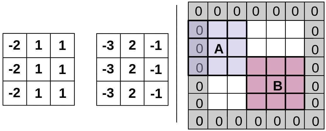
Figure 1: On the left, example of two left Padding Aware Neuron (PAN) filters. Activations on left-border locations (A) give larger outputs than in the centre (location B). On the right border, outputs are also slightly distinct. An actual neuron behaving analogously to the centre kernel can be appreciated in Figure 6.

1 Introduction

Convolution has passed the test of time. Older than its competitors [7], convolutional neurons have been successfully integrated with memory-based models (e.g., LSTM [13], GRU [27]), attention-based architectures [25] and generative tasks [19]. However, convolution has an undesired side-effect: the implicit reduction of internal representations [1] caused by the impossibility of applying the convolved filter on border locations. To avoid this reduction, the most frequently used technique is padding, adding synthetic data around the border of the input, so that kernels can activate there, and produce an output for every input.

The most popular padding type is, by far and wide, zero-padding (adding zeros to the input border). That is, a static padding, the same for every sample and location. Previous works noticed this constant signal adds a bias that reduces generalisation [2, 17, 1, 14], and several dynamic padding methods have been proposed to prevent it [12, 23, 17, 27], with very limited adoption . The reason for this popularity is simple: models obtain better top-of-the-line metrics with static padding, when trained and tested on data from the same source. So far, the padding bias has been excused.

In this work we dig deeper into how padding influences models. To do so, we provide evidence on how much model complexity is dedicated to the data edge bias (between 1% and 3%), and the magnitude of this shortcut in the model’s outcome. This is characterized by the presence of padding aware neurons (PANs), a symptom of padding bias. Our work shows how PANs are likely present in the vast majority of models trained with static padding, and proposes a diagnosis methodology which allows to locate them through their activation patterns.

2 Setting

This work has been implemented using PyTorch 1.12.0 [18], torchvision 0.13.0 [16], numpy 1.23.1 [9] and scipy 1.8.1 [22], the latter for Kolgomorov-Smirnov statistics. All models are provided pre-trained by PyTorch. These are:

• ResNet-50 [10], trained on ILSVRC2012[20], named ResNet101_Weights.IMAGENET1K_V2 in torchvision.

• MobileNetV3 [11], trained on ILSVRC2012, named MobileNet_V3_Large_Weights.IMAGENET1K_V2 in torchvision.

• GoogLeNet [21], trained on ILSVRC2012, named GoogLeNet_Weights.IMAGENET1K_V1 in torchvision.

For each of these models, we analyse all convolutional layers with kernels bigger than 1x1. Notice these pre-trained models are frequently used as source for fine-tuning other models.

We use a random batch from Caltech101 [6] in §3, for generating activations. In §4 we use the validation split of ILSVRC2012 for assessing bias. The code necessary to reproduce the experiments of this work can be found in https://gitlab.com/paper14/padding-aware-neurons.

3 Definition & Analysis

Padding aware neurons, or PANs for short, are convolutional filters that learn to recognise the padding added to the input by some layers (e.g., a convolutional layer). PANs pass information on border location through the network, introducing a spatial bias into the model which may or may not be desirable, depending on the domain of application [2]. Padding is often implemented as a vertical or horizontal edge (e.g., zero padding), which makes PANs a type of edge detector. Edge detectors are fundamental vision kernels. The most popular ones include Prewitt, Sobel and the Laplacian of Gaussian (shown in Figure 2). These kernels look for value contrasts anywhere in the input[15, 24], but are maximised when the value contrast is centred on the kernel (e.g., centre square of a 3x3). This is visible in the symmetry exhibited by the filters of Figure 2. On the edges defined by padding, which are never centred on the kernel, edge detectors still activate moderately. In contrast to a regular edge detector, a PAN would maximize its output when the edge is located at the border of the filter, in order to discriminate the padding edges from other edges in the input. An example of one such kernels are shown in Figure 1.

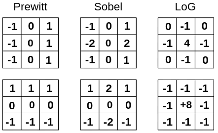
Figure 2: Traditional edge detector filters. Prewitt (1st col.), Sobel (2nd col.) and Laplacian of Gaussian (3rd col.).

We hypothesise the existence of two types of PANs: nascent and downstream. Nascent PANs react when directly exposed to a padding area of the inputs of their layer, while downstream PANs react to the presence of padding as conveyed by PANs in previous layers (i.e., they do not directly perceive padded values). In this work we focus on nascent PANs, which may have a configuration analogous to the kernel shown in Figure 1. Beyond these toy examples, we consider any neuron that activates distinctively – be it strongly or weakly – on padded areas as a PAN. Notice a PAN can react to one or more borders of the input. These include top row (T), bottom row (B), left-most column (L) and right-most column (R), but also any combination of these (i.e., T, B, L, R, TB, TL, TR, BL, BR, LR, TBL, TBR, BLR and TBLR) in their non-overlapping definition (e.g., T $\cap$ BT = $\emptyset$).

3.1 Finding Edge Detectors

Considering the complexities of characterising PANs through their high dimensional kernels [8, 3], we decide to use their activations instead. Next, we propose a method to identify nascent PANs by looking at the activations they produce on a padded input sampling. To be precise, we consider four padding regions of the input ($top$ and $bottom$ rows, $left$ and $right$ columns, all with corner overlap) of size one pixel on the short axis, and the remaining of the input ($centre$, with no overlap). We record the activations a given neuron produces on those five regions while processing a batch of in-distribution data.

From these activations, we obtain five empirical probability density functions (PDF) per neuron ($A_{top}$, $A_{bottom}$, $A_{left}$, $A_{right}$, $A_{centre}$). By comparing every border PDF against $A_{centre}$ we obtain four Kolgomorov-Smirnov test (KS), which measure how distinct padding activations are for a given neuron. At this point its important to notice the sample size difference between border and center activations. $A_{top}$, $A_{bottom}$, $A_{left}$, $A_{right}$ all include the same number of values, $N$. $A_{centre}$ on the other hand includes $(N-2)^{2}$ activations, which grow quadratically w.r.t. $N$ assuming a stride of one.

There is another difference between border and central activations. While border regions are entirely composed by edge data (the one defined by padding), central areas are partly so. While $A_{top}$, $A_{bottom}$, $A_{left}$ and $A_{right}$ contain only edge activations, $A_{centre}$ contains a majority of non-edge activations and a few data-driven edge activations. This skews the centre PDF w.r.t. the border ones, and turns the KS statistic into a measure of how distinctively are edge activations. A sort of padding-like edge detector. Notice this method can not find edge detectors which are not straight vertical or horizontal. Figure 3 shows an example of border and centre PDFs for two neurons, together with the corresponding $KS$ values while using the two-sided KS, where the null hypothesis is that the two distributions are identical.

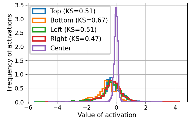
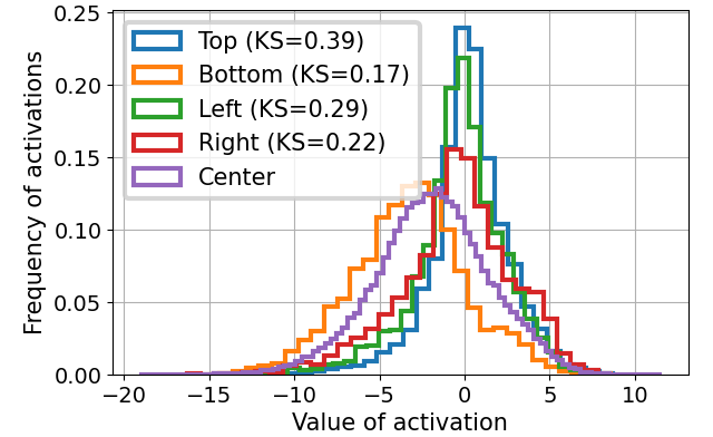
Figure 3: $A_{top}$, $A_{bottom}$, $A_{left}$, $A_{right}$ and $A_{centre}$ PDFs for two convolutional neurons of the ResNet50. Legend shows KS value of centre against every border region. Top plot: Neuron 51 from layer conv_1, an edge detector. Bottom plot: Neuron 101 from layer conv2_2, a regular neuron.

Computing the KS values for all neurons in a model shows the overall activation divergence between centre and border locations. The KS distributions shown in Figure 4 indicate most neurons have low KS values regardless of layer depth, with a mean KS between 0.1 and 0.3 on all cases. In other words, most convolutional neurons have no discriminative power between activations in a padded border and the centre. Notice each neuron contributes with 4 values to each plot of Figure 4 ($KS(A_{top},A_{centre})$, $KS(A_{bottom},A_{centre})$, $KS(A_{left},A_{centre})$ and $KS(A_{right},A_{centre})$), which causes more KS values to be close to zero (e.g., a vertical edge detector will most often generate low KS values for the top and bottom PDFs). Overall, results that indicate potential edge detector and PAN neurons (those with high KS values) are a minority found in most layers, regardless of depth.

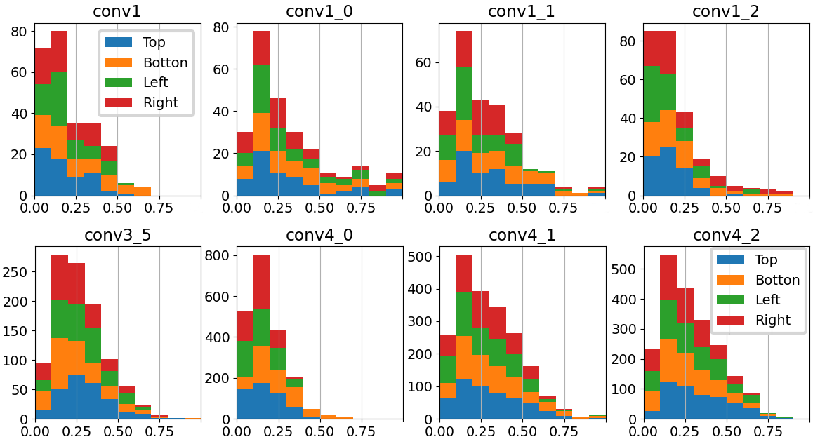
Figure 4: Stacked distribution of KS distances for the first and last four convolutional 3x3 layers of the ResNet50. Notice each neuron contributes with four values to each plot, $KS(A_{top},A_{centre})$, $KS(A_{bottom},A_{centre})$, $KS(A_{left},A_{centre})$ and $KS(A_{right},A_{centre})$.

3.2 Finding PANs

A KS test between the complete $A_{centre}$ and a border PDF cannot properly discriminate between PANs and the rest of edge detectors, as the presence of non-edge activations in $A_{centre}$ dominates its PDF. To discriminate PANs from regular edge detectors using the KS test, we need a distribution of $A_{centre}$ PDF which is comparable to border PDFs, that is, one which contains only edge activations. To that end, we define a simple hypothesis: the centre region of an input (of size $(N-1)^{2}$) will include at least as many edges as a padded border (of size $N$). Notice this hypothesis, as well as the PDF reliability, grows weaker with the reduced input sizes typical of deeper layers.

Leveraging this hypothesis we define an heuristic: we truncate $A_{centre}$ by keeping only the $k$ highest ($A_{centre}^{+}$) and $k$ lowest ($A_{centre}^{-}$) values of $A_{centre}$, where $k$ is the number of values in a padded border. We keep both the highest and lowest, since a PAN may detect padding by activating particularly strongly or weakly on it. For $A_{centre}^{+}$ we use the KS-test with the less hypothesis ($KS^{+}$), i.e., : $A_{centre}^{+}$ distribution is less than that of a margin (top, down, left or right), and for $A_{centre}^{-}$, we use the greater hypothesis ($KS^{-}$), i.e., as before but comparing with $A_{centre}^{-}$ instead.

Model\Depth	1	2	3	4	5	6	7	8	9	10	11	12	13	14	15	16	17	18	19	20	All
ResNet	0	4	3	0	0	10	1	3	0	16	1	1	1	1	2	30	8	-	-	-	81
	0%	6%	4%	0%	0%	7%	0%	2%	0%	6%	0%	0%	0%	0%	0%	5%	1%	-	-	-	2.0%
MobileNet	0	5	1	5	0	3	2	1	5	6	3	11	6	9	46	35	-	-	-	-	138
	0%	31%	1%	6%	0%	2%	1%	0%	2%	3%	1%	2%	0%	1%	4%	3%	-	-	-	-	2.7%
GoogLeNet	0	8	2	1	0	0	0	8	1	7	0	2	1	1	0	12	10	5	0	0	58
	0%	4%	1%	3%	0%	0%	0%	16%	0%	10%	0%	3%	0%	1%	0%	9%	3%	3%	0%	0%	1.7%

Table 1: Number of PANs found in different models, layer-wise. First row is absolute number of PANs, second row is percentage of PANs relative to layer size (rounded down). In bold, top three values per model on either category. Only 2D convolutional layers with kernels 3x3 or larger considered. Computed using $\theta=0.5$

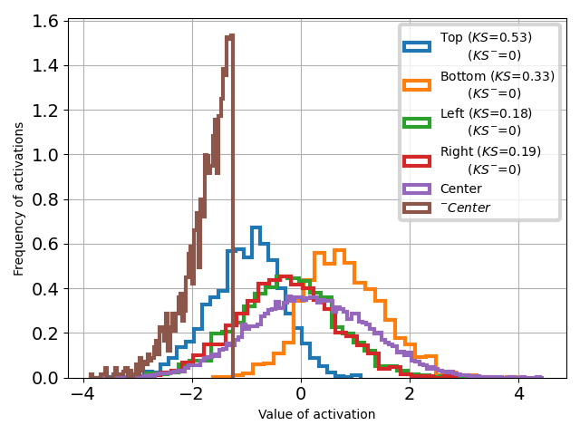
Figure 5: Histogram of neuron activations on the border regions, the center (purple) and the center truncated on the minus side (brown). Legend shows to Kolmogorov-Smirnov test. $KS$ corresponds to border vs center. $KS^{-}$ corresponds to border vs truncated center. Model: ResNet50. Layer: Conv3_2. Neuron idx: 46.

The effect of using the truncated centre PDF, is shown in Figure 5. The plot shows a neuron with negative activations for the top border, with the rest of activations being closer to zero. The computed $KS(A_{top},A_{centre})$ is 0.53. These results indicate this neuron is a vertical edge detector. However, when compared with the truncated $A_{centre}^{-}$, the same $A_{top}$ is no longer distinctive ($KS^{-}(A_{top},A_{centre}^{-})=0.0$), which indicates this neuron is not a PAN.

Given these insights, we label as PANs neurons which hold (1) a high $KS(A_{top|bottom|left|right},A_{centre})$ and, (2) a high $KS^{+}(A_{top|bottom|left|right},A_{centre}^{+})$ or a high $KS^{-}(A_{top|bottom|left|right},A_{centre}^{-})$. We set a threshold $\theta=0.5$ in the rest of the paper. $\theta$ can be modified to reduce or increase the requirements needed for PAN detection. The distributions of PANs identified using this methodology with $\theta=0.5$ is shown in Table 1.

On the models considered and with $\theta=0.5$, PANs represent roughly 2% of all convolutional filters, and can be found at different depths. This may be caused by the explicit information about the presence of padding being lost or integrated (thus mixing with other activations) into other neurons after going through several layers. The disappearance of explicit padding information, however, does not preclude the information being used by the model, but it can motivate the model to periodically re-locate explicit padding so that the next few layers can more easily use that information. Later layers seem to include a remarkable amount of PANs, likely influenced by the large number of neurons found there. This could be influenced by the reduced reliability of the KS method when applied on inputs with small width and height, but it could also indicate padding location plays an important role on the final prediction.

Overall, applying the methodology to thousands of filters yields hundreds of edge detectors and dozens of PANs per model. By slightly weakening the restrictions required to be labelled as a PAN their number can be easily doubled (e.g., ResNet includes 193 PANs when using $\theta=0.4$).

3.3 PAN exploration

Let us analyse neurons identified as PANs by the previously proposed method. For each neuron we look at their histogram of activations for the centre (complete and truncated PDF) and border regions. We also show these same plots, when inference is made replacing the zero padding policy by a reflect padding policy. Finally, we show activation maps for a couple of samples to understand its spatial response.

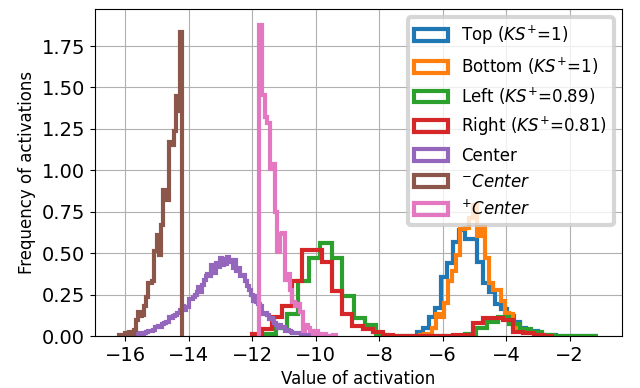
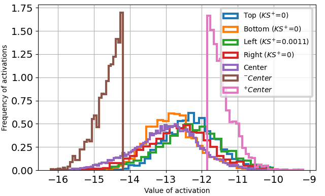
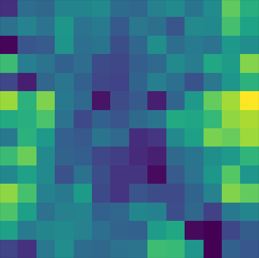
Figure 6: Top plot: Activation histogram of a PAN, where all four borders have high KS. Includes distributions for border regions, and central locations (complete and truncated). Legend shows KS confidence w.r.t. truncated distribution (i.e., $KS^{+}(A_{border},A_{centre}^{+})$). Middle plot: Same as top, using padding reflect. Bottom plots: Activation heatmap on an input with zero and reflect padding. Model: ResNet50. Layer: Conv3_1. Neuron idx: 41.

The top plot of Figure 6 shows a PAN, with distinctively low activation values on all four borders, even when compared against the lowest values produced within the larger central area (i.e., $A_{centre}^{+}$, in pink). With $\theta=0.5$, the PAN is detected as TBLR. An inspection of the activations produced by the kernel on two inputs (bottom plot of Figure 6) shows how this PAN has a preference for the bottom and top padding, which is consistent with $KS^{+}(A_{left|right},A_{centre}^{+})<KS^{+}(A_{top|bottom},A_{centre}^{+})$ (as shown in the top plot). Notice $A_{left}$ and $A_{right}$ have a bimodal distribution, peaking both at -10 and at -4. This is caused by particularly strong activations on corner positions, which are high even within $A_{top}$ and $A_{bottom}$. This neuron, beyond being padding aware, is also corner aware, a behavior found on other neurons (e.g., conv1_0, 17; conv3_1, 212; conv4_1, 296; conv4_2, 447). When the padding is changed from zero to reflect, as shown in the middle plot of Figure 6, the neuron no longer detects padding. The distributions of activation values for border regions become indistinguishable from the distribution in the centre.

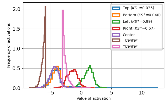
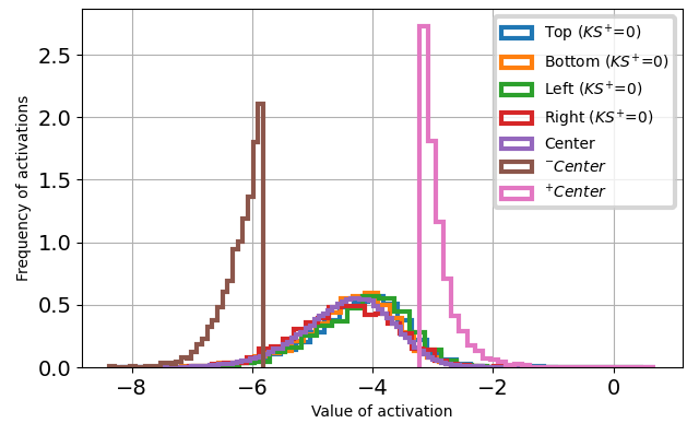
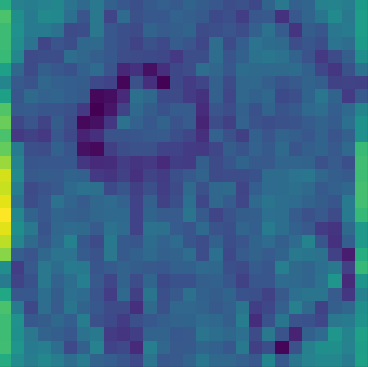
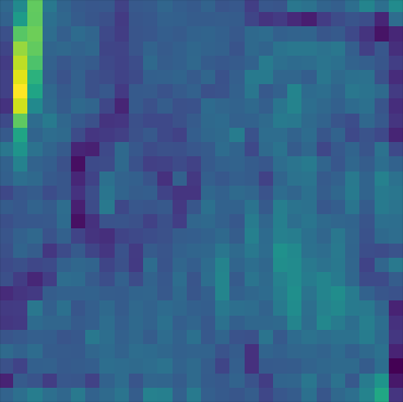
Figure 7: Top plot: Activation histogram of a PAN, where the left and right borders have high KS. Includes distributions for border regions, and central locations (complete and truncated). Legend shows KS confidence w.r.t. truncated distribution (i.e., $KS^{+}(A_{border},A_{centre}^{+})$). Middle plot: Same as top, using padding reflect. Bottom plots: Activation heatmap on an input with zero and reflect padding. Model: ResNet50. Layer: Conv2_1. Neuron idx: 67

Another representative neuron is shown in Figure 7. In this case the PAN activates distinctively high on the left and right padding. Since $A_{left}$ is significantly higher than $A_{right}$, this may be primarily a L PAN that also detects the right border by complement. This is in fact a behaviour compatible with the kernel shown at the centre of Figure 1. For the top and bottom padding locations, this neuron’s activations are indistinguishable from those on central locations. The long tail of the top and bottom distributions speaks of potential corner detection capabilities. All this is illustrated by the bottom plot of Figure 7, which shows activations on two inputs. Notice some edges are detected in centre locations, but not as strongly as on the left and right padding. The middle plot of Figure 7 shows the same activations when zero padding is replaced by reflect padding. When this is the case, the neuron no longer detects padding, with $A_{left}$ and $A_{right}$ becoming aligned with the rest of distributions.

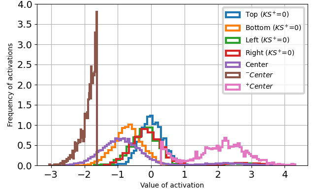
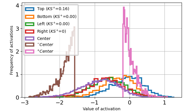
Figure 8: Top plot: Activation histogram of a neuron which is an edge detector candidate and a potential downstream PAN, not detected as PAN. Includes distributions for border regions, and central locations (complete and truncated). Legend shows KS confidence w.r.t. truncated distribution (i.e., $KS^{+}(A_{border},A_{centre}^{+})$). Notice the truncated centre distribution on the high side (pink) is bimodal, with one peak around zero and one around two. Middle plot: Same as top, using padding reflect instead of zero. Bimodal distribution disappears. Bottom plots: Activation heatmap on an input with zero and reflect padding. Model: ResNet50. Layer: Conv3_2. Neuron idx: 158

The last neuron discussed here is the downstream PAN of Figure 8. Following the proposed methodology, this neuron is detected as a potential edge detector ($KS(A_{top},A_{centre})=0.66$), but not as a PAN ($KS^{+}(A_{top},A_{centre})=0.0$) (see top plot). Its spatial activations on two different inputs (bottom plots of Figure 8) indicate this is no regular edge detector. It activates distinctively on the second highest row of the input, as if it was detecting the top padding from afar. This explains the bimodal behaviour of this neuron in the top plot, where the truncated ${}^{+}centre$ distribution (which includes most of the second row) peaks both at around two (activations of the second highest row) and zero (activations on the rest of centre). Since the kernel of this neuron is 3x3, it cannot directly detect the padding from this location (i.e., on the second highest row activations, the kernel is located entirely on the unpadded input). This neuron gets the information about image border location from a previous layer, and turns off (see middle plot of Figure 8) when static padding is removed.

3.4 Nascent PAN types

Through the analysis defined in the previous sections we have characterised and identified several types of nascent PANs, those that directly detect padding in the input. Nascent PANs frequently have a multi-modal behaviour, detecting two or more padding edges. This multi-border detection can be generic (i.e., several borders detected indistinguishably), or it can be distinct for different border types. The neuron shown in Figure 6, for example, can discriminate between horizontal borders (top and bottom), vertical borders (left and right) and the rest of the input. But it cannot discriminate among horizontal borders (between top and bottom padding), or among vertical ones (left and right padding). On the other hand, the neuron shown in Figure 7 can discriminate between left and right padding. This later behaviour is consequence of the asymmetrical kernels PANs may have, exemplified in the kernels of Figure 1.

PAN type	T	B	L	R	TB	TL	TR	BL	BR	LR	TBL	TBR	TLR	BLR	TBLR
ResNet	10	32	8	10	8	1	0	0	3	4	1	0	0	0	4
MobileNet	47	90	9	6	9	5	0	1	3	8	0	0	1	1	13
GoogLeNet	7	24	4	2	7	1	0	0	1	7	0	0	1	1	3

Table 2: Distribution of PAN types identified on different models, with $\theta=0.5$.

We identify 14 possible types of nascent PANs based on which padding borders they detect (i.e., T, B, L, R, TB, TL, TR, BL, BR, LR, TBL, TBR, BLR and TBLR). We study the distribution of nascent PAN types with the proposed method in Table 2. Single border detectors (i.e., T, B, L, R) are the most frequent types, representing about 75% of all identified PANs. The rest are mostly PANs which can detect complementary borders (i.e., TB, LR), or all four borders (i.e., TBLR). Complementary borders detecting PANs are likely to be mirrored variations of the kernel shown in the middle of Figure 1, while the four borders PAN may be asymmetrical versions of the bottom Laplacian of Gaussian filter shown in Figure 2.

4 Performance and Bias

Once we have established the existence and pervasiveness of PANs in models trained with zero padding, let us now assess the role these neurons play in model behaviour. To do so, we study their influence in the network output using four versions of the same pre-trained ResNet50, without fine-tuning:

• The original model, using the default zero-padding.

• The reflect model, where the padding of all convolutional neurons has been changed to PyTorch’s reflect.

• The PAN-reflect model, where the padding of the neurons identified as PANs by the previous methodology (for ResNet50, 2.0% of convolutional neurons, 81 overall) has been changed to reflect. The rest of neurons preserve zero-padding.

• The RAND-reflect model, where the padding of randomly sampled non-PANs has been changed to reflect and the rest preserve zero-padding. The random subset has the same size (2.0% of neurons) and follows the same layer distribution as PAN-reflect. This is the control set.

We use the quantitative differences in the outputs of these models to study the impact padding has towards specific classes (i.e., the amount of padding bias). Then, we study the influence of PANs in the context of particular data samples.

4.1 Bias influence

To verify to which extend PANs add relative location bias to the model, we compare the soft-max outputs of original with those of PAN-reflect. To be precise, we compute the odds of the prediction probability for each class. Assuming samples to be i.i.d., this can be computed as the quotient of the sum of soft-max outputs for all images $i$ in the dataset:

$$Odds(c)=\frac{P(c|M_{Pan-reflect})}{P(c|M_{original})}=\frac{\sum_{i}M_{Pan-reflect}(i)[c]}{\sum_{i}M_{original}(i)[c]}$$

And analogously for RAND-reflect. For PAN-reflect, odds above $1$ for a class $c$ indicate a higher confidence in the prediction of $c$ in the absence of PANs. This can also be interpreted as padding being used as evidence against that class. Conversely, values below $1$ would imply padding is being used as evidence toward the class.

Figure 9 presents the logarithm of the odds per class, computed on the ILSVRC validation set for both PAN-reflect and RAND-reflect. All classes are affected, a few severely so. Table 3 lists all classes whose odds change by more than 7%. We choose a threshold instead of the top-K to illustrate how the odds change in an asymmetrical manner: there are more classes which use padding as evidence toward the class (odds $<$ 1) than those that use it against. Remarkably, classes for which padding is used as evidence against it seem to be mostly fine-grained types (mainly animal species and dogs, with the exception of sliding door), which hints at the relevance of padding for overfitting. Conversely, there are no animals among the classes that use padding as positive evidence. Using a 5% threshold yields consistent results: out of the 111 classes with negative log odds, the only animal is the English Foxhound, whereas for the 99 classes with positive log odds, there are only five classes which are not fine-grained animals.

To verify if findings are related with the relevance of padding or with the noise added by the data distribution, let us consider the results while using RAND-reflect (orange in Figures 9 and 10). In this case, the distribution of PANs’ odds is characteristically different from that of random, similarly-sampled neuron sets. While PANs seem to affect most classes to a large degree, either positively or negatively, the random set effect on classes is very limited. Only a few classes are affected, with the most common result being no output change. These results indicate PANs strongly and homogeneously alter most classes’ prior, whereas an equally sized random subset of neurons does not.

Repeating this experiment with model reflect changes the input distribution of 100% of convolutional layers, whereas the previous two experiments (with PAN-reflect and RAND-reflect) changed only 2% of neurons. As a result, the reflect odds suffer more extreme changes than either one of the above. No tendency around which classes receive positive and which negative log odds was found. In this particular experiment, we believe the larger odds variance has to do with noise added to the distributions, rather than due to some intrinsic quality of how padding is used.

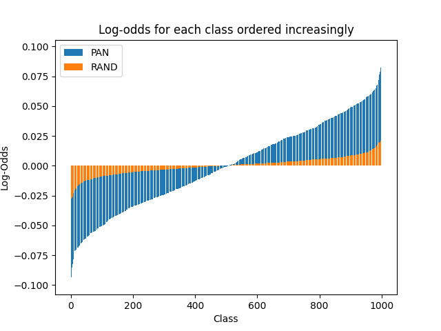
Figure 9: Ordered change in log-odds, for PAN-reflect and RAND-reflect w.r.t. original model. Vertical axis is the amount of change. $\pm 0.05$ log-odds corresponds to 5% difference in odds.

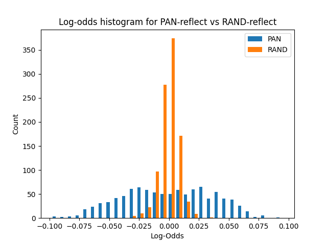
Figure 10: Class histogram of log odds change w.r.t. original model, computed for both PAN-reflect and RAND-reflect. Notice how the former has both a wider range and a bimodal distribution.

Class	Odds	Class	Odds
drum	0.91	cheetah	1.10
muzzle	0.91	Norfolk Terrier	1.09
packet	0.91	sliding door	1.09
sunscreen	0.92	Irish Water Spaniel	1.08
barrette	0.92	box turtle	1.08
tandem bicycle	0.92	Dobermann	1.08
candle	0.92	Flat-Coated Retriever	1.08
tent	0.92	Alaskan Malamute	1.08
tray	0.92	gossamer-winged butterfly	1.07
comic book	0.93	West Highland White Terrier	1.07
Windsor tie	0.93	Greater Swiss Mountain Dog	1.07
tile roof	0.93	guenon	1.07
backpack	0.93
overskirt	0.93
buckle	0.93
lab coat	0.93
shoal	0.93
paper knife	0.93
whistle	0.93
ice pop	0.93
stethoscope	0.93
barbell	0.93
lakeshore	0.93
megalith	0.93
scarf	0.93

Table 3: Classes with odds beyond 7% computed between the PAN-reflect and the original model. Classes with odds above one, increase their confidence in the absence of PAN information, are less frequent and are mostly composed of animals. For odds below 1, we check $\frac{1}{odds(c)}>1.07$.

4.2 Sample influence

The previous section shows a clear influence of padding in the overall performance and behaviour of the model. However, the class-scale at which analysis is made means that the effect of PANs on single predictions is aggregated in the mean for each class. To analyse this facet, we look for the individual samples with the largest change in the network’s output. We compute this change as the Manhattan distance between the logits of the original and the PAN-reflect model.

Significantly, the 30 images with the biggest padding influence are all incorrectly classified by both the original and the PAN-reflect models, the predicted class remaining the same. Analysing the top 5,000 most affected images (10% of the whole dataset), we find that the number of disagreements between models is remarkably low (67 images). The limited impact PANs have on samples which are not part of the model training set, could also be the result of padding information being used for overfitting particularly hard training samples.

When repeating the experiment on RAND-reflect, these effects disappear. The sample with the 5000th highest divergence with the PAN-reflect has around 4 distance units, whereas for RAND-reflect with this distance happens on the 13th sample. This alone shows PAN-reflect affects with more strength to orders of magnitude more samples than RAND-reflect. Of those 13 samples, 12 of them are incorrectly predicted as tench, which indicates the preference of these randomly chosen 2% of neurons for this class.

5 Discussion

The use of static padding in convolutional layers provides the model with a stable signal of a perceptual edge. That much was known from previous works [2, 17, 1, 14]. This paper reveals the extent of this inductive spatial bias, identifying a set of neurons specialized in locating and exploiting it (what we call PANs), which account for at least 1.5%-3% of all deep CNNs convolutional filters. Considering PANs are likely to be inheritable (as long as the fine-tuned model keeps zero padding) and the fact that PANs were found on popular pre-training sources, one can assume PANs are a widespread phenomenon.

Experiments indicate padding information is used to change the prior of most classes. PANs seem to be used as evidence against fine-grained classes (i.e., animals), and seldom as evidence for them. For the ILSVRC task we derive two different hypothesis for explaining this. Either samples from fine-grained class are generally better framed, which keeps the padding away from the patterns most relevant for the class, resulting in a spatial bias that can be leveraged; or padding is used as a reference to identify arbitrary patterns in particularly hard samples, helping overfit on examples from the long tail [5]. Testing both these hypothesis remains future work as it requires its own experimental setup.

The desirability of PANs in a model depends on the application, and its definition of un/desirable bias. On tasks with fixed framing (e.g., fundus retina images [26], static cctv feed [4] etc.) PANs may provide a useful location reference allowing a better contextualisation and structuring of the input. On tasks which entail frame freedom (e.g., objects in the wild, variances among devices) PANs learn an arbitrary bias, which may contribute to overfitting and lack of generalisation [2, 17, 1]. For these reasons, we recommend practitioners to choose padding carefully, using dynamic padding (such as reflect) by default but accounting for the removal of PAN information. It remains to be seen how the presence of PANs affect in downstream tasks different to classification, such as training or fine-tuning for object detection, or whether fine-tuning in a new task removes or adds more PANs.

Even when PANs are useful, their current design is not efficient. A lot of parameters (PAN kernels) and computation are wasted on recognizing a constant. For those cases where PANs are indeed desirable, one may find more efficient and rich versions of them, at least in three different ways: (1) by implementing a sparse computation which skips padding products, (2) by using models with pre-initialised PAN kernels spread along the model, and (3) by adding the complementary axis information to padding (row height in vertical padding and vice-versa) for complete spatial reference.

Finally, let us consider a safety vulnerability PANs entail. Given their characteristic pattern, PANs are easy to fool and trigger. Adding a one-row/column of zeros anywhere in the input will cause PANs to fire, out of the manifold and into unpredictability. This can be easily mitigated, for example, by doing data augmentation during training with random rows/columns of padding in the input. This is strongly suggested for models deployed on critical domains.

6 Acknowledgements

We acknowledge previous collaborations with Carles Garriga and Victor Badenas, trying to locate PANs using kernel values. We would also like to acknowledge Ferran Parés for early discussions in the conceptualization of this work. This work has been partially funded by the project SGR-Cat 2021 HPAI (AGAUR grant n.01187).

References

- [1] Farzin Aghdasi and Rabab K Ward. Reduction of boundary artifacts in image restoration. IEEE Transactions on Image Processing, 5(4):611–618, 1996.
- [2] Bilal Alsallakh, Narine Kokhlikyan, Vivek Miglani, Jun Yuan, and Orion Reblitz-Richardson. Mind the pad–cnns can develop blind spots. arXiv preprint arXiv:2010.02178, 2020.
- [3] Víctor Badenas Crespo. Detection and location of contrast-aware and border-aware neurons in convolutional neural networks. Master’s thesis, Universitat Politècnica de Catalunya, 2022.
- [4] Muhammad Tahir Bhatti, Muhammad Gufran Khan, Masood Aslam, and Muhammad Junaid Fiaz. Weapon detection in real-time cctv videos using deep learning. IEEE Access, 9:34366–34382, 2021.
- [5] Daniel D’souza, Zach Nussbaum, Chirag Agarwal, and Sara Hooker. A tale of two long tails. arXiv preprint arXiv:2107.13098, 2021.
- [6] Li Fei-Fei, Rob Fergus, and Pietro Perona. Learning generative visual models from few training examples: An incremental bayesian approach tested on 101 object categories. In 2004 conference on computer vision and pattern recognition workshop, pages 178–178. IEEE, 2004.
- [7] Kunihiko Fukushima and Sei Miyake. Neocognitron: A self-organizing neural network model for a mechanism of visual pattern recognition. In Competition and cooperation in neural nets, pages 267–285. Springer, 1982.
- [8] Carles Garriga Estradé. Studying the characterization of deep cnn neurons. Master’s thesis, Universitat Politècnica de Catalunya, 2019.
- [9] Charles R. Harris, K. Jarrod Millman, Stéfan J. van der Walt, Ralf Gommers, Pauli Virtanen, David Cournapeau, Eric Wieser, Julian Taylor, Sebastian Berg, Nathaniel J. Smith, Robert Kern, Matti Picus, Stephan Hoyer, Marten H. van Kerkwijk, Matthew Brett, Allan Haldane, Jaime Fernández del Río, Mark Wiebe, Pearu Peterson, Pierre Gérard-Marchant, Kevin Sheppard, Tyler Reddy, Warren Weckesser, Hameer Abbasi, Christoph Gohlke, and Travis E. Oliphant. Array programming with NumPy. Nature, 585(7825):357–362, Sept. 2020.
- [10] Kaiming He, Xiangyu Zhang, Shaoqing Ren, and Jian Sun. Deep residual learning for image recognition. In Proceedings of the IEEE conference on computer vision and pattern recognition, pages 770–778, 2016.
- [11] Andrew Howard, Mark Sandler, Grace Chu, Liang-Chieh Chen, Bo Chen, Mingxing Tan, Weijun Wang, Yukun Zhu, Ruoming Pang, Vijay Vasudevan, et al. Searching for mobilenetv3. In Proceedings of the IEEE/CVF international conference on computer vision, pages 1314–1324, 2019.
- [12] Yu-Hui Huang, Marc Proesmans, and Luc Van Gool. Context-aware padding for semantic segmentation. arXiv preprint arXiv:2109.07854, 2021.
- [13] Fazle Karim, Somshubra Majumdar, Houshang Darabi, and Shun Chen. Lstm fully convolutional networks for time series classification. IEEE access, 6:1662–1669, 2017.
- [14] Osman Semih Kayhan and Jan C van Gemert. On translation invariance in cnns: Convolutional layers can exploit absolute spatial location. In Proceedings of the IEEE/CVF Conference on Computer Vision and Pattern Recognition, pages 14274–14285, 2020.
- [15] Raman Maini and Himanshu Aggarwal. Study and comparison of various image edge detection techniques. International journal of image processing (IJIP), 3(1):1–11, 2009.
- [16] Sébastien Marcel and Yann Rodriguez. Torchvision the machine-vision package of torch. In Proceedings of the international conference on Multimedia - MM ’10, page 1485, Firenze, Italy, 2010. ACM Press.
- [17] Anh-Duc Nguyen, Seonghwa Choi, Woojae Kim, Sewoong Ahn, Jinwoo Kim, and Sanghoon Lee. Distribution padding in convolutional neural networks. In 2019 IEEE International Conference on Image Processing (ICIP), pages 4275–4279. IEEE, 2019.
- [18] Adam Paszke, Sam Gross, Francisco Massa, Adam Lerer, James Bradbury, Gregory Chanan, Trevor Killeen, Zeming Lin, Natalia Gimelshein, Luca Antiga, Alban Desmaison, Andreas Köpf, Edward Yang, Zach DeVito, Martin Raison, Alykhan Tejani, Sasank Chilamkurthy, Benoit Steiner, Lu Fang, Junjie Bai, and Soumith Chintala. PyTorch: An Imperative Style, High-Performance Deep Learning Library. arXiv:1912.01703 [cs, stat], Dec. 2019. arXiv: 1912.01703.
- [19] Robin Rombach, Andreas Blattmann, Dominik Lorenz, Patrick Esser, and Björn Ommer. High-resolution image synthesis with latent diffusion models. In Proceedings of the IEEE/CVF Conference on Computer Vision and Pattern Recognition, pages 10684–10695, 2022.
- [20] Olga Russakovsky, Jia Deng, Hao Su, Jonathan Krause, Sanjeev Satheesh, Sean Ma, Zhiheng Huang, Andrej Karpathy, Aditya Khosla, Michael Bernstein, et al. Imagenet large scale visual recognition challenge. International Journal of Computer Vision, 115(3):211–252, 2015.
- [21] Christian Szegedy, Wei Liu, Yangqing Jia, Pierre Sermanet, Scott Reed, Dragomir Anguelov, Dumitru Erhan, Vincent Vanhoucke, and Andrew Rabinovich. Going deeper with convolutions. In Proceedings of the IEEE conference on computer vision and pattern recognition, pages 1–9, 2015.
- [22] Pauli Virtanen, Ralf Gommers, Travis E. Oliphant, Matt Haberland, Tyler Reddy, David Cournapeau, Evgeni Burovski, Pearu Peterson, Warren Weckesser, Jonathan Bright, Stéfan J. van der Walt, Matthew Brett, Joshua Wilson, K. Jarrod Millman, Nikolay Mayorov, Andrew R. J. Nelson, Eric Jones, Robert Kern, Eric Larson, C J Carey, İlhan Polat, Yu Feng, Eric W. Moore, Jake VanderPlas, Denis Laxalde, Josef Perktold, Robert Cimrman, Ian Henriksen, E. A. Quintero, Charles R. Harris, Anne M. Archibald, Antônio H. Ribeiro, Fabian Pedregosa, Paul van Mulbregt, SciPy 1.0 Contributors, Aditya Vijaykumar, Alessandro Pietro Bardelli, Alex Rothberg, Andreas Hilboll, Andreas Kloeckner, Anthony Scopatz, Antony Lee, Ariel Rokem, C. Nathan Woods, Chad Fulton, Charles Masson, Christian Häggström, Clark Fitzgerald, David A. Nicholson, David R. Hagen, Dmitrii V. Pasechnik, Emanuele Olivetti, Eric Martin, Eric Wieser, Fabrice Silva, Felix Lenders, Florian Wilhelm, G. Young, Gavin A. Price, Gert-Ludwig Ingold, Gregory E. Allen, Gregory R. Lee, Hervé Audren, Irvin Probst, Jörg P. Dietrich, Jacob Silterra, James T Webber, Janko Slavič, Joel Nothman, Johannes Buchner, Johannes Kulick, Johannes L. Schönberger, José Vinícius de Miranda Cardoso, Joscha Reimer, Joseph Harrington, Juan Luis Cano Rodríguez, Juan Nunez-Iglesias, Justin Kuczynski, Kevin Tritz, Martin Thoma, Matthew Newville, Matthias Kümmerer, Maximilian Bolingbroke, Michael Tartre, Mikhail Pak, Nathaniel J. Smith, Nikolai Nowaczyk, Nikolay Shebanov, Oleksandr Pavlyk, Per A. Brodtkorb, Perry Lee, Robert T. McGibbon, Roman Feldbauer, Sam Lewis, Sam Tygier, Scott Sievert, Sebastiano Vigna, Stefan Peterson, Surhud More, Tadeusz Pudlik, Takuya Oshima, Thomas J. Pingel, Thomas P. Robitaille, Thomas Spura, Thouis R. Jones, Tim Cera, Tim Leslie, Tiziano Zito, Tom Krauss, Utkarsh Upadhyay, Yaroslav O. Halchenko, and Yoshiki Vázquez-Baeza. SciPy 1.0: fundamental algorithms for scientific computing in Python. Nature Methods, 17(3):261–272, Mar. 2020.
- [23] Shuang Wu, Guanrui Wang, Pei Tang, Feng Chen, and Luping Shi. Convolution with even-sized kernels and symmetric padding. Advances in Neural Information Processing Systems, 32, 2019.
- [24] Hongming Xu, Cheng Lu, Richard Berendt, Naresh Jha, and Mrinal Mandal. Automatic nuclei detection based on generalized laplacian of gaussian filters. IEEE Journal of Biomedical and Health Informatics, 21(3):826–837, 2017.
- [25] Kun Yuan, Shaopeng Guo, Ziwei Liu, Aojun Zhou, Fengwei Yu, and Wei Wu. Incorporating convolution designs into visual transformers. In Proceedings of the IEEE/CVF International Conference on Computer Vision, pages 579–588, 2021.
- [26] Miguel Angel Zapata, Dídac Royo-Fibla, Octavi Font, José Ignacio Vela, Ivanna Marcantonio, Eduardo Ulises Moya-Sánchez, Abraham Sánchez-Pérez, Dario Garcia-Gasulla, Ulises Cortés, Eduard Ayguadé, et al. Artificial intelligence to identify retinal fundus images, quality validation, laterality evaluation, macular degeneration, and suspected glaucoma. Clinical Ophthalmology (Auckland, NZ), 14:419, 2020.
- [27] Ziqi Zhang, David Robinson, and Jonathan Tepper. Detecting hate speech on twitter using a convolution-gru based deep neural network. In European semantic web conference, pages 745–760. Springer, 2018.