T. Anderson Keller
UvA-Bosch Delta Lab
University of Amsterdam, NL
&Lyle Muller
Department of Mathematics
Western University, CA
&Terrence Sejnowski
Computational Neurobiology Lab
Salk Institute for Biological Studies, USA
&Max Welling
UvA-Bosch Delta Lab
University of Amsterdam, NL
Correspondence: T.Anderson.Keller@gmail.com

Traveling Waves Encode the Recent Past
and Enhance Sequence Learning

T. Anderson Keller
UvA-Bosch Delta Lab
University of Amsterdam, NL
&Lyle Muller
Department of Mathematics
Western University, CA
&Terrence Sejnowski
Computational Neurobiology Lab
Salk Institute for Biological Studies, USA
&Max Welling
UvA-Bosch Delta Lab
University of Amsterdam, NL
Correspondence: T.Anderson.Keller@gmail.com

Abstract

Traveling waves of neural activity have been observed throughout the brain at a diversity of regions and scales; however, their precise computational role is still debated. One physically grounded hypothesis suggests that the cortical sheet may act like a wave-field capable of storing a short-term memory of sequential stimuli through induced waves traveling across the cortical surface. To date, however, the computational implications of this idea have remained hypothetical due to the lack of a simple recurrent neural network architecture capable of exhibiting such waves. In this work, we introduce a model to fill this gap, which we denote the Wave-RNN (wRNN), and demonstrate how both connectivity constraints and initialization play a crucial role in the emergence of wave-like dynamics. We then empirically show how such an architecture indeed efficiently encodes the recent past through a suite of synthetic memory tasks where wRNNs learn faster and perform significantly better than wave-free counterparts. Finally, we explore the implications of this memory storage system on more complex sequence modeling tasks such as sequential image classification and find that wave-based models not only again outperform comparable wave-free RNNs while using significantly fewer parameters, but additionally perform comparably to more complex gated architectures such as LSTMs and GRUs. We conclude with a discussion of the implications of these results for both neuroscience and machine learning.

1 Introduction

Traveling waves have been observed during awake and sleep states throughout the brain, including the cortex and hippocampus, in many frequency bands, and have recently been shown to have a direct impact on behavior in awake behaving primates Davis2020 . Their existence and ubiquity appear to challenge the classical receptive field representation of visual stimuli, which assumes that neurons in cortex carry information that is spatially and temporally localized.

Several computational hypotheses for traveling waves have been suggested, including that they can tag locations in a cortical region with a unique phase ermentrout2001traveling , and that they can aid memory consolidation Muller2016 . A promising hypothesis, derived from the study of physical wave fields perrard2016wave , suggests that traveling waves may serve to efficiently encode recent sequential inputs Muller2018 . To date however, it has been challenging to test these hypotheses due to a lack of standard artificial neural network architectures shown to exhibit such wave-like dynamics.

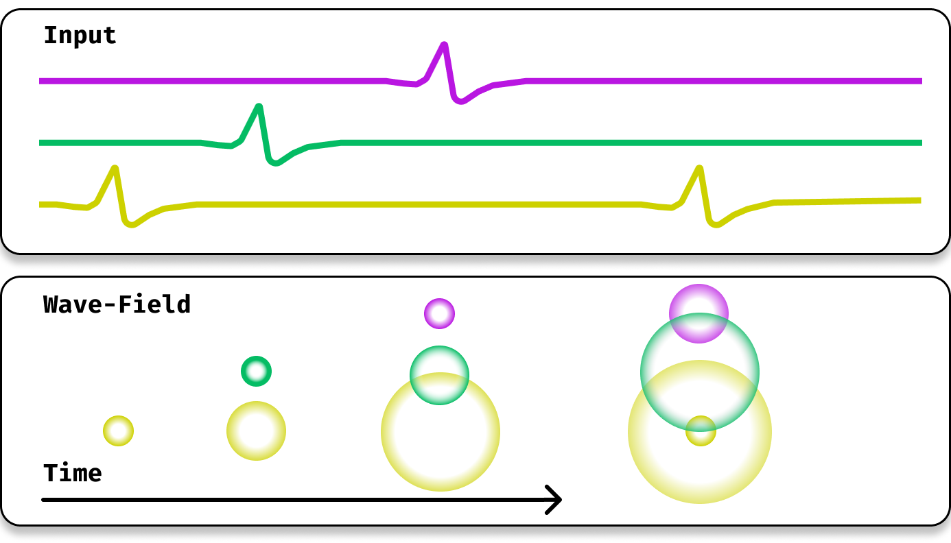
Figure 1: Illustration of three input signals (top) and a corresponding wave-field with induced traveling waves (bottom). From an instantaneous snapshot of the wave-field at each timestep we are able decode both the time of onset and input channel of each input spike. Furthermore, subsequent spikes in the same channel do not overwrite one-another.

Here we introduce a minimal recurrent neural network model that exhibits traveling waves of activity within its latent space and test several computational hypotheses. Specifically, we use a suite of synthetic memory tasks to show that models exhibiting traveling waves can solve these tasks orders of magnitude more quickly, do so more accurately, and are able to handle significantly longer sequences than their matched wave-free counterparts. To measure the extent to which this wave-based memory results in generalized performance benefits beyond pathological synthetic tasks, we test the wRNN on modern long-sequence modeling tasks and show that it indeed outperforms wave-free counterparts and is comparable or better than more complex gated recurrent networks such as LSTMs and GRUs. At its core, our work offers two main contributions: first, a simple recurrent neural network architecture that exhibits traveling waves admissible to computational and neuroscientific investigation in a task-oriented manner; and second, a demonstration that traveling waves efficiently encode the recent past thereby benefiting performance on long-sequence tasks.

2 Traveling Waves in Recurrent Neural Networks

In this section, we outline how to integrate traveling wave dynamics into a simple recurrent neural network architecture and provide preliminary analysis of the emergent waves.

Simple Recurrent Neural Networks. As mentioned, the primary goal of this work is to analyze the computational implications of traveling wave dynamics on artificial neural network architectures. In order to reduce potential confounders in this analysis, we strive to study the simplest possible architecture which exhibits traveling waves in its hidden state. To accomplish this, we start with a simple recurrent neural network also known as an Elman Network Elman1990 and consider how we may define its recurrence in order to bias its hidden dynamics towards a simple wave equation. For an input sequence $\{\mathbf{x}_{t}\}_{t=0}^{T}$ with $\mathbf{x}_{t}\in\mathbb{R}^{d}$, and hidden state $\mathbf{h}_{0}=\mathbf{0}$ & $\mathbf{h}_{t}\in\mathbb{R}^{n}$, a simple RNN (sRNN) is defined with the following recurrence:

$$\mathbf{h}_{t+1}=\sigma(\mathbf{U}\mathbf{h}_{t}+\mathbf{V}\mathbf{x}_{t}+\mathbf{b})$$ (1)

In such a model, the input encoder and recurrent connections are both linear, i.e. $\mathbf{V}\in\mathbb{R}^{n\times d}$ and $\mathbf{U}\in\mathbb{R}^{n\times n}$, where $n$ is the hidden state dimensionality and $\sigma$ is a nonlinearity. The output of the network is then given by another linear map of the final hidden state: $\mathbf{y}=\mathbf{W}\mathbf{h_{T}}$, with $\mathbf{W}\in\mathbb{R}^{o\times n}$.

Discrete Traveling Waves. To understand our goal for the time-dynamics of $\mathbf{h}$, we start with the simplest equation which defines our desired dynamics, the one-dimensional one-way wave equation:

$$\frac{\partial h(x,t)}{\partial t}=\nu\frac{\partial h(x,t)}{\partial x}$$ (2)

Where $t$ is our time coordinate, and $x$ defines the continuous spatial coordinate of our hidden state. Since we wish these waves to propagate through an artificial neural network with discrete neurons and discrete timesteps, we first must discretize Equation 2 in both space and time. If we define our hidden neurons to be laid out on a one-dimensional line at regular intervals, we see that the neuron at location $x$, i.e. $h(x,t)$ is equivalent to the $x$’th neuron: $h^{x}_{t}$. In practice, we define our neurons to be arranged in a one-dimensional circle ($S^{1}$) to avoid boundary effects. Then, if we assume a velocity $\nu=1$, we see that we can write a discretization of this equation for small $\Delta t$ as: $h^{x}_{t+\Delta t}=h^{x+\Delta x}_{t}$. In matrix form, this is equivalent to multiplication of the hidden state vector with a circular shift matrix:

$$\mathbf{h}_{t+1}=\Sigma\mathbf{h}_{t}\hskip 14.22636pt\textrm{where}\hskip 14.22636pt\Sigma=\begin{bmatrix}0&1&0&0&\cdots&0\\ 0&0&1&0&\cdots&0\\ 0&0&0&1&\cdots&0\\ \vdots&\vdots&\vdots&\vdots&\ddots&\vdots\\ 0&0&0&0&\cdots&1\\ 1&0&0&0&\cdots&0\\ \end{bmatrix}$$ (3)

We thus see that starting from the sRNN in Equation 1, there are three components we need to consider to reach solutions approaching Equation 3: the activation function $\sigma$, the recurrent connectivity $\mathbf{U}$ and proper initialization. In the following we will outline the choices for each which ultimately define what we call the Wave-RNN (wRNN).

Activation Functions.

Common choices for recurrent neural network activation functions include logistic functions (sigmoid), hyperbolic tangent functions (tanh), and rectified linear functions (ReLU). Prior work studying simple recurrent neural networks has found that linear and rectified linear activations have theoretical and empirical benefits for long-sequence modeling le2015simple ; orvieto2023resurrecting . In this work, we define $\sigma=\textrm{ReLU}$ in order to align with Equation 3 and this prior work. Empirically we also find this to be significantly more performant than $\sigma=\mathrm{tanh}$.

Recurrent Connectivity.

In pursuit of the goal of equating equations 1 and 3, we see that defining the matrix $\mathbf{U}$ to be a randomly initialized dense matrix is likely to be detrimental to the emergence of waves given the desired diagonal structure of $\Sigma$. However, a common linear operator which has a very similar diagonal structure to $\Sigma$ is the convolution operation. Specifically, assuming a single input channel, and a length $3$ convolutional kernel $\mathbf{u}=\left[0,0,1\right]$, we see the following equivalence:

$$\mathbf{u}\star\mathbf{h}_{t-1}=\Sigma\mathbf{h}_{t-1}$$ (4)

where $\star$ defines circular convolution over the hidden state dimensions $n$. In practice we find that increasing the number of channels helps the model to learn significantly faster and reach lower error. To do this, we define $\mathbf{u}\in\mathbb{R}^{c\times c\times f}$ where $c$ is the number of channels, and $f$ is the kernel size, and we reshape the hidden state from a single $n$ dimensional circle to $c$ separate $n^{\prime}=\lfloor\frac{n}{c}\rfloor$ dimensional circular channels (e.g. $\mathbf{h}\in\mathbb{R}^{c\times n^{\prime}}$). We can then write the full recurrence as:

$$\mathbf{h}_{t+1}=\sigma(\mathbf{u}\star\mathbf{h}_{t}+\mathbf{V}\mathbf{x}_{t}+\mathbf{b})$$ (5)

where $\mathbf{V}\mathbf{x}_{t}$ is similarly reshaped to match the channel structure of $\mathbf{h}$.

Initialization.

Finally, similar to the prior work with recurrent neural networks le2015simple ; gu2022efficiently , we find careful choice of initialization can be crucial for the model to converge more quickly and reach lower final error. Specifically, we initialize the convolution kernel such that the matrix form of the convolution (known as a Toeplitz matrix) is exactly that of the shift matrix $\Sigma$ for each channel separately. Succinctly, in the PyTorch framework pytorch , this initialization can be implemented as:

⬇

1 # Shift initalization for U

2 U = torch.zeros(size=(c, c, kernel_size))

3 torch.nn.init.dirac_(U)

4 U = torch.roll(input=U, shifts=1, dims=-1)

Furthermore, we find that initializing the matrix $\mathbf{V}$ to be zero with a single identity mapping from the input to a single hidden unit to further drastically improve training speed. Again, explicitly:

⬇

1 # Sparse identity initialization for V

2 V = torch.zeros(size=(n_hidden, n_input))

3 v = V.view(n_channels, n_hidden // n_channels, n_inp)

4 v[:, 0] = 1.0

Intuitively, these initalizations combined can be seen to support a separate traveling wave of activity in each channel, driven by the input at a single source location.

Wave Recurrent Neural Networks. Combining the above ReLU activation function, convolutional recurrent connections, and specific initalizations, we reach our definition of the Wave-RNN. We note that these are not the only choices which lead to wave-dynamics in the hidden state, however empirically we find them to be the most performant and also the most conducive to wave activity. At the end of Section 3, we empirically demonstrate this through a range of ablation experiments.

Baselines.

In order to isolate the effect of traveling waves on model performance, we desire to pick baseline models which are as similar to the Wave-RNN as possible while not exhibiting traveling waves in their hidden state. To accomplish this, we rely on the Identity Recurrent Neural Network (iRNN) of Le et al. (2015) le2015simple . This model is nearly identical to the Wave-RNN, constructed as a simple RNN with $\sigma=\mathrm{ReLU}$, but uses an identity initialization for $\mathbf{U}$. Despite its simplicity the iRNN is found to be comparable to LSTM networks on standard benchmarks, and thus represents the ideal highly capable simple recurrent neural network which is comparable to the Wave-RNN.

Analysis of Traveling Waves. Before we study the memory and sequence modeling capabilities of the proposed architecture, we first demonstrate that the model does indeed produce traveling waves within its hidden state. To do this, in Figure 2, for the best performing (wRNN & iRNN) models on the Sequential MNIST task of the proceeding section, we plot in the top row the activations of our neurons (vertical axis) over time (horizontal axis) as the RNNs process a sequence of inputs (MNIST pixels). As can be seen, there are distinct diagonal bands of activation for the Wave-RNN (left), corresponding to waves of activity propagating between hidden neurons over time. For the baseline simple RNN (iRNN) right, no such bands exist, but instead stationary bumps of activity exist for durations of time and then fade. In the bottom row, following the analysis techniques of Davis et al. (2021) Davis2021 , we plot the corresponding 2D Fourier transform of the above activation time series. In this plot, the vertical axis corresponds to spatial frequencies while the horizontal axis corresponds to the usual temporal frequencies. In such a 2D frequency space, a constant speed traveling wave (or general moving object Cagigal1995 ) will appear as a linear correlation between spatial and time frequencies. Specifically, the slope of that correlation will then correspond to the speed. Indeed, for the wave RNN, we see a strong band of energy along the diagonal corresponding to our traveling waves with velocity $\approx 0.3\ \frac{\textrm{units}}{\textrm{timestep}}$; as expected, for the iRNN we see no such diagonal band in frequency space.

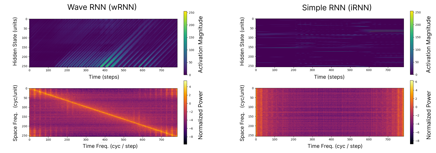
Figure 2: Visualization of hidden state (top) and associated 2D Fourier transform (bottom) for a wRNN (left) and iRNN (right) operating on the sMNIST task. We see the Wave-RNN exhibits a clear flow of activity across the hidden state (diagonal bands) while the iRNN does not.

3 Experiments

In this section we aim to leverage the model introduced in Section 2 to test the computational hypothesis that traveling waves may serve as a mechanism to encode the recent past in a wave-field short-term memory. To do this, we first leverage a suite of frequently used synthetic memory tasks designed to precisely measure the ability of sequence models to store information and learn dependencies over variable length timescales. Following this, we use a suite of standard sequence modeling benchmarks to measure if the demonstrated short-term memory benefits of wRNNs persist in a more complex regime. For each task we perform a grid search over learning rates, learning rate schedules, and gradient clip magnitudes, presenting the best performing models from each category on a held-out validation set in the figures and tables. In the appendix we include the full ranges of each grid search as well as exact hyperparameters for the best performing models in each category.

Copy Task. As a first analysis of the impact of traveling waves on memory encoding, we measure the performance of the wRNN on the standard ‘copy task’, as frequently employed in prior work graves2014neural ; arjovsky2016unitary ; gu2020improving ; henaff2017recurrent . The task is constructed of sequences of categorical inputs of length $T+20$ where the first $10$ elements are randomly chosen one-hot vectors representing a category in $\{1,\ldots 8\}$. The following $T$ tokens are set to category $0$, and form the time duration where the network must hold the information in memory. The next token is set to $9$, representing a delimiter, signaling the RNN to begin reproducing the stored memory as output, and the final $9$ tokens are again set to category $0$. The target for this task is another categorical sequence of length $T+20$ with all elements set to category $0$ except for the last $10$ elements containing the initial random sequence of the input to be reproduced. At a high level, this task tests the ability for a network to encode categorical information and maintain it in memory for $T$ timesteps before eventually reproducing it. Given the hypothesis that traveling waves may serve to encode information in an effective ‘register’, we hypothesize that wave-RNNs should perform significantly better on this task than the standard RNN. For each sequence length we compare wRNNs with 100 hidden units and 6 channels $(n=100,c=6)$ with two baselines: iRNNs of comparable parameter counts $(n=100\Rightarrow 12\textrm{k}\ \textrm{params.})$, and iRNNs with comparable numbers of activations $(n=625)$ but a significantly greater parameter count $(\Rightarrow 403\textrm{k}\ \textrm{params.})$.

In Figure 3, we show the performance of the best performing baseline RNNs and wRNNs, obtained from our grid search, for $T=\{0,30,80\}$. We see that the wRNNs achieve more than 5 orders of magnitude lower loss and learn significantly faster for all sequence lengths. From the visualizatioon of the model outputs in Figure 4, we see that the iRNN has trouble holding items in memory for longer than 10 timesteps, while the comparable wRNN has no problem copying data for up to 500 timesteps.

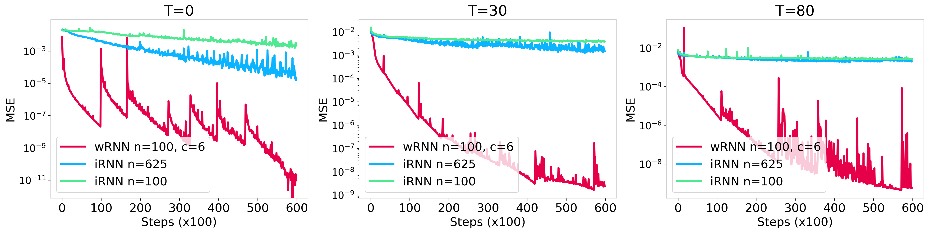
Figure 3: Copy task with lengths T={0, 30, 80}. wRNNs achieve $>$ 5 orders of magnitude lower loss.

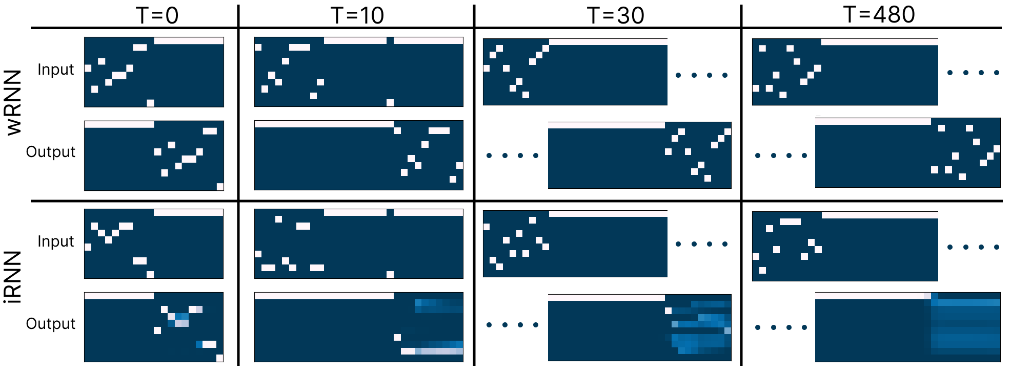
Figure 4: Examples from the copy task for wRNN (n=100, c=6) and iRNN (n=100). We see the iRNN loses significant accuracy after T=10 while the wRNN remains perfect at T=480 ($\mathrm{MSE}\approx 10^{-9}$).

Adding Task. To bolster our findings from the copy task, we employ the long-sequence addition task originally introduced by Hochreiter & Schmidhuber (1997) lstm . The task consists of a two dimensional input sequence of length $T$, where the first dimension is a random sample from $\mathcal{U}([0,1])$, and the second dimension contains only two non-zero elements (set to $1$) in the first and second halves of the sequence respectively. The target is the sum of the two elements in the first dimension which correspond to the non-zero indicators in the second dimension. Similar to the copy task, this task allows us to vary the sequence length and measure the limits of each models ability.

The original iRNN paper le2015simple demonstrated that standard RNNs without identity initialization struggle to solve sequences with $T>150$, while the iRNN is able to perform equally as well as an LSTM, but begins to struggle with sequences of length greater than 400 (a result which we reconfirm here). In our experiments depicted in Figure 5 and Table 1, we find that the wRNN not only solves the task much more quickly than the iRNN, but it is also able solve significantly longer sequences than the iRNN (up to 1000 steps). In these experiments we use an iRNN with $n=100$ hidden units ($10.3$k parameters) and a wRNN with $n=100$ hidden units and $c=27$ channels ($10.29$k parameters).

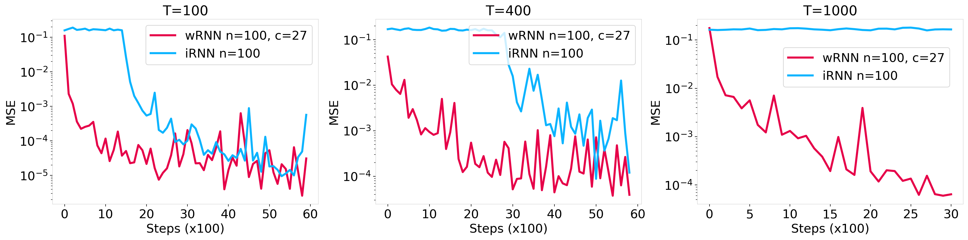
Figure 5: wRNN and iRNN Training curves on the addition task for three different sequence lengths (100, 400, 1000). We see that the wRNN converges significantly faster than the iRNN on all lengths, achieves lower error, and can solve tasks which are significantly longer.

	Seq. Length (T)	100	200	400	700	1000
iRNN	Test MSE	$1\times 10^{-5}$	$4\times 10^{-5}$	$1\times 10^{-4}$	$0.16$	$0.16$
	Solved Iter	14k	22k	30k	$\times$	$\times$
wRNN	Test MSE	$\mathbf{4\times 10^{-6}}$	$\mathbf{2\times 10^{-5}}$	$\mathbf{4\times 10^{-5}}$	$\mathbf{8\times 10^{-5}}$	$\mathbf{6\times 10^{-5}}$
	Solved Iter.	300	1k	1k	3k	2k

Table 1: Long sequence addition task for different sequence lengths. The wRNN finds the task solution (defined as MSE $\leq 5\times 10^{-2}$) multiple orders of magnitude quicker and is able to solve much longer tasks than the iRNN. The $\times$ indicates the model never solved the task after 60k iterations.

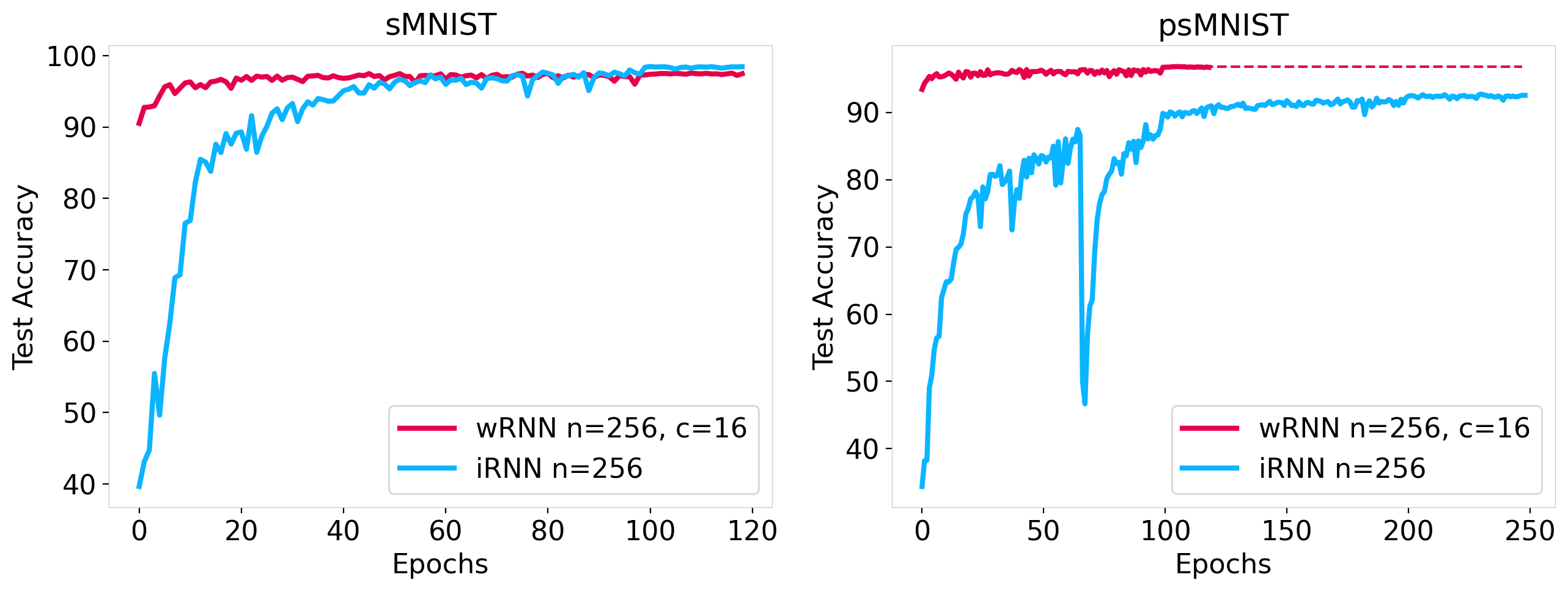
Figure 6: sMNIST (left) and psMNIST (right) training curves for the iRNN & wRNN. The wRNN trains much faster and is virtually unaffected by the sequence permutation, while the iRNN suffers.

Sequential Image Classification.

Given the dramatic benefits that traveling waves appear to afford in the synthetic memory-specific tasks, in this section we additionally strive to measure if waves will have any similar benefits for more complex sequence tasks relevant to the machine learning community. One common task for evaluating sequence models is sequential pixel-by-pixel image classification. In this work we specifically experiment with three sequential image tasks: sequential MNIST (sMNIST), permuted sequential MNIST (psMNIST), and noisy sequential CIFAR10 (nsCIFAR10). The MNSIT tasks are constructed by feeding the 784 pixels of each image of the MNIST dataset one at a time to the RNN, and attempting to classify the digit from the hidden state after the final timestep. The permuted variant applies a random fixed permutation to the order of the pixels before training, thereby increasing the task difficulty by preventing the model from leveraging statistical correlations between nearby pixels. The nsCIFAR10 task is constructed by feeding each row of the image ($32\times 3$ pixels) flattened as vector input to the network at each timestep. This presents a significantly higher input-dimensionality than the MNIST tasks, and additionally contains more complicated sequence dependencies due to the more complex images. To further increase the difficulty of the task, the sequence length is padded from the original length (32), to a length of 1000 with random noise. Therefore, the task of the model is not only to integrate the information from the original 32 sequence elements, but additionally ignore the remaining noise elements. As in the synthetic tasks, we again perform a grid search over learning rates, learning rate schedules, and gradient clip magnitudes. Because of our significant tuning efforts, we find that our baseline iRNN results are significantly higher than those presented in the original work ($98.5\%$ vs. $97\%$ on sMNIST, $91\%$ vs. $81\%$ on psMNIST), and additionally sometimes higher than many ‘state of the art’ methods published after the original iRNN. In the tables below we indicate results from the original work by a citation next to the model name, and lightly shade the rows of our results.

Model	sMNIST	psMNIST	$n$ / $\#\theta$
uRNN arjovsky2016unitary	95.1	91.4	512 / 9k
iRNN	98.5	92.5	256 / 68k
LSTM LEM	98.8	92.9	256 / 267k
GRU LEM	99.1	94.1	256 / 201k
IndRNN (6L) li2018independently	99.0	96.0	128 / 83k
Lip. RNN erichson2021lipschitz	99.4	96.3	128 / 34k
coRNN cornn	99.3	96.6	128 / 34k
LEM LEM	99.5	96.6	128 / 68k
wRNN (16c)	97.6	96.7	256 / 47k
URLSTM gu2020improving	99.2	97.6	1024 / 4.5M
wRNN + MLP	97.5	97.6	256 / 420k
pLMU chilkuri2021parallelizing	-	98.5	468 / 165k
FlexTCN romero2022flexconv	99.6	98.63	- / 375k

Table 2: sMNIST & psMNIST (sorted) test accuracy.

In Table 2, we show our results in comparison with existing work on the sMNIST and psMNIST. Despite the simplicity of our proposed approach, we see that it performs favorably with many carefully crafted RNN and convolutional architectures. We additionally include $\mathrm{wRNN+MLP}$, which is the same as the existing wRNN, but replaces the output map $\mathbf{W}$ with a 2-layer MLP. We see this increases performance significantly, suggesting the linear decoder of the basic wRNN may be a performance bottleneck. In Figure 6 (left), we plot the training accuracy of the best performing wRNN compared with the best performing iRNN over training iterations on the sMNIST dataset. We see that while the iRNN reaches a slightly higher final accuracy (+0.9%), the wRNN trains remarkably faster at the beginning of training, taking the iRNN roughly 50 epochs to catch up. On the right of the figure, we plot the models’ performance on the permuted variant of the task (psMNIST) and see the performance of the Wave-RNN is virtually unaffected, while the simple RNN baseline suffers dramatically.

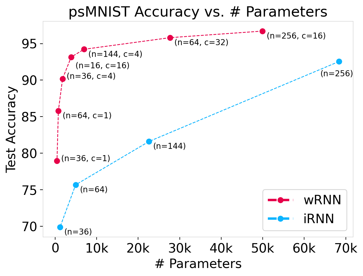
Figure 7: Number of parameters vs. accuracy for wRNNs & iRNNs on psMNIST, attained by varying hidden state size ($n$) and number of channels ($c$). We see that the wRNN achieves significantly higher accuracy at all levels of parameter counts.

We note that in addition to faster training and higher accuracy, the wRNN model additionally exhibits substantially greater parameter efficiency than the iRNN due to its convolutional recurrent connections in place of fully connected layers. To exemplify this, in Figure 7 we show the accuracy (y-axis) of a suite of wRNN models plotted as a function of the number of parameters (x-axis). We see that compared with the iRNN, the wRNN reaches near maximal performance with significantly fewer parameters, and retains a performance gap over the iRNN with increased parameter counts.

Finally, to see if the benefits of the wRNN extend to more complicated images, we explore the noisy sequential CIFAR10 task. In Figure 8 we plot the training curves of the best performing models on this dataset, and see that the Wave-RNN still maintains a significant advantage over the iRNN in this setting. In Table 3, we see the performance of the wRNN is ahead of standard gated architectures such as GRUs and LSTMs, but also ahead of more recent complex gated architectures such as the Gated anti-symmetric RNN chang2019antisymmetricrnn . We note that the parameter count for the wRNN on this task is significantly higher than the other models listed in the table. This is primarily due to the linear encoder mapping from the high dimensionality of the input (96) to the large hidden state. In fact, for this model, the encoder $\mathbf{V}$ alone accounts for $>90\%$ of the parameters of the full model (393k/435k). If one were to replace this encoder with a more parameter efficient encoder, such as a convolutional neural network or a sparse matrix (inspired by the initialization for $\mathbf{V}$), the model would thus have significantly fewer parameters, making it again comparable to state of the art. We leave this addition to future work, but believe it to be one of the most promising approaches to improving the wRNN’s general competitiveness. Ultimately, we see that the wRNN performance is significantly improved over the matched wave-free model. Furthermore, we see that it is surprisingly competitive with state of the art long-sequence models despite having no imposed long-term memory inductive biases besides wave-propagation. We believe that these results therefore serve as strong evidence in support of the hypothesis that traveling waves may be a valuable inductive bias for encoding the recent past and thereby facilitate long-sequence learning.

Figure 8: Training curves for the noisy sequential CIFAR10 dataset.

Model	Acc.	# units / params
LSTM LEM	11.6	128 / 116k
GRU LEM	43.8	128 / 88k
anti-sym. RNN chang2019antisymmetricrnn	48.3	256 / 36k
iRNN	51.3	529 / 336k
Incremental RNN kag2019rnns	54.5	128 / 12k
Gated anti-sym. RNN chang2019antisymmetricrnn	54.7	256 / 37k
wRNN (16c)	55.0	256 / 435k
Lipschits RNN erichson2021lipschitz	57.4	128 / 46k
coRNN cornn	59.0	128 / 46k
LEM LEM	60.5	128 / 116k

Table 3: Test set accuracy on the noisy sequential CIFAR dataset sorted by performance.

Ablation Experiments.

In this section we include a final set of ablation experiments to validate the architecture choices for the Wave-RNN and provide further evidence for the hypothesis that traveling waves are a beneficial inductive bias for sequence learning. For each of the results reported below, a grid search over learning rates, activation functions, initalizations, and gradient clipping values was again performed to ensure fair comparison.

In Table 4, we show the performance of the wRNN on the copy task as we ablate various proposed components such as convolution, $\mathbf{u}$-shift initialization, and $\mathbf{V}$ initialization (as described in Section 2). At a high level, we see that the the $\mathbf{u}$-shift initialization has the biggest impact on performance, allowing the model to successfully solve tasks greater than length $T=10$. We find the $\mathbf{V}$ initialization to be slightly less impactful, improving final performance only marginally, but mainly significantlly increasing the speed of convergence of models (not pictured). In addition to ablating the wRNN, we additionally explore initializing the iRNN with a shift initialization $(\mathbf{U}=\Sigma)$ and sparse identity initialization for $\mathbf{V}$ to disassociate these effects from the effect of the convolution operation. We see that the addition of $\Sigma$ initialization to the iRNN improves its performance dramatically, but it never reaches the same level of performance of the wRNN – indicating that the sparsity and tied weights of the convolution operation are critical to memory storage and retrieval on this task.

Model	Sequence Length (T)
	0	10	30	80
wRNN	$\mathbf{9\times 10^{-12}}$	$\underline{1\times 10^{-10}}$	$\mathbf{8\times 10^{-11}}$	$\mathbf{1\times 8^{-11}}$
- $\mathbf{V}$-init	$\underline{1\times 10^{-11}}$	$\mathbf{2\times 10^{-11}}$	$\underline{4\times 10^{-10}}$	$\underline{4\times 10^{-11}}$
- $\mathbf{u}$-shift-init	$5\times 10^{-11}$	$3\times 10^{-10}$	$7\times 10^{-4}$	$6\times 10^{-4}$
- $\mathbf{V}$-init - $\mathbf{u}$-shift-init	$8\times 10^{-10}$	$1\times 10^{-4}$	$3\times 10^{-4}$	$7\times 10^{-4}$
iRNN (n=100)	$1\times 10^{-4}$	$3\times 10^{-3}$	$2\times 10^{-3}$	$1\times 10^{-3}$
+ $\Sigma$-init	$1\times 10^{-8}$	$1\times 10^{-7}$	$2\times 10^{-7}$	$2\times 10^{-5}$
+ $\Sigma$-init + $\mathbf{V}$-init	$1\times 10^{-7}$	$1\times 10^{-7}$	$1\times 10^{-6}$	$8\times 10^{-6}$

Table 4: Ablation test results (MSE) on the copy task. Best results are bold, second best underlined.

One particularly interesting finding from our ablation studies is that although models without shift initialization do not initially exhibit traveling waves, most randomly initialized models that do learn to perform well on the task eventually learn to exhibit waves in their hidden state. In Figure 9 we show the activation sequence for a wRNN model after initializing kernels with the random Kaming Uniform initialization he2015delving , and then training on the sMNIST task. We see that early in training (left) the model does not exhibit traveling waves; however, by the end of training (right), the randomly initialized model has learned to exhibit waves, and ultimately achieves higher test accuracy than a comparable identity initialized model which never learns to exhibit waves (96.5% vs. 94.8%, training curves in appendix). In the appendix, we include additional ablation studies removing weight sharing in the convolutional layer, and freezing $\mathbf{U}$ & $\mathbf{V}$ at initialization, demonstrating the robustness of traveling waves in these models and providing further support for our empirical conclusions.

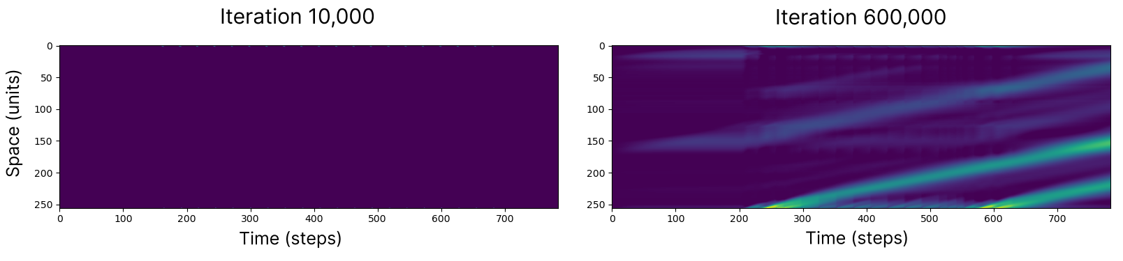
Figure 9: Visualization of the hidden state for a wRNN with randomly initalized kernels (Kaming Uniform). We see the model learns to exhibit traveling waves in its hidden state through training.

4 Discussion

In this section we include a preliminary discussion of related work with a more complete overview in the appendix. Most related to this work in practice, Keller and Welling (2023) nwm showed that an RNN parameterized as a network of locally coupled oscillators similarly exhibits traveling waves in its hidden state, and that these waves served as a bias towards learning structured representations. This present paper introduces a more minimal model capable of producing traveling waves, and thereby permits the study of the direct implications of traveling wave dynamics compared with non-wave models on standard sequence modeling benchmarks. Because our model is a standard simple RNN, the experimental conclusions resulting from the wave dynamics may generalize to more complex state of the art architectures and similarly enhance their performance.

Chen et al. (2022) Chen2022 demonstrated that in a predictive RNN autoencoder learning sequences, a Toeplitz connectivity emerges spontaneously, replicating multiple canonical neuroscientific measurements such as one-shot learning and place cell phase precession. Our results in Figure 9 further support these findings that with proper training and connectivity constraints, recurrent neural networks can learn to exhibit traveling wave activity in service of solving a task.

In another related paper, Benigno et al. (2022) Benigno2022 studied a complex-valued recurrent neural network with distance-dependant connectivity and signal-propagation time-delay, in order to understand the potential computational role for traveling waves that have been observed in visual cortex. They showed that when recurrent strengths are set optimally, the network is able to perform long-term closed-loop video forecasting significantly better than networks lacking this spatially-organized recurrence. Our model is complimentary to this approach, focusing instead on the sequence integration capabilities of waves, rather than on forecasting, and leveraging a more traditional deep learning architecture.

Limitations & Future Work.

The experiments in this paper are inherently limited due to the relatively small scale of the datasets and models studied. For example, nearly all models in this work rely on linear encoders and decoders, and consist of a single RNN layer. Compared with sate of the art models consisting of more complex deep RNNs with skip connections and regularization, our work is therefore potentially leaving significant performance on the table. However, as described above, beginning with small scale experiments on standard architectures yields alternative benefits including more accurate hyperparameter tuning (due to a smaller search space) and potentially greater generality of conclusions. In future work, we plan to test the full implications of our results for the machine learning community and integrate the core concepts from the wRNN into more modern sequence learning algorithms, such as those used for language modeling.

A limitation of our model specifically is the increased number of activations when using a large number of channels. Succinctly, the wRNN requires more memory than the iRNN model in order to store the larger hidden state over time. This limitation can be partially ameliorated by using an adjoint method in the backwards pass so that hidden states can be recomputed when needed and not stored for intermediate steps neuralODE . In preliminary experiments we find that such an approach indeed works and produces waves, offering a suggestion for scaling such models to larger sizes.

Finally, we believe this work opens the door for significant future work in the domains of theoretical and computational neuroscience. For example, direct comparison of the wave properties of our model with neurological recordings may provide novel insights into the mechanisms and role of traveling waves in the brain, analogous to how comparison of visual stream recordings with convolutional neural network activations has yielded insights into the biological visual system dicarlo2014 .

Appendix A Related Work

Deep neural network architectures that exhibit some brain-like properties are related to ours: CORnet [25], a shallow convolutional network with added layer-wise recurrence shown to be a better match to primate neural responses; models with topographic organization, such as the TVAE [23] and TDANN [27]; and models of hippocampal-cortex interactions such as the PredRAE [8], and the TEM [42]. Our work is unique in this space in that it is specifically focused on generating spatio-temporally synchronous activity, unlike prior work. Furthermore, we believe that our findings and approach may be complimentary to existing models, increasing their ability to model neural dynamics by inclusion of the Wave-RNN fundamentals such as locally recurrent connections and shift initalizations.

In the machine learning literature, there are a number of works which have experimented with local connectivity in recurrent neural networks. Some of the earliest examples include Neural GPUs [43] and Convolutional LSTM Networks [40]. These works found that using convolutional recurrent connections could be beneficial for learning algorithms and spatial sequence modeling respectively. Unlike these works however, the present paper explicitly focuses on the emergence of wave-like dynamics in the hidden state, and further studies how these dynamics impact computation. To accomplish this, we also focus on simple recurrent neural networks as opposed to the gated architectures of prior work – providing a less obfuscated signal as to the computational role of wave-like dynamics.

One line of work that is highly related in terms of application is the suite of models developed to increase the ability of recurrent neural networks to learn long time dependencies. This includes models such as Unitary RNNs [1], Orthogonal RNNs [20], expRNNs [28], the chronoLSTM [41], anti.symmetric RNNs [6], Lipschitz RNNs [13], coRNNs [36], unicoRNNs [37], LEMs [38], Recurrent Linear Units [32], and Structured State Space Models (S4) [17]. Additional models with external memory may also be considered in this category such as Neural Turing Machines [15], the DNC [16], memory augmented neural networks [39] and Fast-weight RNNs [2]. Although we leverage many of the benchmarks and synthetic tasks from these works in order to test our model, we note that our work is not intended to compete with state of the art on the tasks and thus we do not compare directly with all of the above models. Instead, the present papers intends to perform a rigorous empirical study of the computational implications of traveling waves in RNNs. To best perform this analysis, we find it most beneficial to compare directly with as similar of a model as possible which does not exhibit traveling waves, namely the iRNN. We do highlight, however, that despite being distinct from aforementioned models algorithmically, and arguably significantly simpler in terms of concept and implementation, the wRNN achieves highly competitive results. Finally, distinct from much of this prior work (except for the coRNN [36]), our work uniquely leverages neuroscientific inspiration to solve the long-sequence memory problem, thereby potentially offering insights into neuroscience observations in return.

Appendix B Experiment Details

In this section, we include all experiment details including the grid search ranges and the best performing parameters. All code for reproducing the results can be found at the following repository: https://github.com/Anon-NeurIPS-2023/Wave-RNN. The code was based on the original code base from the coRNN paper [36] found at https://github.com/tk-rusch/coRNN.

Pseudocode.

Below we include an example implementation of the wRNN cell in Pytorch [33]:

⬇

1import torch.nn as nn

2

3class wRNN_Cell(nn.Module):

4 def __init__(self, n_in, n, c, k=3):

5 super(RNN_Cell, self).__init__()

6 self.n = n

7 self.c = c

8 self.V = nn.Linear(n_in, n * c)

9 self.U = nn.Conv1d(c, c, k, 1, k//2, padding_mode=’circular’)

10 self.act = nn.ReLU()

11

12 # Sparse identity initialization for V

13 nn.init.zeros_(self.V.weight)

14 nn.init.zeros_(self.V.bias)

15 with torch.no_grad():

16 w = self.V.weight.view(c, n, n_in)

17 w[:, 0] = 1.0

18

19 # Shift initialization for U

20 wts = torch.zeros(c, c, k)

21 nn.init.dirac_(wts)

22 wts = torch.roll(wts, 1, -1)

23 with torch.no_grad():

24 self.U.weight.copy_(wts)

25

26 def forward(self, x, hy):

27 hy = self.act(self.Wx(x).view(-1, self.c, self.n)

28 + self.Wy(hy))

29 return hy

Figure 2.

The results displayed in Figure 2 are from the best performing models of the sMNIST experiments, precisely the same as those reported in Figure 6 (left) and Table 2. The hyperparamters of these models are described in the sMNIST section below. To compute the 2D Fourier transform, we follow the procedure of Davis et al. (2021) [10]: we compute the real valued magnitude of the 2-dimensional Fourier transform of the hidden state activations over time (using torch.fft.fft2(seq).abs()). To account for the significant autocorrelation in the data, we normalize the output by the power spectrum of the spatially and temporally shuffled sequence of activations. We note that although this makes the diagonal bands more prominent, they are still clearly visible in the un-normalized spectrum. Finally, we plot the logarithm of the power for clarity.

Copy Task.

We construct each batch for the copy task as follows:

⬇

1def get_copy_task_batch(bsz, T):

2 X = np.zeros((bsz, T+10))

3 data = np.random.randint(low=1, high=9, size=(bsz, 10))

4 X[:, :10] = data

5 X[:, -(10+1)] = 9

6 Y = np.zeros((bsz, T+10))

7 Y[:, -10:] = X[:, :10]

8

9 X = F.one_hot(torch.tensor(X, dtype=torch.int64).permute(1,0), 10)

10 Y = torch.tensor(Y).int().permute(1,0)

11

12 return X, Y

For the copy task, we train each model with a batch size of 128 for 60,000 batches. The models are trained with cross entropy loss, and optimized with the Adam optimizer. We grid search over the following hyperparameters for each model type:

• iRNN

  • Gradient Clip Magnitude: [0, 1.0, 10.0]

  • $\mathbf{U}$ Initialization: $[\textbf{I},\ \mathcal{U}(-\frac{1}{\sqrt{n}},\frac{1}{\sqrt{n}})]$

  • Learning Rate: $[0.01,0.001,0.0001]$

  • Activation: [ReLU, Tanh]

• wRNN

  • Gradient Clip Magnitude: $[0,1.0,10.0]$

  • Learning Rate $[0.01,0.001,0.0001]$

We find the following hyperparameters then resulted in the lowest test MSE for each model:

Model	Parameter	Sequence Length (T)
		0	10	30	80	480
wRNN (n=100, c=6, k=3)	Learning Rate	1e-3	1e-3	1e-3	1e-3	1e-4
	Gradient Magnitude Clip	1	0	0	1	1
iRNN (n=100)	Learning Rate	1e-3	1e-3	1e-4	1e-4	1e-4
	Gradient Magnitude Clip	10	1	1	1	10
	$\mathbf{U}$-initialization	$\mathcal{U}$	$\mathbf{I}$	$\mathbf{I}$	$\mathbf{I}$	$\mathbf{I}$
	Activation	ReLU	ReLU	ReLU	ReLU	ReLU
iRNN (n=625)	Learning Rate	1e-3	1e-4	1e-4	1e-4	1e-4
	Gradient Magnitude Clip	1	10	1	1	1
	$\mathbf{U}$-initialization	$\mathcal{U}$	$\mathbf{I}$	$\mathbf{I}$	$\mathbf{I}$	$\mathbf{I}$
	Activation	ReLU	ReLU	ReLU	ReLU	ReLU

Table 5: Best performing hyperparamters for each model on the Copy Task. Gradient clipping 0 means not applied, U initialization $\mathcal{U}$ means Kaming Uniform Initialization.

The total training time for these sweeps was roughly 1,900 GPU hours, with models being trained on individual NVIDIA 1080Ti GPUs. The iRNN models took between 1 to 10 hours to train depending on $T$ and $n$, while the wRNN models took between 2 to 15 hours to train.

Adding Task.

For the adding task we again train the model with batch sizes of 128 for 60,000 batches using the Adam optimizer. For this task models are trained with a mean squared error loss. For both the iRNN and wRNN, we then grid-search over the following hyperparameters:

• Gradient Clip Magnitude: $[0,1,10,100,1000]$

• Learning Rate: $[0.01,0.001,0.0001]$

In Table B we report the best performing parameters for each task setting.

Model	Parameter	Sequence Length (T)
		100	200	400	700	1000
wRNN (n=100, c=27, k=3)	Learning Rate	1e-3	1e-4	1e-4	1e-4	1e-4
	Gradient Magnitude Clip	100	100	1	100	10
iRNN (n=100)	Learning Rate	1e-3	1e-3	1e-3	1e-4	1e-3
	Gradient Magnitude Clip	1000	100	10	100	1

Table 6: Best performing settings on the Adding Task. Gradient clipping 0 means not applied. We note that the iRNN failed to solve the task meaningfully for lengths T = 700 & 1000, thus the hyperparameters found here are not significantly better than any other combination for those settings.

The total training time for these sweeps was roughly 1,200 GPU hours. The iRNN models took between 1 to 7 hours, while the wRNN models took 6 to 12 hours each.

sMNIST.

For the sequential MNIST task we use iRNNs and wRNNs with 256 hidden units. To have a similar number of parameters, we use 16 channels with the wRNN. The models are trained with a batch size of 128 for 120 epochs. The learning rate schedule is defined such that the learning rate is divided by a factor of lr_drop_rate every lr_drop_epoch epochs. We grid search over the following hyperparameters for each model type. We find that the iRNN does not need gradient clipping on this task and achieves smooth loss curves without it. We highight in yellow the hyperparameters which achieve the maximal performance, and were thus reported in the main text:

• iRNN

  • Learning Rate: $[0.001,\text{\lx@texthl@color{0.0001}},0.00001]$

  • lr_drop_rate: [3.33, 10.0]

  • lr_drop_epoch: [40, 100]

• wRNN

  • Gradient Clip Magnitude: [0, 1, 10, 100]

  • Learning Rate: $[0.001,\text{\lx@texthl@color{0.0001}},0.00001]$

  • lr_drop_rate: [3.33, 10.0]

  • lr_drop_epoch: [40, 100]

The total training time for these sweeps was roughly 1000 GPU hours, with models being trained on individual NVIDIA 1080Ti GPUs, iRNN models taking roughly 12 hours each, and wRNN models taking roughly 18 hours each.

psMNIST.

For the permuted sequential MNIST task, we use the same architecture and training setup as for the sMNIST task. We find that on this task the iRNN requires gradient clipping to perform well and thus include it in the search as follows:

• iRNN

  • Gradient Clip Magnitude: [0, 1, 10, 100, 1000]

  • Learning Rate: $[0.001,\text{\lx@texthl@color{0.0001}},0.00001]$

  • lr_drop_rate: [3.33, 10.0]

  • lr_drop_epoch: [40, 100]

• wRNN

  • Gradient Clip Magnitude: [0, 1, 10, 100, 1000]

  • Learning Rate: $[0.001,\text{\lx@texthl@color{0.0001}},0.00001]$

  • lr_drop_rate: [3.33, 10.0]

  • lr_drop_epoch: [40, 100]

In an effort to improve the baseline iRNN model performance, we performed additional hyperparameter searching. Specifically, we tested with larger batch sizes (120, 320, 512), different numbers of hidden units (64, 144, 256, 529, 1024), additional learning rates (1e-6, 5e-6), a larger number of epochs (250), and more complex learning rate schedules (exponential, cosine, one-cycle, and reduction on validation plateau). Ultimately we found the parameters highlighted above to achieve the best performance, with the only improvement coming from training for 250 instead of 120 epochs. Regardless, in Figure 6 we see the iRNN performance is still significantly below the wRNN performance, strengthening the confidence in our result. The total compute time for these sweeps was roughly 1,900 GPU hours with models being trained on individual NVIDIA 1080 Ti GPUs. The iRNN models took rougly 12 hours each, with wRNN models taking roughly 18 hours each.

For each of the wRNN models in Figure 7, the same hyperparameters are used as highlighted above and found to perform well. The wRNN is tested over combinations of $n=(16,36,64,144)$ $\times$ $c=(1,4,16,32)$, and the best performing models for each parameter count range are displayed. For the iRNN, we sweep over larger batch sizes (128, 512), learning rates (1e-3, 1e-4, 1e-5) and gradient clipping magnitudes (0, 1, 10, 100) in order to stabalize training, displaying the best models.

nsCIFAR10.

For the noisy sequential CIFAR10 task, models were trained with a batch size of 256 for 250 epochs with the Adam optimizer, $\mathrm{lr\_drop\_epoch}=100$, and $\mathrm{lr\_drop\_rate}=10$. We found gradient clipping was not necessary for the wRNN model on this task, and thus perform a grid search as follows, with the best performing settings highlighted:

• iRNN

  • Learning Rate: $[0.001,0.0001,\text{\lx@texthl@color{0.00001}}]$

  • Number hidden units (n): $[144,256,\text{\lx@texthl@color{529}},1024]$

• wRNN

  • Learning Rate: $[0.001,\text{\lx@texthl@color{0.0001}},0.00001]$

  • Number hidden units (n): $[144,\text{\lx@texthl@color{256}}]$

The total compute time for these sweeps was roughly 1,600 GPU hours with models being trained on individual NVIDIA 1080 Ti GPUs. The iRNN models took roughly 15 hours each, with wRNN models taking roughly 22 hours each.

Ablation.

For the ablation results in Table 4, we first report the test MSE of the best performing wRNN and iRNN models from the original Copy Task grid search (identical to those in Figure 3). We then added the ablation settings to the grid search, and trained the models identically to those reported above in the Copy Task section. This resulted in the final complete grid search:

• iRNN

  • Gradient Clip Magnitude: [0, 1.0, 10.0]

  • $\mathbf{U}$ Initialization: $[\textbf{I},\ \mathcal{U}(-\frac{1}{\sqrt{n}},\frac{1}{\sqrt{n}}),\Sigma]$

  • $\mathbf{V}$ Initialization: $[\mathcal{N}(0,0.001),\textrm{Sparse-Identity}]$

  • Learning Rate: $[0.01,0.001,0.0001]$

  • Activation: [ReLU, Tanh]

• wRNN

  • Gradient Clip Magnitude: $[0,1.0,10.0]$

  • $\mathbf{u}$ Initialization: $[\textrm{Dirac},\ \mathcal{U}(-\frac{1}{\sqrt{n}},\frac{1}{\sqrt{n}}),\textrm{$\mathbf{u}$-shift}]$

  • $\mathbf{V}$ Initialization: $[\mathcal{N}(0,0.001),\textrm{Sparse-Identity}]$

  • Learning Rate $[0.01,0.001,0.0001]$

where Sparse-Identity refers to the $\mathbf{V}$ initialization described in section 2. In the case of the iRNN, the $\mathbf{V}$ matrix is defined to have $1$ channel for the purpose of this initialization. The $\mathrm{Dirac}$ initialization is equivalent to an identity initialization for a convolutional layer and is implemented using the Pytorch function: torch.nn.init.dirac_. We report the best performing models from this search in Table 4.

For the wRNN (-$\mathbf{u}$-shift-init), we note that for the sequence lengths $T$ where the wRNN model does solve the task (MSE $\leq$ $1\times 10^{-10}$), i.e. T=0 & 10, the best performing models always use the $\mathbf{u}$ initialization $\mathcal{N}(0,0.001)$ and appear to learn to exhibit traveling waves in their hidden state (as depicted in Figure 9), while the dirac initialization always performs worse and does not exhibit waves.

Appendix C Additional Results

Performance Means & Standard Deviations.

In the main text, in order to make a fair comparison with prior work, we follow standard practice and present the test performance of each model with the corresponding best validation performance. In addition however, we find it beneficial to report the distributional properties of the model performance after multiple random initalizations. In Table 7 we include the means and standard deviations of performance from 3 reruns of each of the models.

Task	Metric	iRNN	wRNN
Adding T=100	MSE	1.40$\times 10^{-5}$ $\pm$ 4.21$\times 10^{-6}$	6.12$\times 10^{-5}$ $\pm$ 7.95$\times 10^{-5}$
	Solved iter.	11,500.00 $\pm$ 2,910.33	233.33 $\pm$ 57.74
Adding T=200	MSE	5.13$\times 10^{-5}$ $\pm$ 1.66$\times 10^{-5}$	8.54$\times 10^{-5}$ $\pm$ 7.91$\times 10^{-5}$
	Solved iter.	21,000.00 $\pm$ 4,582.58	1,000.00 $\pm$ 0.00
Adding T=400	MSE	7.70$\times 10^{-2}$ $\pm$ 8.49$\times 10^{-2}$	1.59$\times 10^{-4}$ $\pm$ 1.07$\times 10^{-4}$
	Solved iter.	30,000.00 $\pm$ -	1,333.33 $\pm$ 577.35
Adding T=700	MSE	0.163 $\pm$ 2.08$\times 10^{-3}$	5.29$\times 10^{-5}$ $\pm$ 3.19$\times 10^{-5}$
	Solved iter.	$\times$	3,000.00 $\pm$ 0.00
Adding T=1000	MSE	0.160 $\pm$ -	4.36$\times 10^{-5}$ $\pm$ 1.91$\times 10^{-5}$
	Solved iter.	$\times$	1,666.67 $\pm$ 577.35
sMNIST	Test Acc.	98.20 $\pm$ 0.32	97.30 $\pm$ 0.34
psMNIST	Test Acc.	90.85 $\pm$ 1.47	96.60 $\pm$ 0.10
nsCIFAR10	Test Acc.	51.80 $\pm$ 0.54	54.70 $\pm$ 0.42

Table 7: Mean and standard deviation of model performance over 3 random initializations for the best performing models in each category. We see model performance is consistent with the best performing models reported in the main text. The $\times$ means the models never solved the task after 60,000 iterations, and ($\pm$ -) means that the other 2/3 random initalizations also did not solve the task after 60,000 iterations or crashed.

Additional Baseline: Linear Layer on MNIST.

One intuitive explanation for the performance of the wRNN is that the hidden state ‘wave-field’ acts like a register or ‘tape’ where the input is essentially copied by the encoder, and then subsequently processed simultaneously by the decoder a the end of the sequence. To investigate how similar the wRNN is to such a solution, we experiment with training a single linear layer on flattened MNIST images, equivalent to what the decoder of the wRNN would process if this ’tape’ hypothesis were correct. In Figure 10 we plot the results of this experiment (again showing the best model from a grid search over learning rates and learning rate schedules), and we see that the fully connected layer achieves a maximum performance of $92.4\%$ accuracy compared with the $97.6\%$ accuracy of the wRNN model.

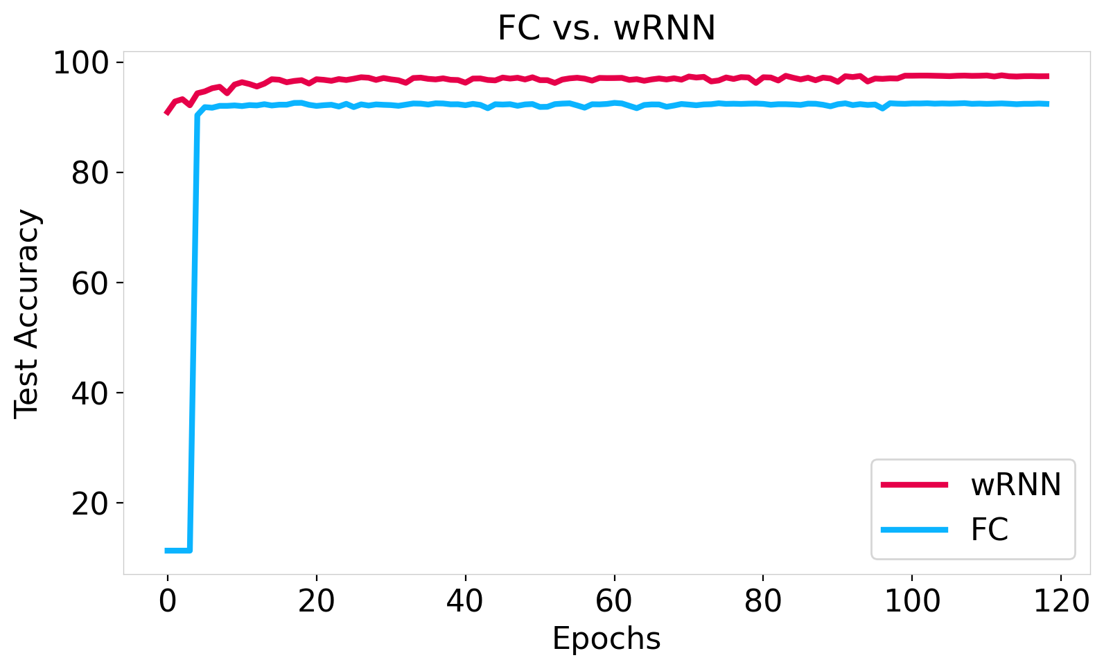
Figure 10: Training curves for a fully connected layer trained on flattened MNIST images (FC) versus the standard wRNN presented in the main text. We see the wRNN still performs significantly better, however the FC model does mimic the rapid learning capability of the wRNN, suggesting that the wRNN’s learning speed may be partially attributable to the wave-field’s memory-tape-like quality.

Additional Ablation: Frozen Encoder & Recurrent Weights.

To further investigate the difference between the wRNN model and a model which simply copies input to a register, we propose to study the relative importance of the encoder weights $\mathbf{V}$ and recurrent connections $\mathbf{U}$ for the wRNN. We hypothesized that the wRNN may preserve greater information in its hidden state by default, and thus may not need to learn a flexible encoding, or perform recurrent processing. To test this, we froze the encoder and recurrent connections, leaving only the decoder (from hidden state to class label) to be trained. In Figure 11 we plot the training curves for a wRNN and iRNN with frozen $\mathbf{U}$ and $\mathbf{V}$. We see that the wRNN performs remarkably better then the iRNN in this setting (89.0% vs. 44.3%), indicating that the wave dynamics do indeed preserve input information by default far better than standard (identity) recurrent connections.

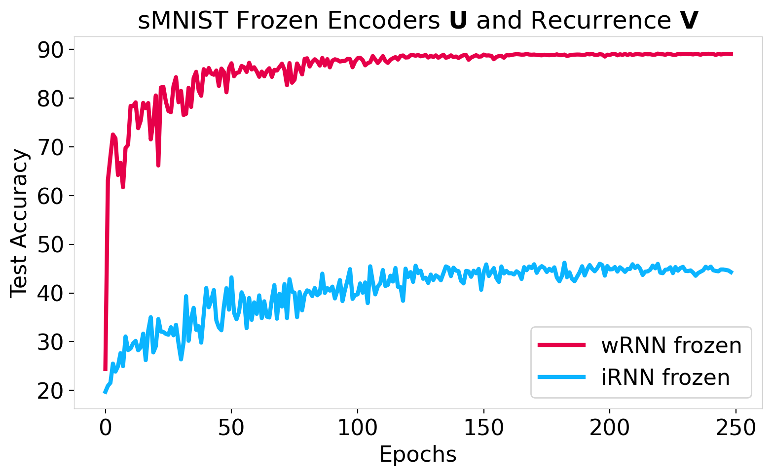
Figure 11: Training curves for wRNN and iRNN models with frozen encoder and recurrent connections ($\mathbf{U}$ & $\mathbf{V}$) on the sMNIST task. We see that the wRNN performs drastically better, indicating that the wRNN requires significantly less flexibility in its encoder and recurrent connections in order to achieve high accuracy.

Additional Ablation: Locally Connected RNN.

In order to test if the emergence and maintenance of waves requires the weight sharing of the convolution operation, or is simply due to local connectivity, we perform an additional experiment where we use the exact same model as the default wRNN, however we remove weight sharing across locations of the hidden state. This amounts to replacing the convolutional layer with an untied ‘locally connected’ layer. In practice, when initialized with same the shift-initialization we find that such a model does indeed exhibit traveling waves in its hidden state as depicted in Figure 12. Although we notice that the locally connected network does train to comparable accuracy with the convoluitional wRNN on sMNIST, we present this preliminary result as a simple ablation study and leave further tuning of the performance of this model on sequence tasks for future work.

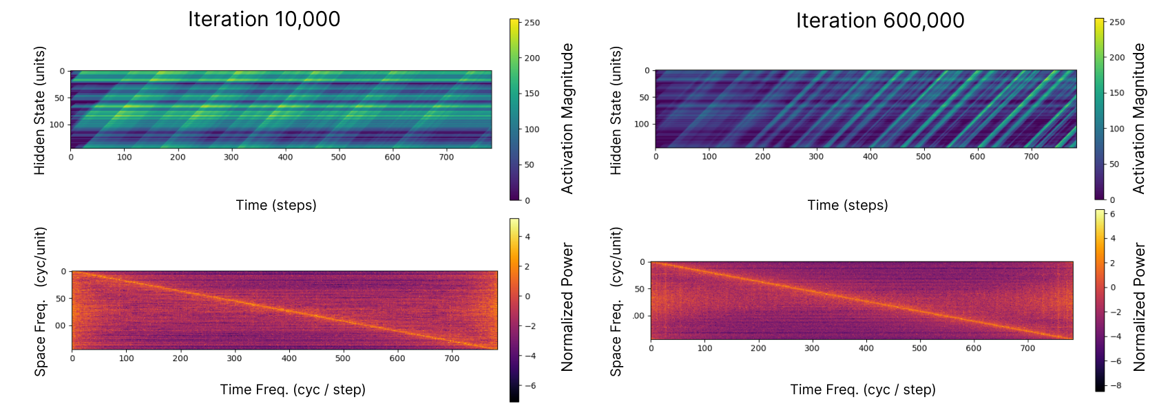
Figure 12: Hidden state and 2D Fourier transform for a locally connected RNN showing the existence of traveling waves. These results imply that it is simply local connectivity which is important for the emergence of traveling waves rather than shared weights.

Additional Visualizations of Copy Task.

Here we include additional visualizations of the larger iRNN (n=625) for the copy task. We see that while it performs slightly better than the smaller iRNN (n=100) it still performs very poorly in comparison with the wRNN.

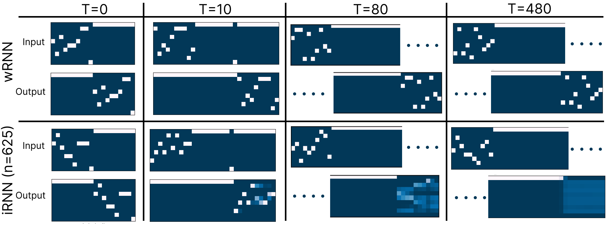
Figure 13: Examples from the copy task for the larger iRNN (n=625) and wRNN (n=100, c=6) as shown in the main text. We see the larger iRNN does slightly better than the small iRNN (n=100) shown in Figure 4, but still significantly worse than the wRNN. These results clearly show that the iRNN does not have the appropriate machinery for storing memories over long sequences while the wRNN does.

On the Emergence of Traveling Waves.

In this section we expand on the results of Figure 9 and include additional results pertaining to the emergence of traveling waves in recurrent neural networks with different connectivity and initialization schemes. Specifically, in Figure 15 we show the hidden state visualization for models with varying initalizations. We see that models with shift-initialization exhibit waves directly from initialization, while randomly initialized convolutional models do not initially exhibit waves but learn to exhibit them during training, and identity initialized models never learn to exhibit waves. Furthermore, in Figure 14 we show the respective training curves for randomly initialized and identity initialized wRNNs. We see that the randomly initialized wRNN achieves higher final accuracy in correspondence with the emergence of traveling waves, reinforcing the conclusion that traveling waves are ultimately beneficial for sequence modeling performance.

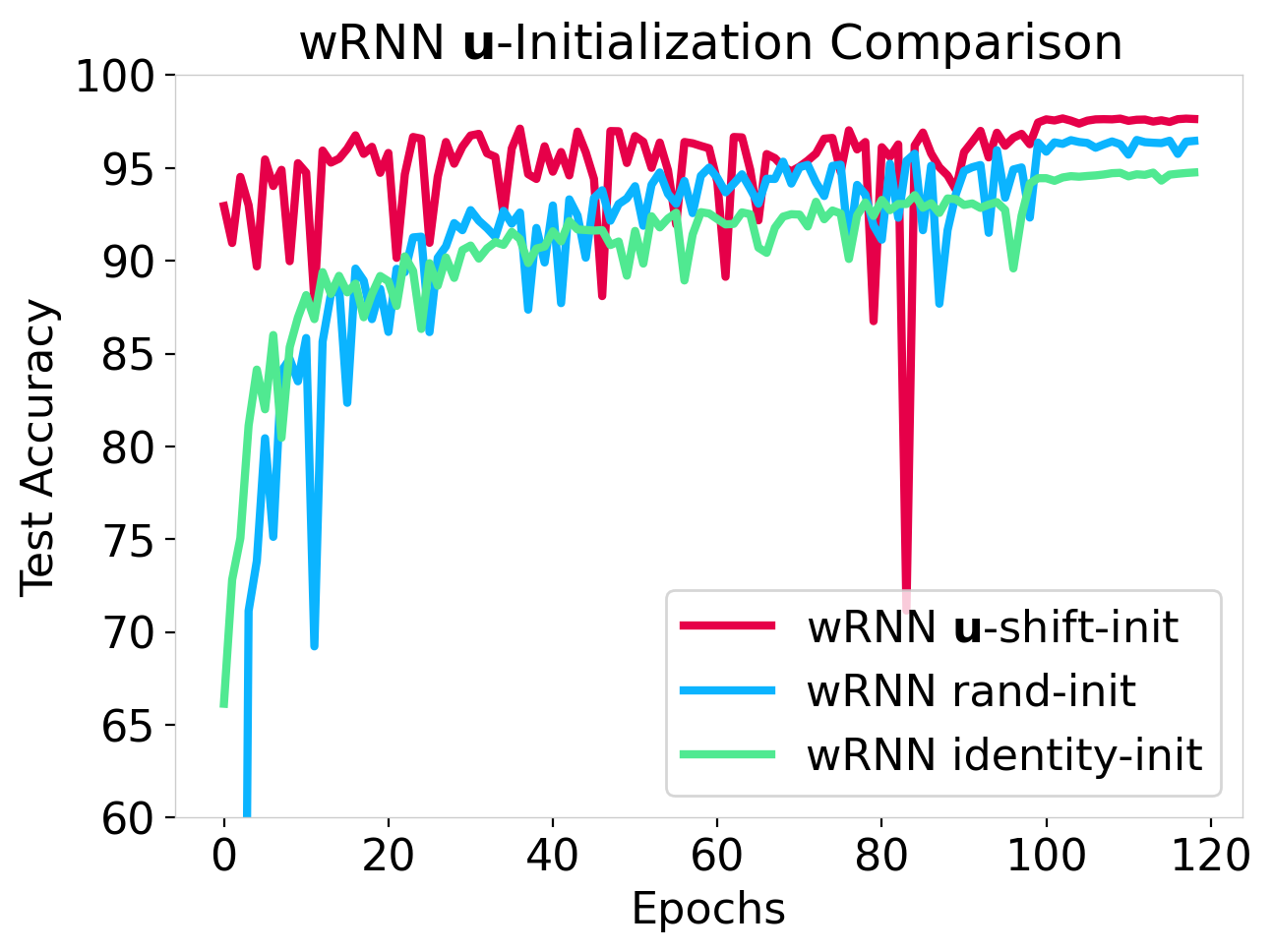
Figure 14: Training curve on the sMNIST task for a wRNN with three different initialization schemes: $\mathbf{u}$-shift (default), random ($\mathcal{U}(-\frac{1}{\sqrt{n}},\frac{1}{\sqrt{n}})$), and identity (dirac). We see that the random initalization does not have the same rapid learning speed as the $\mathbf{u}$-shift initialization, however, it does still achieve significantly higher final accuracy than the identity initialization, implying traveling waves are beneficial to performance.

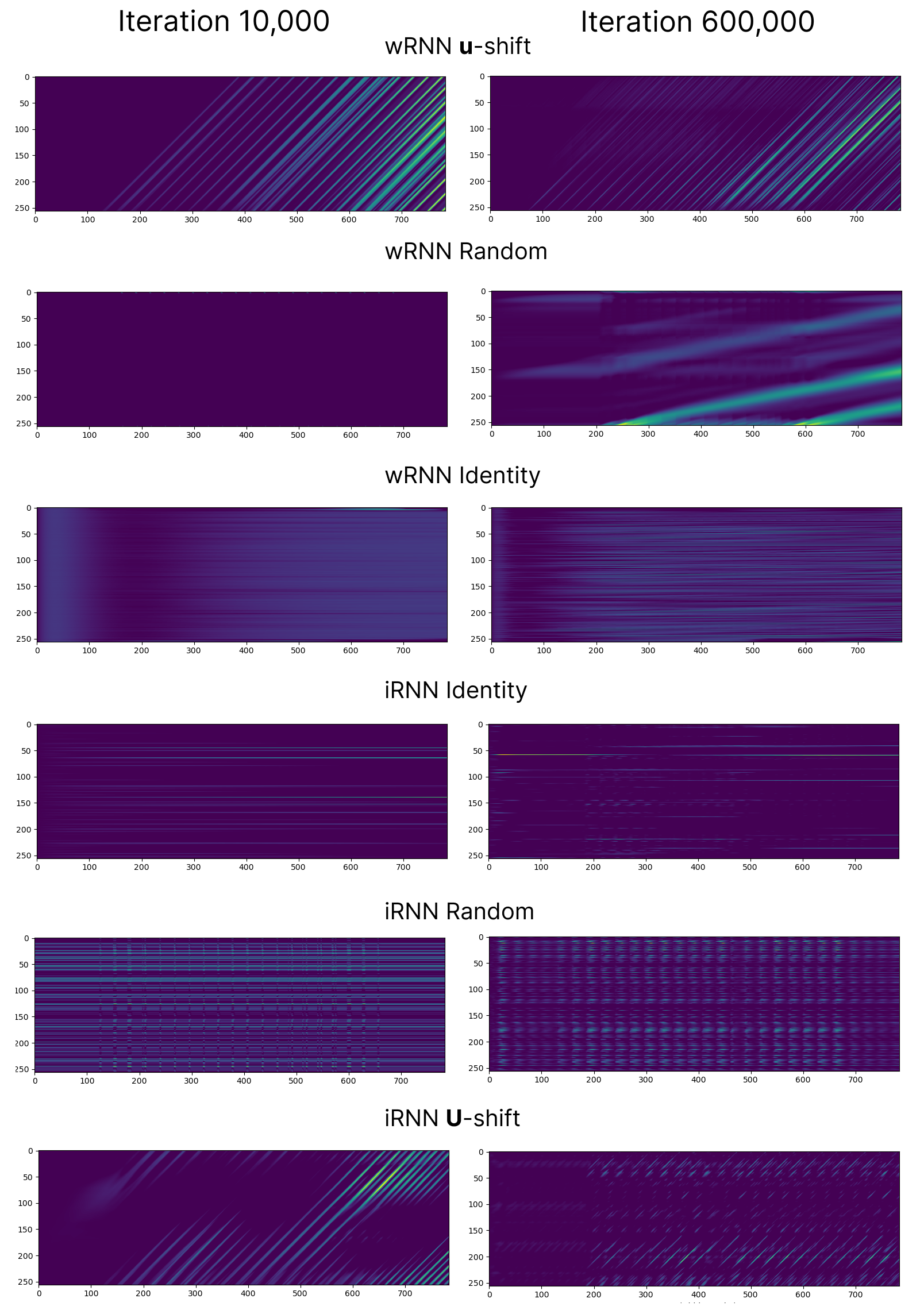
Figure 15: Visualization of hidden state (y-axis is hidden units) over timesteps (x-axis) for a variety of different models and initalizations for $\mathbf{U}$. We see that the wRNN with $\mathbf{u}$-shift initialization achieves the most consistent waves throughout training. Interestingly, some other models learn to achieve traveling waves despite not having them at initalization (wRNN with random (kaming uniform) initialization); while other models, (iRNN with $\mathbf{U}$-shift) initially have stronger traveling waves, and slowly lose them throughout training. We see the wRNN with identity (dirac) initialization never learns waves despite using convolutional recurrent connections.

References

- [1] Martin Arjovsky, Amar Shah, and Yoshua Bengio. Unitary evolution recurrent neural networks. In Proceedings of the 33rd International Conference on International Conference on Machine Learning - Volume 48, ICML’16, page 1120–1128. JMLR.org, 2016.
- [2] Jimmy Ba, Geoffrey Hinton, Volodymyr Mnih, Joel Z. Leibo, and Catalin Ionescu. Using fast weights to attend to the recent past, 2016.
- [3] Gabriel Benigno, Roberto Budzinski, Zachary Davis, John Reynolds, and Lyle Muller. Waves traveling over a map of visual space can ignite short-term predictions of sensory input. Research Square Platform LLC, August 2022.
- [4] Charles F. Cadieu, Ha Hong, Daniel L. K. Yamins, Nicolas Pinto, Diego Ardila, Ethan A. Solomon, Najib J. Majaj, and James J. DiCarlo. Deep neural networks rival the representation of primate it cortex for core visual object recognition. PLOS Computational Biology, 10(12):1–18, 12 2014.
- [5] M. P. Cagigal, L. Vega, and P. Prieto. Movement characterization with the spatiotemporal fourier transform of low-light-level images. Applied Optics, 34(11):1769, April 1995.
- [6] Bo Chang, Minmin Chen, Eldad Haber, and Ed H. Chi. AntisymmetricRNN: A dynamical system view on recurrent neural networks. In International Conference on Learning Representations, 2019.
- [7] Ricky T. Q. Chen, Yulia Rubanova, Jesse Bettencourt, and David K Duvenaud. Neural ordinary differential equations. In S. Bengio, H. Wallach, H. Larochelle, K. Grauman, N. Cesa-Bianchi, and R. Garnett, editors, Advances in Neural Information Processing Systems, volume 31. Curran Associates, Inc., 2018.
- [8] Yusi Chen, Huanqiu Zhang, and Terrence J. Sejnowski. Hippocampus as a generative circuit for predictive coding of future sequences. bioRxiv, 2022.
- [9] Narsimha Reddy Chilkuri and Chris Eliasmith. Parallelizing legendre memory unit training. In Marina Meila and Tong Zhang, editors, Proceedings of the 38th International Conference on Machine Learning, volume 139 of Proceedings of Machine Learning Research, pages 1898–1907. PMLR, 18–24 Jul 2021.
- [10] Zachary W. Davis, Gabriel B. Benigno, Charlee Fletterman, Theo Desbordes, Christopher Steward, Terrence J. Sejnowski, John H. Reynolds, and Lyle Muller. Spontaneous traveling waves naturally emerge from horizontal fiber time delays and travel through locally asynchronous-irregular states. Nature Communications, 12(1), October 2021.
- [11] Zachary W. Davis, Lyle Muller, Julio Martinez-Trujillo, Terrence Sejnowski, and John H. Reynolds. Spontaneous travelling cortical waves gate perception in behaving primates. Nature, 587(7834):432–436, October 2020.
- [12] Jeffrey L. Elman. Finding structure in time. Cognitive Science, 14(2):179–211, 1990.
- [13] N. Benjamin Erichson, Omri Azencot, Alejandro Queiruga, Liam Hodgkinson, and Michael W. Mahoney. Lipschitz recurrent neural networks. In International Conference on Learning Representations, 2021.
- [14] G Bard Ermentrout and David Kleinfeld. Traveling electrical waves in cortex: insights from phase dynamics and speculation on a computational role. Neuron, 29(1):33–44, 2001.
- [15] Alex Graves, Greg Wayne, and Ivo Danihelka. Neural turing machines, 2014.
- [16] Alex Graves, Greg Wayne, Malcolm Reynolds, Tim Harley, Ivo Danihelka, Agnieszka Grabska-Barwińska, Sergio Gómez Colmenarejo, Edward Grefenstette, Tiago Ramalho, John Agapiou, Adrià Puigdomènech Badia, Karl Moritz Hermann, Yori Zwols, Georg Ostrovski, Adam Cain, Helen King, Christopher Summerfield, Phil Blunsom, Koray Kavukcuoglu, and Demis Hassabis. Hybrid computing using a neural network with dynamic external memory. Nature, 538(7626):471–476, October 2016.
- [17] Albert Gu, Karan Goel, and Christopher Re. Efficiently modeling long sequences with structured state spaces. In International Conference on Learning Representations, 2022.
- [18] Albert Gu, Caglar Gulcehre, Tom Le Paine, Matt Hoffman, and Razvan Pascanu. Improving the gating mechanism of recurrent neural networks, 2020.
- [19] K. He, X. Zhang, S. Ren, and J. Sun. Delving deep into rectifiers: Surpassing human-level performance on imagenet classification. In 2015 IEEE International Conference on Computer Vision (ICCV), pages 1026–1034, Los Alamitos, CA, USA, dec 2015. IEEE Computer Society.
- [20] Mikael Henaff, Arthur Szlam, and Yann LeCun. Recurrent orthogonal networks and long-memory tasks. In Maria Florina Balcan and Kilian Q. Weinberger, editors, Proceedings of The 33rd International Conference on Machine Learning, volume 48 of Proceedings of Machine Learning Research, pages 2034–2042, New York, New York, USA, 20–22 Jun 2016. PMLR.
- [21] Sepp Hochreiter and Jürgen Schmidhuber. Long short-term memory. Neural computation, 9(8):1735–1780, 1997.
- [22] Anil Kag, Ziming Zhang, and Venkatesh Saligrama. Rnns incrementally evolving on an equilibrium manifold: A panacea for vanishing and exploding gradients? In International Conference on Learning Representations, 2020.
- [23] T. Anderson Keller and Max Welling. Topographic vaes learn equivariant capsules. In Advances in Neural Information Processing Systems, volume 34, pages 28585–28597. Curran Associates, Inc., 2021.
- [24] T. Anderson Keller and Max Welling. Neural wave machines: Learning spatiotemporally structured representations with locally coupled oscillatory recurrent neural networks. In Proceedings of the 40th International Conference on Machine Learning, Proceedings of Machine Learning Research. PMLR, 2023.
- [25] Jonas Kubilius, Martin Schrimpf, Ha Hong, Najib J. Majaj, Rishi Rajalingham, Elias B. Issa, Kohitij Kar, Pouya Bashivan, Jonathan Prescott-Roy, Kailyn Schmidt, Aran Nayebi, Daniel Bear, Daniel L. K. Yamins, and James J. DiCarlo. Brain-Like Object Recognition with High-Performing Shallow Recurrent ANNs. In H. Wallach, H. Larochelle, A. Beygelzimer, F. D’Alché-Buc, E. Fox, and R. Garnett, editors, Neural Information Processing Systems (NeurIPS), pages 12785—-12796. Curran Associates, Inc., 2019.
- [26] Quoc V. Le, Navdeep Jaitly, and Geoffrey E. Hinton. A simple way to initialize recurrent networks of rectified linear units, 2015.
- [27] Hyodong Lee, Eshed Margalit, Kamila M. Jozwik, Michael A. Cohen, Nancy Kanwisher, Daniel L. K. Yamins, and James J. DiCarlo. Topographic deep artificial neural networks reproduce the hallmarks of the primate inferior temporal cortex face processing network. bioRxiv, 2020.
- [28] Mario Lezcano-Casado and David Martínez-Rubio. Cheap orthogonal constraints in neural networks: A simple parametrization of the orthogonal and unitary group, 2019.
- [29] S. Li, W. Li, C. Cook, C. Zhu, and Y. Gao. Independently recurrent neural network (indrnn): Building a longer and deeper rnn. In 2018 IEEE/CVF Conference on Computer Vision and Pattern Recognition (CVPR), pages 5457–5466, Los Alamitos, CA, USA, jun 2018. IEEE Computer Society.
- [30] Lyle Muller, Frédéric Chavane, John Reynolds, and Terrence J. Sejnowski. Cortical travelling waves: mechanisms and computational principles. Nature Reviews Neuroscience, 19(5):255–268, March 2018.
- [31] Lyle Muller, Giovanni Piantoni, Dominik Koller, Sydney S Cash, Eric Halgren, and Terrence J Sejnowski. Rotating waves during human sleep spindles organize global patterns of activity that repeat precisely through the night. eLife, 5, November 2016.
- [32] Antonio Orvieto, Samuel L Smith, Albert Gu, Anushan Fernando, Caglar Gulcehre, Razvan Pascanu, and Soham De. Resurrecting recurrent neural networks for long sequences, 2023.
- [33] Adam Paszke, Sam Gross, Francisco Massa, Adam Lerer, James Bradbury, Gregory Chanan, Trevor Killeen, Zeming Lin, Natalia Gimelshein, Luca Antiga, Alban Desmaison, Andreas Kopf, Edward Yang, Zachary DeVito, Martin Raison, Alykhan Tejani, Sasank Chilamkurthy, Benoit Steiner, Lu Fang, Junjie Bai, and Soumith Chintala. Pytorch: An imperative style, high-performance deep learning library. In Advances in Neural Information Processing Systems 32, pages 8024–8035. 2019.
- [34] Stéphane Perrard, Emmanuel Fort, and Yves Couder. Wave-based turing machine: Time reversal and information erasing. Physical review letters, 117(9):094502, 2016.
- [35] David W. Romero, Robert-Jan Bruintjes, Jakub Mikolaj Tomczak, Erik J Bekkers, Mark Hoogendoorn, and Jan van Gemert. Flexconv: Continuous kernel convolutions with differentiable kernel sizes. In International Conference on Learning Representations, 2022.
- [36] T. Konstantin Rusch and Siddhartha Mishra. Coupled oscillatory recurrent neural network (cornn): An accurate and (gradient) stable architecture for learning long time dependencies. In International Conference on Learning Representations, 2021.
- [37] T. Konstantin Rusch and Siddhartha Mishra. Unicornn: A recurrent model for learning very long time dependencies, 2021.
- [38] T Konstantin Rusch, Siddhartha Mishra, N Benjamin Erichson, and Michael W Mahoney. Long expressive memory for sequence modeling. In International Conference on Learning Representations, 2022.
- [39] Adam Santoro, Sergey Bartunov, Matthew Botvinick, Daan Wierstra, and Timothy Lillicrap. One-shot learning with memory-augmented neural networks, 2016.
- [40] Xingjian Shi, Zhourong Chen, Hao Wang, Dit-Yan Yeung, Wai kin Wong, and Wang chun Woo. Convolutional lstm network: A machine learning approach for precipitation nowcasting, 2015.
- [41] Corentin Tallec and Yann Ollivier. Can recurrent neural networks warp time?, 2018.
- [42] James C.R. Whittington, Timothy H. Muller, Shirley Mark, Guifen Chen, Caswell Barry, Neil Burgess, and Timothy E.J. Behrens. The tolman-eichenbaum machine: Unifying space and relational memory through generalization in the hippocampal formation. Cell, 183(5):1249–1263.e23, 2020.
- [43] Łukasz Kaiser and Ilya Sutskever. Neural gpus learn algorithms, 2016.