A joint modeling approach to study the association between subject-level longitudinal marker variabilities and repeated outcomes

Abstract

Women are at increased risk of bone loss during the menopausal transition; in fact, nearly 50% of women’s lifetime bone loss occurs during this time. The longitudinal relationships between estradiol (E2) and follicle-stimulating hormone (FSH), two hormones that change have characteristic changes during the menopausal transition, and bone health outcomes are complex. However, in addition to level and rate of change in E2 and FSH, variability in these hormones across the menopausal transition may be an important predictor of bone health, but this question has yet to be well explored. We introduce a joint model that characterizes individual mean estradiol (E2) trajectories and the individual residual variances and links these variances to bone health trajectories. In our application, we found that higher FSH variability was associated with declines in bone mineral density (BMD) before menopause, but this association was moderated over time after the menopausal transition. Additionally, higher mean E2, but not E2 variability, was associated with slower decreases in during the menopausal transition. We also include a simulation study that shows that naive two-stage methods often fail to propagate uncertainty in the individual-level variance estimates, resulting in estimation bias and invalid interval coverage.

Bone mineral density, Estradiol, Follicle-stimulating hormone, Joint models; Subject-level variability; Variance component priors

1 Introduction

Osteoporosis, or low levels of bone mineral density (BMD), is a major public health issue as it increases the risk for fracture, a major cause of hospitalizations and morbidity (Marshall and others, 1996). Although osteoporosis prevalence increases with age (Alswat, 2017), the loss of bone mass begins during midlife (age 40-64 years) (Hunter and Sambrook, 2000). For women, declines in BMD accelerate during the menopausal transition (Riggs and Melton, 1992; Ji and Yu, 2015), a period of rapid endocrinologic and physiologic time surrounding the final menstrual period (FMP). While population level patterns of mean level and change in BMD during the midlife and late adulthood are well-established, it is equally vital to model and predict individual trajectories of bone parameters to support advances in precision medicine and tailored individualized treatments.

For midlife women, BMD tends to decline gradually until approximately one to two years prior to the FMP, where there is an acceleration in the decline in BMD (Sowers and others, 2000; Greendale and others, 2019). (Sirola and others, 2003; Recker and others, 2000; Finkelstein and others, 2008). This rate of this decline then decelerates approximately two years after the FMP, but the decline continues throughout the post-menopause (Sowers and others, 2000; Greendale and others, 2019; Sirola and others, 2003; Recker and others, 2000; Finkelstein and others, 2008). Previous studies have examined associations between estradiol (E2) and BMD during the menopausal transition.These studies have established a general positive association between mean E2 levels and BMD (Sowers and others, 2000; Ebeling and others, 1996; Park and others, 2021). However, most of these studies have either been cross-sectional or over a relatively short time period, thereby limiting the ability to examine individual-level changes in E2. Importantly, these studies have focused on mean associations between hormones and bone outcomes, mostly at the population level. The association between individual E2 trajectories, and in particular, individual level E2 variability and BMD changes in peri-and post-menopausal women over a longer time period has not yet been studied.

In addition to E2, there are characteristic changes in follicle-stimulating hormone (FSH) during the menopausal transition, with increases beginning approximately five years before the FMP (Randolph and others, 2011). In the literature, there is an ongoing discourse as to which sex hormone – E2 or FSH – drives changes in bone across the menopausal transition. Chin (2018) examined the longitudinal relationship between FSH and BMD in peri-menopausal women and revealed that “rate of bone loss was inversely associated with FSH level in all subjects, regardless of BMD value”. However, Gourlay and others (2011) did not find a statistically significant relationship between high baseline FSH and decreases in BMD in postmenopausal younger women. These findings suggest that FSH levels may have the strongest association with bone loss during the midlife before the menopausal transition. Like the literature on E2, the FSH literature has largely been focused on a population health approach, utilizing mean levels of FSH as predictors. However, both E2 and FSH can fluctuate substantially within individual women and this fluctuation has been shown to be significantly associated with various health outcomes (Harlow and others, 2000; Uhler and others, 2005). It would thus be of interest to understand how intra-individual variabilities, as well as overall mean hormone levels, affect women’s bone health outcomes.

1.1 Study of Women’s Health Across the Nation Dataset

Study Population

The Study of Women’s Health Across the Nation (SWAN) is an ongoing multi-site longitudinal cohort study of the menopausal transition and aging. At study baseline in 1996, study participants were age 42-52 years, with an intact uterus and at least one ovary, had menses in the previous 3 months and were free of exogenous hormone use in the previous 3 months. By design, SWAN includes a sample that is racially/ethnically diverse, including white, Black, Hispanic, Chinese, and Japanese women. Since it began in 1996, there have been 17 near-annual study visits. For detailed descriptions of the measurement timings and cohort characteristics, we refer the reader to Sowers and others (2000).

At baseline, the original SWAN cohort included 3,302 women. Only five of the seven clinical sites participated in the bone protocol; thus the SWAN Bone Cohort included 2,365 women. The analytic sample included SWAN Bone Cohort women with observed sex hormone, observed FMP, and observed DEXA data across a minimum of 2 visits; 912 women were excluded for either having missing hormone values, unobserved (missing) FMP, or only baseline visits. Additional exclusion criteria included women who took hormone therapy (HRT) during their visits (n=479), since these medications can suppress BMD decline even after stopping HRT (Gambacciani and Levancini, 2014). The final analytic dataset comprised 974 women with 9,858 measurements.

Measures

Estradiol (pg/mL) and FSH (mIU/m) measurements were assayed from serum collected at baseline and during annual follow-up visits. At all visits, blood was collected fasted and during the follicular phase of the menstrual cycle (days 2-5). Details of the blood collection protocol and laboratory methodology for E2 and FSH have been published (Randolph 2011). At each study visit, participants underwent a DEXA scan with a Hologic densitomte (Hologic, Inc., Waltham, Massachusetts) to assess BMD of the femoral neck. Across the clinical sites, a calibration protocol for the densitometers was established and ongoing quality control measures were undertaken Greendale and others (2019). Covariates included body mass index (BMI) and chronological age. BMI was calculated as measured weight (in kilograms) divided by measured height (in meters) squared. Chronological age was calculated as date of visit minus date of birth.

Variable	Statistic	Value	n
Longitudinal Predictor	Mean/SD
E2 Residuals		-0.01 (1.15)	9,858
FSH Residuals		0.02 (0.90)	9,858
Health Outcome	Mean/SD
BMD Residuals		0.00 (0.23)	9,858
Adjusted Covariates	Mean/SD
Baseline BMI		27.28 (6.83)	9,858
Baseline Age		46.29 (2.60)	9,858

Table 1: Descriptive statistics of the dataset, based on 974 individuals in the Study of Women’s Health Across the Nation.

All participants provided written informed consent at each study visit and the protocols at each site were approved by each site’s Institutional Review Board.

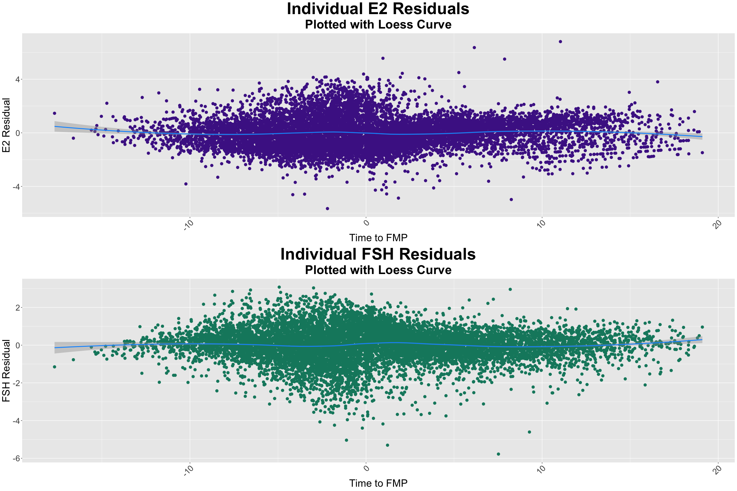
Figure 1: Plot of E2 observations (top figure) and FSH observations (bottom figure) for all individuals in our dataset, plotted over time to FMP. A loess curve has been added to each plot to show the average population trend. Both E2 and FSH observations (before detrending) had been $\log_{2}$ transformed.

Statistical Analysis

Based upon population-level data, E2 and FSH demonstrate well-established and characteristic changes during the menopausal transition (Randolph and others, 2004). To remove the population trend in the hormones, we fit a loess curve to each hormone using the loess function in R and subtracted each women’s measurements from this loess fit. We performed all of the following analyses in Section 4 using these hormone residuals. Figure 1 displays the E2 residuals and the FSH residuals. We also lagged these residuals by 1 visit, for ease of interpretation.

For all analyses, the time scale was considered as time to/from the FMP. FMP was defined retrospectively following 12 months of amenorrhea. Longitudinal analyses were conducted to estimate the association between hormone variability and femoral neck BMD . Additionally, interaction terms were included and examined to determine whether the relationships change over time. Thus, our statistical objective is to develop a modeling framework that can estimate the individual level mean and variance of a longitudinal marker, and also link these estimates to the longitudinal outcome of interest via a regression function.

A base 2 log transformation was used on the outcome of interest (BMD). In order to focus on the individual level changes in BMD trajectories, measurements were detrended by fitting a loess curve to all measurements (using the loess function in R) and then subtracting the individual measurements from the fitted loess values. Figure 2 displays the residual BMD values after our detrending, in order to simplify subject level trends as lower-level polynomial functions; in practice a linear approximation appeared sufficient after population-level detrending.

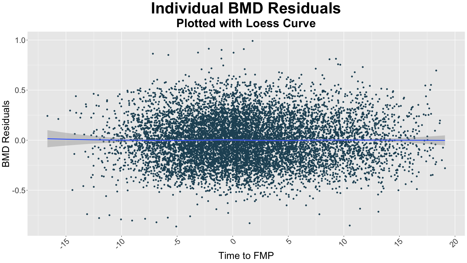
Figure 2: Plot of BMD residuals for all individuals in our dataset, plotted over time to FMP. A loess curve has been added to show the average population trend of the residuals. Prior to detrending, the BMD observations had been $\log_{2}$ transformed.

Finally, the outcome model was adjusted for baseline BMI and baseline age. To ease interpretability, baseline BMI measurements were standardized to be relative to the population mean (baseline) BMI and baseline age was centered relative to the population mean (baseline) age. Summary statistics of all variables in the joint model are shown in Table 1.

1.2 Statistical Models for Longitudinal Outcomes

Models with longitudinal outcomes allow researchers to understand relationships between variables across time, and potentially how these associations change across time. These methods tend to fall into two broad classes: generalized estimating equations (Liang and Zeger, 1986) methods and mixed-effects models or structural equation modeling (SEM)-type growth curve models. While the GEE approach has several advantages, such as robustness in the case of misspecified marginal correlations, it is not designed for studying individual-level random effects. In our particular setting, we are primarily interested in relating the individual-level means and variances to the health outcome, and so our modeling approach needs to explicitly estimate the individual random effects. Mixed-effects models have been studied extensively (Laird and Ware, 1982; Greene, 2005; Diggle and others, 2013) and are well-suited for estimating multilevel or hierarchical data. These models can also easily handle interactions with time, which can be specified as an additional covariate. A drawback of the mixed effects model is that the predictor variable is treated as fixed data, rather than being estimated as part of the model. Latent growth curve (LGC) models on the other hand provide a framework for estimating two or more trajectories simultaneously. In the latent growth curve specification, the random effects are modeled as latent variables, which can be shown to be mathematically equivalent to the random effects specification in mixed effects models (Zhang and others, 2022). Generally, LGC models are not well-suited for datasets with moderate to large number of observations per individuals, since the LGC framework requires each visit or timepoint to be a unique predictor. Mixed-effects models, on the other hand, allow the time variable to be univariate and can more easily handle many observations per individual (McNeish and Matta, 2018).

One noticeable gap in both frameworks is that the individual residual variances in the predictors are usually treated as nuisance parameters, rather than as potentially important entities for predicting the outcome. There has been a growing collection of research (Elliott and others, 2012; Jiang and others, 2015; Gao and others, 2022) on joint models that evaluate the associations between within subject variability and outcomes of interest; however, these models have focused on cross-sectional outcomes. Methods for estimating individual variances from longitudinal markers to predict longitudinal outcomes are currently lacking in the literature. Our proposed model contributes to this research by providing a general method for estimating individual-level variability from a longitudinal marker and using this variability to predict a longitudinal time-varying outcome. Our specification can easily extend to incorporating a time-varying variance parameterization, as demonstrated by simulation studies.

The rest of this paper is organized as follows. We describe our Bayesian joint model framework in Section 2. Section 3 introduces simulation studies that demonstrate that our model produces less biased estimates of the outcome regression coefficients than alternative two-stage models that do not account for the statistical uncertainty in the individual means and variances. We apply our model in Section 4 to the SWAN dataset, where we focus on the study of the associations between E2 and FSH mean trajectories and variances and BMD outcomes in midlife women. To the best of our knowledge, this is the first scientific assessment of using individual level variances of E2 and FSH to predict declines in longitudinal bone measures. Finally, in Section 5, we discuss the implications of our findings along with future directions. Our supplementary material contains further details about the model validation for the data analysis (e.g. posterior predictive checks). R code to run our model can be found at the following GitHub repository: https://github.com/realirena/jelo/.

2 Joint Model

In this section, we describe our proposed model, which specifies our longitudinal predictor $X_{ij}$, which is measured at each timepoint $t_{ij},j=1,\ldots,n_{i}$, for each subject $i=1,\ldots,N$ where $n_{i}$ is the total number of observations for individual $i$. Our model links the individual-specific vectors of regression coefficients and residual variance estimates of $X_{ij}$ to the longitudinal outcome $Y_{ij}$.

2.1 Likelihood

2.1.1 Longitudinal Marker Model

The model for the longitudinal predictor is given by:

$$X_{ij}\mid\mathbf{b}_{i},s_{i}\sim\mathcal{N}\left(\mu(t_{ij};\mathbf{b}_{i}),s_{i}^{2}\right),$$ (1)

$$j=1,\ldots,n_{i},{\sf~{}independently~{}for~{}}i=1,\ldots,N,$$

$$\bm{b}_{i}\overset{\sf indep.}{\sim}\mathcal{N}_{P}(\boldsymbol{\alpha},\Sigma),{\sf~{}independently~{}for~{}}i=1,\ldots,N,$$ (2)

where $\mathcal{N}(\mu,s)$ represents a Gaussian distribution with mean $\mu$ and variance parameter $s$ and $\mathcal{N}_{P}(\boldsymbol{\alpha},\Sigma)$ is the $P$-dimensional generalization the Gaussian distribution with mean vector $\boldsymbol{\alpha}$ and variance-covariance matrix $\Sigma$. $\mu(t;\mathbf{b}_{i})$ is function of time and a vector of $P$ regression coefficients, $\bm{b}_{i}=(b_{i1},\ldots,b_{iP})^{{\sf T}}$. $\boldsymbol{\alpha}=(\alpha_{1},\ldots,\alpha_{P})^{{\sf T}}$ is a vector of population mean regression coefficients.

Priors for $\boldsymbol{\alpha}$:

We assume that $\boldsymbol{\alpha}=(\alpha_{1},\ldots,\alpha_{P})^{\sf T}$, are drawn from a $P$ dimensional Normal distribution:

$$\boldsymbol{\alpha}~{}{\sim}~{}\mathcal{N}_{P}(0,\xi_{0}^{2}I_{P\times P}),$$ (3)

$$\Sigma=KLK,~{}K={\rm diag}\{k_{1},\ldots,k_{P}\},$$ (4)

$$k_{p}\sim\textsf{half-Cauchy}(0,\tau_{0}),p=1,\ldots,P,L\sim{\sf LKJ}(\zeta),$$ (5)

where $K={\rm diag}\{k_{1},\ldots,k_{P}\}$ is a diagonal matrix and $L$ is a correlation matrix, with a Lewandowski-Kurowicka-Joe (LKJ) diffuse prior (Lewandowski and others, 2009). As in the case of the hyperpriors for the individual variance parameters, the values of $\xi_{0},\tau_{0},\zeta$ parameters are set a priori, here as $\xi=1,\tau_{0}=2.5,\zeta=1$.

Prior for $s_{i}^{2}$

We assume that the individual residual variances, $s_{i}^{2}$’s are drawn from a log-Normal distribution, i.e.:

$$\log(s_{i}^{2})\sim\mathcal{N}(\nu,\psi^{2}),$$ (6)

$$\nu\sim\mathcal{N}(m,\xi^{2}),\psi\sim\textsf{half-Cauchy}(0,\tau),$$ (7)

where the values of hyperprior parameters $m,\xi,\tau$ are set a priori. In our application, we set $m=0$, $\xi=10$, $\tau=2.5$, so that the priors are weakly informative. Following the recommendations made in Gelman (2006), we use the half-Cauchy hyperprior on $\psi$, the square root of the variance parameter. Although the inverse-Gamma distribution is the conjugate prior for the variance parameter of a Gaussian distribution, inferences using the inverse-Gamma distribution can be extremely sensitive to the choice of hyperparameter values (Gelman, 2006, p. 524). The half-Cauchy distribution avoids this potential issue due to its heavier tail, which still allows for higher variance values.

Time-varying variance:

A model that would allow the individual variances, in addition to the means, to change over time could have the following parameterization:

$$\log(s_{ij}^{2})=g(t_{ij};\boldsymbol{\lambda}_{i}),$$ (8)

$$\boldsymbol{\lambda}_{i}\sim\mathcal{N}(\boldsymbol{\delta},\boldsymbol{\Psi}),$$ (9)

where $\boldsymbol{\lambda}_{i}$ is a $P_{S}$ dimensional vector that represents the individual-level variance regression coefficients, with $P_{S}$ being specified in advanced. $\boldsymbol{\delta},\boldsymbol{\Psi}$ can be estimated with the same priors specified in Equation 5. Simulation study 3.2 evaluates the relative advantages of this time-varying variance over the time-invariant one under different data generating scenarios. In practice when applying our model to the SWAN dataset, we found that the time-varying variance model had severe convergence issues compared to the time-invariant variance model. We discuss this further in Section 4.

2.1.2 Longitudinal Outcome Model

The outcome variable, $Y_{ij}$, is related to individual-specific mean and variance parameters $\mathbf{b}_{i}$ and $s_{i}$ (Equation 1) via the following specification:

$$Y_{ij}\mid\mathbf{b}_{i},\bm{a}_{i},t_{ij},s_{i}^{2},\mathbf{W}_{i}\sim \mathcal{N}\left(\eta_{ij}(\mu_{ij},t_{ij},s_{i}^{2},\mathbf{W}_{i}),\sigma^{2}\right),$$ (10)

$$i=1,\ldots,N,j=1,\ldots,n_{i},$$

where $\mu_{ij}$ is the mean from the marker model.

This specification allows us to evaluate the direct relationship between the estimate $\mu_{ij}$ and the outcome $Y_{ij}$, rather than linking $X_{ij}$ and $Y_{ij}$ via the mean coefficients $\mathbf{b}_{i}$. This ease of interpretation may be preferred in scientific applications. This also avoids contamination from the time-invariant $\bm{b}_{i}$. The individual residual marker variances, $s_{i}^{2}$, could also be specified similarly if we allow these to vary over time (see simulation study 3.2).

In our application, we focus on simple specifications of $\eta(\cdot)$, e.g., linear models with two-way interactions in order to maintain interpretability of the coefficients. However, extensions with more complex interactions or non-linear mean structures are also possible, with the caveat that the interpretability of the coefficients may be challenging (or near impossible) with higher-order terms.

Priors for $\boldsymbol{\beta}$, $\textbf{a}_{i}$, $\sigma$

For the outcome model, we use independent $\mathcal{N}(0,10^{2})$ priors for each element of the outcome regression parameters ($\boldsymbol{\beta}$, $\boldsymbol{\beta}^{W}$), and a diffuse prior on the outcome residual standard deviation parameter $\sigma\sim\textsf{half-Cauchy}(0,2.5)$, as recommended by Carpenter and others (2017). For $\bm{a}_{i}$, the random effects, we place a multivariate Gaussian prior with mean zero and precision $\tau_{a}$, i.e., $\bm{a}_{i}\sim\mathcal{MVN}(0,\tau_{a})$. In the case of a random intercept $a_{i}$, $\tau_{a}$ can be drawn from a half-Cauchy distribution or, in the case of a vector-valued $\bm{a}_{i}$, $\tau_{a}$ is a covariance matrix, whose values can be drawn from the prior described in Equation 5.

Joint Distribution

Let $D=(Y_{ij},X_{ij},t_{ij},\mathbf{W}_{i})$ denote the observed data, $Z$ = ($\mathbf{b}_{i}$, $s_{i}$, $\bm{a}_{i}$) denote the subject-level latent variables, and $\Theta=(\boldsymbol{\alpha},\Sigma,\xi,\nu_{q},\psi,\boldsymbol{\beta},\boldsymbol{\beta}^{W},\tau_{a},\sigma)$ denote the model parameters. We also let $\pi(\Theta)$ denote the prior distribution of the parameters in $\Theta$:

$$\pi(\Theta)=\pi(\boldsymbol{\alpha})\pi(\Sigma)\pi(\xi)\pi(\nu,\psi)\pi(\boldsymbol{\beta},\boldsymbol{\beta}^{W})\pi(\sigma).$$ (11)

We can then write the joint distribution of $D$, $Z$, and $\Theta$ as

$$P(\Theta,D,Z)\propto \prod^{N}_{i=1}\Big{\{}\frac{1}{\sqrt{(2\pi)|\Sigma|}}{\exp}(-\frac{1}{2}(\mathbf{b}_{i}-\boldsymbol{\alpha})^{{\sf T}}\Sigma^{-1}(\mathbf{b}_{i}-\boldsymbol{\alpha}))$$

$$\times\frac{1}{\sqrt{2\pi\xi^{2}}}{\exp}\left[\frac{(\log(s_{i}^{2})-\nu)^{2}}{2\xi^{2}}\right]$$

$$\times\frac{1}{\sqrt{2\pi|\tau_{a}|}}{\exp}(-\frac{1}{2}\bm{a}_{i}^{{\sf T}}\tau_{a}^{-1}\bm{a}_{i})\Big{\}}$$

$$\times\prod^{N}_{i=1}\prod^{n_{i}}_{j=1}\Big{\{}\frac{1}{\sqrt{2\pi s_{i}^{2}}}{\exp}\left(-\frac{1}{2}\{\dfrac{X_{ij}-\mu_{ij}(t_{ij};\mathbf{b}_{i})}{s_{i}}\}^{2}\right)$$

$$\times\dfrac{1}{\sqrt{2\pi\sigma^{2}}}{\exp}\left(-\frac{1}{2}\frac{(y_{ij}-\eta_{ij}(\mathbf{b}_{i},s_{i},\mathbf{W}_{i},\bm{a}_{i};\boldsymbol{\beta},\boldsymbol{\beta}^{W}))^{2}}{\sigma^{2}}\right)\Big{\}}$$

$$\times\pi(\Theta).$$ (12)

2.2 Posterior Inference

We implemented our joint model using Stan and the rstan package (Stan Development Team, 2020) and obtained posterior estimates via the Hamiltonian Monte Carlo sampler. For our two simulations studies in Sections 3.1 and 3.2 we ran two chains per independent replicate data set, with $2,000$ iterations with $1,000$ burn-in. For the E2 predictor model in Section 4, we ran 2 chains each with 4,000 iterations and 2,000 burn in. For the FSH model, we found that running 2 chains with 2,000 iterations with 1,000 burn in was sufficient for the model to achieve convergence. We conducted visual inspection of the traceplots for all model parameters which indicated non-divergent chains. All of the chains in each model were combined for computing posterior summaries.

We also used Stan’s R-hat convergence diagnostic (Vehtari and others, 2021) to evaluate model convergence. The outcome parameters in both of our models had R-hat values $<$ 1.05. Additionally, model checks of the posterior predictive distribution in the Supplementary Materials indicated that our models generated reasonable predictions for our datasets.

3 Simulation Study

The goal of our simulation studies was to 1) evaluate our model’s operating characteristics and 2) compare against common alternatives that could also be used in modeling individual means and variances as predictors of longitudinal outcomes. For each proposed method and each parameter $\theta$, we assessed the 1) bias (defined as $\dfrac{1}{R}\sum_{r=1}^{R}(\widehat{\theta}^{(r)}-\theta_{0})$ where $\widehat{\theta}^{(r)}$ is the posterior mean of $\theta$ obtained from the $r$-th replication), 2) the coverage rate of the nominal $95\%$ credible intervals (CrI; defined as $\dfrac{1}{R}\sum^{R}_{r=1}\mathbbm{1}\{\theta_{0}\in I_{r}\}$ where $I_{r}$ is the $95\%$ CrI for parameter $\theta$ obtained by computing the 2.5% and 97.5% percentiles of the draws from the posterior distribution for the $r$-th replication, and 3) average length of the 95% CrIs obtained across simulation replicates, defined as $\dfrac{1}{R}\sum^{R}_{r=1}T_{r}$, where $T_{r}$ is the length of $I_{r}$, i.e., the range of the estimated 2.5% and 97.5% posterior quantiles for $\theta$ in replicate $r$.

3.1 Simulation I: Constant Individual Variance Model

For this simulation study, we generated data for N = 300 individuals. We simulate for each individual between 2 to 15 timepoints, which mimics the our application dataset from the SWAN study. Based on these individual timepoints, we simulate the marker values for each individual using the following data generating parameters:

$$X_{ij}\sim\mathcal{N}(\bm{\mu}_{ij},s_{i}^{2}),\bm{\mu}_{ij}=b_{i1}+b_{i2}t_{ij},$$

$$\bm{b}_{i}\sim\mathcal{N}_{2}\left(\boldsymbol{\alpha},\Sigma\right),\boldsymbol{\alpha}=(0,2)^{\sf T},$$

$$\Sigma=\begin{pmatrix}1&-0.05\\ -0.05&1\end{pmatrix},\log(s^{2}_{i})\sim\mathcal{N}(0,0.375^{2}).$$

Figure 3 displays the simulated marker means, marker trajectories, and constant variances that are generated by these specified parameters.

(a)

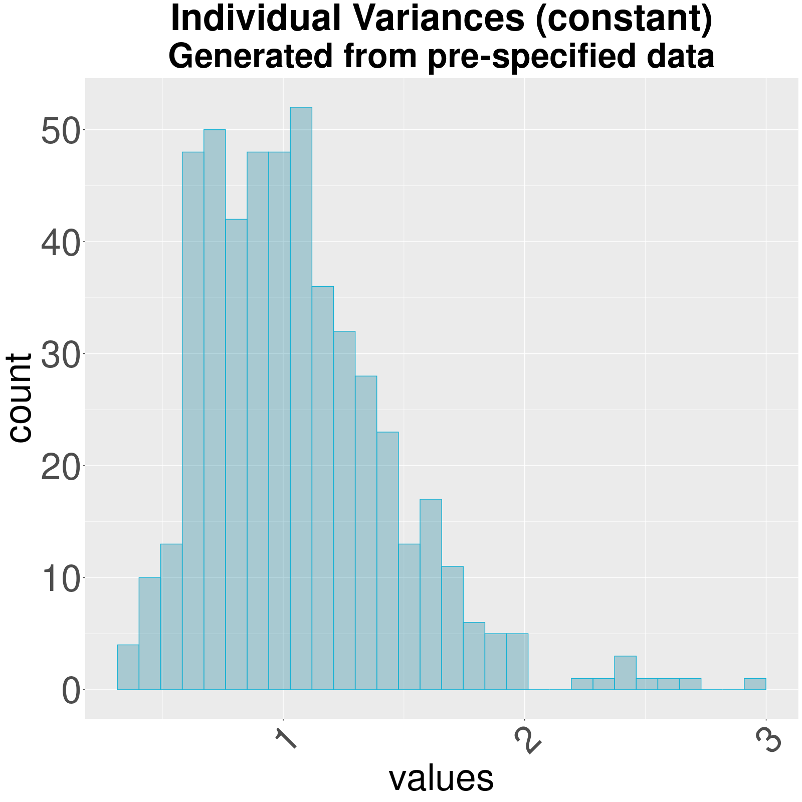
(b)

Figure 3: Histogram of individual variances (left plot) and individual mean and marker trajectories (line plots) for 10 individuals, along with the generated individual variance labelled in each plot.

For the longitudinal outcome, we assumed the following model: $Y_{ij}\sim\mathcal{N}(\eta_{ij}(\mathbf{b}_{i},s_{i},a_{i},t_{ij}),\sigma^{2})$ and set

$$\eta_{ij}(\mathbf{b}_{i},s_{i})=\beta_{0}+\beta_{1}\mu_{ij}+\beta_{2}s_{i}^{2}$$

$$+(\beta_{3}+\beta_{4}\mu_{ij}+\beta_{5}s_{i}^{2})t_{ij}+a_{i},$$

where the true values of $\boldsymbol{\beta}$ are shown in Table 2. We specified the random intercept $a_{i}$ as follows:

$$a_{i}\sim\mathcal{N}(0,0.5^{2}).$$

Lastly, we set $\sigma=0.1$. In this simulation, we did not adjust for other covariates $\mathbf{W}_{i}$ in either submodel. We present the results for 200 replicates in Table 2 for the outcome submodel parameters $\boldsymbol{\beta}$.

3.1.1 Alternative Methods

We compared our approach to two alternative two-stage methods: a two-stage linear mixed model (TSLMM), and a two-stage Bayesian model with longitudinal outcome (TSLO). The TSLO approach is essentially the two-stage version of our joint model, using the posterior mean estimates from the means and variances of the longitudinal marker to predict the outcome in the second stage. We refer to our joint model as the “Jointly Estimated (Model) with Longitudinal Outcome”, or JELO. In the absence of a joint model, these approaches would be reasonable methods for scientific researchers who wish to analyze the associations between a longitudinal predictor and longitudinal outcome. However, as shown in previous literature, two-stage methods often do not correctly preserve the uncertainty associated with estimating the individual random effects from the predictor marker variable (Hickey and others, 2016).

Two-Stage Linear Mixed Models (TSLMM)

In the first stage, we fit a linear mixed model with the nlme package (Pinheiro and others, 2022) with the following specification:

$$X_{ij}=\beta_{0}+b_{i0}+\beta_{1}t_{ij}+b_{i1}t_{ij}+\epsilon_{ij}.$$

We used an unstructured variance-covariance structure for the random effects, which is the default specification for this package.

We obtained the predicted values of $x_{ij}$ using the predict() function. We estimated $s_{i}^{2}$ by first computing the model residuals (e.g. $X_{ij}-(\widehat{B}_{i0}+\widehat{B}_{i1}t_{ij}$)), where these $``B_{i}"$ coefficients are defined as $\widehat{B}_{i0}$ = $\widehat{\beta}_{0}+\widehat{b}_{i0}$ and $\widehat{B}_{i1}$ = $\widehat{\beta}_{1}+\widehat{b}_{i1}$, where $\widehat{\beta}_{pi}$ and $\widehat{b}_{pi},p=0,1$, and then computed the variance across all residuals.

In the second stage model, again using the nlme package in R, we fit another linear mixed model with the following specification:

$$Y_{ij}=\beta_{0}+\beta_{1}\widehat{x}_{ij}+\beta_{2}t_{ij}+\beta_{3}\widehat{s}_{i}^{2}+\beta_{4}\widehat{x}_{ij}t_{ij}+\beta_{5}\widehat{s}_{i}^{2}t_{ij}+\epsilon_{ij}.$$

Two-Stage Individual Variances (TSLO) Model

We used Equations (1) and (2), and the prior specifications in Equation (7) to (5) to fit the longitudinal predictor model. We then collected the posterior mean estimates of $\widehat{X}_{ij}$ and $\widehat{s}_{i}^{2}$, and used these in the outcome model (Equation 10), along with the prior specifications in 2.1.2).

3.1.2 Simulation I: Results

Truth	Model	Bias	Coverage (%)	Average Interval Length
$\beta_{0}$ = 2	JELO	0.00	95.5	0.28
	TSLMM	-1.63	53.5	0.44
	TSLO	0.05	0.0	0.43
$\beta_{1}$ = -0.1	JELO	0.00	95.5	0.06
	TSLMM	-0.09	2.0	0.09
	TSLO	0.00	44.0	0.07
$\beta_{2}$ = -1	JELO	0.00	95.0	0.22
	TSLMM	0.43	57.0	0.20
	TSLO	-0.02	43.5	0.21
$\beta_{3}$ = -0.75	JELO	0.00	94.5	0.26
	TSLMM	0.58	0.0	0.06
	TSLO	0.00	72.5	0.38
$\beta_{4}$ = -0.5	JELO	0.00	96.5	0.04
	TSLMM	-0.04	0.0	0.08
	TSLO	-0.003	43.5	0.03
$\beta_{5}$ = 0.2	JELO	0.00	94.0	0.26
	TSLMM	0.01	0.0	0.07
	TSLO	0.00	52.5	0.15

Table 2: Simulation I: bias, coverage, and mean 95% credible interval (or confidence interval) length across 200 simulation replicates.

Table 2 presents the results of Simulation I. We see that for $\beta_{3}$ and $\beta_{7}$, the coefficients of the variance parameters in the outcome submodel, the biases from the TSLMM approach and the TSLO approach are higher than the bias from our proposed model. Additionally, the coverage of the true parameters is extremely low, with neither alternative being able to achieve $>50\%$ coverage. This indicates that if the variability of the longitudinal predictor is indeed important for estimating the outcome, neither two-stage alternative would be able to consistently estimate this association.

In particular, we see that our model outperforms the two competitors with the regards to estimating the variance coefficients ($\beta_{3},\beta_{5}$). The TSLMM has extremely low coverage, which makes sense because this model framework does not account for individual variability. The two stage approach, TSLO, performs somewhat better, but fails to achieve $>50\%$ coverage for either parameter. Our joint modeling framework explicitly models the individual level variances and thus appropriately carries over the uncertainty from the variances into the second submodel, which improves estimation of the parameters in the outcome regression.

3.2 Simulation Study II: Comparison of constant variance and time varying variance

There were two main objectives of this study. The first was to understand how well our model could recover the data generating parameters with a time-varying individual variance component. The second objective was to compare this approach to the approach with the time-invariant individual variance. This comparison gave us more insight into the situations where not specifying the time-varying component could result in large biases or high undercoverage of the true parameters.

We evaluated two scenarios with time-varying individual variances. For each simulation replicate, we generated data for N = 500 individuals and gave each individual between 4 to 12 timepoints.

In the first scenario, we simulated the marker values for each individual using the following parameters:

$$X_{ij}\sim\mathcal{N}(\bm{\mu}_{ij},\sigma_{ij}^{2}),\bm{\mu}_{ij}=b_{i1}+b_{i2}t_{ij},$$

$$\bm{b}_{i}\sim\mathcal{N}_{2}\left(\boldsymbol{\alpha},\Sigma\right),\boldsymbol{\alpha}=(0,-2)^{\sf T},\Sigma=\begin{pmatrix}1&-0.25\\ -0.25&0.5\end{pmatrix},$$

$$log(\sigma^{2}_{ij})=s_{0i}+s_{1i}t_{ij},\bm{s}_{i}\sim\mathcal{N}_{2}(\boldsymbol{\alpha}_{s},\Sigma_{s}),$$

$$\boldsymbol{\alpha}_{s}=(-1,0.5)^{{\sf T}},\Sigma_{s}=\begin{pmatrix}1&0.1\\ 0.1&0.5\end{pmatrix},$$

so that the individual intercepts and slopes for the variance trends are larger in magnitude. Figure 4 displays histograms of individual intercepts and slopes of the variances for one simulation replicate and also 10 individual marker trajectories, based on these simulated variances and means. We will refer to this scenario as the “high-variability” (HV) case.

(a)

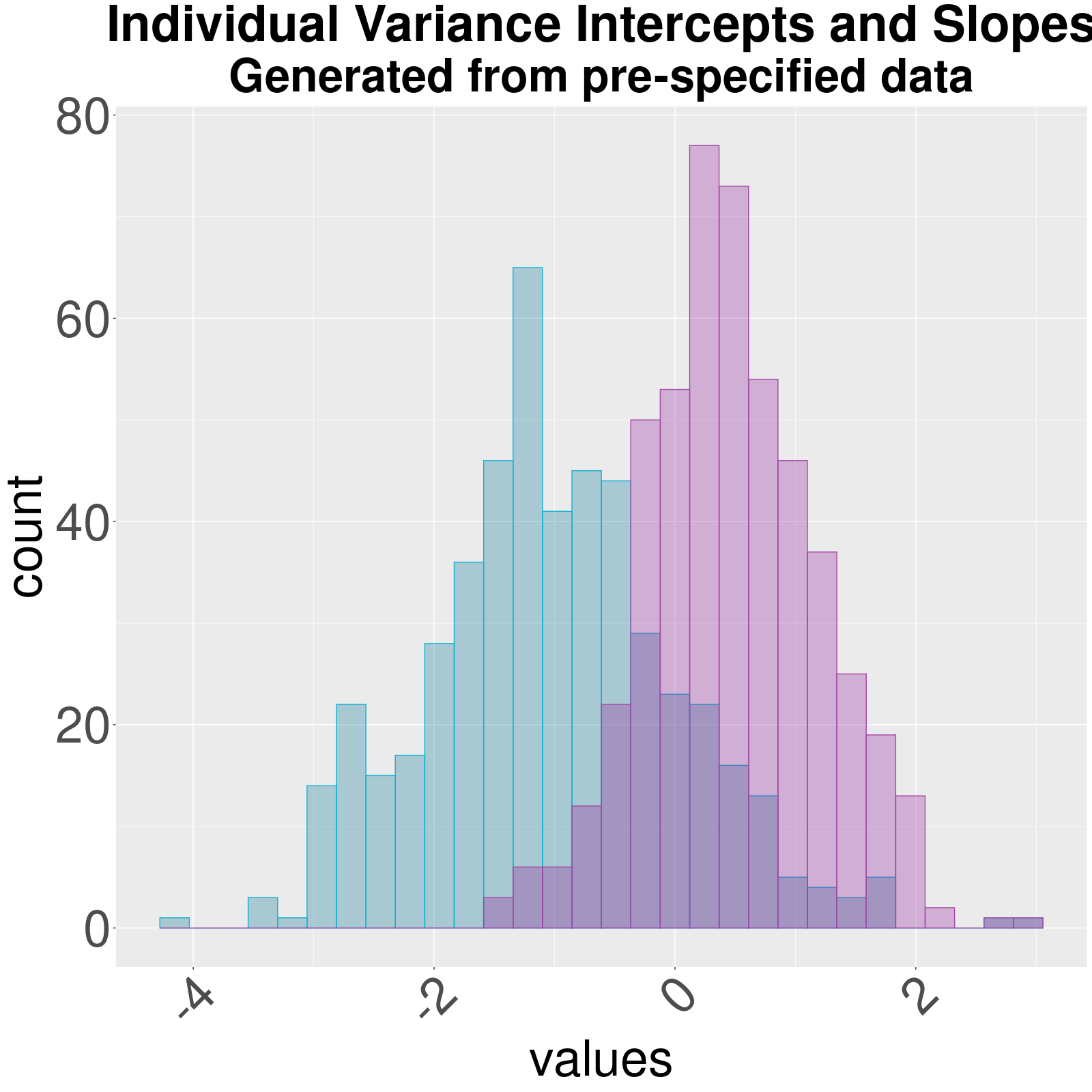
(b)

Figure 4: Individual variance intercepts (left, flatter histogram) and slopes (right, peaked histogram) and individual mean, variance and marker trajectories (line plots) for the ”high variability” simulation scenario. When the individual variability trajectory is increasing, we see that the marker trajectory has higher variability between measurements.

In the second scenario, we keep the same $\boldsymbol{\alpha},\Sigma$ values, but change $\boldsymbol{\alpha}_{s},\Sigma_{s}$ to be:

$$\boldsymbol{\alpha}_{s}=(0,0)^{{\sf T}},\Sigma_{s}=\begin{pmatrix}0.5&-0.01\\ -0.01&0.05\end{pmatrix},$$

so that the intercepts and slopes for the individual variances are smaller in magnitude. Figure 5 displays histograms of the generated individual intercepts and slopes from one simulation replicate. We will refer to this scenario as the “low-variability” (LV) case.

(a)

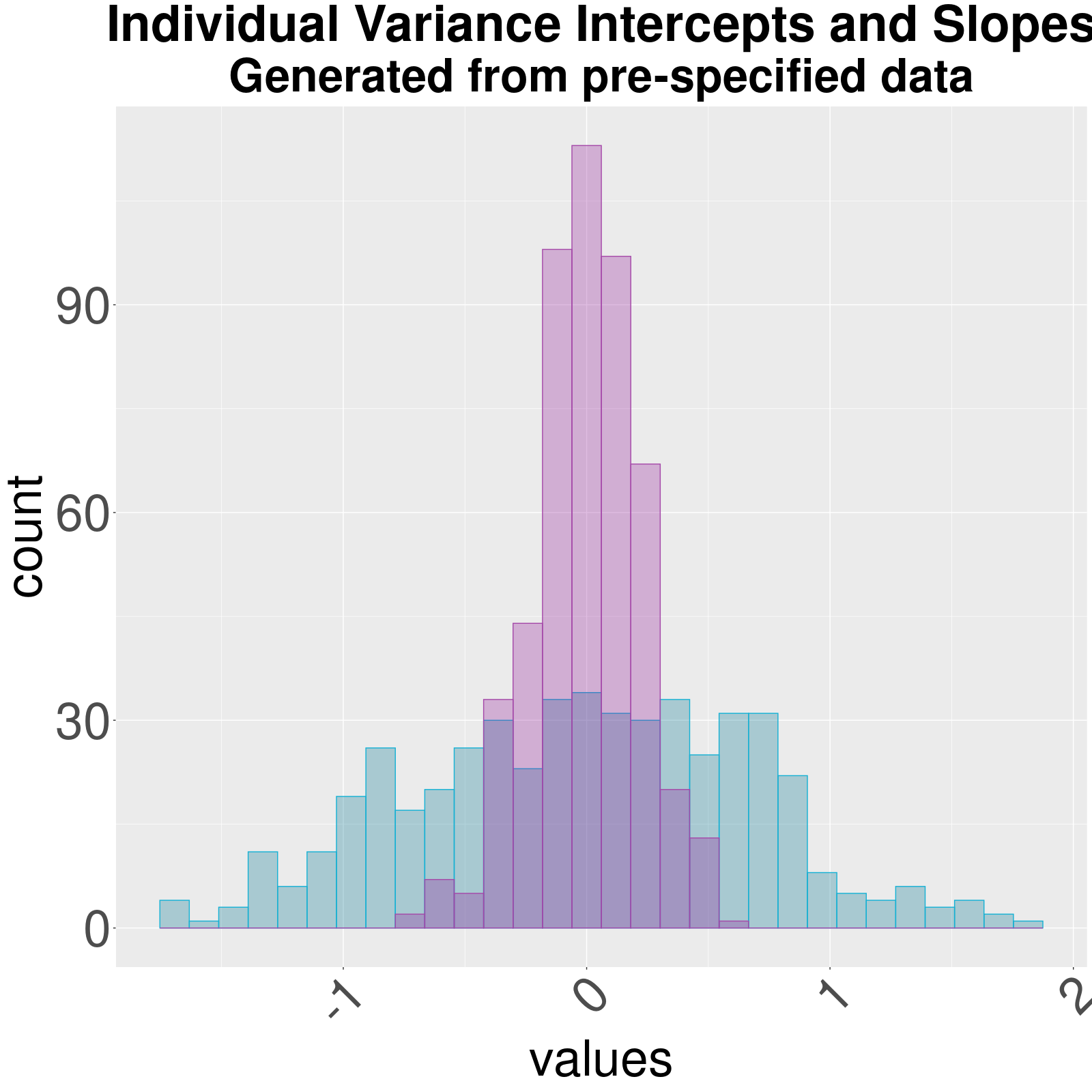
(b)

Figure 5: Histograms (left plot) of individual intercepts (flatter histogram) and slopes (peaked histogram) and individual mean, variance and predictor trajectories (line plots) for the ”low variability” simulation scenario.

$$\eta_{ij}(\mathbf{b}_{i},\bm{s}_{i})=\beta_{0}+\beta_{1}\mu_{ij}+\beta_{2}\sigma^{2}_{ij}$$

$$+(\beta_{3}+\beta_{4}\mu_{ij}+\beta_{5}\sigma^{2}_{ij})t_{ij}+a_{0i},$$

so that the marker means and variances are also interacted with time. The random intercepts $a_{0i}$ are drawn from a $\mathcal{N}(0,0.5^{2})$ (as in the previous simulation study in Section 3.1). Lastly, we set the value of the residual standard deviation of the outcome to be $\sigma=0.1$.

3.2.1 Model Comparisons

Since standard methods for longitudinal outcomes (e.g. linear mixed models) do not have functionality to model a time-varying residual error variance, we compared our model (JELO) with a time-varying variance performance against our model with a constant variance parameterization (JELO CV). For the JELO CV simulation replicates, we used the same simulated datasets generated by the time-varying variance setup described above, but we fit the model for individual variances described in Equations (3) and (4).

Truth	Scenario	Model	Bias	Coverage (%)	Average Interval Length
$\beta_{0}$ = 2	HV	JELO	0.00	96.5	0.12
	HV	JELO (CV)	0.05	68.5	0.12
	LV	JELO	0.00	95.0	0.24
	LV	JELO (CV)	0.00	93.0	0.24
$\beta_{1}$ = -1.5	HV	JELO	0.00	91.0	0.08
	HV	JELO (CV)	0.00	93.5	0.08
	LV	JELO	0.00	92.5	0.10
	LV	JELO (CV)	0.00	91.0	0.10
$\beta_{2}$ = 0.25	HV	JELO	0.00	94.5	0.15
	HV	JELO (CV)	-0.20	0.5	0.11
	LV	JELO	0.00	95.0	0.19
	LV	JELO (CV)	0.00	95.4	0.19
$\beta_{3}$ = 1	HV	JELO	0.00	98.5	0.18
	HV	JELO (CV)	-0.05	82.5	0.18
	LV	JELO	-0.01	97.5	0.06
	LV	JELO (CV)	0.00	97.0	0.06
$\beta_{4}$ =0.75	HV	JELO	0.00	95.5	0.05
	HV	JELO (CV)	0.01	82.5	0.05
	LV	JELO	0.00	95.0	0.27
	LV	JELO (CV)	-0.01	96.4	0.26
$\beta_{5}$ = -0.10	HV	JELO	0.00	96.0	0.12
	HV	JELO (CV)	0.29	0.0	0.10
	LV	JELO	0.00	99.0	0.06
	LV	JELO (CV)	0.01	96.4	0.13

Table 3: Simulation II: bias, coverage, and 95% credible interval length across 200 simulation replicates for each data scenario.

From Table 3, it is clear that when there are large individual time-varying variances, incorrectly assuming constant individual variances lead to undercoverage of all of the outcome parameters. Coverage of the coefficient for the individual variance $\beta_{2}$ and the time-variance interaction coefficient $\beta_{5}$ are essentially non-existent. However, if the individual variances are smaller, then the assumption of constant variances does not appear to result in undercoverage or substantially biased estimates of the true parameters. We can be reasonably confident that the constant variance assumption may suffice in scenarios where the the individual variances are time-varying, but not substantially different across time. However, if the time-varying variances are substantially changing across time within an indivdual, then this assumption would likely result in higher bias and substantial undercoverage of the true parameters.

4 Associations between hormone levels and hormone variabilities, and bone trajectories

We now apply our proposed model to analyze the hormone and bone trajectory data described in Section 1.1. Our outcome model formulation was specified as follows:

$$\mathbb{E}(\log_{2}(BMD_{ij}))=\beta_{0}+\beta_{1}\mu_{ij}+\beta_{2}s^{2}_{i}$$

$$+(\beta_{3}+\beta_{4}\mu_{ij}+\beta_{5}s^{2}_{i})t_{ij}+\beta_{6}BMI^{*}_{i}+\beta_{7}Age^{*}_{i}+a_{0i},$$

where $\mu_{ij}$ is the mean E2 (FSH) residual at time $t_{ij}$ from the longitudinal submodel, $s^{2}_{i}$ is the individual-level variance, $t_{ij}$ is the time to FMP for each individual woman, $BMI^{*}_{i},Age^{*}_{i}$ are the standardized BMI and baseline age values for each individual, and $a_{0i}$ is a random intercept for each woman. We also explored models with a linear random slope and quadratic random slope, but found that the estimates of the linear random slopes and the quadratic random slopes were essentially 0. Furthermore, the E2-BMD model with a quadratic random slope failed to converge. We thus concluded that a random intercept was sufficient to capture the within-individual BMD measurement correlations. The estimated variances of the random intercept in both models can be found in Tables S1 and S2 in the Supplementary Materials.

We ran two separate models, one with E2 measurements as the main biomarker measurement of interest and one with FSH measurements as the main predictor of interest. For the longitudinal predictor, we used the E2 (FSH) measurement obtained at the previous visit to predict BMD at the following visit. This is to better capture how differences in E2 at an earlier time may be associated with BMD declines later, rather than analyzing E2 and BMD values at the same timepoint.

The models in the following sections used a time-invariant individual variance for the predictor hormone. We also attempted to fit a time-varying individual variance component (see Simulation 3.2) on the SWAN dataset, but encountered severe model convergence issues. We suspected that the number of timepoints in the dataset was not large enough to capture a time-varying variance trend.

4.1 E2 Predictor Model

In this model, we included interaction between the (lagged) estimated E2 residual and time to FMP when the BMD measurement was collected, and the interaction between E2 variability and time to FMP. Table 4 displays the estimated posterior means and 95% credible intervals for the outcome coefficients.

Variable	Post. Mean	95% CrI
Predicted E2	29.46	(25.25,35.00)
E2 Var.	-2.38	(-6.76, 2.05)
Time to FMP	-0.79	(-1.12, -0.49)
Time to FMP x Predicted E2	0.31	(0.12, 0.58)
Time to FMP x E2 Var.	0.21	(-0.01,0.46 )
BMI	12.21	(11.00, 13.41)
Age	0.11	(-0.36, 0.57)

Table 4: Estimated posterior means and 95% credible intervals for the E2-BMD model with time interactions. All estimated posterior means and 95% CrI values have been multiplied by $10^{2}$.

The predicted E2 residual at the visit before FMP was significantly associated with BMD at FMP (i.e., when $t_{ij}$ = 0). The interpretation of the coefficient is that for women with a 1 unit (mg/l) higher predicted E2 residual at the visit before FMP, there was an average corresponding $(2^{0.3474}-1)\times 100\%=22.8\%(19.1\%,27.5\%)$ higher BMD at FMP. This effect was slightly moderated by time, since the coefficient for the interaction of predicted E2 and time is negative. However, the credible interval for the estimated interaction effect of time and E2 contains 0, meaning that the estimated effect of E2 on BMD does not significantly change over time. This is also evident from Figure 6, where the estimated slopes of the BMD trajectories do not change over the menopausal transition.

When predicted E2 is at the population average, an additional one year was associated with a $(1-2^{-0.0079})\times 100\%=-0.54\%(-0.77\%,-0.34\%)$ change in BMD. If we hold predicted E2 constant, then each additional year is associated with a $(1-2^{-0.0079}\times 2^{0.0031})\times 100\%=-0.33\%(-0.70\%,0.06\%)$ decrease in predicted BMD.

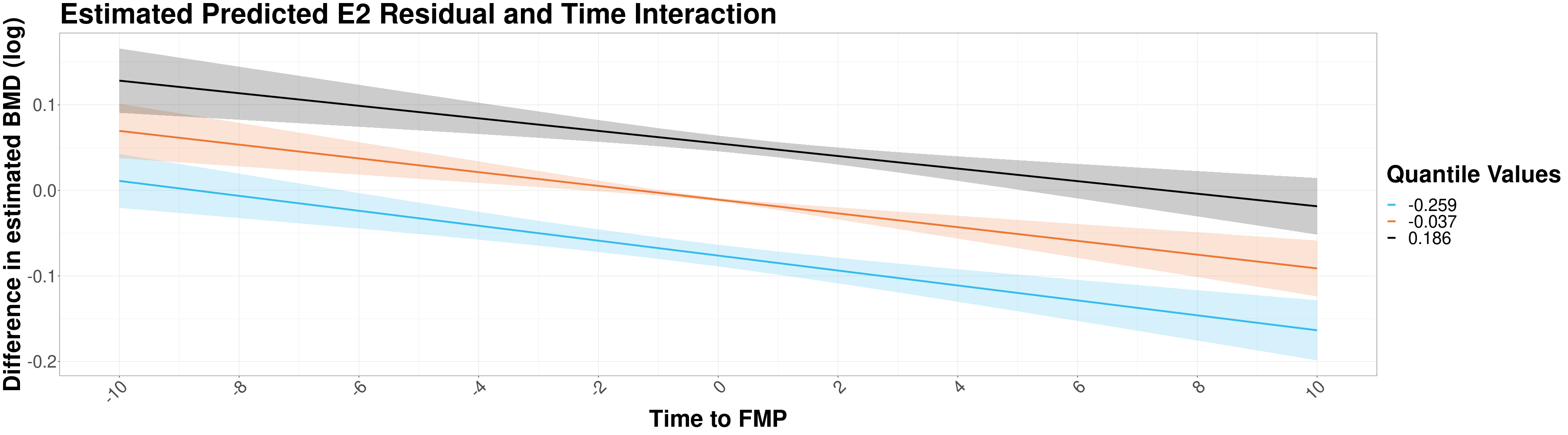
Figure 6: Plots of predicted E2 residuals and time interaction for the BMD outcome model. The solid lines represent the 25th, 50th, and 75th quantile values of the E2 variable, along with the prediction band for this value.

Higher E2 variability at FMP was negatively associated with BMD; a one unit increase in E2 variance was associated with a $(1-2^{-0.0238})\times 100\%=-1.6\%(-4.74\%,1.43\%)$ change in BMD. However, since the 95% CrIs contained 0, we cannot say that this relationship was statistically significant. The interaction term for E2 variance and time to FMP was also not significant.

Finally, baseline BMI was positively associated with BMD, indicating that women with higher BMI tended, on average, to have higher $8.8\%$ BMD ($8.0\%,9.74\%$), holding all else constant. Baseline age, however, was not significantly associated with BMD.

4.2 FSH Predictor Model

Table 5 displays the estimated posterior means and 95% credible intervals for the FSH model outcome coefficients. Predicted FSH residual at the visit before FMP was significantly associated with BMD at FMP (when $t_{ij}=0$). For women with a 1 unit (pg/mL) higher predicted FSH residual at the visit before FMP, there was an average corresponding $(1-2^{-0.2700})\times 100\%=-17.1\%(-18.7\%,-15.4\%)$ lower BMD at FMP. When predicted FSH is at the population average, an additional one year was associated with a $(1-2^{-0.0028})\times 100\%=-0.19\%(-0.33\%,-0.06\%)$ change in BMD. The FSH and time interaction was also significant and indicated that the association between mean FSH and BMD becomes amplified over time. If we hold predicted FSH constant, then each additional year was associated with a $(1-(2^{-0.0028}\times 2^{-0.0097})\times 100\%=-0.86\%(-1.15\%,-0.57\%)$ change in predicted BMD residual. This can also be seen in Figure 7, where the estimated BMD trajectories tend to diverge after FMP.

Variable	Post. Mean	95% CrI
Predicted FSH	-27.00	(-29.83, -24.25)
FSH Var.	0.80	(-4.29, 5.95)
Time to FMP	-0.28	(-0.48, -0.09)
Time to FMP x Predicted FSH	-0.97	(-1.20, -0.74)
Time to FMP x FSH Var.	0.38	(0.12, 0.64)
BMI	9.86	(8.58, 11.24)
Age	-0.22	(-0.70, 0.29)

Table 5: Estimated posterior means and 95% credible intervals for the FSH-BMD model with time interactions. All estimated posterior means and 95% CrI values have been multiplied by $10^{2}$.

FSH variability at FMP was not significantly associated with BMD. The interaction term, however, between variability and time to FMP was significant. Holding FSH variability constant, a one year increase in time to FMP is associated with a $(1-2^{-0.0028}\times 2^{0.0038})=0.07\%(-0.25\%,0.38\%)$ change in BMD. Since this interaction term has a positive sign, this indicates that the association of FSH variability with BMD is moderated over time. The bottom plot in Figure 7 shows this moderating effect where the estimated difference in BMD trajectories converge around 8 years post FMP.

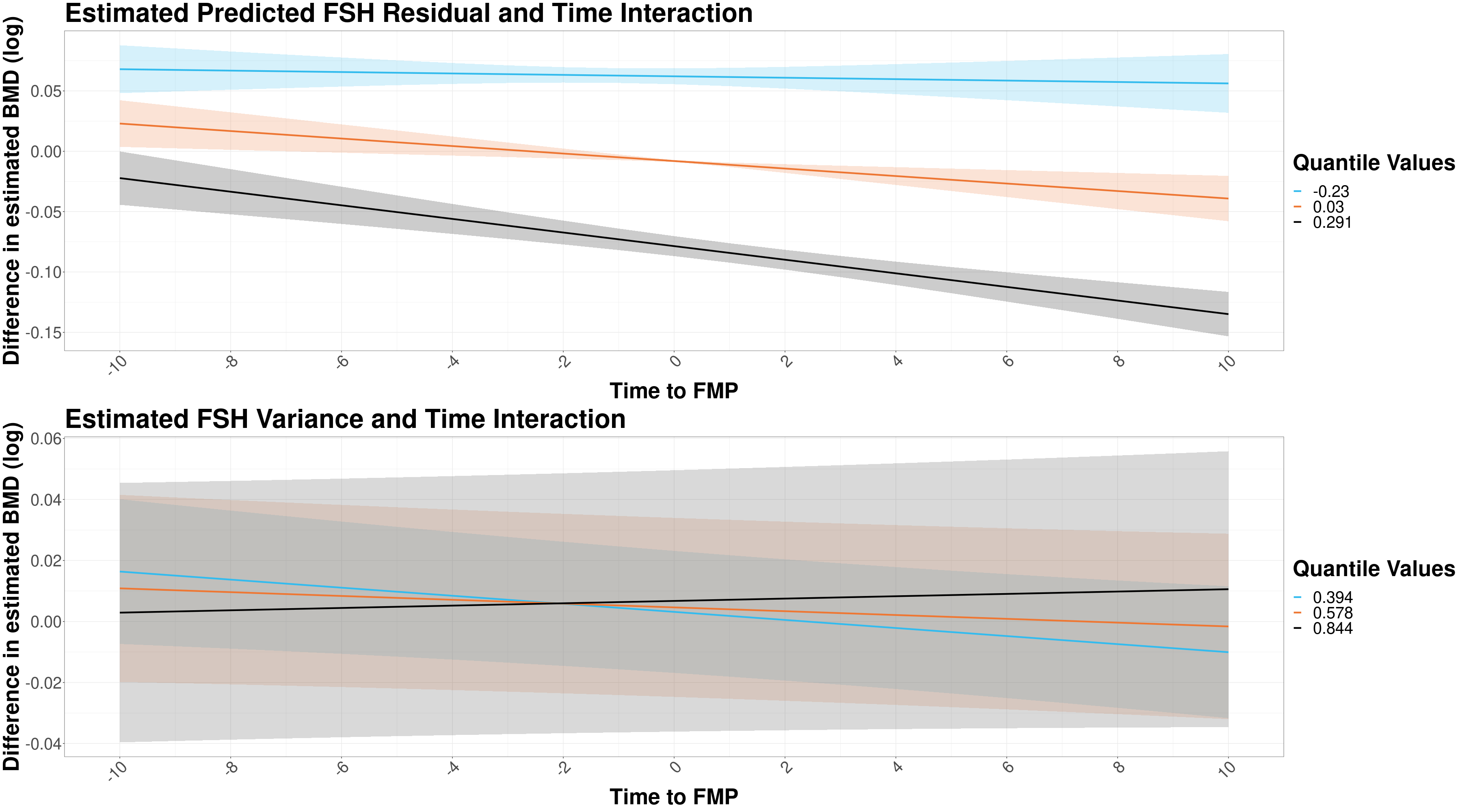
Figure 7: Plots of predicted FSH and time interaction (top figure) and FSH variance and time interaction (bottom figure) for the BMD outcome model. The solid lines represent the 25th, 50th, and 75th quantile values of the FSH variable, along with the prediction band for this value. We can see the moderating effect of the variance-time interaction term as the BMD residual trajectories converge at around 7 years post-FMP.

Finally, as in the E2 predictor model, baseline BMI was significantly associated with BMD. Women with higher BMI values tended to have higher BMD values, holding all else constant. This is consistent with the literature on associations between body size and BMD in adult women (Salamat and others, 2013). Baseline age was not significantly associated with BMD.

5 Discussion

Maintaining bone health in women is particularly important with aging. Given that BMD declines accelerate during the menopausal transition, much attention has been given to this life stage in terms of bone health prevention (Finkelstein and others, 2008). Additionally, the menopausal transition is a period of time with large changes in sex hormone levels and increased variability. Although much research has evaluated associations between sex hormone levels and BMD, there is still a lack of understanding of how hormone variabilities may affect BMD loss in women undergoing menopause.

In our analyses, we found that higher mean E2 was associated with higher average predicted BMD, which supports the hypothesis that higher levels of E2 are protective against BMD loss, and support bone health during the midlife. Conversely, higher FSH was associated with lower average BMD, which suggests that higher levels of FSH may negatively affect bone health in the midlife for women. These findings are consistent with the literature on the relationship between E2 and FSH levels and BMD outcomes in women during the midlife (Zaidi and others, 2018; Park and others, 2021).

Furthermore, we found that FSH variability was significantly associated with higher predicted BMD loss across the menopausal transition, with a one-unit higher FSH variability at FMP being associated with a 3.2% lower BMD. We did not find a similar relationship between BMD and E2 variability. This suggests that FSH variability is more strongly predictive of BMD trajectories in menopausal women than E2 variability. These findings should motivate further research into the role of FSH variability on BMD declines to more fully understand the relationship between individual variances of hormones and women’s BMD trajectories.

Our analysis had a few limitations. As noted in the introduction, BMD has a nonlinear rapid decrease as women approach the menopausal transition, and then stabilizes around 2-5 years after FMP. Originally, we attempted to fit an outcome model with a linear spline on time to FMP, with knots at 2 years before and after FMP. This model had trouble converging for both hormone predictors. In particular, the coefficients that represented the mean and variance interacted with the spline on time to FMP failed to converge. To address this, we decided to remove the nonlinear BMD trend by using the individual BMD residuals as the main outcome of interest; this left subject-level trends that could be modeled linearly. Additionally, as mentioned in Section 4, when we attempted to fit a linear time-varying variance on the SWAN dataset, the model had convergence problems, most likely due to the insufficient number of timepoints necessary to capture a time-varying variance trend.

Future Work

Even though BMD is the standard metric of choice used to evaluate bone health, some have cautioned against solely relying on BMD to measure bone health. Prentice and others (1994) argued that BMD should not be used in epidemiological studies. Since the formula for BMD assumes a constant proportional relationship between bone area and BMC (bone mineral content), this can lead to spurious correlations between BMD and health outcomes when the relationship between BMC and bone area is not directly proportional. “If BMD is used when the relationship between BMC and BA [bone area] is not one of simple direct proportion, part of its variation within a population will be due to differences in bone size between individuals.” Now that we have looked at the association between hormone variability and BMD, the next question of interest would be to understand if these associations are also present with women’s BMC and bone area trajectories.

The SWAN study has collected women’s femoral neck BMC (g) measurements and femoral neck area (cm²) measurements visits, but due to changes in the DXA collection machines over the course of the study, these measurements are not yet appropriately calibrated for longitudinal analyses. When the calibrated measurements become available, we plan to apply our model to BMC trajectories and bone area trajectories. Another possible extension of the model would be to simultaneously model both BMC and bone area trajectories as a multivariate outcome, rather than separately analyzing each variable.

An interesting future area of research could be to model complex formulation of the individual variances. In particular, decomposing individual time-varying variances into short-term and long-term trends may be of scientific interest for epidemiologists and physicians. To explore these higher-order trends and obtain sufficiently stable estimates of the variance trends, we will likely need a larger dataset than the one available.

Finally, our joint model is specified for one longitudinal marker, but this could be extended to multiple longitudinal markers by specifying $\mathbf{B}_{i}=[\bm{b}_{i1},...,\bm{b}_{iQ}]^{{\sf T}}$, where $Q$ is the number of markers, and a $Q\times Q$ variance-covariance matrix $\mathbf{S}_{i}$ for each individual. This extension would have several considerations. The computation cost of estimating $\mathbf{S}_{i}$ would grow non-linearly as $Q$ increases. Additionally, if we wanted to model both a mean regression and covariance regression (e.g. time-varying covariance matrices) in the predictor model, then this would further increase the computational burden of estimating the model.

6 Data Availability

We provide code to replicate our simulation studies and data analysis at the Github repository linked here: https://github.com/realirena/jelo/. We are unable to make the SWAN dataset publicly available, due to its clinical and biomedical nature. To request access to the SWAN dataset, we refer the reader to: https://www.swanstudy.org/swan-research/data-access/.

References

- Alswat (2017) Alswat, Khaled A. (2017). Gender disparities in osteoporosis. Journal of Clinical Medicine Research 9(5), 382–387.
- Carpenter and others (2017) Carpenter, Bob, Gelman, Andrew, Hoffman, Matthew D., Lee, Daniel, Goodrich, Ben, Betancourt, Michael, Brubaker, Marcus, Guo, Jiqiang, Li, Peter and Riddell, Allen. (2017). Stan: A probabilistic programming language. Journal of Statistical Software 76, 1–32.
- Chin (2018) Chin, Kok-Yong. (2018). The relationship between follicle-stimulating hormone and bone health: Alternative explanation for bone loss beyond oestrogen? International Journal of Medical Sciences 15(12), 1373–1383.
- Diggle and others (2013) Diggle, Peter, Heagerty, Patrick, Liang, Kung-Yee and Zeger, Scott. (2013). Analysis of Longitudinal Data, Second Edition edition., Oxford Statistical Science Series. Oxford University Press.
- Ebeling and others (1996) Ebeling, P. R., Atley, L. M., Guthrie, J. R., Burger, H. G., Dennerstein, L., Hopper, J. L. and Wark, J. D. (1996). Bone turnover markers and bone density across the menopausal transition. The Journal of Clinical Endocrinology and Metabolism 81(9), 3366–3371.
- Elliott and others (2012) Elliott, Michael R., Sammel, Mary D. and Faul, Jessica. (2012). Associations between variability of risk factors and health outcomes in longitudinal studies. Statistics in Medicine 31, 2745–2756.
- Finkelstein and others (2008) Finkelstein, Joel S., Brockwell, Sarah E., Mehta, Vinay, Greendale, Gail A., Sowers, MaryFran R., Ettinger, Bruce, Lo, Joan C., Johnston, Janet M., Cauley, Jane A., Danielson, Michelle E. and others. (2008). Bone mineral density changes during the menopause transition in a multiethnic cohort of women. The Journal of Clinical Endocrinology and Metabolism 93(3), 861–868.
- Gambacciani and Levancini (2014) Gambacciani, Marco and Levancini, Marco. (2014). Hormone replacement therapy and the prevention of postmenopausal osteoporosis. Przeglad Menopauzalny (Menopause Review) 13(4), 213–220.
- Gao and others (2022) Gao, Feng, Luo, Jingqin, Liu, Jingxia, Wan, Fei, Wang, Guoqiao, Gordon, Mae and Xiong, Chengjie. (2022). Comparing statistical methods in assessing the prognostic effect of biomarker variability on time-to-event clinical outcomes. BMC medical research methodology 22(1), 201.
- Gelman (2006) Gelman, Andrew. (2006). Prior distributions for variance parameters in hierarchical models (comment on article by Browne and Draper). Bayesian Analysis 1, 515–534.
- Gourlay and others (2011) Gourlay, M. L., Preisser, J. S., Hammett-Stabler, C. A., Renner, J. B. and Rubin, J. (2011). Follicle-stimulating hormone and bioavailable estradiol are less important than weight and race in determining bone density in younger postmenopausal women. Osteoporosis international: a journal established as result of cooperation between the European Foundation for Osteoporosis and the National Osteoporosis Foundation of the USA 22(10), 2699–2708.
- Greendale and others (2019) Greendale, Gail A., Sternfeld, Barbara, Huang, MeiHua, Han, Weijuan, Karvonen-Gutierrez, Carrie, Ruppert, Kristine, Cauley, Jane A., Finkelstein, Joel S., Jiang, Sheng-Fang and Karlamangla, Arun S. (2019). Changes in body composition and weight during the menopause transition. JCI Insight 4, e124865.
- Greene (2005) Greene, Willam. (2005). Fixed and random effects in stochastic frontier models. Journal of Productivity Analysis 23(1), 7–32.
- Harlow and others (2000) Harlow, S. D., Lin, X. and Ho, M. J. (2000). Analysis of menstrual diary data across the reproductive life span applicability of the bipartite model approach and the importance of within-woman variance. Journal of Clinical Epidemiology 53, 722–733.
- Hickey and others (2016) Hickey, Graeme L., Philipson, Pete, Jorgensen, Andrea and Kolamunnage-Dona, Ruwanthi. (2016). Joint modelling of time-to-event and multivariate longitudinal outcomes: recent developments and issues. BMC Medical Research Methodology 16(1), 117.
- Hunter and Sambrook (2000) Hunter, D. J. and Sambrook, P. N. (2000). Bone loss. epidemiology of bone loss. Arthritis Research 2(6), 441–445.
- Ji and Yu (2015) Ji, Meng-Xia and Yu, Qi. (2015). Primary osteoporosis in postmenopausal women. Chronic Diseases and Translational Medicine 1(1), 9–13.
- Jiang and others (2015) Jiang, Bei, Elliott, Michael R., Sammel, Mary D. and Wang, Naisyin. (2015). Joint modeling of cross-sectional health outcomes and longitudinal predictors via mixtures of means and variances. Biometrics 71, 487–497.
- Laird and Ware (1982) Laird, Nan M. and Ware, James H. (1982). Random-effects models for longitudinal data. Biometrics 38(4), 963–974.
- Lewandowski and others (2009) Lewandowski, Daniel, Kurowicka, Dorota and Joe, Harry. (2009). Generating random correlation matrices based on vines and extended onion method. Journal of Multivariate Analysis 100, 1989–2001.
- Liang and Zeger (1986) Liang, Kung-Yee and Zeger, Scott L. (1986). Longitudinal data analysis using generalized linear models. Biometrika 73(1), 13–22.
- Marshall and others (1996) Marshall, D., Johnell, O. and Wedel, H. (1996). Meta-analysis of how well measures of bone mineral density predict occurrence of osteoporotic fractures. BMJ (Clinical research ed.) 312(7041), 1254–1259.
- McNeish and Matta (2018) McNeish, Daniel and Matta, Tyler. (2018). Differentiating between mixed-effects and latent-curve approaches to growth modeling. Behavior Research Methods 50(4), 1398–1414.
- Park and others (2021) Park, Young-Min, Jankowski, Catherine M., Swanson, Christine M., Hildreth, Kerry L., Kohrt, Wendy M. and Moreau, Kerrie L. (2021). Bone mineral density in different menopause stages is associated with follicle stimulating hormone levels in healthy women. International Journal of Environmental Research and Public Health 18(3), 1200.
- Pinheiro and others (2022) Pinheiro, José, Bates, Douglas and R Core Team. (2022). nlme: Linear and Nonlinear Mixed Effects Models. R package version 3.1-157.
- Prentice and others (1994) Prentice, A, Parsons, T J and Cole, T J. (1994). Uncritical use of bone mineral density in absorptiometry may lead to size-related artifacts in the identification of bone mineral determinants. The American Journal of Clinical Nutrition 60(6), 837–842.
- Randolph and others (2011) Randolph, John F., Zheng, Huiyong, Sowers, MaryFran R., Crandall, Carolyn, Crawford, Sybil, Gold, Ellen B. and Vuga, Marike. (2011). Change in follicle-stimulating hormone and estradiol across the menopausal transition: Effect of age at the final menstrual period. The Journal of Clinical Endocrinology and Metabolism 96, 746–754.
- Randolph and others (2004) Randolph, John F. Jr., Sowers, MaryFran, Bondarenko, Irina V., Harlow, Siobán D., Luborsky, Judith L. and Little, Roderick J. (2004). Change in estradiol and follicle-stimulating hormone across the early menopausal transition: Effects of ethnicity and age. The Journal of Clinical Endocrinology & Metabolism 89, 1555–1561.
- Recker and others (2000) Recker, R, Lappe, J, Davies, K and Heaney, R. (2000). Characterization of perimenopausal bone loss: a prospective study. Journal of Bone and Mineral Research: The Official Journal of the American Society for Bone and Mineral Research 15(10), 1965–1973.
- Riggs and Melton (1992) Riggs, B. Lawrence and Melton, L. Joseph. (1992). The prevention and treatment of osteoporosis. New England Journal of Medicine 327(9), 620–627.
- Salamat and others (2013) Salamat, Mohammad Reza, Salamat, Amir Hossein, Abedi, Iraj and Janghorbani, Mohsen. (2013). Relationship between weight, body mass index, and bone mineral density in men referred for dual-energy x-ray absorptiometry scan in isfahan, iran. Journal of Osteoporosis 2013, 205963.
- Sirola and others (2003) Sirola, Joonas, Kröger, Heikki, Honkanen, Risto, Jurvelin, Jukka S., Sandini, Lorenzo, Tuppurainen, Marjo T., Saarikoski, Seppo and OSTPRE Study Group. (2003). Factors affecting bone loss around menopause in women without HRT: a prospective study. Maturitas 45(3), 159–167.
- Sowers and others (2000) Sowers, MARYFRAN, Crawford, SYBIL L., Sternfeld, BARBARA, Morganstein, DAVID, Gold, ELLEN B., Greendale, GAIL A., Evans, Denis A., Neer, ROBERT, Matthews, KAREN, Sherman, SHERRY, Lo, ANNIE, Weiss, GERSON and others. (2000). Design, survey sampling and recruitment methods of SWAN: A multi-center, multi-ethnic, community-based cohort study of women and the menopausal transition. In: Menopause: biology and pathobiology, Volume 175. Academic Press, pp. 175–188.
- Stan Development Team (2020) Stan Development Team. (2020). RStan: the R interface to Stan. R package version 2.21.2.
- Uhler and others (2005) Uhler, M. L., Rao, R. P., Beltsos, A. N., Grotjan, H. and Lifchez, A. S. (2005). High intercycle variability of day 3 FSH levels is useful for predicting ovarian responses but not pregnancy outcomes in IVF. Fertility and Sterility 84, S265. Publisher: Elsevier.
- Vehtari and others (2021) Vehtari, Aki, Gelman, Andrew, Simpson, Daniel, Carpenter, Bob and Bürkner, Paul-Christian. (2021). Rank-normalization, folding, and localization: An improved rˆ for assessing convergence of MCMC (with discussion). Bayesian Analysis 16, 667–718. Publisher: International Society for Bayesian Analysis.
- Zaidi and others (2018) Zaidi, Mone, Lizneva, Daria, Kim, Se-Min, Sun, Li, Iqbal, Jameel, New, Maria I, Rosen, Clifford J and Yuen, Tony. (2018). FSH, bone mass, body fat, and biological aging. Endocrinology 159(10), 3503–3514.
- Zhang and others (2022) Zhang, Ziwei, Rohloff, Corissa T. and Kohli, Nidhi. (2022). Model fit indices for random effects models: Translating model fit ideas from latent growth curve models. Structural Equation Modeling: A Multidisciplinary Journal 0(0), 1–9.