Dark I-Love-Q

Abstract

For neutron stars, there exist universal relations insensitive to the equation of states, the so called I-Love-Q relations, which show the connections among the moment of inertia, tidal Love number and quadrupole moment. In this paper, we show that these relations also applies to dark stars, bosonic or fermionic. The relations can be extended to a higher range of the variables, as those curves all approximate the ones generated by a polytropic equation of state, when taking the low density (pressure) limit.

I Introduction

Since the first observation of gravitational waves (GW) from two inspiral black holes (BH) LIGOScientific:2016aoc , we enter the era of multi-messenger astronomy. Besides BH, GW also serve as excellent observatories for other compact stars like neutron stars (NS) TheLIGOScientific:2017qsa ; Abbott:2018wiz , and they can read off not only the binary masses but also the tidal deformability, which could further infer the radii. While for traditional observation method, the NS radius has to be calculated by X-ray burst or thermodynamics, with an error of some $20\%$. The data from GW will enhance the accuracy of our estimation about the radius. However, to perform this task, the exact equation of state (EoS) of NS is needed, which is now still an open question and most of the mainstream EoS models like SLy4 Douchin:2001sv , APR4 Akmal:1998cf etc. have lots of parameters. Though there are some other theoretically derived ones with only one parameter like the MIT bag modelROSENHAUER1992630 or from holographic QCD Zhang:2019tqd , they are less realistic. Here by realistic it means that the EoS should describe a star with mass, radius and tidal deformability comparable to the observation data range. With different EoS, the deduced NS mass, radius and tidal Love number (TLN) vary and show strong dependence. However, in 2013 some universal relations insensible to EoS was found Yagi:2013bca ; Yagi:2013awa , which showed the relations among the (reduced) momentum of Inertia I, TLN and quadrupole moment Q. These are called the I-Love-Q relations. They show that, any two of the three variables form a function which is almost independent of the EoS applied, as long as it is realistic. Thus I-Love-Q relations can serve as a quick investigation of the observation data, to infer one of the trio from another, or to test the validity of general relativity.

In the astronomical observation for NS and BH, there are so-called gap events distinguished by star masses, with the lower gap between $2.5$ and $5$ $M_{\odot}$ (solar mass), and the higher gap between $80$ and $150$ $M_{\odot}$. For the lower gap, 2.5 $M_{\odot}$ is too heavy for an NS, while $5$ is in general too light for a stellar BH, unless it is a primordial BH, or a remnant of other NS merger event. For the higher gap, this range is not allowed for stellar BH, so the most possibility is primordial BH, or a remnant of other BH merger. Nonetheless, there might be another candidate for gap events, the dark stars (DS). Dark matter (DM) is generally believed to be dispersed, but considering the fact that it occupies $27\%$ of the universe energy, much larger than the $5\%$ contribution from normal matter, we cannot exclude the possibility that it could form dense stars. The star formation might be through Bondi accretion Bondi:1944jm ; Bondi:1952ni ; Ruffert:1993wi ; Ruffert:1993wm or other process, which we will not touch here and leave for the future work.

If DS do exist, then what are their EoS? Do they satisfy similar I-Love-Q relations or not? There are indeed many DM models, fermionic or bosonic, and the corresponding EoS can be extracted in principle. However, usually this is not an easy process Colpi:1986ye , where numerical approximations or shooting method etc. have to be applied. For BS, in Zhang:2020dfi ; zhang2023dark a new approach using isotropic limit is applied, then the EoS for different models can be systematically obtained. Although it is called a "limit", this limit is also a necessary condition to use the Tolman-Oppenheimer-Volkoff (TOV) equations anyway, so it is actually an accurate analytic approach. In this paper, we calculate the I-Love-Q relation for DS, using the BS EoS obtained in zhang2023dark , and FS EoS in Kouvaris:2015rea .Those for NS are also reproduced as references. We find that DS also enjoy similar I-Love-Q relation, and in fact that their curves coincide with the NS case. This is also interesting in the sense that I-Love-Q relation is more universal than expected, which applies to a large range of compact star (one may try white dwarfs to see what happens). One interpretation for why this happens is, the I-Love-Q variables are mainly affected by the outer layer of the stars, which means the energy density $\rho$ and pressure $p$ are small, while in this limit all those EoS become alike.

The organization of the paper is as follows. Section 2 introduces the EoS used, and section 3 shows the extended I-Love-Q relations for both DS and NS. We conclude in section 4. In the appendix, we review the method to calculate the I-Love-Q variables.

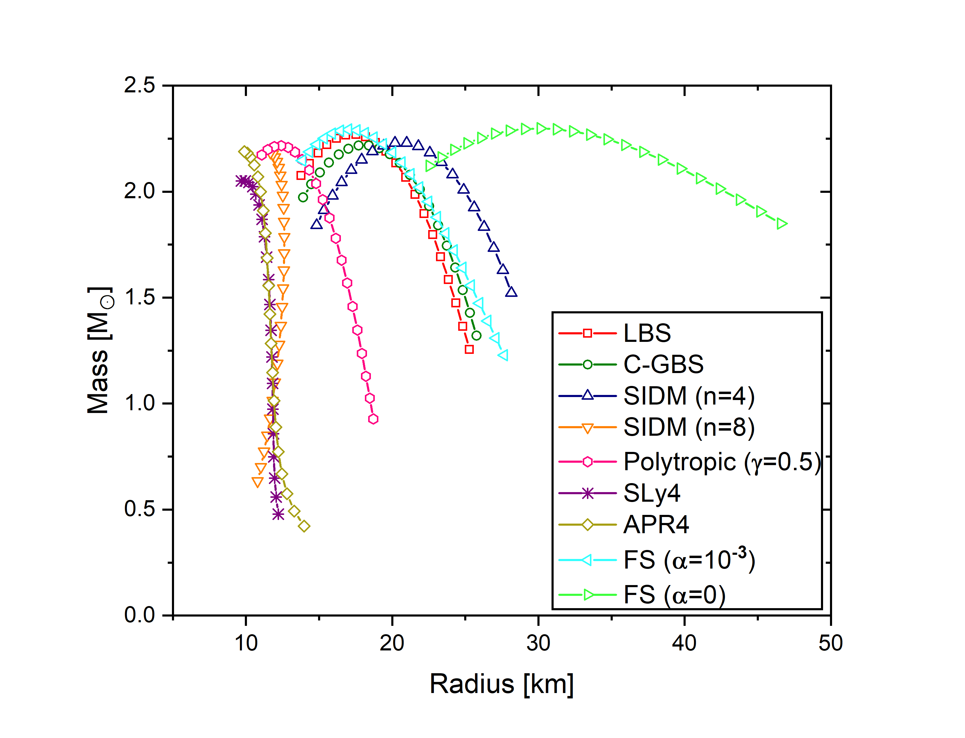
Figure 1: Mass-radius relations of 4 BS models, 2 FS models and 3 NS models.

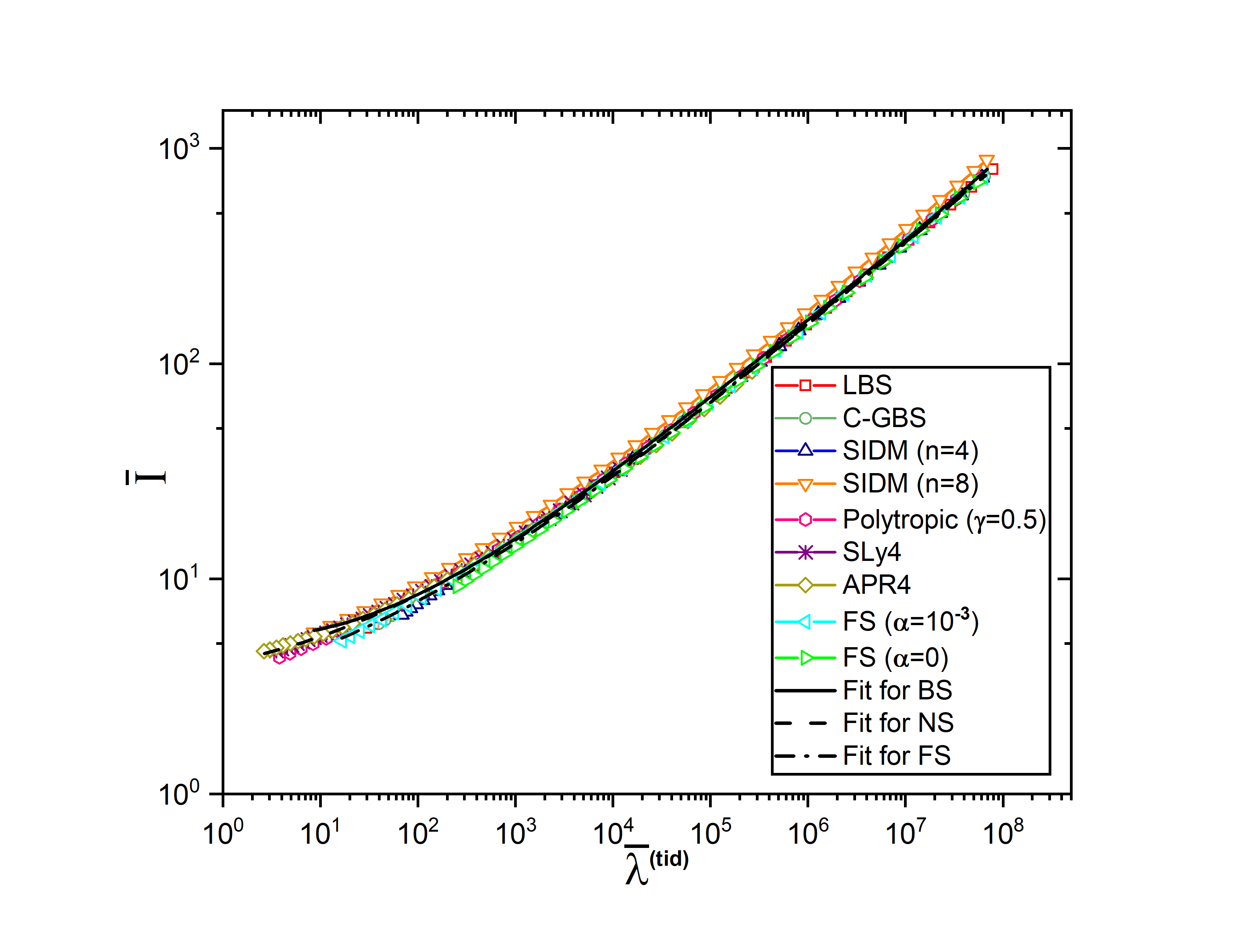
Figure 2: I-Love relations of 4 BS models, 2 FS models and 3 NS models. The black solid line refers to the fitting for BS, the black dotted line for FS, and the black dashed line represents the fitting for NS.

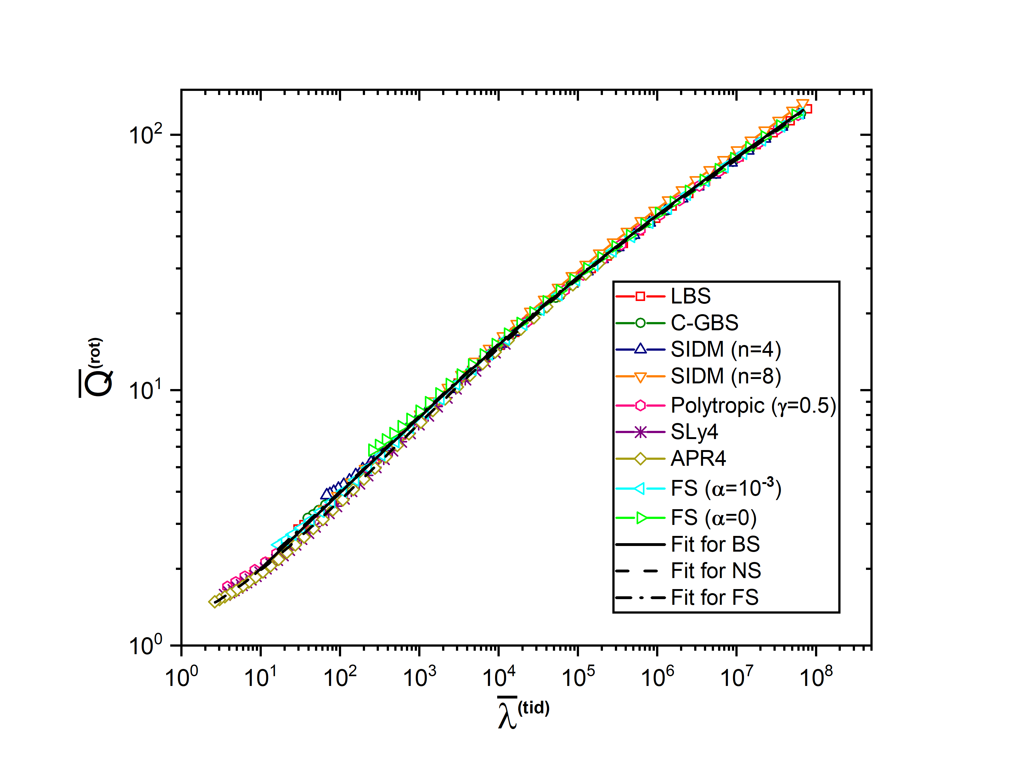
Figure 3: Q-Love relations of 4 BS models, 2 FS models and 3 NS models. The meanings of different lines are the same as those in Fig.2.

II Equation of State

In order to derive the rotating-induced and tidal-induced effects of relativistic stars, we should set the EoS first. Due to the lack of observation evidence, various dark matter models are proposed. Based on the properties of component particles, these models can be classified into FS and BS. In the formation of compact stars, the degenerate pressure through fermions prevents the FS from gravitational collapsing while BS rely on the self-interaction. Yet for FS to have a considerable size, self-interaction should also be introduced.

For NS, we apply two widely used EoS models, SLy4 and APR4, together with a simple polytropic model, $\rho=\kappa p^{\gamma}$ , with $\gamma=\frac{1}{2}$ .

For DS, we consider four different self-interacting dark matter (SIDM) models, with three bosonic zhang2023dark and one fermionic Kouvaris:2015rea . The first one describes BS with a scalar potential $V_{n}(\phi)=\frac{m^{2}}{2}|\phi|^{2}+\frac{\lambda_{n}}{n\Phi^{n-4}_{0}}|\phi|^{n}$, where $\lambda_{n}$ is a dimensionless coupling constant and $\Phi_{0}$ is a constant of the same dimension with the potential $\phi$ PhysRevLett.57.2485 . After applying the isotropic limit method, The corresponding EoS is abstracted zhang2023dark

$$\rho=\frac{n+2}{n-2}p+K_{n}p^{\frac{2}{n}},$$ (1)

where $K_{n}=(\frac{2n}{n-2})^{\frac{2}{n}}(\frac{m^{2}M_{pl}^{2}}{4\pi\Lambda_{n}})^{1-\frac{2}{n}}$ with $\Lambda_{n}=(\lambda_{n}\frac{\Phi_{0}^{2}}{m^{2}})^{\frac{2}{n-2}}\frac{M_{pl}^{2}}{\Phi_{0}^{2}}$, where $M_{pl}$ means the Planck mass. It requires $\Lambda_{n}\gg 1$ when achieving the isotropic limit. It is easy to see when $p\to 0$, this EoS approaches a polytropic one with with $\gamma=\frac{2}{n}$.

The second model is Liouville field associating with the potential $V(\phi)=\frac{m^{2}}{2\varepsilon^{2}}[e^{\varepsilon^{2}|\phi|^{2}}-1]$ and the corresponding EoS is zhang2023dark

$$\begin{split}\rho=K(\eta^{2}e^{\eta^{2}}+e^{\eta^{2}}-1),\\ p=K(\eta^{2}e^{\eta^{2}}-e^{\eta^{2}}+1),\end{split}$$ (2)

where $\eta$ is an adjustable parameter and $K=\frac{m^{2}M_{pl}^{2}}{4\pi\Lambda}$ with $\Lambda=\varepsilon M_{pl}$. For the isotropic limit, just as $\Lambda_{n}$, $\Lambda\gg 1$ is necessary. When $p\to 0$, this EoS approaches $\rho\propto p^{\frac{1}{2}}$.

The last bosonic model is cosh-Gordon field with $V(\phi)=\frac{m^{2}}{\varepsilon^{2}}[\cosh(\varepsilon\sqrt{|\phi|^{2}})-1]$. EoS has the formula zhang2023dark

$$\begin{split}\rho=K(\frac{1}{2}\eta\sinh\eta+\cosh\eta-1),\\ p=K(\frac{1}{2}\eta\sinh\eta-\cosh\eta+1),\end{split}$$ (3)

where $K$ has the same definition with the one in Eq.(3) and the isotropic limit condition is invariant for $\Lambda$. When $p\to 0$, this EoS also approaches $\rho\propto p^{\frac{1}{2}}$.

For fermionic models, we apply the EoS from Kouvaris:2015rea , considering the Yukawa potential $V={\alpha\over r}\exp(-m_{\phi}r)$, with $\alpha$ the dark fine structure constant and $m_{\phi}$ the mediator mass.

$$\rho= \frac{m_{X}^{4}}{8\pi^{2}}\big{[}x\sqrt{1+x^{2}}(2x^{2}+1)-\ln(x+\sqrt{1+x^{2}})\big{]}$$ (4)

$$+\frac{2\alpha m_{X}^{6}}{9\pi^{3}m_{\phi}^{2}}x^{6}\;,$$

$$p= \frac{m_{X}^{4}}{8\pi^{2}}\big{[}x\sqrt{1+x^{2}}(2x^{2}/3-1)+\ln(x+\sqrt{1+x^{2}})\big{]}$$ (5)

$$+\frac{2\alpha m_{X}^{6}}{9\pi^{3}m_{\phi}^{2}}x^{6},$$

where $m_{X}$ is the fermion mass, and $x$ denotes the dimensionless Fermi momentum. When $p\to 0$, this EoS approaches $\rho\propto p^{\frac{3}{5}}$ .

In Fig.1 we show the mass-radius relations of four BS models and two FS models. Besides, we compare with NS of a polytropic EoS with $\gamma=\frac{1}{2}$ and two realistic models SLy4 and APR4. Each relation is plotted by varying the central pressure of stars. Considering DS could be neutron star mimickers through existing observing manners, the upper mass limit for these models are adjusted to around 2.2$M_{\odot}$, the observational limit for NS. Notice that for the polytropic model and the four BS models, there are scaling symmetries PhysRevD.96.023005 ; zhang2023dark , which makes their mass-radius curves easily be magnified in direct proportion.

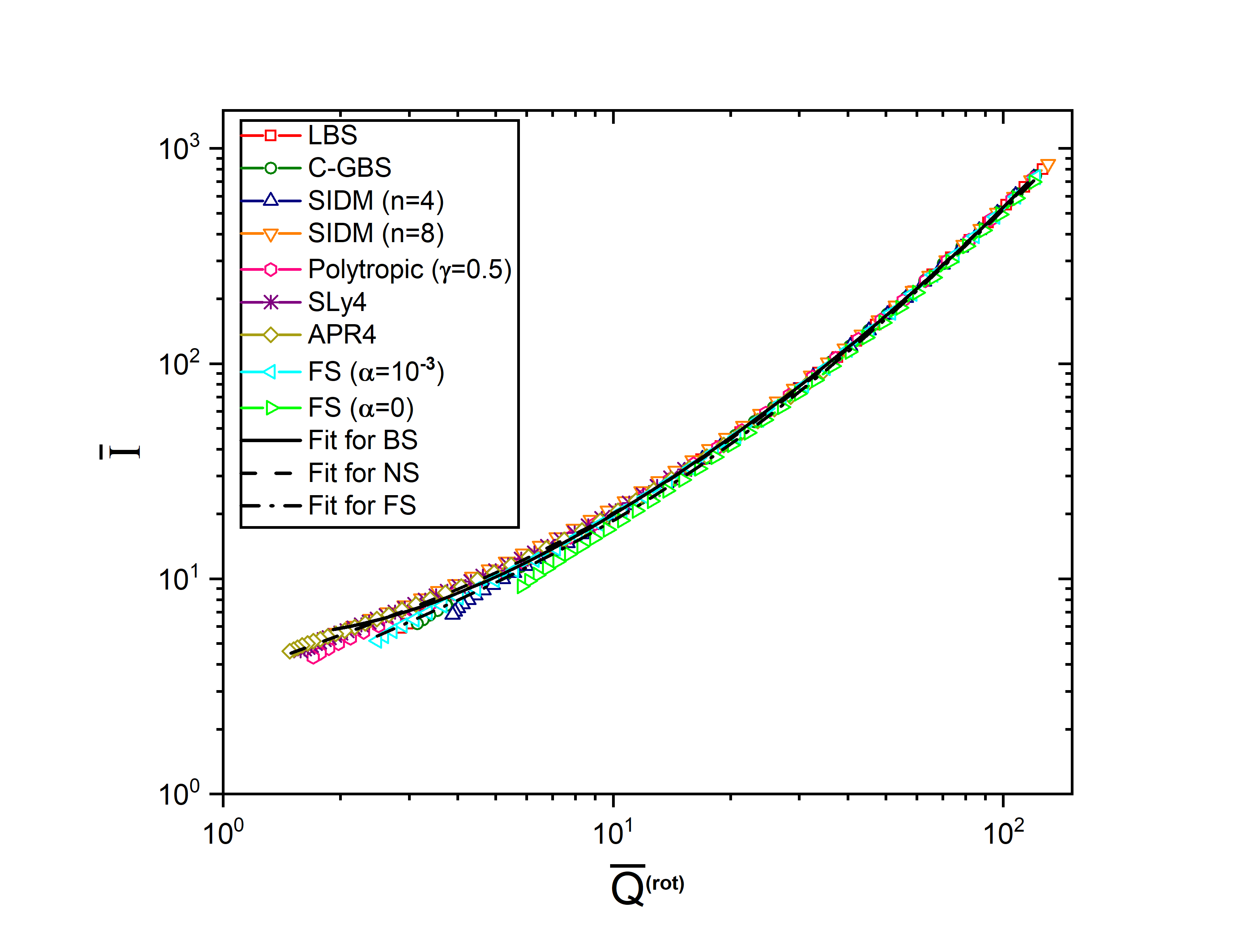
Figure 4: I-Q relations of 4 BS models, 2 FS models and 3 NS models. The meanings of different lines are the same as those in Fig.2.

$y_{i}$	$x_{i}$	$a_{i}$	$b_{i}$	$c_{i}$	$d_{i}$	$e_{i}$
$\bar{I}$	$\bar{\lambda}^{(tid)}$	1.74	-8.80$\times 10^{-2}$	4.74$\times 10^{-2}$	-2.33 $\times 10^{-3}$	4.52$\times 10^{-5}$
$\bar{I}$	$\bar{Q}^{(rot)}$	1.72	-0.217	0.462	-6.84$\times 10^{-2}$	5.40$\times 10^{-3}$
$\bar{Q}^{(rot)}$	$\bar{\lambda}^{(tid)}$	4.37$\times 10^{-2}$	0.268	7.50 $\times 10^{-3}$	-7.13 $\times 10^{-4}$	1.59$\times 10^{-5}$

Table 1: Numerical fitting for the I-Love, Q-Love and I-Q relations of the 4 BS models.

$y_{i}$	$x_{i}$	$a_{i}$	$b_{i}$	$c_{i}$	$d_{i}$	$e_{i}$
$\bar{I}$	$\bar{\lambda}^{(tid)}$	1.24	0.102	1.91$\times 10^{-2}$	-5.63 $\times 10^{-4}$	6.09$\times 10^{-6}$
$\bar{I}$	$\bar{Q}^{(rot)}$	0.898	1.01	-0.236	9.72$\times 10^{-2}$	-8.44$\times 10^{-3}$
$\bar{Q}^{(rot)}$	$\bar{\lambda}^{(tid)}$	0.131	0.232	1.37$\times 10^{-2}$	-1.16 $\times 10^{-3}$	2.70$\times 10^{-5}$

Table 2: Numerical fitting for the I-Love, Q-Love and I-Q relations of the 2 FS models.

$y_{i}$	$x_{i}$	$a_{i}$	$b_{i}$	$c_{i}$	$d_{i}$	$e_{i}$
$\bar{I}$	$\bar{\lambda}^{(tid)}$	1.41	7.62$\times 10^{-2}$	1.95$\times 10^{-2}$	-4.78 $\times 10^{-4}$	2.84$\times 10^{-6}$
$\bar{I}$	$\bar{Q}^{(rot)}$	1.23	0.715	-9.26$\times 10^{-2}$	6.29$\times 10^{-2}$	-5.39$\times 10^{-3}$
$\bar{Q}^{(rot)}$	$\bar{\lambda}^{(tid)}$	0.221	0.143	2.90$\times 10^{-2}$	-2.13 $\times 10^{-3}$	4.79$\times 10^{-5}$

Table 3: Numerical fitting for the I-Love, Q-Love and I-Q relations of the 3 NS models.

III I-Love-Q relations

With the techniques introduced in the appendix, we can calculate the moments of inertia $\bar{I}$, TLN $\bar{\lambda}^{(tid)}$ and quadrupole moments $\bar{Q}^{(rot)}$ for DS, along with those for NS serving as references. Fig.2, Fig.3 and Fig.4 show the I-Love, Q-Love and I-Q relations of these models, respectively. In addition, we make fittings for BS, FS and NS, with their I-Love-Q trios fitted on a log-log scale in a form as in Yagi:2013bca :

$$\ln y_{i}=a_{i}+b_{i}\ln x_{i}+c_{i}(\ln x_{i})^{2}+d_{i}(\ln x_{i})^{3}+e_{i}(\ln x_{i})^{4}.$$ (6)

In Table 1, 2 and 3, we list $a_{i}$, $b_{i}$, $c_{i}$, $d_{i}$ and $e_{i}$ for BS, FS and NS models, which respectively referred to the black solid line, dash-dot line and dashed line in Fig.[2, 3, 4].

We find that, the original I-Love-Q relation also apply to BS and FS, with some slight deviation when $\bar{\lambda}^{(tid)}<200$ (equivalently $\bar{I}<10$ or $\bar{Q}<4$). One interpretation for this phenomenon is that, those three parameters are mainly affected by the outer core of the compact stars, where the pressure and density are low. And all those DS EoS reduce to similar polytropic ones with $\gamma\leq 0.6$ when $p\to 0$. On the other hand, for small TLN, the stars are more compact and smaller in size, and the pressure is higher, and different EoS have different forms, which leads to more distinctions.

While the original relation is fitted up to approximately $\bar{\lambda}^{(tid)}=2\times 10^{4}$, the upper range for NS, here the upper range is set to $10^{8}$ like in PhysRevD.96.023005 , as DS might have larger TLN. We must emphasize that, if one compare with the original fitting table in Yagi:2013bca , the DS curves start deviating from the original I-Love-Q relation when $\bar{\lambda}^{(tid)}>10^{5}$. However, this merely arise from the fact that, the original curve is fitted to a smaller range, so the extension to high TLN will naturally not be accurate. In fact, when we fit the NS EoS up to $\bar{\lambda}^{(tid)}=10^{8}$, they coincide with the BS and FS curves at large TLN range. Actually, the whole I-Love-Q relations could be approximated by a single polytropic EoS with $\gamma=\frac{1}{2}$.

IV Conclusions

The moment of inertia, tidal Love number and quadrupole moment are insensitive to NS EoS, as proposed by Yagi and Yunes in Yagi:2013bca . In order to explore the properties of DS, we fit the I-Love-Q trio for four BS models, two FS models together with three NS models. It turns out that even for DS, the I-Love-Q relations still hold, with some small deviations when the star compactness is very large. The range of the original relation is expanded, and show high consistence within different models as the TLN grows (or equivalently the compactness falls).

Acknowledgements. The authors thank Feng-Li Lin and Zhoujian Cao for helpful discussions. KZ (Hong Zhang) is supported by a classified fund from Shanghai city.

Appendix A Solutions to Einstein Equation for Slowly-Rotating Compact Stars

In this appendix we review the basic construction, following Yagi:2013awa . Under a GR framework, the spacetime around a rotating compact star is described by the metric with Boyer-Lindqusit coordinates

$$\begin{split}&\mathrm{d}s^{2}=-e^{\nu(r)}[1+2\epsilon^{2}H_{2}(r)A_{2m}P_{2}^{m}(\cos\theta)]\mathrm{d}t^{2}\\ &+e^{\lambda(r)}[1+\frac{2\epsilon^{2}D_{2}(r)A_{2m}P_{2}^{m}(\cos\theta)}{r-m(r)}]\mathrm{d}r^{2}\\ &+r^{2}[1+2\epsilon^{2}K_{2}(r)A_{2m}P_{2}^{m}(\cos\theta)]\\ &\times\{\mathrm{d}\theta^{2}+\sin^{2}\theta[d\phi-\epsilon(\Omega-\omega_{1}(r)P^{\prime}_{1}(\cos\theta))\mathrm{d}t]^{2}\}+\mathcal{O}(\epsilon^{3}),\end{split}$$ (7)

where $A_{2m}=(-1)^{m}\frac{e^{im\phi}}{\sqrt{2\pi}}\sqrt{\frac{5(2-m)!}{2(2+m)!}}$, $P_{2}^{m}(\cos\theta)$ is the $[2,m]$ order associated Legendre polynomial and $P^{\prime}_{1}(\cos\theta)\equiv\frac{\mathrm{d}P_{1}(\cos\theta)}{\mathrm{d}\cos\theta}$ is the derivative of the 1st order Legendre polynomial. $\Omega$ represents the angular velocity. $m(r)$ is the mass of star within radius $r$ and $\lambda(r)\equiv-\ln(1-\frac{2m(r)}{r})$. $\epsilon$ is a parameter represents the order of expansion of perturbation on rotation. At the first order $\mathcal{O}(\epsilon)$, $\omega_{1}(r)$ denotes the rotation of NS 1967ApJ…150.1005H . At the second order $\mathcal{O}(\epsilon^{2})$, rotation of NS is introduced by $H_{2}(r),D_{2}(r)$ and $K_{2}(r)$. As stated in Yagi:2013awa , only spin and tidal deformations are considered that only $[l,m]=[0,0]$ and $[l,m]=[2,0]$ survive. Hence we keep $l=2$ modes and all $m$ orders.

According to Hartle 1967ApJ…150.1005H , when choosing a coordinate $(t,r,\theta,\phi)$ in perturbative questions, we should determine whether the perturbation is valid. For this model, the treatment is violated in the region where perturbed stars are almost the same order even the larger order than the unperturbed ones. To keep the perturbation valid, the radial coordinate should be transformed via

$$\bar{r}(r,\theta)=r+\epsilon^{2}\xi_{2}(r)A_{2m}P_{2}^{m}(\cos\theta)+\mathcal{O}(\epsilon^{3}),$$ (8)

where $\xi_{2}(r)$ has the effect that

$$\begin{split}\rho(\bar{r})=\rho(r)=\rho^{(0)}(r),\\ p(\bar{r})=p(r)=p^{(0)}(r).\end{split}$$ (9)

Here $\rho^{(0)}(r)$ and $p^{(0)}(r)$ mean the unperturbed density and pressure. Furthermore, other coefficients in Eq.(7) obey the same transformation. It is worth noting that $\xi_{2}(r)A_{2m}P_{2}^{m}(\cos\theta)$ is only well-defined inside the star, so we keep the exterior metric as the original one, as pointed out in Yagi:2013awa .

Since we have defined the spacetime of slow-rotation compact stars, the matter distribution is required to solve the Einstein equation. Considering the structure of stars as the perfect fluid, the energy-momentum tensor is defined by

$$T_{\mu\nu}=(\rho+p)u^{\mu}u^{\nu}+pg_{\mu\nu},$$ (10)

where $u^{\mu}=(u^{0},0,0,\epsilon\Omega u^{0})$.

The Einstein equation is solved analytically to construct a perturbed rotating star model with conditions introduced above. We obtain the structure from $(1)$ non-rotating terms, $(2)$ linear order terms in spin and $(3)$ quadratic order terms in spin. Matching with boundary solutions, the total mass, radius, moment of inertia, quadrupole moment and tidal deformation can be derived.

A.1 Non-rotating terms at $\mathcal{O}(\epsilon^{0})$

The interior configuration of stars can be described by unperturbed background solutions, which means that $m(r),\nu(r)$ and $\rho(r)$ satisfy the Tolman-Oppenheimer-Volkoff (TOV) equations 1992Advanced

$$\frac{\mathrm{d}m(r)}{\mathrm{d}r}=4\pi r^{2}\rho,$$ (11)

$$\frac{\mathrm{d}\nu(r)}{\mathrm{d}r}=\frac{2(4\pi r^{3}p+m)}{r(r-2m)},$$ (12)

$$\frac{\mathrm{d}p(r)}{\mathrm{d}r}=-\frac{(\rho+p)}{2}\frac{\mathrm{d}\nu}{\mathrm{d}r}.$$ (13)

In this paper, we rescale $m(r)$ by the mass of sun $M_{\odot}$ with other parameters by related astrophysical units:

$$r_{\odot}=\frac{G_{N}M_{\odot}}{c^{2}},\quad\rho_{\odot}=\frac{M_{\odot}}{r_{\odot}^{3}},\quad p_{\odot}=\frac{G_{N}M_{\odot}^{2}}{r_{\odot}^{4}},$$ (14)

where $G_{N}$ is the gravitational constant and $c$ is the speed of light. At the surface of stars, exterior solutions can be obtained by1967ApJ…150.1005H

$$\rho(R_{*})=p(R_{*})=0,$$ (15)

$$m(R_{*})=M_{*},$$ (16)

$$\nu(R_{*})=-\lambda(R_{*})=\ln(1-\frac{2M_{*}}{R_{*}}),$$ (17)

where $R_{*}$ is the total radius of a star. On the other hand, initial conditions are required to solve Equations (11) to (13). Staring from a infinitesimal core radius $r_{c}$, $m(r),\rho(r)$ and $p(r)$ are given by $\rho(r_{c})=\rho_{c},$ $p(r_{c})=p_{c},$ and $m(r_{c})=\frac{4\pi}{3}r_{c}^{3}\rho_{c}$.

A.2 Linear order terms at $\mathcal{O}(\epsilon^{1})$

In this section, we consider axisymmetric perturbations that only $(t,\phi)$ component of Einstein equations survives and $\omega_{1}(r)$ satisfy the equation Yagi:2013awa

$$\frac{\mathrm{d^{2}}\omega_{1}}{\mathrm{d}r^{2}}+\frac{4[1-\pi r^{2}(\rho+p)e^{\lambda}]}{r}\frac{\mathrm{d}\omega_{1}}{\mathrm{d}r}-16\pi r^{2}(\rho+p)e^{\lambda}\omega_{1}=0.$$ (18)

Outside of the stars, Eq.(18) is solved with conditions $\rho=p=0$ and the exterior solution has the form1967ApJ…150.1005H :

$$\omega^{ext}_{1}(r)=\Omega-\frac{2S}{r^{3}}=\Omega(1-\frac{2I}{r^{3}}),$$ (19)

where $S$ is the spin angular momentum and the moment of inertia $I$ is defined by $I\equiv\frac{S}{\Omega}.$

On the other hand, $I$ has a relationship with the interior solution $\omega_{1}^{int}$ 1967ApJ…150.1005H ; PhysRevD.61.024009

$$I=\frac{8\pi}{3\Omega}\int_{0}^{R_{*}}\frac{e^{-(\nu+\lambda)/2}r^{5}(\rho+p)\omega_{1}^{int}}{r-2m}\mathrm{d}r.$$ (20)

For the interior solution, Eq.(18) can be solved through numerical treatments with initial conditions. One can expand Eq.(18) at the center of stars to get the initial condition:Yagi:2013awa

$$\omega_{1}^{int}(r_{c})=\omega_{c}+\frac{8\pi}{5}(\rho_{c}+p_{c})\omega_{c}r_{c}^{2}+\mathcal{O}(r_{c}^{3}),$$ (21)

where $\omega_{c}$ is a constant remaining to be determined by matching the interior solution with the exterior one and their first derivatives at the surface of stars:

$$\omega_{1}^{int}(R_{*})=\omega_{1}^{ext}(R_{*}),\quad\omega_{1}^{\prime\,int}(R_{*})=\omega_{1}^{\prime\,ext}(R_{*}).$$ (22)

In solving Eq.(18) with these conditions, we find that $\omega_{1}$ is in direct proportion to $\Omega$, which means we can rescale $\omega_{1}$ by $\bar{\omega}_{c}=\omega_{c}/\Omega$. Hence for the interior and exterior solutions that $\bar{\omega}_{1}^{int}=\omega_{1}^{int}/\Omega$ and $\bar{\omega}_{1}^{ext}=\omega_{1}^{ext}/\Omega$. Once $\Omega$ is eliminated in Eq.(19), the exterior solution is completely determined by $I$, which depends on $\omega_{1}^{int}$, thus it is calculated by $\omega_{C}$. So we can set an arbitrary value to obtain $I$ and $\omega_{1}^{ext}$ and divide them by $\omega_{1}^{int}+\frac{2I}{R_{*}^{3}}$ to match the first boundary condition in Eq.(22) which is a convenient treatment in setting initial conditions. As stated in Yagi:2013awa , the dimensionless moment of inertia is introduced for subsequent convenient analysis, $\bar{I}=\frac{I}{M_{*}^{3}}$. From the above definition we can see that $\bar{I}\propto C^{-3}$, where $C\equiv\frac{M_{*}}{R_{*}}$ is the compactness of stars. For a BH, $\bar{I}\to 4$ while $C\to 0.5$Yagi:2013awa .

A.3 Quadratic order terms at $\mathcal{O}(\epsilon^{2})$

It can be seen in Eq.(7) that quadratic order terms in spin are described with $H_{2}(r),D_{2}(r)$ and $K_{2}(r)$. In solving Einstein Equations, we derive a differential equation of $D_{2}(r)$ from $(\theta,\theta)-(\phi,\phi)$ component, $H_{2}(r)$ from $(r,r)$ component and $K_{2}(r)$ from $(r,\theta)$ component. Eliminating the $D_{2}(r)$ terms in the formula of $H_{2}(r),K_{2}(r)$, we obtain 1967ApJ…150.1005H ; Yagi:2013awa ; PhysRevD.105.104018

$$\begin{split}\frac{\mathrm{d}K_{2}}{\mathrm{d}r}=&\frac{r^{2}}{8\pi r^{3}p+2m}[\frac{4m}{r^{3}}-8\pi(\rho+p)]H_{2}+\frac{2(H_{2}+K_{2})}{4\pi r^{3}p+m}\\ &+(1+\frac{r}{8\pi r^{3}p+2m})r^{3}e^{-\nu-\lambda}(\frac{\mathrm{d}\omega_{1}}{\mathrm{d}r})^{2}\\ &+(1-\frac{r}{8\pi r^{3}p+2m})e^{-\nu}\times 8\pi r^{3}(\rho+p)\omega_{1}^{2},\end{split}$$ (23)

$$\begin{split}\frac{\mathrm{d}H_{2}}{\mathrm{d}r}=&\{-\frac{8\pi r^{3}p+2m}{r(r-2m)}+\frac{r^{2}}{8\pi r^{3}p+2m}[8\pi(\rho+p)-\frac{4m}{r^{3}}]\}H_{2}\\ &-\frac{2(H_{2}+K_{2})}{4\pi r^{3}p+m}\\ &+(\frac{4\pi r^{3}p+m}{r-2m}-\frac{r}{8\pi r^{3}p+2m})r^{3}e^{-\nu-\lambda}(\frac{\mathrm{d}\omega_{1}}{\mathrm{d}r})^{2}\\ &+(\frac{4\pi r^{3}p+m}{r-2m}+\frac{r}{8\pi r^{3}p+2m})e^{-\nu}\times 8\pi r^{3}(\rho+p)\omega_{1}^{2}.\end{split}$$ (24)

The exterior solutions can be derived by considering the flatness at infinity, and at the boundary we have 1967ApJ…150.1005H ; Yagi:2013awa

$$\begin{split}K_{2}^{ext}(R_{*})=&-\frac{S^{2}}{M_{*}R_{*}^{3}}(1+2C)+\frac{3A}{C}[1+C-\frac{2}{3}C^{2}\\ &+\frac{(1-2C^{2})\ln(1-2C)}{2C}],\end{split}$$ (25)

$$\begin{split}H_{2}^{ext}(R_{*})=&\frac{S^{2}}{M_{*}R_{*}^{3}}(1+C)-\frac{3A}{C(1-2C)}[1-3C+\frac{4}{3}C^{2}\\ &+\frac{2}{3}C^{3}+\frac{(1-2C^{2})\ln(1-2C)}{2C}].\end{split}$$ (26)

Within a small core radius $r_{c}$, the interior solutions are acquired via Taylor-expanding Eq.(23, 24) 1967ApJ…150.1005H ; Yagi:2013awa ,

$$K_{2}^{int}(r_{c})=-Br_{c}^{2}+\mathcal{O}(r_{c}^{4}),$$ (27)

$$H_{2}^{int}(r_{c})=Br_{c}^{2}+\mathcal{O}(r_{c}^{4}).$$ (28)

In the above four equations, the constants $A$ and $B$ remain to be determined by boundary continuations,

$$K_{2}^{ext}(R_{*})=K_{2}^{int}(R_{*}),\quad H_{2}^{ext}(R_{*})=H_{2}^{int}(R_{*}).$$ (29)

Similarly to $\bar{I}$, we can divide $A$, $B$, $K_{2}$ and $H_{2}$ by $S^{2}$, making this parameter vanish. However, $\omega_{1}$ has been divided by $\Omega$ in the above section while $S\equiv I\Omega$, so we should divide $\omega_{1}$ and $\frac{\mathrm{d}\omega_{1}}{\mathrm{d}r}$ by $I$ in solving Eq.(23,24) if we apply the previous numerical results. In practice, a convenient treatment to determine $A$ and $B$ is setting an arbitrary value for $B$ first. The interior solutions then can be solved and consist of particular terms and homogeneous ones. Due to the linear dependence on $B$ for $K_{2}$ and $H_{2}$, the homogeneous solutions will get $n$ times larger if $B$ get $n$ times larger. The boundary conditions can be written as two linear equations1967ApJ…150.1005H ; PhysRevD.105.104018

$$K_{2}^{int}=K_{2}^{p}+nK_{2}^{h}=K_{2}^{ext},$$ (30)

$$H_{2}^{int}=H_{2}^{p}+nH_{2}^{h}=H_{2}^{ext},$$ (31)

where superscripts "$p$" and "$h$" are referred to the particular solution and the homogeneous solution. Once $A$ has been determined, we can derive the rotationally-induced quadrupole momentYagi:2013awa

$$Q^{(rot)}=-\frac{S^{2}}{M_{*}}-\frac{8}{5}AM_{*}^{3}.$$ (32)

The superscript "rot" represents that $Q$ is induced by spin. We rescale $Q^{(rot)}$ with $S^{2}$ and introduce the dimensionless quadrupole momentYagi:2013awa

$$\bar{Q}^{(rot)}\equiv-\frac{Q^{(rot)}M_{*}}{S^{2}}=1+\frac{8}{5}AM_{*}^{4}.$$ (33)

For the BH limit when the compactness $C$ approaches 0.5, $\bar{Q}$ approaches 1Yagi:2013awa .

A.4 Tidal perturbations at $\mathcal{O}(\epsilon^{2})$

Stars will response with tidal deformations if there is an external quadrupolar field, as the case in binary systems. The tidal deformation is at $\mathcal{O}(\epsilon^{2})$ for the leading order; hence it can be described by Eq.(23), (24). Since it is enough to consider a non-rotating state, $\omega_{1}$ and $\mathrm{d}\omega_{1}/\mathrm{d}r$ vanish in these two equations. After eliminating $K_{2}$, it gives Hinderer_2009 ; Yagi:2013awa

$$\begin{split}&\frac{\mathrm{d^{2}}H_{2}(r)}{\mathrm{d}r^{2}}+[\frac{2}{r}+(\frac{2m}{r^{2}}+4\pi r(p-\rho))e^{\lambda}]\frac{\mathrm{d}H_{2}(r)}{\mathrm{d}r}\\ &-[\frac{6e^{\lambda}}{r^{2}}-4\pi e^{\lambda}(5\rho+9p+(\rho+p)\frac{\mathrm{d}\rho}{\mathrm{d}p})+(\frac{\mathrm{d}\nu}{\mathrm{d}r})^{2}]H_{2}(r)=0.\end{split}$$ (34)

At the center $r_{c}$, we have the initial condition Hinderer_2009

$$H_{2}(r_{c})=c_{0}r_{c}^{2}[1-\frac{2\pi}{7}(5\rho_{c}+9p_{c}+(\rho_{c}+p_{c})\frac{\mathrm{d}\rho}{\mathrm{d}p}|_{r_{c}})r_{c}^{2}+\mathcal{O}(r_{c}^{3})],$$ (35)

where $c_{0}$ is a constant which can be solved with boundary conditions. For simplicity in numerical calculation, one can set a parameter $y(r)\equiv\frac{rH^{\prime}(r)}{H(r)}$ Hinderer_2009 , to end up with a first order differential equation for $y(r)$ ,

$$\begin{split}&\frac{\mathrm{d}y}{\mathrm{d}r}+\frac{y(y+1)}{r}+ye^{\lambda}(\frac{2m}{r^{2}}+4\pi r(p-\rho))-\frac{6e^{\lambda}}{r}\\ &+4\pi e^{\lambda}(5\rho+9p+(\rho+p)\frac{\mathrm{d}\rho}{\mathrm{d}p})+r(\frac{\mathrm{d}\nu}{\mathrm{d}r})^{2}=0.\end{split}$$ (36)

In this way, the initial condition is written as $y(r_{c})=2$ as $r_{c}\to 0$. When solving the above equation, we set boundary conditions as the same ones introduced in calculating non-rotating terms that $\rho(R_{*})=p(R_{*})=0$.

With $y(R_{*})$ in hand, we can calculate the TLN $\lambda^{(tid)}$ defined through

$$Q^{(tid)}_{ij}\equiv-\lambda^{(tid)}\mathcal{E}_{ij},$$ (37)

where $Q^{(tid)}_{ij}$ Hansen1974Multipole is the responded quadrupole moment and $\mathcal{E}_{ij}$ Geroch1970Multipole is the external quadrupolar tidal field, and the superscript "tid" represents the tidal effect. We now define the dimensionless TLN Flanagan2008Constraining

$$\bar{\lambda}^{(tid)}\equiv\frac{\lambda^{(tid)}}{M_{*}^{5}}=\frac{2}{3}\frac{k_{2}}{C^{5}},$$ (38)

where $k_{2}$ is calculated by $y(R_{*})$ and compactness $C$ via Hinderer_2009

$$\begin{split}k_{2}=&\frac{8C^{5}}{5}(1-2C)^{2}[2+2C(y-1)-y]\times\{2C[6-3y\\ &+3C(5y-8)]+4C^{3}[13-11y+C(3y-2)\\ &+2C^{2}(1+y)]+3(1-2C)^{2}[2-y\\ &+2C(y-1)]\ln(1-2C)\}^{-1}.\end{split}$$ (39)

References

- [1] B. P. Abbott et al. Observation of Gravitational Waves from a Binary Black Hole Merger. Phys. Rev. Lett., 116(6):061102, 2016.
- [2] B.P. Abbott et al. GW170817: Observation of Gravitational Waves from a Binary Neutron Star Inspiral. Phys. Rev. Lett., 119(16):161101, 2017.
- [3] B.P. Abbott et al. Properties of the binary neutron star merger GW170817. Phys. Rev. X, 9(1):011001, 2019.
- [4] F. Douchin and P. Haensel. A unified equation of state of dense matter and neutron star structure. Astron. Astrophys., 380:151, 2001.
- [5] A. Akmal, V. R. Pandharipande, and D. G. Ravenhall. The Equation of state of nucleon matter and neutron star structure. Phys. Rev. C, 58:1804–1828, 1998.
- [6] A. Rosenhauer, E.F. Staubo, L.P. Csernai, T. Øvergård, and E. Østgaard. Neutron stars, hybrid stars and the equation of state. Nuclear Physics A, 540(3):630–645, 1992.
- [7] Kilar Zhang, Takayuki Hirayama, Ling-Wei Luo, and Feng-Li Lin. Compact Star of Holographic Nuclear Matter and GW170817. Phys. Lett. B, 801:135176, 2020.
- [8] Kent Yagi and Nicolas Yunes. I-Love-Q. Science, 341:365–368, 2013.
- [9] Kent Yagi and Nicolas Yunes. I-Love-Q Relations in Neutron Stars and their Applications to Astrophysics, Gravitational Waves and Fundamental Physics. Phys. Rev. D, 88(2):023009, 2013.
- [10] H. Bondi and F. Hoyle. On the mechanism of accretion by stars. Mon. Not. Roy. Astron. Soc., 104:273, 1944.
- [11] H. Bondi. On spherically symmetrical accretion. Mon. Not. Roy. Astron. Soc., 112:195, 1952.
- [12] Maximilian Ruffert. Hydrodynamical 3-D Bondi-Hoyle accretion. 1. Code validation, stationary accretor. Astrophys. J., 427:342, 1994.
- [13] Maximilian Ruffert and David Arnett. Hydrodynamical 3-D Bondi-Hoyle accretion. 2. Homogeneous medium, mach 3, gamma = 5/3. Astrophys. J., 427:351, 1994.
- [14] M. Colpi, S. L. Shapiro, and I. Wasserman. Boson Stars: Gravitational Equilibria of Selfinteracting Scalar Fields. Phys. Rev. Lett., 57:2485–2488, 1986.
- [15] Kilar Zhang and Feng-Li Lin. Constraint on hybrid stars with gravitational wave events. Universe, 6(12):231, 2020.
- [16] Kilar Zhang, Ling-Wei Luo, Jie-Shiun Tsao, Chian-Shu Chen, and Feng-Li Lin. Dark stars and gravitational waves: Topical review, 2023.
- [17] Chris Kouvaris and Niklas Grønlund Nielsen. Asymmetric Dark Matter Stars. Phys. Rev. D, 92(6):063526, 2015.
- [18] There are two other conventions often encountered: or .
- [19] Monica Colpi, Stuart L. Shapiro, and Ira Wasserman. Boson stars: Gravitational equilibria of self-interacting scalar fields. Phys. Rev. Lett., 57:2485–2488, Nov 1986.
- [20] Andrea Maselli, Pantelis Pnigouras, Niklas Grønlund Nielsen, Chris Kouvaris, and Kostas D. Kokkotas. Dark stars: Gravitational and electromagnetic observables. Phys. Rev. D, 96:023005, Jul 2017.
- [21] James B. Hartle. Slowly Rotating Relativistic Stars. I. Equations of Structure. Astrophysics. J, 150:1005, December 1967.
- [22] John M Stewart and Malcolm Maccallum. Advanced general relativity. Physics Today, 45(6):83–84, 1992.
- [23] Vassiliki Kalogera and Dimitrios Psaltis. Bounds on neutron-star moments of inertia and the evidence for general relativistic frame dragging. Phys. Rev. D, 61:024009, Dec 1999.
- [24] Piyabut Burikham, Sitthichai Pinkanjanarod, and Supakchai Ponglertsakul. Slowly rotating neutron star with holographic multiquark core: I-love-q relations. Phys. Rev. D, 105:104018, May 2022.
- [25] Tanja Hinderer. Erratum: “tidal love numbers of neutron stars” (2008, apj, 677, 1216). The Astrophysical Journal, 697(1):964, may 2009.
- [26] Hansen and O. R. Multipole moments of stationary space-times. Journal of Mathematical Physics, 15(1):46–52, 1974.
- [27] Geroch and Robert. Multipole moments. ii. curved space. Journal of Mathematical Physics, 11(8):2580–2588, 1970.
- [28] éanna é. Flanagan and Tanja Hinderer. Constraining neutron-star tidal love numbers with gravitational-wave detectors. Physical Review D, 77(2):021502, 2008.