Distributed formation control of end-effector of mixed planar fully- and under-actuated manipulators

Abstract

This paper addresses the problem of end-effector formation control for a mixed group of two-link manipulators moving in a horizontal plane that comprises of fully-actuated manipulators and underactuated manipulators with only the second joint being actuated (referred to as the passive-active (PA) manipulators). The problem is solved by extending the distributed end-effector formation controller for the fully-actuated manipulator to the PA manipulator moving in a horizontal plane by using its integrability. This paper presents stability analysis of the closed-loop systems under a given necessary condition, and we prove that the manipulators’ end-effector converge to the desired formation shape. The proposed method is validated by simulations.

I Introduction

RECENTLY, the distributed formation control for manipulators has attracted significant interests, which allows a group of industrial manipulators to collectively carry out a complex task. For example, Wu et al. [1] investigate the distributed end-effector formation control of fully-actuated manipulators (the number of whose inputs is equal to its degree-of-freedom). The results are based on the use of virtual springs between the edges of an infinitesimally rigid formation graph of end-effectors. However, when underactuated manipulators (which have fewer inputs than the degree-of-freedom [2, 3, 4, 5, 6]) are used for some of the agents, the results are no longer applicable. In this case, it remains an open problem whether a desired formation shape can be made attractive by distributed control laws.

Underactuated manipulators have a wide range of applications due to the cheap cost and simple structure. Furthermore, one can regard a fully-actuated manipulator as underactuated when some of its joint actuators are faulty. In this regards, the control of an underactuated manipulator has been a central research topic for the past decades, which is particularly challenging owing to the second-order nonholonomic constraints [7, 8].

In this paper, we study the distributed end-effector formation control for a group of two-link manipulators moving in a horizontal plane, whose motions are not affected by gravity. Different from the work in [1], we consider that some manipulators in the group only have a single actuator at the second joint. These manipulators are referred to as the passive-active (PA) manipulator (see Fig. 1), which is a typical planar underactuated manipulator.

In our main results, we tackle some new difficulties in controller design and stability analysis. Firstly, we extend the distributed end-effector formation control for a group of fully-actuated manipulators in [1] to the above-mentioned mixed group of manipulators. For the PA manipulator with zero initial joint velocity (or joint angular velocity), the authors in [2] demonstrate its integrability and show that it is holonomic. That means the end-effector of the PA manipulator (with zero initial joint velocity) actually moves in a (curved) line rather than in a plane, and the end-effector position depends entirely on its actuated joint position (or joint angle). Based on the integrability, Lai et al. [6] derive constraints on the joint position/velocity of the PA manipulator with zero initial joint velocity. For solving the distributed formation control of fully-actuated manipulators’ end-effector, Wu et al. [1] use the Jacobian matrix of the fully-actuated manipulator which is obtained by taking the partial derivative of its end-effector position with respect to its joint position. Inspired by the result in [1], we are able to obtain the Jacobian matrix of the PA manipulator (with zero initial joint velocity) without relying on the computation of the derivative due to the results in [2] and [6].

Secondly, we present a mild condition such that the proposed distributed end-effector formation control laws are admissible, and subsequently we conduct the stability analysis for the closed-loop systems. In [1], Wu et al. assume that the Jacobian matrix of every fully-actuated manipulator is full rank, however, this condition can not be fulfilled by the PA manipulator since its Jacobian matrix reduces to a column vector. For the PA manipulator with zero initial joint velocity, we find another equation to obtain a square augmented Jacobian matrix. Under the condition of all obtained augmented Jacobian matrices being invertible and all fully-actuated manipulators’ Jacobian matrix being full rank, we prove that all manipulators’ end-effector converge to the desired formation shape. Through a number of simulation results, we show that the presented condition is always satisfied and the proposed control laws are effective if the group of manipulators starts from a neighborhood of the desired and reachable formation shape.

The rest of this paper is organized as follows. We present the manipulator dynamics and kinematics in Section II. Section II also contains some preliminaries on the graph theory, standard distributed formation control, and main problem formulation. Section III presents the distributed end-effector formation control laws and the corresponding stability analysis. Sections IV and V give simulation and the conclusions respectively.

II Preliminaries and Problem Formulation

This paper concerns the distributed end-effector formation control for a group of $N>1$ two-link manipulators moving in the same horizontal $X-Y$ plane. Consider that $N_{1}\geq 1$ of these manipulators are fully-actuated, and the rest $N_{2}=N-N_{1}$ manipulators are underactuated with a single actuator at their second joint, which we refer to as the PA manipulators. The manipulators’ mechanical parameters are described in Table I.

Notation: For column vectors $x_{1}$, …, $x_{n}$, let $\operatorname{col}\left(x_{1},\ldots,x_{n}\right):=\left[x_{1}^{\mathrm{T}},\ldots,x_{n}^{\mathrm{T}}\right]^{\mathrm{T}}$ be the stacked column vector. Use a short-hand notation $\bar{B}:=B\otimes I_{2}$, where $I_{2}\in\mathbb{R}^{2\times 2}$ is the identity matrix and $\otimes$ denotes the Kronecker product.

II-A Manipulator Dynamics and Kinematics

TABLE I: The mechanical parameters of manipulator $i$.

Symbol ($j=1,2$)	Description
$m_{i,j}$	Mass of link $j$
$I_{i,j}$	Moment of inertia of link $j$ with
	respect to its center-of-mass (COM)
$L_{i,j}$	Length of link $j$
$l_{i,j}$	Distance between joint $j$
	and the COM of link $j$
$q_{i,j}$	Angle of joint $j$
$u_{i,j}$	Torque applied to joint $j$

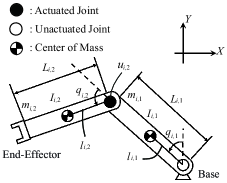
Figure 1: The PA manipulator: a planar two-link underactuated manipulator with an unactuated (or passive) first joint and an actuated (or active) second joint.

Based on the Euler-Lagrange equation [9, 10], the group of two-link planar manipulators is modeled by

$$M_{i}\left(q_{i}\right)\ddot{q}_{i}+C_{i}\left(q_{i},\dot{q}_{i}\right)\dot{q}_{i}=u_{i},$$ (1)

where $i\in\{1,...,N\}$, and $q_{i}=[q_{i,1},q_{i,2}]^{\mathrm{T}}$ is the generalized joint position. Without loss of generality, suppose that for all $i\in\{1,...,N_{1}\}$, the $i$-th manipulator is fully-actuated and $u_{i}=[u_{i,1},u_{i,2}]^{\mathrm{T}}$ is its generalized forces; otherwise for all $i\in\{N_{1}+1,...,N\}$, the $i$-th manipulator is an underactuated PA manipulator with $u_{i}=[0,u_{i,2}]^{\mathrm{T}}$. The matrix $M_{i}(q_{i})$ is the mass matrix and $C_{i}({q_{i}},{{\dot{q}}_{i}})$ is the Coriolis and centrifugal term, which are respectively given by

$$M_{i}\left(q_{i}\right) =\left[\begin{array}[]{lc}M_{i,11}\left(q_{i}\right)&M_{i,12}\left(q_{i}\right)\\ M_{i,21}\left(q_{i}\right)&M_{i,22}\left(q_{i}\right)\end{array}\right]$$

$$=\left[\begin{array}[]{cc}\alpha_{i,1}+\alpha_{i,2}+2\alpha_{i,3}\cos q_{i,2}&\alpha_{i,2}+\alpha_{i,3}\cos q_{i,2}\\ \alpha_{i,2}+\alpha_{i,3}\cos q_{i,2}&\alpha_{i,2}\end{array}\right],$$

$$C_{i}({q_{i}},{{\dot{q}}_{i}})={\alpha_{i,3}}\left[{\begin{array}[]{*{20}{c}}{-{{\dot{q}}_{i,2}}}&{-{{\dot{q}}_{i,1}}-{{\dot{q}}_{i,2}}}\\ {{{\dot{q}}_{i,1}}}&0\end{array}}\right]\sin{q_{i,2}},$$

where the mechanical parameters $\alpha_{i,1},\alpha_{i,2},\alpha_{i,3}$ are as follows

$$\left\{\begin{array}[]{l}\alpha_{i,1}=m_{i,1}l_{i,1}^{2}+m_{i,2}L_{i,1}^{2}+I_{i,1},\vspace{0.1cm}\\ \alpha_{i,2}=m_{i,2}l_{i,2}^{2}+I_{i,2},\vspace{0.1cm}\\ \alpha_{i,3}=m_{i,2}L_{i,1}l_{i,2}.\end{array}\right.$$ (2)

Property II.1

Following standard properties of Euler-Lagrange systems [10, 11], the manipulators (1) satisfy the following two properties:

1. The matrix $M_{i}(q_{i})$ is positive definite;

2. The matrix $\dot{M}_{i}(q_{i})-2C_{i}(q_{i},\dot{q}_{i})$ is skew-symmetric.

Accordingly, due to P1, we can rewrite (1) compactly as

$${\ddot{q}={M^{-1}}(q)\Big{(}\bar{u}-C(q,\dot{q})\dot{q}\Big{)}},$$ (3)

where $q=\operatorname{col}\left(q_{1},\ldots,q_{N}\right)\in\mathbb{R}^{2N}$, $\bar{u}=\operatorname{col}\left(u_{1},\ldots,u_{N}\right)\in\mathbb{R}^{2N}$ are the stacked vectors of $q_{i}$ and $u_{i}$ respectively and the matrices $M(q),C(q,\dot{q})\in\mathbb{R}^{2N\times 2N}$ are the block diagonal matrices of all $M_{i}(q_{i}),C_{i}(q_{i},\dot{q}_{i})$, respectively.

For manipulator $i$, let $x_{i}(t)\in\mathbb{R}^{2}$ be its end-effector position in the task-space, which can be obtained by

$$x_{i}:=[x_{i,X},x_{i,Y}]^{\mathrm{T}}=h_{i}\left(q_{i}\right)+x_{i0},\qquad$$ (4)

where $x_{i0}\in\mathbb{R}^{2}$ is the position of the fixed manipulator base and

$$h_{i}\left(q_{i}\right)=\left[{\begin{array}[]{*{20}{c}}{-{L_{i,1}}\sin\left({{q_{i,1}}}\right)-{L_{i,2}}\sin\left({{q_{i,1}}+{q_{i,2}}}\right)}\\ {{L_{i,1}}\cos\left({{q_{i,1}}}\right)+{L_{i,2}}\cos\left({{q_{i,1}}+{q_{i,2}}}\right)}\end{array}}\right].$$

Differentiating (4) with respect to time $t$ leads

$$\dot{x}_{i}=J_{i}\left(q_{i}\right)\dot{q}_{i},$$ (5)

$$J_{i}\left(q_{i}\right):=\frac{\partial h_{i}\left(q_{i}\right)}{\partial q_{i}}=\left[\begin{array}[]{ll}J_{i,11}\left(q_{i}\right)&J_{i,12}\left(q_{i}\right)\\ J_{i,21}\left(q_{i}\right)&J_{i,22}\left(q_{i}\right)\end{array}\right],$$

where $J_{i}(q_{i})$ is the Jacobian matrix [9, 10] of the manipulator $i$, and

$$J_{i,11}\left(q_{i}\right)=-L_{i,1}\cos\left(q_{i,1}\right)-L_{i,2}\cos\left(q_{i,1}+q_{i,2}\right),$$

$$J_{i,12}\left(q_{i}\right)=-L_{i,2}\cos\left(q_{i,1}+q_{i,2}\right),$$

$$J_{i,21}\left(q_{i}\right)=-L_{i,1}\sin\left(q_{i,1}\right)-L_{i,2}\sin\left(q_{i,1}+q_{i,2}\right),$$

$$J_{i,22}\left(q_{i}\right)=-L_{i,2}\sin\left(q_{i,1}+q_{i,2}\right).$$

II-B Properties of the Underactuated PA Manipulator

Let us recall some properties of the PA manipulator $i\in\{N_{1}+1,...,N\}$ given by (1) with $u_{i}=[0,u_{i,2}]^{\mathrm{T}}$. We denote $q_{i}(0)=[q_{i,1}(0),q_{i,2}(0)]^{\mathrm{T}}$ and $\dot{q}_{i}(0)=[\dot{q}_{i,1}(0),\dot{q}_{i,2}(0)]^{\mathrm{T}}$ as its initial joint position and initial joint velocity, respectively. Firstly, recall an important property on its joint position $q_{i}$ and joint velocity $\dot{q}_{i}$, which is presented by the following lemma and we refer to the results in [2, 6] for detailed discussion.

Lemma II.1

[2, 6] If the PA manipulator $i$ starts from a stationary position, i.e. $\dot{q}_{i}(0)=0$, then its joint velocity $\dot{q}_{i}$ satisfies

$$M_{i,11}(q_{i})\dot{q}_{i,1}+M_{i,12}(q_{i})\dot{q}_{i,2}=0.$$ (6)

Furthermore, assume that $q_{i,2}(0)\in[-\pi,\pi]$ and $q_{i,2}\in[-\pi+2k\pi,\pi+2k\pi]$, $k\in\mathbb{Z}$. Then the system is holonomic and its unactuated joint position $q_{i,1}$ depends entirely on its actuated joint position $q_{i,2}$ by

$${q_{i,1}}=f(q_{i,2})=-\frac{{{q_{i,2}}}}{2}-\gamma\arctan\left({\rho\tan\frac{{{q_{i,2}}}}{2}}\right)-\gamma k\pi+\eta,$$ (7)

where

$$\gamma=\frac{{{\alpha_{i,2}}-{\alpha_{i,1}}}}{{\sqrt{{{\left({{\alpha_{i,1}}+{\alpha_{i,2}}}\right)}^{2}}-4\alpha_{i,3}^{2}}}},\;\rho=\sqrt{\frac{{{\alpha_{i,1}}+{\alpha_{i,2}}-2{\alpha_{i,3}}}}{{{\alpha_{i,1}}+{\alpha_{i,2}}+2{\alpha_{i,3}}}}},$$

and $\displaystyle\eta=\frac{{{q_{i,2}}(0)}}{2}+{q_{i,1}}(0)+\gamma\arctan\left(\rho\tan\frac{{{q_{i,2}}(0)}}{2}\right)$.

Now, for the PA manipulator $i$, we rewrite (4) and (5) according to Lemma II.1. Substituting (7) into (4) gives us

$${x_{i}}:={\left[{{x_{i,X}},{x_{i,Y}}}\right]^{\rm{T}}}=\bar{h}_{i}\left({{q_{i,2}}}\right)+{x_{i0}},$$ (8)

where

$$\bar{h}_{i}\left(q_{i}\right)=\left[{\begin{array}[]{*{20}{c}}{-{L_{i,1}}\sin\left(f(q_{i,2})\right)-{L_{i,2}}\sin\left({f(q_{i,2})+{q_{i,2}}}\right)}\\ {{L_{i,1}}\cos\left(f(q_{i,2})\right)+{L_{i,2}}\cos\left({f(q_{i,2})+{q_{i,2}}}\right)}\end{array}}\right].$$

Note that $M_{i,11}(q_{i})>0$ due to $M_{i}(q_{i})$ being positive definite as in Property II.1. By using (6), we can rewrite (5) as

$$\dot{x}_{i} =\left[\begin{array}[]{ll}J_{i,11}\left(q_{i}\right)&J_{i,12}\left(q_{i}\right)\\ J_{i,21}\left(q_{i}\right)&J_{i,22}\left(q_{i}\right)\end{array}\right]\left[\begin{array}[]{l}\displaystyle\frac{-M_{i,12}\left(q_{i}\right)}{M_{i,11}\left(q_{i}\right)}\dot{q}_{i,2}\\ \dot{q}_{i,2}\end{array}\right]$$ (9)

$$=\bar{J}_{i}\left(q_{i}\right)\dot{q}_{i,2},$$

where the Jacobian matrix (vector) $\bar{J}_{i}\left(q_{i}\right)$ is

$$\bar{J}_{i}\left(q_{i}\right) =\left[\bar{J}_{i,1}\left(q_{i}\right),\bar{J}_{i,2}\left(q_{i}\right)\right]^{\mathrm{T}}$$

$$=\left[\begin{array}[]{c}\displaystyle-\frac{J_{i,11}\left(q_{i}\right)M_{i,12}\left(q_{i}\right)}{M_{i,11}\left(q_{i}\right)}+J_{i,12}\left(q_{i}\right)\vspace{0.1cm}\\ \displaystyle-\frac{J_{i,21}\left(q_{i}\right)M_{i,12}\left(q_{i}\right)}{M_{i,11}\left(q_{i}\right)}+J_{i,22}\left(q_{i}\right)\end{array}\right].$$

Note that we use the Jacobian matrix ${\bar{J}}_{i}(q_{i})$ in the distributed controller for the PA manipulator $i$. Two remarks on $\bar{J}_{i}(q_{i})$ are as follows.

Remark II.1

The Jacobian matrix ${\bar{J}}_{i}$ can be expressed as a function of $q_{i,2}$ only. When the real-time information of unactuated joint position $q_{i,1}$ is not available, we can instead use $q_{i,2}$ to substitute $q_{i,1}$ as given in (7). However, in this particular case, the distributed controller for the PA manipulator $i$ becomes complicated and is highly dependent on the initial joint position.

Remark II.2

We can also obtain the Jacobian matrix ${\bar{J}}_{i}$ by differentiating the end-effector position of the PA manipulator with respect to its actuated joint position similar to that for the fully-actuated manipulator, i.e. ${{\bar{J}}_{i}}=\frac{{\partial{\bar{h}_{i}}\left({{q_{i,2}}}\right)}}{{\partial{q_{i,2}}}}$. However, this approach is practically not feasible as it introduces computational complexity and makes the controller particularly complicated.

Define $\mathcal{W}_{i}$ as the working space of manipulator $i\in\{1,...,N\}$, and the entire working space for the networked manipulators is $\mathcal{W}:=\mathcal{W}_{1}\times\cdots\times\mathcal{W}_{N}$. According to (4), for the fully-actuated manipulator $i\in\{1,...,N_{1}\}$ modeled by (1) with $u_{i}=[u_{i,1},u_{i,2}]^{\mathrm{T}}$, we have

$$\mathcal{W}_{i}\subset\left\{x_{i}\in\mathbb{R}^{2}:x_{i}=h_{i}\left(q_{i}\right)+x_{i0},\;q_{i}\in\mathbb{R}^{2}\right\}.$$ (10)

Consider the PA manipulator $i\in\{N_{1}+1,...,N\}$ modeled by (1) with $u_{i}=[0,u_{i,2}]^{\mathrm{T}}$, which starts from $\dot{q}_{i}(0)=0$. Assume that $q_{i,2}(0)\in[-\pi,\pi]$ and $q_{i,2}\in[-\pi+2k\pi,\pi+2k\pi]$, $k\in\mathbb{Z}$. According to (8), we have

$$\mathcal{W}_{i}\subset\left\{x_{i}\in\mathbb{R}^{2}:x_{i}=\bar{h}_{i}\left(q_{i,2}\right)+x_{i0},\;q_{i,2}\in\mathbb{R}\right\}.$$ (11)

Note that, unlike the fully-actuated manipulator, the working space of the PA manipulator is in a line rather than a plane.

II-C Formation Graph and Mixed End-effector Distributed Formation Control Problem

For a given desired geometrical formation shape of manipulators’ end-effector, we can associate an undirected graph to the vertices and edges of the formation shape. Let us describe the corresponding formation graph by $\mathcal{G}:=\{\mathcal{V},\mathcal{E}\}$, where $\mathcal{V}:=\{1,\cdots,N\}$ is the vertex set and $\mathcal{E}\subset\mathcal{V}\times\mathcal{V}$ is the ordered edge set with $\mathcal{E}_{k}$ denoting the $k$-th edge. The numbers of vertices and edges of $\mathcal{G}$ are $|\mathcal{V}|=N$ and $|\mathcal{E}|$, respectively. The set of edges, where the end-effector $i$ is part of, is given by $\mathcal{I}_{i}:=\{k\in\{1,\ldots,|\mathcal{E}|\}:(i,j)=\mathcal{E}_{k}\text{ for some }j\}$. We define the elements of the incidence matrix $B\in\mathbb{R}^{N\times|\mathcal{E}|}$ of $\mathcal{G}$ by

$$b_{ik}=\left\{\begin{array}[]{ll}+1,&i=\mathcal{E}_{k}^{\text{tail }}\vspace{0.2cm}\\ -1,&i=\mathcal{E}_{k}^{\text{head }}\vspace{0.2cm}\\ 0,&\text{otherwise}\end{array}\;i=1,\ldots,N,\;k=1,\ldots,|\mathcal{E}|,\right.$$ (12)

where $\mathcal{E}_{k}^{\text{tail }}$ and $\mathcal{E}_{k}^{\text{head}}$ denote the tail and head nodes, respectively, of $\mathcal{E}_{k}$, i.e. $(\mathcal{E}_{k}^{\text{tail }},\mathcal{E}_{k}^{\text{head}})=\mathcal{E}_{k}$. Let us stack all end-effectors’ position $x_{i}$ into $x=\operatorname{col}\left(x_{1},\ldots,x_{N}\right)\in\mathbb{R}^{2N}$ and define the relative displacement $z$ by $z=\bar{B}^{\rm T}x$, whose elements correspond to the ordered $z_{k}:=x_{i}-x_{j}$. For a given desired formation shape defined by a vector of desired distances $d^{*}$ on the edges, let $x^{*}$ define a reference position such that $\|z_{k}(x^{*})\|=d_{k}^{*}$ for all $k\in\{1,...,|\mathcal{E}|\}$, where $d_{k}^{*}$ denotes the $k$-th element of $d^{*}$, i.e. the desired distance of the edge $\mathcal{E}_{k}$. Define the edge function $f_{\mathcal{G}}(x):=\mathop{\text{col}}\limits_{k\in\{1,\ldots,|\mathcal{E}|\}}\left(\|z_{k}\|^{2}\right)$, and the framework $(\mathcal{G},x^{*})$ is called infinitesimally rigid if the rank of $\frac{{\rm d}\hbox{\hskip 0.5pt}f_{\mathcal{G}}}{{\rm d}\hbox{\hskip 0.5pt}x}(x^{*})$ is $2N-3$ (for 2D shape). We refer interested readers to [12, 13, 14] and references therein for exposition on the rigid formation graph. Using the reference position $x^{*}$, let the set of all desired shapes be

$$\mathcal{S}:=\left\{x:x=\left(I_{N}\otimes R\right)x^{*}+\mathbf{1}_{N}\otimes b,R\in\mathbf{SO}(2),b\in\mathbb{R}^{2}\right\},$$ (13)

where $\mathbf{1}_{N}\in\mathbb{R}^{N}$ denotes the vector whose all elements are one. Let $\mathcal{S}_{W}:=\mathcal{S}\cap\mathcal{W}$ be the set of desired shapes that are also reachable by the networked manipulators.

Problem II.1

(Mixed Planar Fully-actuated and PA Manipulators’ End-Effector Distributed Formation Control Problem) For the above setup of networked two-link manipulators with mixed fully-actuated and PA manipulators and for a given desired infinitesimally rigid formation shape defined by the framework $(\mathcal{G},x^{*})$, design the distributed controller of the form

$$u_{i}=\sigma(\{z_{k}\}_{k\in\mathcal{I}_{i}},q_{i},\dot{q}_{i}),\;\;i=1,...,N,$$ (14)

such that $x(t)\to\mathcal{S}_{W}$ and $\dot{q}(t)\to 0$ as $t\to\infty$.

Note that due to the nature of the PA manipulators, the control inputs that are used for them are only those for the second joint. Hence for all $i\in\{N_{1}+1,\ldots,N\}$, the first element of $u_{i}$ is not used at all.

III Proposed Distributed Formation Controller

In the following, we will follow and modify accordingly the end-effector distributed formation controller presented in [1]. For a given desired distance vector $d^{*}$ associated to an infinitesimally rigid formation shape, we define the error $e_{k}\in\mathbb{R}$ on the edge $\mathcal{E}_{k}$ by $e_{k}:=\left\|z_{k}\right\|^{2}-(d_{k}^{*})^{2}$. Based on the error vector $e=\operatorname{col}(e_{1},\ldots,e_{|\mathcal{E}|})$, we define the potential function $V(e)$ for the formation by

$$V(e):=\frac{1}{2}\sum\limits_{k=1}^{\left|{\cal E}\right|}{e_{k}^{2}}.$$ (15)

In order to define the gradient-based distributed control for every manipulator $i\in\{1,...,N\}$, let $\hat{e}_{i}\in\mathbb{R}^{2}$ be the gradient of $V(e)$ along $x_{i}$, i.e. $\hat{e}_{i}:=\frac{\partial V(e)}{\partial x_{i}}$, which is expressed by the local relative displacement $z_{k}$ and the distance error $e_{k}$ for all $k\in\mathcal{I}_{i}$. Note that $\frac{{\partial{z_{k}}}}{{\partial{x_{i}}}}={b_{ik}}$ and let ${D_{k}}\left({{z_{k}}}\right):=\frac{{\partial{e_{k}}}}{{\partial{z_{k}}}}=2{z_{k}}$. Routine computation shows that

$${\hat{e}_{i}}=\sum\limits_{k=1}^{|{\cal E}|}{{b_{ik}}}{D_{k}}\left({{z_{k}}}\right){e_{k}}.$$ (16)

We can rewrite (16) in the following compact form

$$\hat{e}=\frac{\partial V(e)}{\partial x}=\bar{B}D(z)e,$$ (17)

where $\hat{e}=\operatorname{col}\left(\hat{e}_{1},\ldots,\hat{e}_{N}\right)\in\mathbb{R}^{2N}$ and the matrix $D(z)\in\mathbb{R}^{2|{\cal E}|\times|{\cal E}|}$ is the block diagonal matrix of $D_{k}(z_{k})$ for all $k\in\{1,\ldots,|\mathcal{E}|\}$. As discussed in [13], the matrix $D^{\mathrm{T}}(z)\bar{B}^{\mathrm{T}}\bar{B}D(z)$ is positive definite if $\mathcal{G}$ is infinitesimally and minimally rigid.

We are now ready to study the solvability of Problem II.1 and to present the distributed formation controller. Prior to that, we need the following assumptions.

Assumption 1

All PA manipulators start from a stationary position, i.e. $\dot{q}_{i}(0)=0$ for all $i\in\{N_{1}+1,\ldots,N\}$.

Let us briefly remark on this assumption. For the PA manipulator $i$, (6) is only satisfied under Assumption 1. When $\dot{q}_{i}(0)\neq 0$, we can not guarantee that the PA manipulator can be stabilized at a target position [6]. Assumption 1 is not restrictive since we can always make a manipulator start from a stationary position.

Assumption 2

There exists a neighborhood $\mathcal{S}_{W_{r}}$ of $\mathcal{S}_{W}$ s.t.

A1.

for every fully-actuated manipulator $i\in\{1,\ldots,N_{1}\}$, the Jacobian matrix $J_{i}(q_{i})$ as in (5) is full rank; and

A2.

for every PA manipulator $i\in\{N_{1}+1,\ldots,N\}$, the Jacobian matrix $\bar{J}_{i}(q_{i})$ as in (9) satisfies ${\bar{J}_{i,1}}(q_{i}){\bar{J}_{i,2}}(q_{i})\neq 0$

for all $x\in\mathcal{S}_{W_{r}}$.

Firstly, we note that for A1, the Jacobian matrix $J_{i}(q_{i})$ is not full rank only at $q_{i,2}=k\pi$ ($k\in\mathbb{Z}$) [10, p. 21]. Secondly, for the fulfillment of A2, the equation $\bar{J}_{i,1}(q_{i})\bar{J}_{i,2}(q_{i})=0$ only holds at some isolated points, which can be calculated numerically as we show later in the simulation. Assumption 2 is satisfied by continuity argument when the desired shape has been chosen at a reference point $x^{*}$ where $q_{i}=q_{i}^{*}$ for all $i\in\{1,...,N\}$, such that $J_{i}(q_{i}^{*})$ is full rank (for all $i\in\{1,...,N_{1}\}$) and $\bar{J}_{i,1}(q_{i}^{*})\bar{J}_{i,2}(q_{i}^{*})\neq 0$ (for all $i\in\{N_{1}+1,...,N\}$) in $\mathcal{S}_{W}$.

Theorem III.1

Consider the end-effector distributed formation control problem of mixed planar fully-actuated and PA manipulators in Problem II.1. Under Assumptions 1 and 2, the problem can be solved locally by distributed formation control laws

$$u_{i}=\left\{\begin{array}[]{rl}-{K_{P}}J_{i}^{\mathrm{T}}(q_{i}){\hat{e}_{i}}-{K_{D}}\dot{q}_{i},&i=1,...,N_{1},\\ &\\ \left[\begin{matrix}0\\ -K_{P}\bar{J}_{i}^{\mathrm{T}}(q_{i})\hat{e}_{i}-K_{D}\dot{q}_{i,2}\end{matrix}\right],&i=N_{1}+1,\ldots,N,\end{array}\right.$$ (18)

where $K_{P}>0$, $K_{D}>0$ are controller gains, the Jacobian matrices $J_{i}(q_{i})$, $\bar{J}_{i}(q_{i})$ and the vector ${\hat{e}_{i}}$ are as in (5), (9) and (16), respectively.

Proof:

Firstly, let us rewrite controllers (18) into the following compact form

$$u=-K_{P}J^{\mathrm{T}}(q)\hat{e}-K_{D}\xi,$$ (19)

$$J^{\mathrm{T}}(q)=\left[\begin{array}[]{cc}J_{\text{fa }}^{\mathrm{T}}\left(q_{\text{fa }}\right)&0\\ 0&\bar{J}_{\text{pa }}^{\mathrm{T}}\left(q_{\text{pa}}\right)\end{array}\right],$$

where “fa” and “pa” refer to the fully-actuated manipulators and the PA manipulators, respectively. The matrix $J_{\text{fa}}(q_{\text{fa}})\in\mathbb{R}^{{2N_{1}}\times{2N_{1}}}$ is the block diagonal matrix of $J_{i}(q_{i})$ for all $i\in\{1,...,N_{1}\}$ and $\bar{J}_{\text{pa}}(q_{\text{pa}})\in\mathbb{R}^{{2N_{2}}\times{N_{2}}}$ ($N_{2}=N-N_{1}$) is the block diagonal matrix of $\bar{J}_{i}(q_{i})$ for all $i\in\{N_{1}+1,...,N\}$. The stacked vectors $u,\xi,q_{\text{fa}},q_{\text{pa}}$ are respectively given by

$$u=\operatorname{col}\left(u_{1},\ldots,u_{N_{1}},u_{N_{1}+1,2},\ldots,u_{N,2}\right)\in\mathbb{R}^{2N_{1}+N_{2}},$$

$$\xi=\operatorname{col}\left(\dot{q}_{1},\ldots,\dot{q}_{N_{1}},\dot{q}_{N_{1}+1,2},\ldots,\dot{q}_{N,2}\right)\in\mathbb{R}^{2N_{1}+N_{2}},$$

$$q_{\text{fa}}=\operatorname{col}\left(q_{1},\ldots,q_{N_{1}}\right)\in\mathbb{R}^{2N_{1}},$$

$$q_{\text{pa}}=\operatorname{col}\left(q_{N_{1}+1},\ldots,q_{N}\right)\in\mathbb{R}^{2N_{2}}.$$

Consider the Lyapunov function as follows

$$U={K_{P}}V(e)+\frac{1}{2}{\dot{q}^{\mathrm{T}}}M(q){\dot{q}},$$ (20)

where $V(e)$ is as in (15). Routine computation to the time derivative of (20) yields

$$\dot{U} ={K_{P}}{\left({\frac{{\partial V}}{{\partial x}}}\right)^{\mathrm{T}}}\dot{x}+{{\dot{q}}^{\mathrm{T}}}(M(q)\ddot{q})+\frac{1}{2}{{\dot{q}}^{\mathrm{T}}}\dot{M}(q)\dot{q}$$

$$={K_{P}}{{\hat{e}}^{\mathrm{T}}}J(q)\xi+{{\dot{q}}^{\mathrm{T}}}(\bar{u}-C(q,\dot{q})\dot{q})+\frac{1}{2}{{\dot{q}}^{\mathrm{T}}}\dot{M}(q)\dot{q}$$

$$={K_{P}}{{\hat{e}}^{\mathrm{T}}}J(q)\xi+{{\dot{q}}^{\mathrm{T}}}\bar{u}={K_{P}}{{\hat{e}}^{\mathrm{T}}}J(q)\xi+{u^{\mathrm{T}}}\xi,$$ (21)

where the second equality is due to (17), (5), (9) and (3), and the third equality is due to P2 of Property II.1. Substituting (19) into (21) yields

$$\dot{U}=-{K_{D}}\|\xi\|^{2}.$$ (22)

It follows from the properness of $U$ and (22) that $e$, $\dot{q}$ are bounded and $\xi\in L^{2}({\mathbb{R}}_{+})$. Correspondingly, the boundedness of $e$ and $\dot{q}$ also implies that $\dot{\xi}\in L^{\infty}({\mathbb{R}}_{+})$, i.e. $\xi$ is uniformly continuous. By the generalized Barbalat’s lemma [15, Theorem 4.4], it implies that $\xi(t)\to 0$ as $t\to\infty$. Under Assumption 1 and using Lemma II.1, we have $\dot{q}(t)\to 0$ as $t\to\infty$, and consequently, from (3), $\bar{u}(t)\to 0$ as $t\to\infty$.

Accordingly, the asymptote of (19) satisfies

$$-{K_{P}}{J^{\mathrm{T}}(q)}\hat{e}=0.$$ (23)

Let us now decompose (23) into

$$-{K_{P}}J_{i}^{\mathrm{T}}(q_{i}){{\hat{e}}_{i}}=0,\quad i=1,...,N_{1},$$ (24)

and

$$-{K_{P}}\bar{J}_{i}^{\mathrm{T}}(q_{i}){{\hat{e}}_{i}}=0,\quad i=N_{1}+1,...,N.$$ (25)

On the one hand, under A1 in Assumption 2, $J_{i}(q_{i})$ is full rank in $S_{W_{r}}$, so that $\hat{e}_{i}=0$ for all $i\in\{1,...,N_{1}\}$ from (24). On the other hand, since $\bar{J}_{i}(q_{i})$ is not full rank, we need an additional equation to complete it. Note that for the PA manipulator $i$ with $\dot{q}_{i}(0)=0$, the end-effector position $x_{i}$ depends entirely on its actuated joint position $q_{i,2}$. Thus we have

$$\frac{{\partial V(e)}}{{\partial{q_{i,2}}}}=\frac{{\partial V(e)}}{{\partial{x_{i,X}}}}\frac{{\partial{x_{i,X}}}}{{\partial{q_{i,2}}}}=\frac{{\partial V(e)}}{{\partial{x_{i,Y}}}}\frac{{\partial{x_{i,Y}}}}{{\partial{q_{i,2}}}}.$$ (26)

Notice that ${{\hat{e}}_{i,1}}=\frac{{\partial V(e)}}{{\partial{x_{i,X}}}}$, ${{\hat{e}}_{i,2}}=\frac{{\partial V(e)}}{{\partial{x_{i,Y}}}}$, $\bar{J}_{i,1}(q_{i})=\frac{{\partial{x_{i,X}}}}{{\partial{q_{i,2}}}}$, $\bar{J}_{i,2}(q_{i})=\frac{{\partial{x_{i,Y}}}}{{\partial{q_{i,2}}}}$, so that we can rewrite (26) into

$${{\bar{J}}_{i,1}(q_{i})}{{\hat{e}}_{i,1}}-{{\bar{J}}_{i,2}(q_{i})}{{\hat{e}}_{i,2}}=0.$$ (27)

Combining (25) and (27) yields

$$\bar{J}_{i}^{*}(q_{i})\hat{e}_{i}=0,\;\bar{J}_{i}^{*}(q_{i}):=\left[\begin{array}[]{cc}\bar{J}_{i,1}(q_{i})&\bar{J}_{i,2}(q_{i})\\ \bar{J}_{i,1}(q_{i})&-\bar{J}_{i,2}(q_{i})\end{array}\right].$$ (28)

The matrix ${\bar{J}_{i}^{*}(q_{i})}$ is invertible if and only if ${\bar{J}_{i,1}}(q_{i}){\bar{J}_{i,2}}(q_{i})\neq 0$. Then, under A2 in Assumption 2, we have $\hat{e}_{i}=0$ for all $i\in\{N_{1}+1,...,N\}$ from (25). Therefore, we have $\hat{e}=0$. Since $D^{\mathrm{T}}(z)\bar{B}^{\mathrm{T}}$ is full rank, it follows immediately from (17) that in the asymptote we have $e=0$, i.e. $e(t)\to 0$ as $t\to\infty$. ∎

IV Simulation Results

We validate the distributed formation controller (18) by several numerical simulations in this section. We consider a network of $N=4$ two-link manipulators moving in the horizontal $X-Y$ plane. The mechanical parameters of these manipulators are the same as those in [1], where $m_{i,1}=1.2$ kg, $m_{i,2}=1.0$ kg, $l_{i,1}=l_{i,2}=0.75$ m, $L_{i,1}=L_{i,2}=1.5$ m, $I_{i,1}=0.2250\;\mathrm{kg}\mathrm{m^{2}}$ and $I_{i,2}=0.1875$ ${\mathrm{kg}}\mathrm{m^{2}}$ for $i=1,2,3,4$.

Let the desired formation shape be a square with side length of $0.4$ m. The incidence matrix $B$ of the corresponding formation graph $\mathcal{G}$ is

$$B=\left[\begin{array}[]{ccccc}1&0&0&-1&1\\ -1&1&0&0&0\\ 0&-1&1&0&-1\\ 0&0&-1&1&0\end{array}\right].$$

The manipulators’ base are fixed at $x_{10}=[0,0]^{\mathrm{T}}$, $x_{20}=[5,0]^{\mathrm{T}}$, $x_{30}=[5,3]^{\mathrm{T}}$ and $x_{40}=[0,3]^{\mathrm{T}}$, respectively. The manipulators start from $q_{1}(0)=[-\pi/2,\pi/3]^{\mathrm{T}}$, $q_{2}(0)=[\pi/6,\pi/3]^{\mathrm{T}}$, $q_{3}(0)=[\pi/2,\pi/3]^{\mathrm{T}}$ and $q_{4}(0)=[-\pi/2,-\pi/3]^{\mathrm{T}}$ with zero initial joint velocities, respectively. We use the distributed formation controller (18) with the controller gains of $K_{P}=800,K_{D}=600$. Correspondingly, we consider three numerical cases:

1. Case 1: Manipulators 1–3 are fully-actuated and manipulator 4 is the PA manipulator. The result is shown in Figs. 2–4.

2. Case 2: Manipulators 1 and 2 are fully-actuated, and manipulators 3 and 4 are the PA manipulators. The result is shown in Fig. 5.

3. Case 3: Manipulator 1 is fully-actuated and manipulators 2–4 are the PA manipulators. The result is shown in Fig. 6.

For Case 1, consider the Jacobian matrix $\bar{J}_{4}$ associated to the PA manipulator 4. As in Remark II.1, $\bar{J}_{4}$ can be expressed as a function of $q_{4,2}$ only. We can calculate numerically that $\bar{J}_{4,1}\bar{J}_{4,2}=0$ has only three solutions at $q_{4,2}=-1.3098,0.2137,2.2972$ for all $q_{4,2}\in(-\pi,\pi)$. That means Assumption 2 is satisfied if the manipulator 4 does not go through these three points and every manipulator $i\in\{1,2,3\}$ does not go through $q_{i,2}=k\pi,k\in\mathbb{Z}$. Fig. 2 shows the trajectories of the manipulators’ end-effector and Fig. 3 shows that the distances between the end-effectors converge to expected values. From Figs. 2 and 3, we observe that end-effectors in the network eventually form the expected formation shape. From Fig. 4, which shows all joint position and velocity signals, we notice that $-1.050<q_{4,2}<-1.005$ and $0.950<q_{i,2}<1.050$ ($i=1,2,3$). That means the manipulators do not go through the calculated singular points and Assumption 2 is satisfied.

Figs. 5 and 6 show that the distributed controller is also effective for Cases 2 and 3, including more underactuated PA manipulators in the network. Notice that the fully-actuated manipulators move in a 2D plane while the PA manipulators can only move in a line.

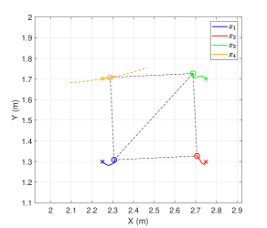
Figure 2: Simulation result of the distributed end-effector formation controller for Case 1. The colored solid lines are the trajectories of each manipulator’s end-effector, where $\times$ and $\circ$ denote initial positions and final positions respectively. The colored dashed line is the subset of the workspace of the PA manipulator.

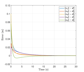
Figure 3: The plot of inter-agent distance error signals for the simulation of the distributed end-effector formation controller in Case 1.

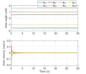
Figure 4: The plot of all joint position and velocity signals for the simulation of the distributed end-effector formation controller in Case 1.

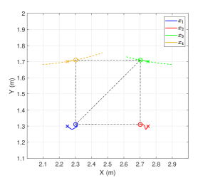
Figure 5: Simulation result of the distributed end-effector formation controller for Case 2. The colored solid lines are the trajectories of each manipulator’s end-effector, where $\times$ and $\circ$ denote initial positions and final positions respectively. The colored dashed lines are subsets of the workspace of each PA manipulator.

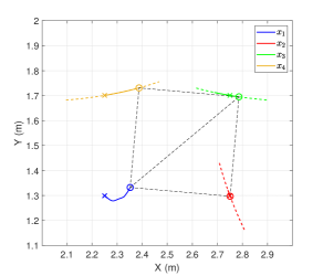
Figure 6: Simulation result of the distributed end-effector formation controller for Case 3. The colored solid lines are the trajectories of each manipulator’s end-effector, where $\times$ and $\circ$ denote initial positions and final positions respectively. The colored dashed lines are subsets of the workspace of each PA manipulator.

V Conclusion

This paper studied the end-effector distributed formation control for a mixed group of two-link manipulators moving in a horizontal plane, which comprises of fully-actuated manipulators and PA manipulators. Using the integrability property of the PA manipulator, we proposed and analyzed the distributed formation controller for end-effectors.

References

- [1] H. Wu, B. Jayawardhana, H. G. De Marina, and D. Xu, “Distributed formation control for manipulator end-effectors,” IEEE Transactions on Automatic Control, 2022, doi: 10.1109/TAC.2022.3225478.
- [2] G. Oriolo and Y. Nakamura, “Control of mechanical systems with second-order nonholonomic constraints: Underactuated manipulators,” in Proceedings of the 30th IEEE Conference on Decision and Control, vol. 3, 1991, pp. 2398–2403.
- [3] M. W. Spong, “The swing up control problem for the Acrobot,” IEEE Control Systems Magazine, vol. 15, no. 1, pp. 49–55, 1995.
- [4] I. Fantoni, R. Lozano, and M. W. Spong, “Energy based control of the Pendubot,” IEEE Transactions on Automatic Control, vol. 45, no. 4, pp. 725–729, 2000.
- [5] J. Wu, W. Ye, Y. Wang, and C. Su, “A general position control method for planar underactuated manipulators with second-order nonholonomic constraints,” IEEE Transactions on Cybernetics, vol. 51, no. 9, pp. 4733–4742, 2019.
- [6] X. Lai, J. She, W. Cao, and S. X. Yang, “Stabilization of underactuated planar Acrobot based on motion-state constraints,” International Journal of Non-Linear Mechanics, vol. 77, pp. 342–347, 2015.
- [7] I. Fantoni and R. Lozano, Non-linear control for underactuated mechanical systems. Springer, 2001.
- [8] X. Xin and Y. Liu, Control design and analysis for underactuated robotic systems. Springer, 2014.
- [9] R. M. Murray, Z. Li, and S. S. Sastry, A mathematical introduction to robotic manipulation. CRC press, 2017.
- [10] M. W. Spong, S. Hutchinson, and M. Vidyasagar, Robot modeling and control. John Wiley & Sons, 2020.
- [11] R. Ortega, A. Loría, P. J. Nicklasson, and H. Sira-Ramírez, Passivity-based control of Euler-Lagrange systems: mechanical, electrical and electromechanical applications. Springer Science & Business Media, 1998.
- [12] N. P. K. Chan, B. Jayawardhana, and H. G. de Marina, “Angle-constrained formation control for circular mobile robots,” IEEE Control Systems Letters, vol. 5, no. 1, pp. 109–114, 2021.
- [13] H. G. de Marina, “Distributed formation control for autonomous robots,” Ph.D. dissertation, University of Groningen, 2016.
- [14] H. G. de Marina, B. Jayawardhana, and M. Cao, “Taming mismatches in inter-agent distances for the formation-motion control of second-order agents,” IEEE Transactions on Automatic Control, vol. 63, no. 2, pp. 449–462, 2018.
- [15] H. Logemann and E. P. Ryan, “Asymptotic behaviour of nonlinear systems,” The American Mathematical Monthly, vol. 111, no. 10, pp. 864–889, 2004.