Improved Shortest Path Restoration Lemmas for Multiple Edge Failures: Trade-offs Between Fault-tolerance and Subpaths

Abstract

The restoration lemma is a classic result by Afek, Bremler-Barr, Kaplan, Cohen, and Merritt [PODC ’01], which relates the structure of shortest paths in a graph $G$ before and after some edges in the graph fail. Their work shows that, after one edge failure, any replacement shortest path avoiding this failing edge can be partitioned into two pre-failure shortest paths. More generally, this implies an additive tradeoff between fault tolerance and subpath count: for any $f,k$, we can partition any $f$-edge-failure replacement shortest path into $k+1$ subpaths which are each an $(f-k)$-edge-failure replacement shortest path. This generalized result has found applications in routing, graph algorithms, fault tolerant network design, and more.

Our main result improves this to a multiplicative tradeoff between fault tolerance and subpath count. We show that for all $f,k$, any $f$-edge-failure replacement path can be partitioned into $O(k)$ subpaths that are each an $(f/k)$-edge-failure replacement path. We also show an asymptotically matching lower bound. In particular, our results imply that the original restoration lemma is exactly tight in the case $k=1$, but can be significantly improved for larger $k$. We also show an extension of this result to weighted input graphs, and we give efficient algorithms that compute path decompositions satisfying our improved restoration lemmas.

1 Introduction

Suppose we want to route information, traffic, goods, or anything else along shortest paths in a distributed network. In practice, network edges can be prone to failures, in which a link is temporarily unusable as it awaits repair. It is therefore desirable for a system to be able to adapt to these failures, efficiently rerouting paths on the fly into new replacement shortest paths that avoid the currently-failing edges.

An algorithm that repairs a shortest path routing table following one or more edge failures is called a restoration algorithm [BBAK⁺01]. An ideal restoration algorithm will avoid recomputing shortest paths from scratch after each new failure event, instead leveraging its knowledge of the pre-failure shortest paths to speed up the computation of the post-failure replacement shortest paths. Therefore, when designing restoration algorithms, it is often helpful to understand exactly how shortest paths in a graph can evolve following edge failures. A restoration lemma is the general name for a structural result relating the form of pre-failure shortest paths to post-failure shortest paths in a graph, named for their applications in restoration algorithms.

The original restoration lemma was pioneered in a classic paper by Afek, Bremler-Barr, Kaplan, Cohen, and Meritt [BBAK⁺01]. All graphs in this discussion are undirected and unweighted, until otherwise indicated.

Definition 1 (Replacement Paths).

A path $\pi$ in a graph $G=(V,E)$ is an $f$-fault replacement path if there exists a set of edges $F\subseteq E,|F|\leq f$ such that $\pi$ is a shortest path in the graph $G\setminus F$.

Theorem 2 (Original Restoration Lemma [BBAK⁺01]).

In any graph $G$, every $f$-fault replacement path can be partitioned into $f+1$ subpaths that are each a shortest path in $G$.

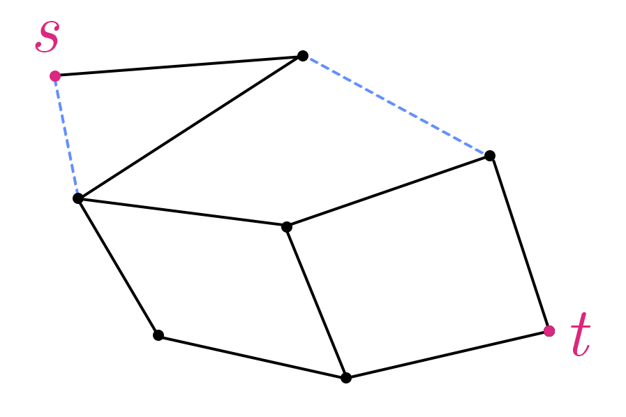
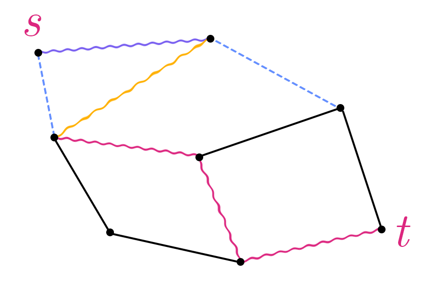
Figure 1: (Left) Suppose that two blue dashed edges in the graph fail. (Right) The restoration lemma guarantees that any shortest $s\leadsto t$ path (indicated with wavy edges) in the post-failure network can be partitioned into three subpaths, which are each a shortest path in the pre-failure network.

This restoration lemma suggests a natural approach for restoration algorithms: when $f$ edges fail and an $s\leadsto t$ shortest path is no longer usable, we can find a replacement $s\leadsto t$ shortest path by searching only over $s\leadsto t$ paths that can be formed by concatenating $f+1$ shortest paths that we have already computed in the current routing table. Up to some subtleties involving shortest path tiebreaking [BP21], this approach works, and has been experimentally validated as an efficient restoration strategy [BBAK⁺01]. It has also found widespread theoretical application, e.g. in pricing algorithms [HS01], replacement path algorithms [BP21, BCG⁺18, MMG89, CC19, GJM20], fault-tolerant variants of spanner problems [BP21, BGPW17, CCFK17], and more.

1.1 The Fault Tolerance/Subpath Count Tradeoff and First Main Result

Most applications of the restoration lemma in the previous literature are actually based on the following more general phrasing of Theorem 2:

Corollary 3 ([BBAK⁺01]).

For any graph $G$ and any $1\leq k\leq f$, every $f$-fault replacement path can be partitioned into $k+1$ subpaths that are each $(f-k)$-fault replacement paths in $G$.

In other words, there are two parameters of the decomposition that we might want to minimize: the number of subpaths in the decomposition, and the complexity of each subpath, as measured by the number of faults that would need to be excluded to make each subpath a shortest path. Theorem 2 is the special case $k=f$ of this corollary. Despite the apparent added generality of Corollary 3, it follow from Theorem 2 in a simple way:

Proof of Corollary 3, given Theorem 2.

Let $\pi$ be a replacement shortest path in a graph $G$ avoiding a set of edge failures $F=\{e_{1},\dots,e_{f}\}$. Consider the graph $G^{\prime}:=G\setminus\{e_{1},\dots,e_{f-k}\}$. In $G^{\prime}$, $\pi$ is a $k$-fault replacement shortest path avoiding the remaining edge failures $\{e_{f-k+1},\dots,e_{f}\}$. Thus, applying Theorem 2 in $G^{\prime}$, we can partition $\pi$ into $k+1$ subpaths that are each a shortest path in $G^{\prime}$. Each of these subpaths is thus an $(f-k)$-replacement shortest path, avoiding $\{e_{1},\dots,e_{f-k}\}$, in the original graph $G$. ∎

Corollary 3 promises an additive tradeoff between subpath count and fault tolerance of each subpath. However, it is not known whether this tradeoff is optimal. For example, we could optimistically hope for a multiplicative tradeoff between fault tolerance and subpath count: it is consistent with current knowledge that every $f$-fault replacement path could be partitioned into only two $f/2$-fault replacement paths, rather than the partition into $(f/2-1)$ many $f/2$-fault replacement paths promised by Corollary 3.

The main contribution of this work is to mostly settle the tradeoff between fault tolerance and subpath count available to restoration lemmas, up to a constant factor:

Theorem 4 (Main Result).

The following hold for all positive integers $k,f$ with $k\leq f$:

• (Upper Bound) In any graph $G$, every $f$-fault replacement path can be partitioned into $O(k)$ subpaths that are each an replacement path in $G$ avoiding at most $f/k$ faults.

• (Lower Bound) There are graphs $G$ and $f$-fault replacement paths $\pi$ that cannot be partitioned into $2k$ subpaths that are each an $(\lfloor f/k\rfloor-2)$-fault replacement path in $G$.

In our view, Theorem 4 contains both good news and bad news for the area. The good news is that the restoration lemma tradeoff is in fact multiplicative in nature, and so it can be substantially improved for most choices of $k$. This potentially opens up new avenues for improved restoration algorithms for routing table recovery, as explored by Afek et al. [BBAK⁺01]. The bad news is that, in the case $k=1$, our new lower bound shows that the previous restoration lemma was tight: there are examples in which one cannot decompose an $f$-fault replacement path into two replacement paths avoiding $f-2$ faults each. This case $k=1$ is particularly important in applications, especially to spanner and preserver problems [BP21, BGPW17], and so this lower bound may close a promising avenue for progress on these applications.

1.2 Weighted Restoration Lemmas and Second Main Result

The original paper by Afek et al. [BBAK⁺01] also proved a weighted restoration lemma, which gives a weaker decomposition, but which holds also for weighted input graphs:

Theorem 5 (Weighted Restoration Lemma [BBAK⁺01]).

For any weighted graph $G$ and any $1\leq k\leq f$, every $f$-fault replacement path $\pi$ can be partitioned into $k+1$ subpaths and $k$ individual edges, where each subpath in the partition is an $(f-k)$-fault replacement path in $G$.

More specifically, this theorem promises that the subpaths and individual edges occur in an alternating pattern (although some of these subpaths in this pattern may be empty). One can again ask whether this additive tradeoff between subpath count and fault tolerance per subpath is optimal. We show that it is not, and that it can be improved to a multiplicative tradeoff, similar to Theorem 4.

Theorem 6 (Main Result, Weighted Setting).

For any weighted graph $G$ and any $1\leq k\leq f$, every $f$-fault replacement path $\pi$ can be partitioned into $O(k)$ subpaths and $O(k)$ individual edges, where each subpath in the partition is an $(f/k)$-fault replacement path in $G$.

For most graphs of interest, this theorem can be simplified. For example, suppose we consider the setting of metric input graphs, in which every edge must be a shortest path between its endpoints. Then we can consider the $O(k)$ individual edges in the decomposition to be $0$-fault replacement paths, and so we could correctly state that $\pi$ can be partitioned into $O(k)$ subpaths that are each at most $(f/k)$-fault replacement paths. Every unweighted graph is a metric graph, and so in this sense our weighted main result generalizes our unweighted upper bound. However, we also note that our weighted main result cannot be simplified in general: one can easily construct weighted graphs containing edges $(u,v)$ that are $f$-fault replacement paths between their endpoints, but not $(f-1)$-fault replacement paths, and therefore any weighted restoration lemma will need to include some exceptional edges, as in [BBAK⁺01] and Theorem 6.

1.3 Algorithmic Considerations

In the main body of the paper, our restoration lemmas (both weighted and unweighted) are proved using a simple but slow greedy decomposition strategy to determine the subpaths; essentially, we repeatedly peel off the longest possible prefix from the input path $\pi$ that is an $f/k$-fault replacement path. All of our technical work is in proving a bound of $O(k)$ on the number of subpaths that arise from this decomposition. However, we note that this process requires exponential time in the number of faults $f$. That is, given a subpath $\pi_{i}\subseteq\pi$, we can straightforwardly test whether $\pi_{i}$ is an $f/k$-fault replacement path via brute force search over every subset of faults $F^{\prime}\subseteq F,|F^{\prime}|\leq f/k$. This requires $\text{poly}(n)\cdot\exp(f)$ time, and it is not clear if this $\exp(f)$ factor can be improved.

We thus revisit the decomposition strategy in Section 6, and show a more involved algorithm that implements our restoration lemmas in $\text{poly}(n,f)$ time. That is:

Theorem 7 (Unweighted Algorithmic Restoration Lemma).

There is an algorithm that take on input a graph $G$, a set $F$ of $|F|=f$ edge faults, a shortest path $\pi$ in $G\setminus F$, and a parameter $k$, and which returns:

• A partition $\pi=\pi_{0}\circ e_{0}\circ\pi_{1}\circ\dots\circ\pi_{q}$ into $q=O(k)$ subpaths, and

• Fault sets $F_{0},\dots,F_{q}\subseteq F$ with each $|F_{i}|\leq f/k$, such that each path $\pi_{i}$ in the decomposition is a shortest path in $G\setminus F_{i}$

(hence the algorithm implements Theorem 4). This algorithm runs in polynomial time in both the number of nodes $n$ and the number of faults $f$.

The core of of our new decomposition approach is a reduction to the algorithmic version of Hall’s theorem; this is somewhat involved, and so we overview it in more depth in the next part of this introduction. Using roughly the same algorithm, we also show the algorithmic restoration lemma in the weighted setting.

Theorem 8 (Weighted Algorithmic Restoration Lemma).

There is an algorithm that take on input a weighted graph $G$, a set $F$ of $|F|=f$ edge faults, a shortest path $\pi$ in $G\setminus F$, and a parameter $k$, and which returns:

• A partition $\pi=\pi_{0}\circ e_{0}\circ\dots\circ\pi_{q-1}\circ e_{q-1}\circ\pi_{q},$ where each $\pi_{i}$ is a (possibly empty) subpath, each $e_{i}$ is a single edge, and $q=O(k)$, and

• Fault sets $F_{0},\dots,F_{q}\subseteq F$ with each $|F_{i}|\leq f/k$, such that each path $\pi_{i}$ in the decomposition is a shortest path in $G\setminus F_{i}$

(hence the algorithm implements Theorem 6). This algorithm runs in polynomial time in both the number of nodes $n$ and the number of faults $f$.

1.4 Technical Overview of Upper Bounds

The more involved parts of the paper are the upper bound in Theorem 4, and Theorem 6. We will overview the proof in the unweighted setting (Theorem 4) here. The weighted setting carries a few additional details, but more or less follows the same proof strategy.

Let $\pi$ be an $f$-fault replacement path in an input graph $G$ with endpoints $(s,t)$; in particular, let $F$ be a set of $|F|\leq f$ edge faults, and suppose that $\pi$ is a shortest $s\leadsto t$ path in the graph $G\setminus F$. We are also given a parameter $f^{\prime}<f$, and our goal is to partition $\pi$ into as few subpaths as possible, subject to the constraint that each subpath is a replacement path avoiding at most $f^{\prime}$ faults.

The Partition of $\pi$.

We use a simple greedy process to determine the partition of $\pi$. We will determine a sequence of nodes $(s=x_{0},x_{1},\dots,x_{k},x_{k+1}=t)$ along $\pi$, which form the boundaries between subpaths in the decomposition. Start with $s=:x_{0}$, and given node $x_{i}$, define $x_{i+1}$ to be the furthest node following $x_{i}$ such that the subpath $\pi[x_{i},x_{i+1}]$ is an $f^{\prime}$-fault replacement path. We will denote the subpath $\pi[x_{i},x_{i+1}]$ as $\pi_{i}$, and so the decomposition is

$$\pi=\pi_{0}\circ\dots\circ\pi_{k}.$$

We will let $F_{i}\subseteq F,|F_{i}|\leq f^{\prime}$ be an edge set such that $\pi_{i}$ is a shortest $x_{i}\leadsto x_{i+1}$ path in the graph $G\setminus F_{i}$. Each subpath $i$ might allow several valid choices of fault set $F_{i}$; it will be important for our argument to define $F_{i}$ to be a fault set of minimum size $|F_{i}|$.

Our goal is now to show that the parameter $k$, defined as (one fewer than) the number of subpaths that arise from the greedy decomposition, satisfies $kf^{\prime}\leq O(f)$.

Argument Under Simplifying Assumptions.

Our proof strategy will be to prove that an arbitrary faulty edge $e\in F$ can appear in only a constant number of subpath fault sets $F_{i}$, which implies that $kf^{\prime}\leq O(f)$ by straightforward counting. To build intuition, let us see how the proof works under two rather strong simplifying assumptions:

• (Equal Subpath Assumption) We will assume that all subpaths in the decomposition have equal length: $|\pi_{0}|=\dots=|\pi_{k}|$.

• (First Fault Assumption) Let us say that a shortcut for a subpath $\pi_{i}$ is an alternate $x_{i}\leadsto x_{i+1}$ path in the original graph $G$ that is strictly shorter than $\pi_{i}$. Every shortcut must contain at least one fault in $F_{i}$, and conversely, every fault in $F_{i}$ lies on at least one shortcut (or else it may be dropped from $F_{i}$). Our second simplifying assumption is that, more specifically, for each $e\in F_{i}$ there exists a shortcut $\sigma$ for $\pi_{i}$ such that $e$ is the first fault in $F_{i}$ on $\sigma$.

Figure 2: Under the equal subpath and first fault assumptions, we can reach contradiction if we assume that there are three different subpaths that all have shortcuts that use $e$ as their first fault.

With these two assumptions in hand, we are ready to prove that each faulty edge $e$ appears in only $O(1)$ many fault sets $F_{i}$. Suppose for contradiction that there are three separate subpaths that all have shortcuts that use $e$ as their first edge, and moreover that these shortcuts use $e$ with the same orientation. Consider the first and last of these shortcut prefixes, which we will denote as $q(x_{1},u)$ and $q(x_{3},u)$. In Figure 2, the shortcuts are represented as dotted paths, and $q(x_{1},u),q(x_{3},u)$ are colored red. Notice that $q(x_{1},u)\cup q(x_{3},u)$ form an alternate $x_{1}\leadsto x_{3}$ path. Since $e$ is assumed to be the first fault on these shortcuts, this alternate $x_{1}\leadsto x_{3}$ path avoids all faults in $F$. Additionally, by definition of shortcuts we have

$$|q(x_{1},u)|+|q(x_{3},u)|<\left|\pi_{1}\right|+\left|\pi_{3}\right|.$$

Since we have assumed that all subpaths have the same length, we can amend this to

$$|q(x_{1},u)|+|q(x_{3},u)|<\left|\pi_{1}\right|+\left|\pi_{2}\right|.$$

But this implies that $q(x_{1},u)\cup q(x_{3},u)$ forms an $x_{1}\leadsto x_{3}$ path that is strictly shorter than the one used by $\pi$, which contradicts that $\pi$ is a shortest path in $G\setminus F$. This completes the simplified proof, but the challenge is now to relax our two simplifying assumptions, which are currently doing a lot of work in the argument.

Relaxing the Equal-Subpath-Length Assumption.

The equal-subpath-length assumption is the easier of the two to relax. It is only used in one place in the previous proof: to replace $|\pi_{3}|$ with $|\pi_{2}|$ in the inequality. When we drop the assumption, if we get lucky and have $|\pi_{2}|\geq|\pi_{3}|$, then the previous proof still works. The bad case is when $|\pi_{2}|<|\pi_{3}|$.

To handle this bad case, we follow a proof strategy from [ABDS⁺20]. Let us say that a subpath is pre-light if it is no longer than the preceding subpath, or post-light if it is no longer than the following subpath. In the above example, $\pi_{2}$ is pre-light if we have $|\pi_{2}|\leq|\pi_{1}|$, and it is post-light if $|\pi_{2}|\leq|\pi_{3}|$. It is possible for a particular subpath to be both pre- and post-light, or for a particular subpath to be neither. A simple counting argument shows that either a constant fraction (nearly half) of the subpaths are pre-light, or a constant fraction are post-light. We will specifically assume in the following discussion that a constant fraction of the subpaths are post-light; the other case is symmetric.

Post-light subpaths are exactly those that avoid the previous bad case, and so now we can simply restrict the previous counting argument to the post-light subpaths only. That is, we can argue that for each fault $e=(u,v)$ considered with orientation, there are only constantly many post-light subpaths for which it appears as the first fault of a shortcut. The same counting argument then implies an upper bound of $|F_{i}|\leq O(f/k)$ for the fault sets $F_{i}$ associated to post-light subpaths $\pi_{i}$, which completes the proof.

This still uses the first-fault assumption, and we next explain how this can be relaxed, which we regard as the main technical part of the paper.

Relaxing the First-Fault Assumption.

Let us now consider the case where there is a fault $e\in F_{i}$ that is not the first fault of any shortcut for $\pi_{i}$. We can still assume that there exists at least one shortcut $\sigma$ for $\pi_{i}$ with $e\in\sigma$ (otherwise, we can safely drop $e$ from $F_{i}$). Let $e^{*}$ be the first fault along that shortcut $\sigma$. We will shift the focus of our counting argument. Previously, we considered each $(e\in F_{i},\pi_{i})$ as a pair, and our goal was to argue that faults $e$ can only be paired with a constant number of subpaths $\pi_{i}$. Now, our strategy is to map the pair $(e\in F_{i},\pi_{i})$ to the different pair $(e^{*},\pi_{i})$, and our goal is to argue that each fault $e^{*}$ can only be paired with a constant number of subpaths $\pi_{i}$. We call these new pairs $(e^{*},\pi_{i})$ Fault-Subpath (FS) Pairs, and we formally describe their generation in Section 4.2. (We note that, for a technical reason, we actually generate FS pairs using augmented subpaths that attach one additional node to $\pi_{i}$ - but to communicate intuition about our proof, we will ignore this detail for now.)

Figure 3: In order to relax the first fault assumption, instead of counting $(e_{1},\pi_{i})$ and $(e_{2},\pi_{i})$ as pairs, we can map these to distinct FS pairs $(e^{*}_{1},\pi_{i}),(e^{*}_{2},\pi_{i})$. Our main technical step is to show that this distinct mapping is always possible.

Although we can bound the number of FS pairs $(e^{*},\pi_{i})$ as before, this only implies our desired bound on the size of the fault sets $|F_{i}|$ if we can injectively map each pair $(e\in F_{i},\pi_{i})$ to a distinct FS pair $(e^{*},\pi_{i})$. The main technical step in this part of the proof is to show that this injective mapping is possible. Let $\Gamma_{i}$ be a bipartite graph between vertex sets $F_{i}$ and $F$. Put an edge between nodes $e\in F_{i},e^{*}\in F$ iff there exists a shortcut $\sigma$ for $\pi_{i}$, in which $e\in\sigma$ and $e^{*}$ is the first fault in $\sigma$. An injective mapping to FS pairs corresponds to a matching in $\Gamma$ in of size $|F_{i}|$, i.e., a matching of maximum possible size (given that one of the sides of the bipartition has only $|F_{i}|$ nodes). The purpose of this graph construction is to enable the following new connection to Hall’s theorem:

Lemma 9 (Hall’s Theorem).

The following are equivalent:

• The graph $\Gamma$ has a matching of size $|F_{i}|$. (Equivalently, one can associate each pair $(e\in F_{i},\pi_{i})$ to a unique FS pair.)

• There does not exist a subset of faults $F^{\prime}_{i}\subseteq F_{i}$ whose neighborhood in $\Gamma_{i}$ is strictly smaller than $F^{\prime}_{i}$ itself (that is, $|N(F^{\prime}_{i})|<|F^{\prime}_{i}|$).

In fact, we show that the latter property is implied by minimality of $F_{i}$. If there is a violating subset $F^{\prime}_{i}\subseteq F_{i}$ with $|N(F^{\prime}_{i})|<|F^{\prime}_{i}|$, then we can replace $F^{\prime}_{i}$ with $N(F^{\prime}_{i})$, and argue that $\pi_{i}$ is still a replacement shortest path under this smaller set of edge failures. See Lemma 18 and surrounding discussion for details.

2 Preliminaries

Definition 10.

Relative to a value of $f$, we call the pair $(q,r)$ restorable if in every graph $G$, any $f$-fault replacement path can be partitioned into $q$ subpaths which are each $r$-fault replacement subpaths in $G$.

Throughout this paper, we’ll use the following notation in discussing restoration. We’ll denote the set of $f$ faults as $F$. We’ll assume that our fault-avoiding replacement path connects vertex $s$ to vertex $t$, and denote it as $\pi(s,t\mid F)$. Additionally, $\pi(s,t\mid F)[u,v]$ will denote the subpath of $\pi(s,t\mid F)$ between vertices $u$ and $v$. We will denote the $q$ $r$-fault replacement subpaths as $\pi(x_{i},x_{i+1}\mid F_{i+1})$ with $x_{0}:=s$ and $x_{q}:=t$, and each fault (sub)set $|F_{i}|\leq r$. Then $\pi(s,t\mid F)$ can be represented as

$$\pi(s,t\mid F)=\pi(x_{0},x_{1}\mid F_{1})\circ\pi(x_{1},x_{2}\mid F_{2})\circ\ldots\circ\pi(x_{q-1},x_{q}\mid F_{q}).$$

Equivalently, for each $i$,

$$\pi(s,t\mid F)[x_{i},x_{i+1}]=\pi(x_{i},x_{i+1}\mid F_{i+1}).$$

Remark 11.

(Monotonicity of Restorability) If $(q,r)$ is restorable, then both $(q+1,r)$ and $(q,r+1)$ are restorable. Equivalently, if $(q,r)$ is not restorable, neither $(q-1,r)$ nor $(q,r-1)$ are restorable.

3 Lower Bounds

Proposition 12.

For all $f\geq 2$, $(2,f-2)$ is not restorable.

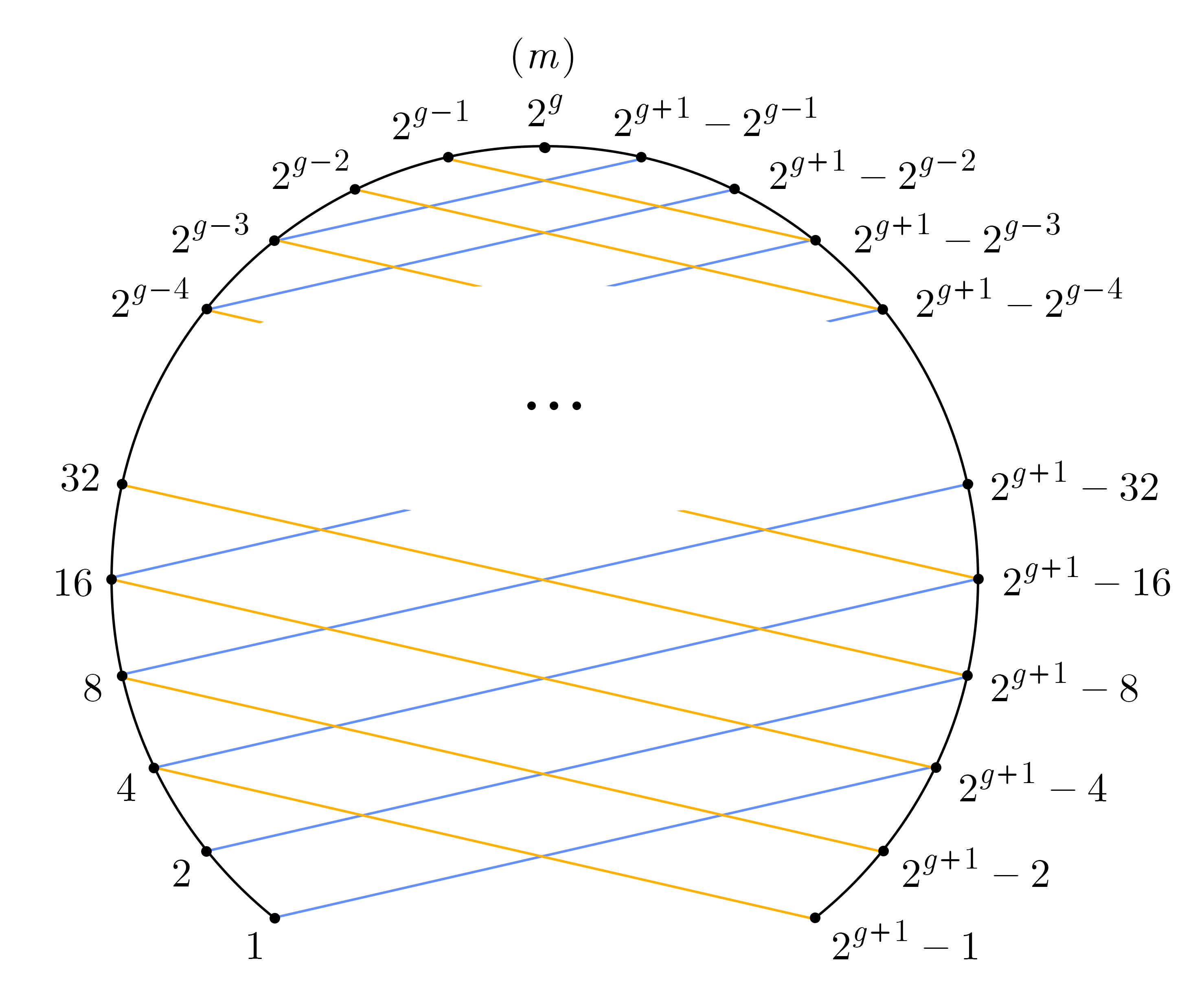
Figure 4: If the blue and yellow edges fail (i.e. all straight-line edges on the inside of the outer semicircle), then we can’t partition the remaining shortest path (black edges along the outer semicircle) into two subpaths that are both $(f-2)$-fault replacement paths.

Proof.

We will first assume for convenience that $f$ is even, and return to the case where $f$ is odd at the end. Let $g=f/2$ and let $G_{f}$ be the graph as illustrated in Figure 4. Formally: the vertices of $G_{f}$ are $1,2\ldots N:=2^{g+1}-1$ (labeled clockwise in Figure 4), and its edge set is $E_{1}\cup E_{2}\cup E_{3}$, where

$$E_{1}:=\{(2^{k},2^{g+1}-2^{k+2}),0\leq k\leq g-3\}$$

$$E_{2}:=\{(2^{k+2},2^{g+1}-2^{k}),0\leq k\leq g-3\}$$

$$E_{3}:=\{(i,i+1),1\leq i\leq N-1\}$$

In the diagram, $E_{1}$ is indicated in blue and slopes upwards to the right, and $E_{2}$ is indicated in yellow and slopes upwards to the left. $E_{3}$ is in black and forms the outer curve. Let $F:=E_{1}\cup E_{2}$, and notice there is a unique replacement path $\pi(1,N\mid F)$ which consists of $E_{3}$, the outer curve. Note that $G_{f}$ is symmetric about the vertex $m=2^{g}$, which is also the midpoint of $\pi(1,N\mid F)$.

Consider any partition of the path $\pi(1,N\mid F)$ into two $(f-1)$-fault replacement paths with fault sets $F_{1}$ and $F_{2}$, and let $x$ be the vertex on which we concatenate them. Label the two subpaths as $\pi(1,x\mid F_{1})$ and $\pi(x,N\mid F_{2})$. Define the “half-arcs” of this graph as $\pi(1,m\mid F)$ and $\pi(m,N\mid F)$, the two subpaths partitioning $\pi(1,N\mid F)$ into equal parts divided at midpoint $m$. (We note that this partitioning will be used again in Lemma 14 as well.)

Any choice of $x$ which divides $\pi(1,N\mid F)$ into two $(f-1)$-fault replacement subpaths will have at least one of the two subpaths entirely contained in one of the half-arcs. Since the construction is symmetric around the vertex $m$, we may assume without loss of generality that $x\geq m$, and $\pi(1,x)$ contains $\pi(1,m\mid F)$.

With this assumption, we will proceed to show that $F_{1}$ must contain every edge in $E_{1}$ and can exclude at most one edge of $E_{2}$, and hence $|F_{1}|\geq f-1$.

First Part ($E_{1}\subseteq F_{1}$).

Consider $\pi(1,x\mid F_{1})$; suppose for a contradiction that there is an edge $(2^{c},2^{g+1}-2^{c+2})\in E_{1}\setminus F_{1}$. Then we can construct a shortcut to $x$ from $1$ by traversing through $(2^{c},2^{g+1}-2^{c+2})$ and then using edges in $E_{3}$ to get to $x$. Explicitly, this path is:

$$\left\{\begin{array}[]{ll}(1,2,\ldots 2^{c})\circ(2^{c},2^{g+1}-2^{c+2})\circ(2^{g+1}-2^{c+2},\ldots x+1,x)&\text{ if }x\leq 2^{g+1}-2^{c+2}\\ (1,2,\ldots 2^{c})\circ(2^{c},2^{g+1}-2^{c+2})\circ(2^{g+1}-2^{c+2},\ldots x-1,x)&\text{ if }x>2^{g+1}-2^{c+2},\end{array}\right.$$

which has length $2^{c}+2^{g+1}-2^{c+2}-x\leq 2^{c}-2^{c+2}+x$ in the first case, or length $2^{c}+2^{c+2}-2^{g+1}+x$ in the second. In either case, the length is strictly less than $x-1$, the length of $\pi(1,x\mid F)$. We must therefore have $E_{1}\subseteq F_{1}$.

Second Part ($|E_{2}\setminus F_{1}|\leq 1$):

For $E_{2}$, suppose for a contradiction that there are two edges of $E_{2}$ which $F_{1}$ does not contain: $(2^{a+2},2^{g+1}-2^{a})$ and $(2^{b+2},2^{g+1}-2^{b})$ with $a<b$. Then in $G\setminus F_{1}$ we have a walk

$$(1,2,\ldots 2^{a+2}) \circ(2^{a+2},2^{g+1}-2^{a})\circ(2^{g+1}-2^{a},2^{g+1}-2^{a}-1,\ldots 2^{g+1}-2^{b})$$

$$\circ(2^{g+1}-2^{b},2^{b+2})\circ(2^{b+2},2^{b+2}+1,\ldots,x-1,x),$$

of length

$$x-3(2^{b}-2^{a})+1<x-1=|\pi(1,x\mid F)|.$$

Thus we must include all of $F$ in $F_{1}$ except at most one edge from $E_{2}$.

Finally, in the case that $f$ is odd, we instead construct $G_{f}$ with $g=\lceil f/2\rceil$, and take any edge out of $E_{1}$ or $E_{2}$, which does not change the analysis. ∎

Our lower bound with two subpaths generalises to our main lower bound result, which we rewrite below:

Proposition 13.

For any $k\in\mathbb{N}$, $(2k,\lfloor{f}/{k}\rfloor-2)$ is not restorable.

Proof.

Assume for convenience that $k$ divides $f$. We will glue $k$ copies of the graph with $f/k$ faults in the previous proposition together, and then show that for any division of a particular $f$-fault replacement path into subpaths, one subpath must contain one of the half-arcs as defined before, and its fault set will have to include $f/k-1$ faults.

We take $k$ copies of $G_{f/k}$ from before, denoted by $G_{1,f/k},G_{2,f/k},\ldots G_{k,f/k}$, labeling the vertices of $G_{i,f/k}$ as $(i,j)$ where $j$ is the label of the corresponding vertex in $G_{f/k}$. We identify each $(i,2^{g+1}-1)$ with $(i+1,1)$. The edges in this graph are the union of all edges of the $G_{i,f/k}$ (see Figure 5), and we define $F$ as the union of the fault sets of each $G_{f/k}$ as defined in the proof of Proposition 12.

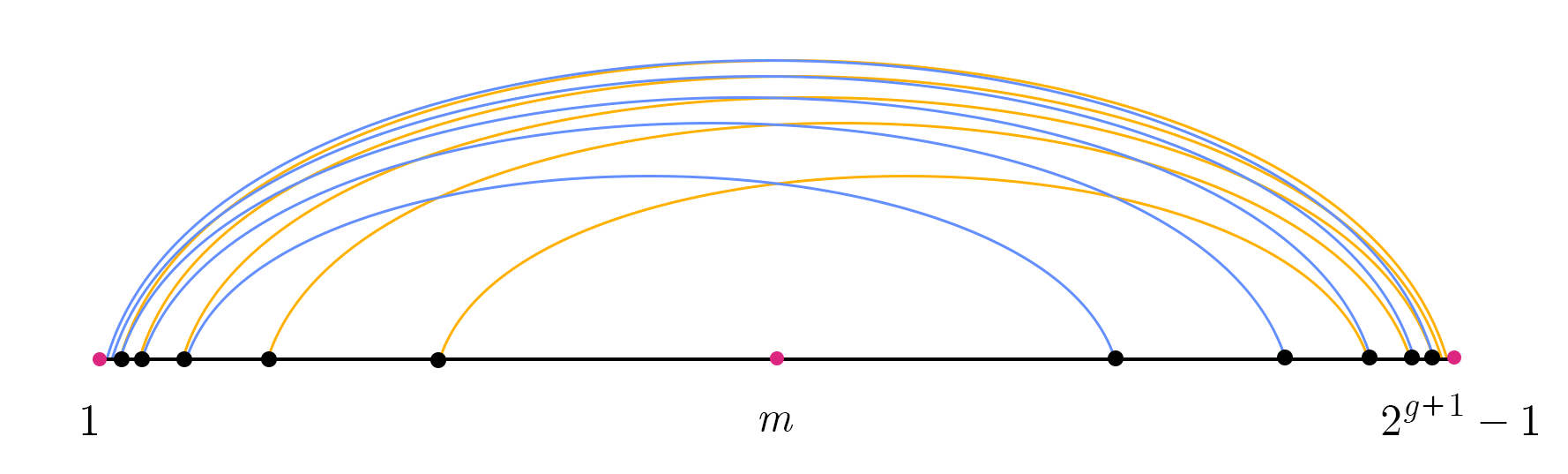
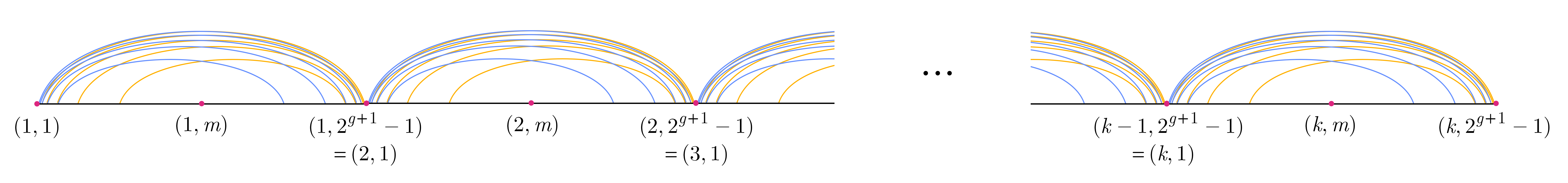
Figure 5: The top figure depicts one copy of $G_{f/k}$, and the bottom depicts all the copies combined together.

Let $E_{j,i}$ denote the $E_{j}$ for $G_{i,f/k}$, so that formally

$$F:=\bigcup_{i=1}^{k}\big{(}E_{1,i}\cup E_{2,i}\big{)}.$$

Let $s:=(1,1)$, $t:=(k,2^{g+1}-1)$. Consider $\pi(s,t\mid F)$. This $f$-fault replacement path is precisely the non-fault edges in $G$, or the union of $E_{3,i}$ over each of the $G_{i,f/k}$.

We now bring in the previous half-arc structure from the case with two subpaths. This graph contains all the half-arcs of each $G_{i,f/k}$, and the half-arcs can be expressed either as $\pi(s,t)[(i,1),(i,m)]$ or $\pi(s,t)[(i,m),(i,2^{g+1}-1)]$. From Proposition 12, we have the following:

Lemma 14.

A path containing a half-arc cannot be a $(f/k-2)$-fault replacement path.

Proof.

Following from the argument of Proposition 12, a fault replacement path containing a half arc of $G_{i,2f/k}$ must have its fault set contain at least every edge in $E_{1,i}\cup E_{2,i}$ except possibly one. Thus any fault set of that path has size at least $f/k-1$. ∎

We will show that any division of $\pi(s,t\mid F)$ into $2k$ subpaths will result in one subpath containing a half-arc, and thus failing to be a $(f/k-2)$-fault replacement path. Suppose we have some choice of boundary vertices $x_{1},x_{2},\ldots x_{2k-1}$ and corresponding fault subsets $F_{1},F_{2},\ldots F_{2k}$, so that each $\pi(s,t)[x_{i-1},x_{i}]$ is a shortest path in $G\setminus F_{i}$.

Let the interior vertices of a path denote all its vertices except its first and last. Note that $\pi(s,t\mid F)$ contains $2k$ half-arcs, and any half-arc which does not have any $x_{i}$ in its interior vertices will be completely contained in some $\pi(s,t)[x_{j-1},x_{j}]$. The interior vertices of all $2k$ half-arcs are disjoint, and we only have $2k-1$ $x_{i}$ which can be in the interior of half arcs. Therefore some subpath $\pi(s,t)[x_{i-1},x_{i}]$ must contain a half-arc, and its fault set $|F_{i}|$ must have size at least $f/k-1$. Thus we will always get that one of the subpaths cannot be a $(f/k-2)$-fault replacement subpath, proving the lower bound.

In the case when $k$ does not divide $f$, we choose graphs which are as even as possible to combine; Let $a$ be the remainder of $f$ divided by $k$. We glue $a$ copies of $G_{\lfloor f/k\rfloor+1}$ to $(k-a)$ copies of $G_{\lfloor f/k\rfloor}$. In this case the subpath which contains a half-arc might contain a half arc of $G_{\lfloor f/k\rfloor}$, and will enforce a fault set of size only $\lfloor f/k\rfloor-1$. ∎

If we want a similar result using this method for the case for an odd number of subpaths, say $2k-1$, we still need to construct $k$ copies of $G_{f/k}$, since half-arcs come in pairs, and we get the same bound on fault sets. Alternatively, we can also use monotonicity to directly get:

Corollary 15.

For any $k\in\mathbb{N}$, $(2k-1,\lfloor{f}/{k}\rfloor-2)$ is not restorable.

4 Upper Bound

We now prove the main result of Theorem 4. Fix any $s,t$ and replacement path $\pi(s,t\mid F)$, where $|F|=:f$. Recall that, to prove Theorem 4, our goal is will show that for any $c\in\mathbb{R}$, we can partition $\pi(s,t\mid F)$ into $O(k)$ $(f/k)$-fault replacement subpaths.

4.1 Subpath Generation

We generate $x_{i}$, the vertices where we split up $\pi(s,t\mid F)$ by traversing along $\pi(s,t\mid F)$ and adding vertices greedily to the current subpath until adding one more vertex would make that subpath no longer a $f/k$-fault replacement path. More precisely, we set $x_{0}:=s$, and then we pick each $x_{i+1}$ to maximize $|\pi(s,t\mid F)[x_{i},x_{i+1}]|$ under the constraint that $\pi(s,t\mid F)[x_{i},x_{i+1}]$ is a $f/k$-fault replacement subpath. Suppose we get $q$ such $x_{i}$, to $x_{q}$. We will denote these $q$ subpaths of $\pi(s,t\mid F)$ by

$$\pi_{i}=\pi(s,t\mid F)[x_{i},x_{i+1}]\quad\forall 0\leq i\leq q-1.$$

Here we remark that the last subpath $\pi_{q-1}$ differs from the others as it is bounded by the end of $\pi(s,t\mid F)$ and is not generated greedily. We will use $\pi^{\prime}_{i}$ to denote the subpaths with one additional vertex included going along the $\pi(s,t\mid F)$ path from $s$ to $t$, for $0\leq i\leq q-2$. We call $\pi_{i}^{\prime}$ the augmented subpaths. Note that no augmented subpath $\pi_{i}^{\prime}$ can be a $f/k$-fault replacement subpath in $G$ by greedy choice of $x_{i}$.

For each $i$, fix $F_{i}$ to be any minimum size fault set such that $\pi^{\prime}_{i}$ is a shortest path in $G\setminus F_{i}$. That is, $\pi^{\prime}_{i}$ is a $|F_{i}|$-fault replacement path but not a $c$-fault replacement path for any $c<|F_{i}|$. By our choice of $x_{i}$, we must have $|F_{i}|\geq f/k+1$. Finally, let $x_{i}^{\prime}$ denote the vertex on $\pi(s,t\mid F)$ immediately after $x_{i}$, so that

$$\pi^{\prime}_{i}=\pi(s,t\mid F)[x_{i},x_{i+1}^{\prime}].$$

Following the notation of [ABDS⁺20], we will denote $\pi_{i}^{\prime}$ as pre-light if its length is less than or equal to the length of $\pi_{i-1}^{\prime}$, and post-light if its length is less than or equal to the length of $\pi_{i+1}^{\prime}$. Also from [ABDS⁺20], at least half of the $\pi_{i}^{\prime}$ are pre-light, or at least half are post-light. We will assume without loss of generality that for at least $\frac{q-1}{2}$ $i$, $\pi_{i}^{\prime}$ is post-light. The other case, where at least half of the $\pi_{i}^{\prime}$ are pre-light, follows from a symmetric argument.

4.2 FS-pair Generation

Next, we generate a set of FS-pairs. The following process specifically generates right FS-pairs; this is because we assume above that most subpaths are post-light. If in the other case, where most subpaths are pre-light, we would instead generate left FS-pairs through a symmetric process.

FS-pairs are denoted by $(e^{*},\pi_{i}^{\prime})$, where $e^{*}$ is a fault in $F$, and $\pi_{i}^{\prime}$ is a post-light augmented subpath. Every FS-pair has the property that there exists a fault-free path from the right end $x^{\prime}_{i+1}$ of $\pi_{i}^{\prime}$ to $e^{*}$. Before we generate these, we will set up some notation.

Definition 16.

For any $u,v$-path $p^{\prime}$, we say a $u,v$-path $p$ is a shortcut of $p^{\prime}$ if $\text{len}(p)<\text{len}(p^{\prime})$.

Fix any post-light augmented subpath $\pi_{i}^{\prime}$. For a given $e\in F_{i}$ which we refer to as the generating fault, let $S_{e}$ be the set of $x_{i+1}^{\prime},x_{i}$ shortcuts for $\pi_{i}^{\prime}$ which contain $e$. For a shortcut $p\in S_{e}$, we define the base fault $b(p)\in F$ of $p$ as the first fault in $p$ from $x_{i+1}^{\prime}$ to $x_{i}$. More precisely, we define

$$b(p):=e_{\min\{j:e_{j}\in F\}}\text{ where }p=x_{i+1}^{\prime}e_{1}v_{1}e_{2}\ldots e_{m}x_{i}.$$

For each $e\in F_{i}$, we define its set of base faults for $\pi_{i}^{\prime}$ as

$$B(e):=\{b(p):p\in S_{e}\}$$

Finally, we define the family of base faults for $\pi_{i}^{\prime}$ as

$$\mathcal{B}(\pi_{i}^{\prime})=\{B(e):e\in F_{i}\}$$

Our next goal will be to choose a distinct base fault from each base fault set $B(e)\in\mathcal{B}(\pi_{i}^{\prime})$ in order to define the FS-pairs.

Explicitly, we define an auxiliary bipartite graph $\Gamma_{i}$ where one side of the bipartition is $F_{i}$ and the other is the set of faults $F$, and where $(e,e^{*})\in E(\Gamma_{i})$ iff $e^{*}\in B(e)$. In this set up, choosing a distinct base fault for each $B(e)$ is equivalent to finding a matching of $\Gamma_{i}$ which saturates $F_{i}$. Hall’s Theorem gives us a condition for this:

Lemma 17 (Hall’s Condition).

If for every $A\subseteq F_{i}$ we have $|N(A)|\geq|A|$, where $N(A)$ is the neighborhood of $A$ in $\Gamma_{i}$, then $\Gamma_{i}$ contains a matching that saturates $F_{i}$ (and therefore it is possible to choose a distinct base fault for each $B(e)$).

We therefore only need to verify the premises of Hall’s Condition. The following lemma will be helpful.

Lemma 18.

For any $A\subseteq F_{i}$, the fault set $F^{\prime}_{i}:=F_{i}\setminus A\cup N(A)$ is also a valid fault set for $\pi_{i}^{\prime}$. (That is, $\pi_{i}^{\prime}$ is a shortest path in $G\setminus F^{\prime}_{i}$.)

Proof.

First, we observe that

$$N(A)=\left|\bigcup_{e\in A}B(e)\right|.$$

This holds because the neighbours of each generating fault $e$ is the set of base faults $B(e)$ it generates.

We now need to prove that no shortcuts for $\pi_{i}^{\prime}$ survive in $G\setminus F^{\prime}_{i}$. Let $p$ be an arbitrary shortcut for $\pi_{i}^{\prime}$ in $G$. Then it must contain some fault $e^{\prime}\in F_{i}$, since $F_{i}$ is a valid fault set. There are two cases:

• If $e^{\prime}\in F^{\prime}_{i}$, then the shortcut $p$ does not survive in $G\setminus F^{\prime}_{i}$.

• Otherwise, suppose that $e^{\prime}\notin F^{\prime}_{i}$, and so in particular $e^{\prime}\in A$. In this case, $p$’s base fault $b(p)$ is in $B(e^{\prime})\subseteq F^{\prime}_{i}$, and thus not in $G\setminus F^{\prime}_{i}$.

Therefore there are no surviving shortcuts for $\pi_{i}^{\prime}$ in $G\setminus F^{\prime}_{i}$. ∎

Notice that Lemma 17 follows from Lemma 18: since we assume that $F_{i}$ is a minimal fault set, we must have that $|N(A)|\geq A$ for all $A\subseteq F_{i}$, since otherwise we would have $|F^{\prime}_{i}|<|F_{i}|$. Since Hall’s condition holds, over any augmented subpath $\pi_{i}^{\prime}$, we can assign a unique base fault to every generating fault. Accordingly, we can define an injective function $\phi_{i}:F_{i}\to F$ where $\phi_{i}(e)\in B(e,\pi_{i}^{\prime})$.

We will construct our FS-pairs for $\pi_{i}^{\prime}$ as $\{(\phi_{i}(e),\pi_{i}^{\prime})\mid e\in F_{i}\}$, and repeat this process for every post-light augmented subpath. It follows that we will generate at least $(q-1)f/(2k)$ FS-pairs, since we have $(q-1)/2$ post-light augmented subpaths which have corresponding fault sets $F_{i}$ with at least $f/k$ faults, each of which can be assigned to one unique base fault in context of the augmented subpath.

4.3 Analysis of FS-pairs

Lemma 19.

Each fault in $F$ will be in at most 4 FS-pairs.

Proof.

Recall that only post-light $\pi_{i}^{\prime}$ will be in FS-pairs. Suppose, for a contradiction, that there is some base fault $e=(u,v)$ associated with 5 $\pi_{i}^{\prime}$. Then without loss of generality, at least 3 of the $\pi_{i}^{\prime}$ have fault-free paths as subsets of some shortcut from their right ends $x_{i+1}^{\prime}$ to $u$. Let these subpaths be $\pi_{a}^{\prime}$, $\pi_{b}^{\prime}$, and $\pi_{c}^{\prime}$, with $a<b<c$. We will also label the fault-free paths as $p_{a}$, $p_{b}$, and $p_{c}$. We have

$$|p_{a}|\leq|\pi_{a}^{\prime}|-2\quad\text{and}\quad|p_{c}|\leq|\pi_{c}^{\prime}|-2$$

since the shortcut of $\pi_{a}^{\prime}$ which $p_{a}$ is on has length at least $|p_{a}|+1$ when we include $e$, and same with $p_{c}$.

Since $\pi_{a}^{\prime}$ is post-light, we have

$$|\pi_{a+1}^{\prime}|\geq|\pi_{a}^{\prime}|.$$

With each $\pi_{i}^{\prime}$ being extended from $\pi_{i}$ by one vertex, we have also

$$|\pi_{a+1}|\geq|\pi_{a}|.$$

Moreover, since $a<b<c$, $a+1\neq c$. Note that the distance from $x_{a+1}^{\prime}$ to $x_{c+1}^{\prime}$ in $G\setminus F$ is their distance along any shortest path they’re both on, which gives us a lower bound of

$$d_{G\setminus F}(x_{a+1}^{\prime},x_{c+1}^{\prime}) =\pi(s,t\mid F)[x_{a+1}^{\prime},x_{c+1}^{\prime}]$$

$$=\sum_{i=a+1}^{c}|\pi_{i}|$$

$$\geq|\pi_{a+1}|+|\pi_{c}|$$

$$\geq|\pi_{a}|+|\pi_{c}|.$$

However, $p_{a}$ and $p_{c}$ give a fault-free path from $x_{a+1}^{\prime}$ to $x_{c+1}^{\prime}$ also, which upper bounds their distance as

$$d_{G\setminus F}(x_{a+1}^{\prime},x_{c+1}^{\prime}) \leq d_{G\setminus F}(x_{a+1}^{\prime},u)+d_{G\setminus F}(u,x_{c+1}^{\prime})$$

$$\leq|p_{a}|+|p_{c}|$$

$$\leq|\pi_{a}^{\prime}|+|\pi_{c}^{\prime}|-4$$

$$=|\pi_{a}|+|\pi_{c}|-2.$$

Which contradicts $\pi(s,t\mid F)$ being a shortest path. Therefore, each base fault in $F$ is associated with at most 4 $\pi_{i}^{\prime}$ over all FS-pairs. ∎

We are now ready to finish the proof of Theorem 4. Since we can generate $\frac{(q-1)f}{2k}$ FS-pairs, each base fault can only be in 4 FS-pairs, and there are at most $f$ possible choice of base faults, we have

$$4f\geq\frac{(q-1)f}{2k}\implies q\leq 8k+1.$$

Corollary 20.

For any partition of $\pi(s,t\mid F)$ into subpaths $\pi_{i}$, there are at most $4f$ right FS-pairs containing post-light augmented subpaths $\{\pi_{i}^{\prime}\}$.

Again, in the other case where most subpaths are pre-light, the relevant corollary is that there are at most $4f$ left FS-pairs containing pre-light augmented subpaths $\{\pi_{i}^{\prime}\}$. The proof is essentially identical.

5 Weighted Upper Bound

We next prove Theorem 6. Recall that the goal is to prove that in any weighted graph $G$, every $f$-fault replacement path $\pi$ can be partitioned into

$$\pi=\pi_{0}\circ e_{0}\circ\pi_{1}\circ e_{1}\circ\dots\circ e_{q-2}\circ\pi_{q-1}$$

where each $e_{i}$ is an edge and each $\pi_{i}$ is a (possibly empty) subpath of $\pi$ that is an $(f/k)$-fault replacement path in $G$, with $q=O(k)$.

Our proof strategy will be similar to the previous argument with some minor changes: we still choose $\pi_{i}$ greedily as the longest subpath which is an $(f/k)$-fault replacement path, and we will take the next edge in the subpath as the $e_{i}$ to interweave. Let $q$ be the number of subpaths resulting from this decomposition; our goal is to upper bound $q$ to be linear in $k$.

We will define $\pi_{i}^{\prime}$ as $\pi_{i}$ augmented with $e_{i}$ (again $\pi^{\prime}_{q}$ is undefined). We define $x_{i}$ as the vertex at the end of $\pi_{i-1}^{\prime}$ and at the beginning of $\pi_{i}$, so that for any $i$,

$$\pi(s,t\mid F)[x_{i},x_{i+1}]=\pi_{i}^{\prime}=\pi_{i}\circ e_{i}.$$

Unlike in the unweighted setting, we no longer have overlaps in the $\pi_{i}^{\prime}$. We will assess whether subpaths $\pi_{i}^{\prime}$ are pre-light or post-light based on their weighted length, and proceed supposing that at least half of the subpaths are post-light. We generate FS-pairs with post-light subpaths as before, using the property that by maximality of $\pi_{i}$, each $\pi_{i}^{\prime}$ necessarily fails to be an $(f/k)$-fault replacement path. Using the same argument based on Hall’s Theorem as before, this guarantees that we get at least $\frac{(q-1)f}{2k}$ distinct FS-pairs. Now we can complete the proof of Theorem 6 by the following lemma, which is analogous to Lemma 19, and will be proved similarly.

Lemma 21.

Each (weighted) fault in $F$ will be in at most 4 FS-pairs.

Proof.

Similarly to Lemma 19 we will prove the lemma by showing that no fault can be in 5 FS-pairs. Suppose, for a contradiction, that we have fault $e=(u,v)$ in 5 FS-pairs. Without loss of generality at least 3 subpaths $\pi_{a}^{\prime}$, $\pi_{b}^{\prime}$, and $\pi_{c}^{\prime}$ have fault-free paths which are contained in shortcuts from their right ends $x_{a+1}$, $x_{b+1}$, and $x_{c+1}$ to $u$. Let these paths be $p_{a}$, $p_{b}$, and $p_{c}$. Since each path is contained in a shortcut using $e$, we have

$$w(p_{a})<w(\pi_{a}^{\prime})-w(e)\quad\text{and}\quad w(p_{c})<w(\pi_{c}^{\prime})-w(e).$$

Since $\pi_{a}^{\prime}$ is post-light, we have

$$w(\pi_{a+1}^{\prime})\geq w(\pi_{a}^{\prime}).$$

Again we can use that $a+1<c$ and that $\pi(s,t\mid F)$ is a shortest path to lower bound the weighted distance of $x_{a+1}$ to $x_{c+1}$ in $G\setminus F$ as

$$d_{G\setminus F}(x_{a+1},x_{c+1}) =w(\pi(s,t\mid F)[x_{a+1},x_{c+1}])$$

$$=\sum_{i=a+1}^{c}w(\pi_{i}^{\prime})$$

$$\geq w(\pi_{a+1}^{\prime})+w(\pi_{c}^{\prime})$$

$$\geq w(\pi_{a}^{\prime})+w(\pi_{c}^{\prime}).$$

However we can use the fault free paths of $p_{a}$ and $p_{c}$ to upper bound the distance from $x_{a+1}$ to $x_{c+1}$ in $G\setminus F$ to get a contradiction with the previous lower bound:

$$d_{G\setminus F}(x_{a+1},x_{c+1}) \leq d_{G\setminus F}(x_{a+1},u)+d_{G\setminus F}(u,x_{c+1})$$

$$\leq w(p_{a})+w(p_{c})$$

$$<w(\pi_{a}^{\prime})+w(\pi_{c}^{\prime})-2w(e).$$ ∎

In the case that at least half of the subpaths are pre-light, we will generate FS-pairs with pre-light subpaths by defining base faults relative to the left ends $x_{i}$ of subpaths $\pi_{i}^{\prime}$. In the analysis, we replace $x_{a+1}$, $x_{b+1}$, and $x_{c+1}$ with $x_{a}$, $x_{b}$ and $x_{c}$. Our analysis of $p_{a}$, $p_{b}$, and $p_{c}$ are unchanged. Comparing subpaths, we instead use the pre-light property of $\pi_{c}^{\prime}$ to get

$$w(\pi_{c-1}^{\prime})\geq w(\pi_{c}^{\prime}).$$

Then the analysis on the distance is a lower bound of

$$d_{G\setminus F}(x_{a},x_{c}) =w(\pi(s,t\mid F)[x_{a},x_{c}])$$

$$=\sum_{i=a}^{c-1}w(\pi_{i}^{\prime})$$

$$\geq w(\pi_{a}^{\prime})+w(\pi_{c-1}^{\prime})$$

$$\geq w(\pi_{a}^{\prime})+w(\pi_{c}^{\prime}),$$

and an upper bound of

$$d_{G\setminus F}(x_{a},x_{c}) \leq d_{G\setminus F}(x_{a},u)+d_{G\setminus F}(u,x_{c})$$

$$\leq w(p_{a})+w(p_{c})$$

$$<w(\pi_{a}^{\prime})+w(\pi_{c}^{\prime})-2w(e).$$

6 Algorithmic Path Decomposition

We will next prove Theorem 7, which holds for unweighted input graphs, and then afterwards describe the (minor) changes needed to adapt the algorithm to the weighted setting. As a reminder of our goal: we are given a graph $G$, a fault set $F$, a replacement path $\pi(s,t\mid F)$, and a parameter $k$ on input. Our goal is to find nodes $\{x_{i}\}$ and fault sets $F_{i}$, which partitions $\pi(s,t\mid F)$ into $q=O(k)$ replacement paths avoiding $f/k$ faults each, as

$$\pi(s,t\mid F)=\pi(x_{0},x_{1}\mid F_{1})\circ\pi(x_{1},x_{2}\mid F_{2})\circ\ldots\circ\pi(x_{q-1},x_{q}\mid F_{q}).$$

6.1 Fault Set Reducing Subroutine

Before describing our main algorithm, we will start with a useful subroutine, driven by an observation about the matching step in FS-pair generation. In our upper bound proof, we used a process for generating FS-pairs to bound the number of subpaths in the decomposition. We used minimum size of the fault set $F_{i}$ associated to each augmented subpath $\pi_{i}^{\prime}$ to argue that we could generate $|F_{i}|$ distinct FS-pairs.

The observation is that, letting $F_{i}$ be any (not necessarily minimum) valid fault set for $\pi_{i}^{\prime}$ (that is, $\pi_{i}^{\prime}$ is a shortest path in $G\setminus F_{i}$), if we can produce an FS-pair for every fault in $F_{i}$ then our previous argument works. On the other hand, if we cannot produce an FS-pair for every fault in $F_{i}$, then our previous argument gives us a process by which we can find a strictly smaller fault set $F_{i}^{\prime}$ that is also valid for $\pi_{i}^{\prime}$, by replacing the subset of $F_{i}$ with the reduced set of their base faults.

The subroutine FaultReduce runs this process iteratively, in order to find a fault set $F_{i}$ for the input subpath $\pi_{i}$ that can be used to generate $|F_{i}|$ FS-pairs (from both the left and right). We note the subtlety that $F_{i}$ is not necessarily a minimum valid fault set for $\pi_{i}$: as in Figure 6, there may exist a smaller valid fault set, but the algorithm will halt nonetheless if it can certify that the appropriate number of FS-pairs can be generated.

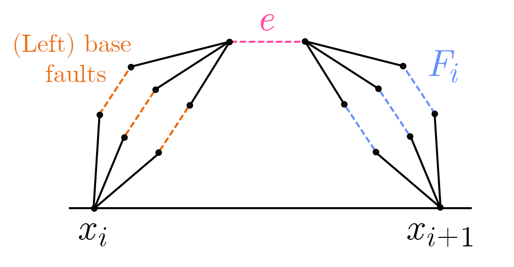
Figure 6: This subpath and fault set $F_{i}$ produces multiple FS-pairs via a saturated matching using the faults on the left as base faults, but its minimum fault set is only one edge $\{e\}$.

Algorithm 1 FaultReduce $(\pi_{i})$

$F_{i}\leftarrow F$

Construct $\Gamma_{L}$.

Construct $\Gamma_{R}$.

loop

     Compute max matching $M_{L}$ for $F_{i}$ in $\Gamma_{L}$.

     Compute max matching $M_{R}$ for $F_{i}$ in $\Gamma_{R}$.

     if $|M_{L}|<|F_{i}|$ or $|M_{R}|<|F_{i}|$ then

         Reduce $F_{i}$

     else return $F_{i}$      

The essential properties of Algorithm 1 are captured by the following lemma.

Lemma 22.

Relative to a graph $G$ and fault set $F$, there is a subroutine (Algorithm 1 - FaultReduce) that runs in polynomial time with the following behavior:

• The input is a path $\pi_{i}$ that is a shortest path in $G\setminus F$.

• The output is a fault set $F_{i}\subseteq F$, such that:

  • $\pi_{i}$ is a shortest path in $G\setminus F_{i}$, and

  • one can generate $|F_{i}|$ left- and $|F_{i}|$ right-FS-pairs of $\pi_{i}$ from $F_{i}$.

We will next provide additional details on some of the steps in Algorithm 1, and then prove Lemma 22.

Construction of $\Gamma_{L}$ and $\Gamma_{R}$.

As in our previous proof, the graphs $\Gamma_{L},\Gamma_{R}$ are the graphs representing the association between faults in $F_{i}$ and left or right (respectively) base faults in $F$. More specifically:

• Both $\Gamma_{L}$ and $\Gamma_{R}$ are bipartite graphs with vertex set $F_{i}\cup F$, where $F_{i}$ is the current fault set, and $F$ is all initial faults.

  Thus faults in $F_{i}$ are represented by two vertices, one on each side of the bipartition.

• In $\Gamma_{L}$, we place an edge from $e\in F_{i}$ to $e_{b}\in F$ iff $e_{b}$ is a left base fault for $e$. The edges of $\Gamma_{R}$ are defined similarly, with respect to right base faults.

These graph constructions require us to efficiently check whether or not a particular fault $e_{b}\in F$ acts as a (left or right) base fault for some $e\in F_{i}$. We next describe this process:

Lemma 23.

Given a subpath $\pi_{i}$, a valid fault set $F_{i}$, and faults $e\in F_{i},e_{b}\in F$, we can check whether or not $e_{b}$ is a left and/or right base fault of $e$ in polynomial time.

Proof.

First, the following notation will be helpful. Let $x_{i},x_{i+1}$ be the endpoints of the input subpath $\pi_{i}$. We will write $d(x_{i},x_{i+1}\mid e_{b}\leadsto e)$ for the length of the shortest (possibly non-simple) $(x_{i},x_{i+1})$-path that contains both $e_{b}$ and $e$, and which specifically uses $e$ as the first fault in $F$ along the path. We define $d(x_{i+1},x_{i}\mid e_{b}\leadsto e)$ similarly. Note that $e_{b}$ is a left base fault for $e$ iff

$$d(x_{i},x_{i+1}\mid e_{b}\leadsto e)<|\pi_{i}|$$

and that $e_{b}$ is a right base fault for $e$ iff

$$d(x_{i+1},x_{i}\mid e_{b}\leadsto e)<|\pi_{i}|.$$

Thus, it suffices to compute the values of the left-hand side of these two inequalities. We will next describe computation of $d(x_{i},x_{i+1}\mid e_{b}\leadsto e)$; the other computation is symmetric. There are two cases, depending on whether or not $e_{b}=e$. Let $e=(u,v)$, $e_{b}=(u_{b},v_{b})$. When $e_{b}\neq e$, the formula is:

$$d(x_{i},x_{i+1}\mid e_{b}\leadsto e)=\min\{ d_{G\setminus F}(x_{i},u_{b})+d_{G}(v_{b},u)+d_{G}(v,x_{i+1})+2,$$

$$d_{G\setminus F}(x_{i},u_{b})+d_{G}(v_{b},v)+d_{G}(u,x_{i+1})+2,$$

$$d_{G\setminus F}(x_{i},v_{b})+d_{G}(u_{b},u)+d_{G}(v,x_{i+1})+2,$$

$$d_{G\setminus F}(x_{i},v_{b})+d_{G}(u_{b},v)+d_{G}(u,x_{i+1})+2\}.$$

The four parts are needed since we consider paths that use $e,e_{b}$ with either orientation, and the $+2$ term arises to count the contribution of the edges $e,e_{b}$ themselves. In the case where $e_{b}=e$, the formula is

$$d(x_{i},x_{i+1}\mid e\leadsto e) =\min\{d_{G\setminus F}(x_{i},u)+d_{G}(v,x_{i+1})+1,d_{G\setminus F}(x_{i},v)+d_{G}(u,x_{i+1})+1\}.$$ ∎

Reducing $F_{i}$.

Next, we provide more detail on the step of reducing the fault set $F_{i}$. This uses Hall’s condition, in an analogous way to our previous proof. When we compute max matchings $M_{L},M_{R}$ for $\Gamma_{L},\Gamma_{R}$, if we successfully find matchings of size $|M_{L}|\geq|F_{i}|$ or $|M_{R}|\geq|F_{i}|$, then we have certified the ability to generate $|F_{i}|$ left and right FS-pairs as in Section 4.2, and so the algorithm can return $F_{i}$ and halt. Otherwise, suppose without loss of generality that $|M_{L}|<|F_{i}|$. By Hall’s condition, that means there exists a fault subset $A\subseteq F_{i}$ such that the set of base faults $B\subseteq F$ used by faults in $A$ is strictly smaller than $A$ itself. For the reduction step, we set $F_{i}\leftarrow F_{i}\cup B\setminus A$, which reduces the size of $|F_{i}|$. By Lemma 18, this maintains the invariant that $F_{i}$ is a valid fault set for the input path $\pi_{i}$.

In order to efficiently find the non-expanding fault subset $A\subseteq F_{i}$, we may compute the max matching in $\Gamma_{L}$ (or $\Gamma_{R}$) using a primal-dual algorithm that returns both a max matching and a certificate of maximality of this form. For example, the Hungarian algorithm will do [CLRS09].

6.2 Main Algorithm

ComputeSubpaths, described in Algorithm 2, performs a greedy search for subpath boundaries. In each round, we set the next subpath boundary node $x_{i+1}$ to be the furthest node from the previous subpath boundary node $x_{i}$, such that the corresponding subpath is certified by the algorithm FaultReduce to have size $\leq f/k$. Thus, considering the augmented subpath that we get by adding an additional node to $\pi_{i}$, we can generate $>f/k$ left and right FS-pairs from this subpath.

We next state the algorithm; for ease of notation we label the vertices of the input path $\pi(s,t\mid F)$ as $v_{0},v_{1},\ldots,v_{\ell}$.

Algorithm 2 ComputeSubpaths $(\pi(s,t\mid F),F,k)$

$x_{0}\leftarrow s$.

$i\leftarrow 0$.

while $x_{i}\neq v_{\ell}$ do

     Binary search for largest $y$ such that the fault set returned by FaultReduce$(\pi(s,t)[x_{i},v_{y}])$ has size $\leq f/k$.

     $i\leftarrow i+1$.

     $x_{i}\leftarrow v_{y}$.

return $\{x_{j}\}_{j=0}^{i}$

Theorem 24.

Algorithm 2 is correct and runs in polynomial time.

Proof.

In Corollary 20 from our upper bound section, we showed that there exist only $O(f)$ total right FS-pairs using post-light subpaths (and, symmetrically, there exist only $O(f)$ left FS-pairs using pre-light subpaths). Since at least half of the augmented subpaths are pre-light or half are post-light, and by Lemma 22 every augmented subpath can generate at least $f/k$ left and right FS-pairs, altogether we will have at most $O(k)$ subpaths.

For runtime, we always generate a linear number of subpaths, and locating the endpoint of each requires calling the subroutine $\log n$ times. Thus the entire algorithm runs in polynomial time. ∎

A similar approach works in the weighted setting, since the method of counting FS-pairs extends to the structure in Theorem 6 and upper bounds the number of interweaved subpaths and edges. The construction of auxiliary graphs $\Gamma_{L}$ and $\Gamma_{R}$ requires checking the weighted distance, but the matching and FS-pair generation is the same. We change the algorithm to add the next edge into the decomposition of $\pi(s,t\mid F)$ after finding a maximal subpath with fault set at most $f/k$. The upper bound for the number of subpaths based on enough FS-pairs being generated follows from the analysis in Theorem 6.

References

- [ABDS+20] Reyan Ahmed, Greg Bodwin, Faryad Darabi Sahneh, Stephen Kobourov, and Richard Spence. Weighted additive spanners. In Isolde Adler and Haiko Müller, editors, Graph-Theoretic Concepts in Computer Science, pages 401–413, Cham, 2020. Springer International Publishing.
- [BBAK+01] Anat Bremler-Barr, Yehuda Afek, Haim Kaplan, Edith Cohen, and Michael Merritt. Restoration by path concatenation: Fast recovery of mpls paths. In Proceedings of the Twentieth Annual ACM Symposium on Principles of Distributed Computing, PODC ’01, page 43–52, New York, NY, USA, 2001. Association for Computing Machinery.
- [BCG+18] Davide Bilò, Keerti Choudhary, Luciano Gualà, Stefano Leucci, Merav Parter, and Guido Proietti. Efficient oracles and routing schemes for replacement paths. In 35th Symposium on Theoretical Aspects of Computer Science (STACS 2018). Schloss Dagstuhl-Leibniz-Zentrum fuer Informatik, 2018.
- [BGPW17] Greg Bodwin, Fabrizio Grandoni, Merav Parter, and Virginia Vassilevska Williams. Preserving Distances in Very Faulty Graphs. In Ioannis Chatzigiannakis, Piotr Indyk, Fabian Kuhn, and Anca Muscholl, editors, 44th International Colloquium on Automata, Languages, and Programming (ICALP 2017), volume 80 of Leibniz International Proceedings in Informatics (LIPIcs), pages 73:1–73:14, Dagstuhl, Germany, 2017. Schloss Dagstuhl–Leibniz-Zentrum fuer Informatik.
- [BP21] Greg Bodwin and Merav Parter. Restorable shortest path tiebreaking for edge-faulty graphs. In Proceedings of the 2021 ACM Symposium on Principles of Distributed Computing, PODC’21, page 435–443, New York, NY, USA, 2021. Association for Computing Machinery.
- [CC19] Shiri Chechik and Sarel Cohen. Near optimal algorithms for the single source replacement paths problem. In Proceedings of the Thirtieth Annual ACM-SIAM Symposium on Discrete Algorithms, pages 2090–2109. SIAM, 2019.
- [CCFK17] Shiri Chechik, Sarel Cohen, Amos Fiat, and Haim Kaplan. (1+)-approximate f-sensitive distance oracles. In Proceedings of the Twenty-Eighth Annual ACM-SIAM Symposium on Discrete Algorithms, pages 1479–1496. SIAM, 2017.
- [CLRS09] Thomas H. Cormen, Charles E. Leiserson, Ronald L. Rivest, and Clifford Stein. Introduction to Algorithms, 3rd Edition. MIT Press, 2009.
- [GJM20] Manoj Gupta, Rahul Jain, and Nitiksha Modi. Multiple source replacement path problem. In Proceedings of the 39th Symposium on Principles of Distributed Computing, pages 339–348, 2020.
- [HS01] John Hershberger and Subhash Suri. Vickrey prices and shortest paths: What is an edge worth? In Proceedings 42nd IEEE symposium on foundations of computer science, pages 252–259. IEEE, 2001.
- [MMG89] Kavindra Malik, Ashok K Mittal, and Santosh K Gupta. The k most vital arcs in the shortest path problem. Operations Research Letters, 8(4):223–227, 1989.