Morphological stability for in silico models of avascular tumors

Abstract

The landscape of computational modeling in Cancer Systems Biology is diverse, offering a spectrum of models and frameworks, each with its own trade-offs and advantages. Ideally, models are meant to be useful in refining hypotheses, to sharpen experimental procedures and, in the longer run, even for applications in personalized medicine. One of the greatest challenges is to balance model realism and detail with experimental data to eventually produce useful data-driven models.

We contribute to this quest by developing a transparent, highly parsimonious, first principle in silico model of a growing avascular tumor. We initially formulate the physiological considerations and the specific model within a stochastic cell-based framework. We next formulate a corresponding mean-field model using partial differential equations which is amenable to mathematical analysis. Despite a few notable differences between the two models, we are in this way able to successfully detail the impact of all parameters in the stability of the growth process and on the eventual tumor fate of the stochastic model. This facilitates the deduction of Bayesian priors for a given situation, but also provides important insights into the underlying mechanism of tumor growth and progression.

Although the resulting model framework is relatively simple and transparent, it can still reproduce the full range of known emergent behavior. We identify a novel model instability arising from nutrient starvation and we also discuss additional insight concerning possible model additions and the effects of those. Thanks to the framework’s flexibility, such additions can be readily included whenever the relevant data become available.

Keywords: Computational tumorigenesis, Cell population modeling, Emergent property, Darcy’s law, Saffman-Taylor instability.

AMS subject classification: Primary: 35B35, 92C10; secondary: 65C40, 92-08.

Statements and Declarations: This work was partially funded by support from the Swedish Research Council under project number VR 2019-03471. The authors declare no competing interests.

1 Introduction

Tumors are highly complicated biological systems, yet constitute a concrete example of cellular self-organization processes amenable to modeling in silico [6]. In a cancerous tumor, the cells have undergone several significant mutations and obtained distinct hallmarks providing the population with remarkable growth capabilities [20, 21]. Furthermore, populations comprising large numbers of cells interact on multiple scales, yielding a range of emergent phenomena [10], which can be studied using computational models based on knowledge of single-cell behavior. To the modeler’s aid in this regard, biological data streams nowadays contain detailed features at the individual cell level such as cell size and -type, mutation- and growth rate, molecular constituents, and gene expression [28, 8, 1].

Complementing biological experiments, mathematical models can in addition provide explanations to observed data, concerning, e.g., drug-response in tumor growth, with potential applications in precision medicine [36, 3]. Progress in Cell Biology has led to a good understanding of intra-cellular processes which unlocks the possibility to model these systems from fundamental principles, to translate ‘word models’ formulated from biological experiments into mathematical and computational models, and to test the features of these models [27]. Often quoted uses of computational models include the testing of hypotheses, the investigation of causality, and the integration of knowledge when comparing in vitro and in vivo data [5]. Bayesian inference methods present a means to quantitatively investigating these matters, provided there exist appropriate data and meaningful priors associated with the model parameters.

Several cell population models exist in the literature, ranging from continuous to agent-based to hybrid models, and taking place at various scales [30, 11, 14, 32]. Such models may reach a predictive power, where agreement/disagreement with biological data can advance our understanding of mechanistic relations within the biological systems [22, 16, 4, 12]. Pertinent to the present work, previous research shows how analyzing the emergent morphology of cell population models can provide insight into the role of the model parameters [17], promoting future use of Bayesian methods. Such analysis has, for example, enabled modelers to analyze the behavior of the invasive fronts of tumor models and their response to parameter changes representing vascularization, nutrient availability [9, 23], and cell-cell adhesion effects [7, 31].

Motivated in part by improvements of in vitro techniques for obtaining detailed time-series tumor and single-cell data and the current trend in Computational Science towards data-driven modeling, we present and analyze a basic continuous mathematical model of avascular tumor growth, here derived from a previously developed cell-based model [13]. Our aim is that the model should be highly parsimonious in order to cope with issues of model identifiability. For this purpose the in silico tumor’s fate should be well understood when regarded as a map from parameters to simulation end-result. Initial results from an earlier version of the model [13] display boundary instabilities, akin to those discussed in [18], which we analyze thoroughly. The self-regulating properties of avascular tumors concerning size that have been observed in vitro [15] and in silico [19] motivate a careful investigation into the model capabilities in this regard.

We have structured the paper as follows. In §2 we summarize the stochastic cell-based tumor model as well as the associated mean-field space-continuous version. We analyze the latter in §3, assuming a radially symmetric solutions first, and then via linear stability analysis. In §4 we highlight via some numerical examples the sharpness of the analysis as well as its relevance for the stochastic model. A concluding discussion is found in §5.

2 Stochastic modeling of avascular tumors

An advantage held by stochastic models is that they implicitly define a consistent likelihood and thus formally have the potential to be employed in Bayesian modeling when confronted with data. We summarize our stochastic framework in §2.1 and the basic stochastic tumor model in §2.2. We next derive a corresponding mean-field version in §2.3, which has the distinct advantage of being open to a mathematical analysis.

2.1 Stochastic framework

The Darcy Law Cell Mechanics (DLCM) framework [13] is a cell-based stochastic modeling framework where the cells are explicitly represented and the rates of their state updates, e.g., movement, proliferation, death, etc., are determined and govern the corresponding events in a continuous-time Markov chain. Movements of the cells generally follow Darcy’s law for fluid flow in a porous environment, but since the framework takes place in continuous time, other types of cell transport are easily incorporated.

The spatial domain is discretized into $i=1,2,...,N_{\text{vox}}$ voxels $v_{i}$, and populated by a total of $N_{\text{cells}}$ cells. The DLCM framework can be used over any grid for which a consistent discrete Laplace operator can be derived. Each voxel may be empty or contain some number of cells and if this number exceeds the voxel’s carrying capacity, the cells will exert a pressure onto the cells in the surrounding voxels, see Fig. 2.1. The pressure propagates through the considered domain and the local pressure gradient induces a cell flow. The simplest implementation allows each voxel to be populated by $u_{i}\in\{0,1,2\}$ cells at any time, thus with a carrying capacity of 1.

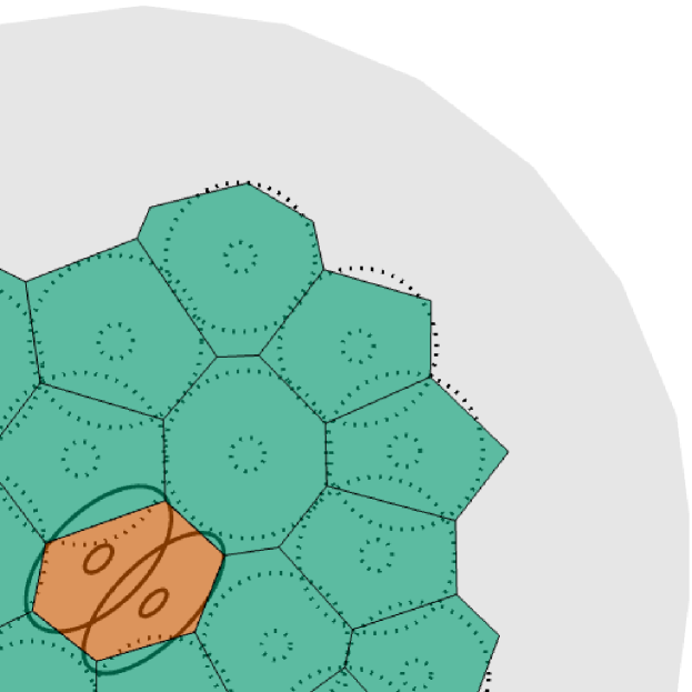
(a)

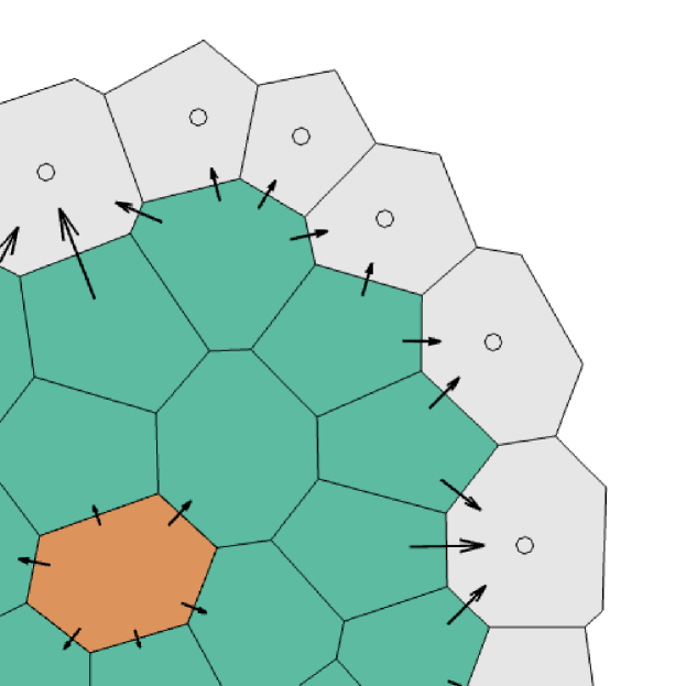
(b)

Figure 2.1: Cell population representation in the DLCM framework using a Voronoi tessellation. Green voxels represent singly occupied voxels and red voxels represent doubly occupied voxels as shown explicitly in Fig. 1(a). The doubly occupied voxels exceed the carrying capacity and exert pressure on the surrounding cells. The movement rates are visualized in Fig. 1(b), where the arrows represent movement rate and direction for a subset of the possible movements. Adapted from [13, Fig. 2.1].

Although the state $u_{i}$ takes on discrete values in each voxel and at any given time, the governing model is derived from a continuous assumptions where the corresponding cell density is then $u=u(x,t)$. We let $u$ be governed by the continuity equation

$$\frac{\partial u}{\partial t}+\nabla\cdot I=0,$$ (2.1)

where $I$ is the advective flux of $u$. There are three main assumptions in the DLCM framework, with the first assumption pointing to the central role of the flux $I$:

Assumption 2.1.

Consider the discrete tissue formed from the populations of cell distributed over the grid. We assume that:

1. The tissue is in mechanical equilibrium when all cells are placed in a voxel of their own.

2. The cellular pressure of the tissue relaxes rapidly to equilibrium in comparison with any other mechanical processes of the system.

3. The cells in a voxel occupied by $n$ cells may only move into a neighboring voxel if it is occupied by less than $n$ cells.

From Assumption 2.1(1) it is clear that random (e.g., Brownian) motion around a voxel center is ignored, and, therefore, that only voxels with cells above the carrying capacity are considered pressure sources. Generally, for the advective flux we have $I=uQ$, where the volumetric flux, $Q$, is determined from the pressure gradient in the form of Darcy’s law which can be derived as a limit for flow through porous media [35]:

$$Q=-D\nabla p,$$ (2.2)

where $p$ is the pressure and the Darcy constant $D$ can be interpreted as the ratio of the medium permeability $\kappa$ to its dynamic viscosity $\mu$, $D:=\kappa/\mu$.

The relation between pressure and cell population is completed by relying on Assumption 2.1(2) to model the pressure according to the stationary heat equation

$$-\Delta p=s(u),$$ (2.3)

where $s(u)$ is the pressure source which then only depends on the voxels above the carrying capacity, (which in the minimal implementation corresponds to $u_{i}>1$ cells).

Finally, we detail the flux parameter $D$ in (2.2). Let $R(e)$ denote the rate of an event $e$, and let $i\rightarrow j$ denote the event that a cell moves from voxel $v_{i}$ to $v_{j}$. With unit carrying capacity only two distinct movements rates are possible according to Assumption 2.1(3): one for cells moving into an empty voxel, and one for cells moving into an already occupied voxel,

$$\left.\begin{array}[]{rcl}R(i\rightarrow j;\quad u_{i}\geq 1,\quad u_{j}=0)&=&u_{i}D_{1}q_{ij}\\ R(i\rightarrow j;\quad u_{i}>1,\quad u_{j}=1)&=&u_{i}D_{2}q_{ij}\end{array}\right\}$$ (2.6)

where $D_{1}$ and $D_{2}$ are (possibly equal) conversion factors from units of pressure gradient to movement rate for the respective case. Here, $q_{ij}$ is the pressure gradient integrated over the boundary shared between the voxels $v_{i}$ and $v_{j}$.

To sum up, a population of cells occupying a grid may be evolved in time by first solving for the pressure in (2.3) using the Laplacian on the grid, and then converting the pressure gradient into rates via (2.2) and (2.6). The rates are now interpreted as competing Poissonian events for the corresponding cellular movements to be simulated as a continuous-time Markov chain. Any other dynamics taking place in continuous time are thus readily incorporated in a consistent way.

2.2 Cell-based stochastic tumor model

As a candidate for a ‘minimal’ avascular tumor model we consider the one presented in [13] which consists of a single cancerous cell type in three different states: proliferating, quiescent (i.e., dormant), and necrotic (i.e., dying) cells. As a matter of convenient implementation the range of $u_{i}$ can be extended to include $u_{i}=-1$ which represents a voxel containing a dead cell so that $u_{i}\in\{-1,0,1,2\}$. Also, let $\Omega$ denote the tumor domain with $u_{i}\neq 0$ and let $\Omega_{\text{ext}}$ denote the entire computational domain.

An avascular tumor has to rely on oxygen and nutrients to diffuse through the surrounding tissue to reach the tumor, readily modeled by the Laplace equation with a boundary condition on the external boundary $\partial\Omega_{\text{ext}}$ (far away from the tumor boundary $\partial\Omega$) as

$$\left.\begin{array}[]{rcl}-\Delta c&=&-\lambda a(u)\\ c&=&c_{\text{out}}\quad\text{ on }\partial\Omega_{\text{ext}}\end{array}\right\}$$ (2.9)

where $c$ is the concentration variable understood as a proxy variable for oxygen and any other nutrients required for the cellular metabolism. Further, $\lambda$ is the rate of consumption for a single cell, and $a(u_{i})$ is the number of living cells in the voxel $i$, i.e., $a(u_{i})=\max(u_{i},0)$. The rates describing the tumor growth are then defined as follows: cells proliferate at rate $\mu_{\text{prol}}$ if $c_{i}\geq\kappa_{\text{prol}}$, where $\kappa_{\text{prol}}$ is the minimum oxygen concentration required for cell proliferation. A cell dies at rate $\mu_{\text{death}}$ if $c_{i}<\kappa_{\text{death}}$, where $\kappa_{\text{death}}$ is the minimum oxygen concentration required for individual cell survival. Finally, dead cells degrade at rate $\mu_{\text{deg}}$ to free up the voxel they are in. Note that cells may switch between all living states provided the oxygen concentration allows for it.

At the tumor boundary a pressure condition needs to be imposed in order to capture the net effect of cell-cell adhesion as well as the interactions between cancerous and healthy cells. We let the phenomenological constant $\sigma$ represent this via a Young-Laplace pressure drop proportional to the boundary curvature $C$. Denoting by $p^{(\text{ext})}$ the ambient pressure outside the tumor (i.e., in $\Omega_{\text{ext}}\setminus\Omega$) we thus have the Dirichlet condition

$$p=p^{(\text{ext})}-\sigma C,\qquad\text{ on }\partial\Omega.$$ (2.10)

A summary of the parameters of the proposed model is found in Tab. 2.1.

Parameter	Description
$D$	Ratio medium permeability to dynamic viscosity $[f^{-1}l^{3}t^{-1}]$
$\lambda$	Rate of oxygen consumption per cell $[t^{-1}l^{-2}]$
$c_{\text{out}}$	Oxygen concentration at oxygen source $[l^{-2}]$
$\mu_{\text{prol}}$	Rate of cell proliferation $[t^{-1}]$
$\mu_{\text{death}}$	Rate of cell death $[t^{-1}]$
$\mu_{\text{deg}}$	Rate of dead cell degradation $[t^{-1}]$
$\kappa_{\text{prol}}$	Oxygen concentration threshold for cell proliferation
$\kappa_{\text{death}}$	Oxygen concentration threshold for cell death
$\sigma$	Surface tension coefficient $[f]$

Table 2.1: Parameters of the cell-based tumor model in two dimensions. The same parameters are used in the corresponding PDE model (except for $\mu_{\text{deg}}$ which is not used) and are nonnegative for both models. The units $t$, $l$, $f$ correspond to units of time, length, and force, respectively.

2.3 Mean-field PDE tumor model

We next derive the corresponding ‘minimal’ partial differential equations (PDE) model, constructed to very closely mimic the mean-field of the stochastic model. While certain aspects of the DLCM model are difficult to interpret in the PDE setting, the underlying continuous physics of the model provide an appropriate starting point for the PDE. The derivation is essentially based on mass balance with a growth- and death rate, and a velocity field proportional to the pressure gradient.

Seeing as cells comprise mostly water we assume that they are incompressible. We begin by considering the conservation law governing tumor cell density $\rho$ in a velocity field $\boldsymbol{v}$

$$\frac{\partial\rho}{\partial t}+\nabla\cdot(\boldsymbol{v}\rho)=\underbrace{\frac{\partial\rho}{\partial t}+\boldsymbol{v}\cdot\nabla\rho}_{=0\text{ by incompressibility}}+\rho\nabla\cdot\boldsymbol{v}=\Gamma,$$ (2.11)

where $\Gamma$ is cell growth and loss due to proliferation or death, respectively, and remains to be defined. Assuming that the cells move as a viscous fluid with low Reynolds number through a porous medium, the velocity field for the cell density is governed by Darcy’s law [35]

$$\boldsymbol{v}=-D\nabla p,$$ (2.12)

where the porous media that the cells reside in is the extra-cellular matrix (ECM), whose permeability is one of two factors determining $D$. Combining (2.11) and (2.12) and assuming a homogeneous permeability within the tissue domain we arrive at

$$-\rho\Delta p=\frac{\Gamma}{D}.$$ (2.13)

For the source term $\Gamma$ we mimic the stochastic model and let the growth and death rates be constant and determined by oxygen thresholds. We thus define $\Gamma$ as

$$\Gamma=\begin{cases}\mu_{\text{prol}}\times\rho&c\geq\kappa_{\text{prol}}\\ 0&\kappa_{\text{death}}\leq c<\kappa_{\text{prol}}\\ -\mu_{\text{death}}\times\rho&c<\kappa_{\text{death}},\end{cases}$$ (2.14)

which defines the proliferative, quiescent, and necrotic region, respectively (see Fig. 2.2). These relations close the pressure relation (2.13).

Similar to the cell-based formulation, we assume a Young-Laplace pressure drop at the outer tumor boundary, which obeys (2.10). This surface tension effect arises from various cell-cell adhesion effects — the loss of which, due to loss of E-cadherin function in cells, is associated with tumor metastasis and tissue invasion [20]. Let $\Omega$ here denote the region with $\rho>0$ akin to the tumor domain of the stochastic model. By Darcy’s law, we then have

$$\diff{\boldsymbol{r}}{t}\cdot\boldsymbol{n}=\boldsymbol{v}\cdot\boldsymbol{n},\qquad\boldsymbol{r}\text{ on }\partial\Omega^{-}(t),$$ (2.15)

where $\boldsymbol{n}$ is the interface normal vector and $\partial\Omega^{-}(t)$ denotes the boundary as approached from inside $\Omega$. The condition (2.15) connects the velocity field with the movement of the tumor boundary.

figurec

Figure 2.2: Schematic of circular tumor with three distinct regions. Arrows show the distinct radii, $r_{p}$, $r_{q}$, and $r_{n}$ which correspond to the distance from the origin to respective regional interface.

The pressure boundary conditions concern the external medium that the tumor grows within. Recall that $\Omega_{\text{ext}}$ is the domain containing both $\Omega$ and the external medium. By assuming that the external medium obeys laws similar to the tumor tissue, we can summarize the medium’s impact on the tumor growth through the tumor boundary conditions. We start from the assumption that the pressure propagates freely throughout the external medium outside the tumor and, for consistency of the complete two-tissue system, the external medium is assumed to abide by the same assumptions as the tumor tissue (i.e., incompressibility, Darcy’s law, and conservation of mass). We further assume that growth and death of the external tissue is negligible and, thus, arrive at the governing equation for the outer pressure, $p^{(\text{ext})}$ in $\Omega_{\text{ext}}\setminus\Omega$:

$$\Delta p^{(\text{ext})}(\boldsymbol{r}) = 0,$$ (2.16)

where the solution is undetermined up to a specified boundary condition. The velocities of the tumor and the external tissue are both determined by Darcy’s law, but are allowed different Darcy coefficients, $D$ and $D_{\text{ext}}$, respectively. The velocities are assumed compatible at the interface and the complete set of boundary conditions on $\partial\Omega$ thus reads as

$$p =p^{(\text{ext})}-\sigma C,$$ (2.17)

$$\boldsymbol{n}\cdot D\nabla p =\boldsymbol{n}\cdot D_{\text{ext}}\nabla p^{(\text{ext})},$$ (2.18)

where $\boldsymbol{n}$ is the interface normal vector. Thus, we assume that the physical extent of the region between the tissues (where cell mixing might occur) is negligible in comparison with the spatial scale of the model. The nondimensional coefficient is expressed as $\hat{D}_{\text{ext}}=D_{\text{ext}}/D$, but for brevity we omit the hat in the following analysis. The compatibility condition (2.18) allows for an investigation into the effects of varying the stiffness between the tumor and the external tissue due to, e.g., an increase in collagen density [33]. For simplicity, we assume that the ECM permeability is homogeneous and time-independent across the domain of tissues, hence implicitly assuming that breakdown and remodeling of ECM that could affect tumor progression [26] are negligible.

Finally, oxygen diffuses in towards the tumor through the surrounding tissue from a source (e.g., a vessel) far away with regards to the spatial scale of the system. Akin to the cell-based model, oxygen diffusion occurs on a shorter timescale than cell growth and migration. Thus, the oxygen concentration $c$ satisfies (2.9) with source term

$$-\Delta c=\begin{cases}-\lambda\rho, \quad&c\geq\kappa_{\text{death}}\\ 0, \quad&c<\kappa_{\text{death}}\text{ on }\Omega_{\text{ext}}\end{cases}\\$$ (2.19)

with $c=c_{\text{out}}$ on $\partial\Omega_{\text{ext}}$ and where $\lambda$ is consumption rate per cell density in the PDE setting. We assume that $\partial\Omega_{\text{ext}}$ is radially symmetric and lies at a distance $R$ from the domain origin and we also make the simplifying assumption that the external tissue consumes negligible oxygen.

A suitable choice for the characteristic length is $l_{c}=R$ as it remains constant during growth. Nondimensionalization of the model assuming a radially symmetric tumor then yields the characteristic units

$$l_{c}=R,\quad v_{c}=\mu_{\text{prol}}R,\quad t_{c}=1/\mu_{\text{prol}},\quad p_{c}=\mu_{\text{prol}}R^{2}/D,$$ (2.20)

with the dimensionless parameters $\hat{\sigma}=D/(\mu_{\text{prol}}R^{3})\times\sigma$ and $\hat{\mu}_{\text{death}}=\mu_{\text{death}}/\mu_{\text{prol}}$. We nondimensionalize the oxygen parameters independently of the pressure and arrive at the characteristic units and additional dimensionless parameter, respectively, as

$$\left.\begin{array}[]{l}\quad c_{c}=c_{\text{out}},\quad\hat{\lambda}=R^{2}\lambda/c_{\text{out}},\\ \hat{\kappa}_{\text{prol}}=\kappa_{\text{prol}}/c_{\text{out}},\quad\hat{\kappa}_{\text{death}}=\kappa_{\text{death}}/c_{\text{out}}.\end{array}\right\}$$ (2.23)

Subsequently, we use the characteristic units and nondimensional parameters, but we drop the hats. The units are set to one such that $R=1$, $\mu_{\text{prol}}=1$, $c_{\text{out}}=1$, and $D=1$.

While the PDE model is intended to closely match the mean-field of the DLCM model, we anticipate certain differences between the two and view the PDE model as an effective model of the DLCM model. For the simulation of the PDE model, we thus use effective parameters that we derive from the outcome of the DLCM simulations (details in §4).

3 Analysis

We analyze the morphological properties of the tumor model in two spatial dimensions. This simplifies the analysis while formally still allowing for a comparison with in vitro data from flat two-dimensional cell cultures. The case of a radially symmetric growth is discussed in §3.1 and a spatial linear stability analysis in §3.2. In essence, the outcome of the latter analysis include conditions for when the former radially symmetric case is a valid ansatz. Finally, in §3.3 we uncover how the morphological instabilities of the model develop during its different growth phases and a possible role of the external medium in exacerbating or reducing such effects.

3.1 Radial symmetry and the stationary state

A characteristic property of the avascular tumor is that it reaches a stationary growth phase due to limited oxygen/nutrition availability [15]. We therefore first derive analytical relations that provide insight into which regions of our model’s parameter space map to such a stationary state under the preliminary assumption that the tumor is radially symmetric.

The constant growth and death rates of cells define distinct characteristic regions of the model tumor according to (2.14): the proliferative, quiescent, and necrotic region. For a radially symmetric tumor at time $t\geq 0$, motivated by the form of the oxygen field governed by (2.19), we let $r_{p}(t)$ denote the tumor radius, $r_{q}(t)$ the radius of the interface between the proliferative and quiescent region, and $r_{n}(t)$ the radius of the interface between the quiescent and necrotic region, cf. Fig. 2.2. Given $\lambda>0$, the assumed radial symmetry implies that $0\leq r_{n}\leq r_{q}\leq r_{p}$, and under the chosen units, $r_{p}<R=1$. We note that if $r_{p}$ is sufficiently close to the oxygen source at $R$, the model assumption of avascularity breaks down.

We simplify the problem by assuming that $\rho=1$ across the entire tumor domain since this allows the oxygen field to be explicitly solved. By incompressibility and slow migration of cells, this is a reasonable approximation and, besides, a constant cell density in the PDE model is a close match to the discrete stochastic model that we wish to investigate.

We thus solve (2.19) under radial symmetry while imposing $C^{1}$-continuity for the oxygen $c$ across the interfaces between the characteristic regions. Under radial symmetry, the divergence theorem implies an inhomogeneous Neumann boundary condition across each radial boundary whose value is proportional to the volume of oxygen sinks contained within. We find the full solution to (2.19) in two-dimensional space:

$$c(r) =\left\{\begin{array}[]{ll}1+\lambda/2\,\left(r_{p}^{2}-r_{n}^{2}\right)\log r,&r_{p}\leq r,\\ 1+\lambda/2\,\left(r_{p}^{2}\log r_{p}-r_{n}^{2}\log r+(r^{2}-r_{p}^{2})/2\right),&r_{n}\leq r\leq r_{p},\\ \kappa_{\text{death}},&r\leq r_{n},\end{array}\right.$$ (3.4)

where the expression does not differ in the proliferative and quiescent regions since the oxygen consumption rates are identical there. By definition, the oxygen level at $r_{q}$ is $\kappa_{\text{prol}}$ and at $r_{n}$ it is $\kappa_{\text{death}}$. Using this, (3.4) implies the following algebraic relations between the characteristic regions

$$\left.\begin{array}[]{rclcl}K_{\text{prol}}&:=&4(1-\kappa_{\text{prol}})/\lambda&=&-r_{p}^{2}\log r_{p}^{2}+r_{n}^{2}\log r_{q}^{2}-r_{q}^{2}+r_{p}^{2}\\ K_{\text{death}}&:=&4(1-\kappa_{\text{death}})/\lambda&=&-r_{p}^{2}\log r_{p}^{2}+r_{n}^{2}\log r_{n}^{2}-r_{n}^{2}+r_{p}^{2}\end{array}\right\}$$ (3.7)

in terms of the reduced parameter set $\{K_{\text{prol}},K_{\text{death}}\}$.

Given radial symmetry and $\rho=1$, the tumor volume change is derived from mass balance as $\dot{V}=\mu_{\text{prol}}V_{p}-\mu_{\text{death}}V_{n}$, where $V_{p}$ and $V_{n}$ are the volumes of the proliferative and necrotic region, respectively. Thus, in two spatial dimensions we get that

$$d/dt\,\left(r_{p}^{2}\right)=-\mu_{\text{death}}r_{n}^{2}-r_{q}^{2}+r_{p}^{2},$$ (3.8)

under the nondimensionalization where $\mu_{\text{prol}}=1$.

Assume now that $(r_{n}^{\text{eq}},r_{q}^{\text{eq}},r_{p}^{\text{eq}})$ is a stationary solution of (3.7)–(3.8). By implicit differentiation we can linearize (3.8) around this solution and retrieve the single eigenvalue

$$\Lambda_{r} =1-\frac{\log r_{p}^{\text{eq}}}{\log r_{n}^{\text{eq}}}\left(\mu_{\text{death}}+\frac{2\log\frac{r_{q}^{\text{eq}}}{r_{n}^{\text{eq}}}}{(r_{q}^{\text{eq}})^{2}-(r_{n}^{\text{eq}})^{2}}\,(r_{q}^{\text{eq}})^{2}\right).$$ (3.9)

Proposition 3.1 (Stability of radially symmetric equilibrium).

Given $\mu_{\text{death}}>0$, assume that $0\leq r_{n}^{\text{eq}}\leq r_{q}^{\text{eq}}\leq r_{p}^{\text{eq}}$ is a stationary solution of (3.7)–(3.8). Then $\Lambda_{r}<0$ in (3.9) whenever $r_{p}^{\text{eq}}\leq\exp(-1)\approx 0.368$.

Proof.

Put $(r_{n}^{\text{eq}})^{2}=\theta(r_{q}^{\text{eq}})^{2}$ for some $\theta\in(0,1)$ and note that $(r_{p}^{\text{eq}})^{2}=(1+\mu_{\text{death}}\theta)(r_{q}^{\text{eq}})^{2}$ by stationarity (the cases $\theta\in\{0,1\}$ are treated as limits). The eigenvalue becomes

$$\Lambda_{r} =1-\frac{\log r_{p}^{\text{eq}}}{\log r_{p}^{\text{eq}}+\frac{1}{2}\log\left(\theta/(1+\mu_{\text{death}}\theta)\right)}\left(\mu_{\text{death}}-\frac{\log\theta}{1-\theta}\right).$$

By inspection we find that as a function of $\mu_{\text{death}}$, the expression on the right is monotonically decreasing and hence it is bounded by its behavior as $\mu_{\text{death}}\to 0+$:

$$\Lambda_{r} <1+\frac{\log r_{p}^{\text{eq}}}{\log r_{p}^{\text{eq}}+\frac{1}{2}\log\theta}\times\frac{\log\theta}{1-\theta}.$$

In turn, as a function of $r_{p}^{\text{eq}}$, this expression is monotonically increasing such that, in particular, for $r_{p}^{\text{eq}}\leq\exp(-1)$ we have that

$$\Lambda_{r} <1+\frac{\log\theta}{1-\frac{1}{2}\log\theta}\times\frac{1}{1-\theta}.$$

From the elementary inequality $-y\leq(\exp(-y)-1)\cdot(1+y/2)$ for $y\geq 0$ we finally conclude, taking $y=-\log\theta$, that $\Lambda_{r}<0$. ∎

Proposition 3.1 can be thought of as a modeling cut-off: either a radially symmetric tumor is small enough to be stable, or it has grown too large relative to the oxygen source for stability to be guaranteed and can therefore no longer be considered avascular. In the numerical experiments in §4, we use Proposition 3.1 to ensure that the tumor is small enough that a radially symmetric solution is expected to reach a stable stationary state. For suggested stationary radii $(r_{n}^{\text{eq}},r_{q}^{\text{eq}},r_{p}^{\text{eq}})$, with $r_{p}^{\text{eq}}$ small enough, $\mu_{\text{death}}$ is defined by setting (3.8) to 0, and similarly $K_{\text{prol}}$ and $K_{\text{death}}$ are found from (3.7).

3.2 Morphological stability

We analyze the stability of the PDE model by studying the system’s response to perturbations of a radially symmetric solution. The main result depends on the three Lemmas in §A and reads as follows:

Theorem 3.2 (Linear stability).

Let the outer tumor boundary $r_{p}$ be perturbed by

$$\tilde{r}_{p}(\theta)=r_{p}+\epsilon\sum_{k=1}^{\infty}\alpha_{k}^{(p)}\cos(k\theta),$$ (3.10)

for some $\lvert\epsilon\rvert\ll 1$. Write the induced inner perturbations on the same form,

$$\begin{split}\tilde{r}_{q}(\theta)&=r_{q}+\epsilon\sum_{k=1}^{\infty}\alpha_{k}^{(q)}\cos(k\theta),\\ \tilde{r}_{n}(\theta)&=r_{n}+\epsilon\sum_{k=1}^{\infty}\alpha_{k}^{(n)}\cos(k\theta),\end{split}$$ (3.11)

each defined as the interface between the regions of different growth rates according to (2.14) with the oxygen field governed by (2.19) (see also Fig. 2.2). We let the pressure field and the cell density advection be defined as in §2.3. Let the $k$th perturbation mode in (3.10) grow as $\alpha_{k}^{(p)}(t)\propto e^{\Lambda(k)t}$. Then, to first order in $\epsilon$,

$$\Lambda(k) =\frac{r_{p}^{\prime}}{r_{p}}\Biggl{(}\overbrace{\frac{1-D_{\text{ext}}}{1+D_{\text{ext}}}k}^{\text{Saffman-Taylor}}-1\Biggr{)}$$ (3.12)

$$+ \frac{D_{\text{ext}}}{1+D_{\text{ext}}}\Biggl{(}1-\underbrace{r_{p}^{-k-1}\left(\mu_{\text{death}}r_{n}^{k+1}\frac{\alpha_{k}^{(n)}}{\alpha_{k}^{(p)}}+r_{q}^{k+1}\frac{\alpha_{k}^{(q)}}{\alpha_{k}^{(p)}}\right)}_{\text{inner region perturbation}}-\underbrace{\sigma\frac{k(k^{2}-1)}{r_{p}^{3}}}_{\text{surface tension}}\Biggr{)},$$

in which the interface perturbation coefficients $\alpha_{k}^{(q)}$, $\alpha_{k}^{(n)}$ are given by (A.11) and where the radial growth follows from (3.8),

$$r_{p}^{\prime} =-\frac{1}{2r_{p}}(\mu_{\text{death}}r_{n}^{2}+r_{q}^{2}-r_{p}^{2})=-p{{}^{\prime}}(r_{p}),$$ (3.13)

by Darcy’s law.

Proof.

We first solve for the pressure field (2.13) under the assumption of radial symmetry where, again, the divergence theorem implies Neumann interface conditions. The result is

$$p^{(\text{ext})}(r) =(\mu_{\text{death}}r_{n}^{2}+r_{q}^{2}-r_{p}^{2})\frac{1}{2D_{\text{ext}}}\log(r), \quad r_{p}\leq r$$ , (3.14)

$$p^{(p)}(r) =(\mu_{\text{death}}r_{n}^{2}+r_{q}^{2})\frac{1}{2}\log\frac{r}{r_{p}}-\frac{1}{4}(r^{2}-r_{p}^{2})+p^{(\text{ext})}(r_{p})-\sigma C, \quad r_{q}\leq r \leq r_{p},$$ (3.15)

$$p^{(q)}(r) =p^{(p)}(r_{q})+\frac{1}{2}r_{n}^{2}\log\frac{r}{r_{q}}, \quad r_{n}\leq r \leq r_{q},$$

$$p^{(n)}(r) =p^{(q)}(r_{n})+\frac{\mu_{\text{death}}}{4}(r^{2}-r_{n}^{2}), \quad 0\leq r \leq r_{n},$$ (3.16)

where the negative pressure gradient at $r_{p}$ (3.15) recovers the velocity of the tumor’s outer rim (3.8) as expected.

We continue by perturbing the tumor boundary according to (3.10) using the ansatz $\alpha_{k}^{(p)}=\alpha_{k}^{(p)}(t)\propto e^{\Lambda(k)t}$. Similarly, we let the induced pressure perturbation in each region $i\in\{\text{ext},p,q,n\}$ be

$$\tilde{p}^{(i)}(r) =p^{(i)}(r)+\epsilon\sum_{k=1}^{\infty}\gamma_{k}^{(i)}(r)\cos(k\theta).$$

Using similar arguments to those in the proof of Lemma A.3, we can show that the pressure perturbation coefficients are on the form (A.13). We next use Lemmas A.1 and A.2 to find the continuity relations for the coefficients. However, the pressure discontinuity at the tumor boundary, (2.17) and (2.18), must be treated separately. For the former, the first order approximation in $\epsilon$ of $\sigma C(r_{p}^{*})$ is evaluated, and for the latter we use that $D$ and $D_{\text{ext}}$ are constant within their respective domains. Thus, the continuity relations become

$$\begin{split}\gamma_{k}^{(p)}(r_{p})&=\gamma_{k}^{(\text{ext})}(r_{p})+(p^{(\text{ext})}{{}^{\prime}}(r_{p})-p{{}^{\prime}}(r_{p})+\sigma\frac{k^{2}-1}{r_{p}^{2}})\alpha_{k}^{(p)},\\ \gamma_{k}^{(p)}(r_{q})&=\gamma_{k}^{(q)}(r_{q}),\\ \gamma_{k}^{(q)}(r_{n})&=\gamma_{k}^{(n)}(r_{n}),\end{split}$$

and for the derivatives,

$$\begin{split}\gamma_{k}^{(p)}{{}^{\prime}}(r_{p})&=-p{{}^{\prime\prime}}(r_{p})\alpha_{k}^{(p)}+D_{\text{ext}}(\gamma_{k}^{(\text{ext})}{{}^{\prime}}(r_{p})+p^{(\text{ext})}{{}^{\prime\prime}}(r_{p})\alpha_{k}^{(p)}),\\ \gamma_{k}^{(p)}{{}^{\prime}}(r_{q})&=\gamma_{k}^{(q)}{{}^{\prime}}(r_{q})+\alpha_{k}^{(q)}(p^{(p)}{{}^{\prime\prime}}(r_{q})-p^{(q)}{{}^{\prime\prime}}(r_{q})),\\ \gamma_{k}^{(q)}{{}^{\prime}}(r_{n})&=\gamma_{k}^{(n)}{{}^{\prime}}(r_{n})+\alpha_{k}^{(n)}(p^{(q)}{{}^{\prime\prime}}(r_{n})-p^{(n)}{{}^{\prime\prime}}(r_{n})).\\ \end{split}$$

As in [17], we find the form of this dispersion relation from the velocity at the tumor boundary by applying (2.12) to (2.15) for the perturbed solution. Considering only the first order terms in $\epsilon$, we get

$$\Lambda(k)=-\left(p{{}^{\prime\prime}}(r_{p})+\frac{\gamma_{k}^{(p)}{{}^{\prime}}(r_{p})}{\alpha_{k}^{(p)}}\right).$$ (3.17)

Finally, evaluating (3.17) using Lemma A.3 for the coefficients $\alpha_{k}^{(q)}$, $\alpha_{k}^{(n)}$ yields the dispersion relation (3.12). ∎

Note that (3.12) is independent of the coefficients $\alpha_{k}^{(p)}$ of the initiating perturbation since both $\alpha_{k}^{(n)}$ and $\alpha_{k}^{(q)}$ are proportional to $\alpha_{k}^{(p)}$, as seen in (A.11). It follows that $\Lambda(k)$ is unambiguously determined by the set of parameters and values $\{r_{p},r_{q},r_{n},\mu_{\text{death}},D_{\text{ext}},\sigma\}$.

The first part in (3.12) is the Saffman-Taylor instability [29] term. This type of instability has previously been discussed in the context of growing cell populations [24]. Further, the induced perturbations on the oxygen field act to dampen any morphological instability as seen by the inner region perturbation term, which is negative and can only decrease the value of $\Lambda(k)$. However, for large $k$ this dampening vanishes in general as is seen from the following reasoning. Let $r_{n}^{2}=\theta_{n}r_{p}^{2}$, $r_{q}^{2}=\theta_{q}r_{p}^{2}$, with $0\leq\theta_{n}<\theta_{q}<1$, i.e., the regions do not overlap. Then the inner region perturbation term becomes

$$\frac{1-r_{p}^{2k}}{1-\theta_{n}^{k}r_{p}^{2k}}\left(\mu_{\text{death}}\theta_{n}^{k}+\frac{\theta_{q}^{k}-\theta_{n}^{k}}{\theta_{q}-\theta_{n}}\times\frac{1}{k}\times\theta_{q}\right),$$ (3.18)

which for $r_{p}<1$ tends to zero as $k$ grows. Finally, surface tension also reduces the amplitude and range of unstable perturbation modes. Similar effects are observed due to cell adhesion in glioblastoma models in silico and in vitro [25].

3.3 Notable special cases

The dispersion relation (3.12) provides rich insight into the morphological dynamics of our model of a growing avascular tumor. We outline notable regimes of these dynamics below.

The Saffman-Taylor instability

When the tumor grows in a medium that flows on a significantly smaller timescale than the tumor itself, corresponding to $D_{\text{ext}}\gg D$ ($\equiv 1$ by nondimensionalization), the dispersion relation becomes

$$\Lambda(k) =-\frac{r_{p}^{\prime}}{r_{p}}(k+1)$$ (3.19)

$$\phantom{=}+1-r_{p}^{-k-1}\left(\mu_{\text{death}}r_{n}^{k+1}\frac{\alpha_{k}^{(n)}}{\alpha_{k}^{(p)}}+r_{q}^{k+1}\frac{\alpha_{k}^{(q)}}{\alpha_{k}^{(p)}}\right)-\sigma\frac{k(k^{2}-1)}{r_{p}^{3}}.$$

One can show that the same equations are obtained by assuming a homogeneous outer pressure, $p^{(\text{ext})}(r)=p_{0}$, for some constant $p_{0}$. The Saffman-Taylor term (the first term) is here at its most stabilizing since $k(1-D_{\text{ext}})/(1+D_{\text{ext}})\geq-k$ for $D_{\text{ext}}\geq 0$. On the other side of the spectrum, we have the situation when the external tissue is significantly more viscous and practically immovable within the temporal scale of the growing tumor. This corresponds to the condition $D_{\text{ext}}\ll 1$, and (3.12) becomes

$$\Lambda(k) = \frac{r_{p}^{\prime}}{r_{p}}(k-1),$$ (3.20)

and every mode $k\geq 2$ is unstable during growth with no stabilizing effect from the surface tension. The case $D_{\text{ext}}<1$ is the common form of the Saffman-Taylor instability.

Growth phases

The tumor’s morphological stability depends on which growth phase the tumor is in. We identify the following quantity as a discriminant of the tumor’s growth phase:

$$\Delta_{\theta}=\frac{r_{p}^{\prime}}{r_{p}},$$ (3.21)

i.e., the relative tumor boundary velocity. When the tumor is initially growing in a nutrient-rich environment, and $r_{n}$, $r_{q}$ are small, then $\Delta_{\theta}\approx\frac{1}{2}$ and (3.12) becomes

$$\Lambda(k)=\frac{1-D_{\text{ext}}}{2(1+D_{\text{ext}})}(k-1)-\frac{D_{\text{ext}}}{1+D_{\text{ext}}}\sigma\frac{k(k^{2}-1))}{r_{p}^{3}}.$$ (3.22)

Hence as the tumor grows exponentially, we expect all modes $k>1$ to be stable for $D_{\text{ext}}>1$ and unstable for $D_{\text{ext}}<1$ in the absence of surface tension effects.

As the tumor grows larger and the nutrient availability can no longer sustain the entire tumor, the tumor front slows down and $\Delta_{\theta}\rightarrow 0^{+}$, and the effect from the Saffman-Taylor part diminishes. From (3.18) we see that the inner region perturbation term in (3.12) is negative, and hence close to the tumor’s stationary state we have that

$$\Lambda(k)<\frac{D_{\text{ext}}}{1+D_{\text{ext}}}\Bigl{(}1-\sigma\frac{k(k^{2}-1)}{r_{p}^{3}}\Bigr{)},$$ (3.23)

Since the inner region perturbation term tends to zero for increasing $k$, the upper bound becomes a good approximation of $\Lambda(k)$ for large $k$. Clearly, (3.23) shows that a positive value of $\sigma$ is necessary for the stationary stability.

Surface tension and stationarity

The stability relation provides an estimate of the surface tension required to maintain a radially symmetric growth as $t\rightarrow\infty$. Considering only the case when $D_{\text{ext}}\gg 1$, we see from (3.19) that the least stable case with respect to the discriminant is obtained when $\Delta_{\theta}=0$. We find the necessary surface tension by requiring $\Lambda(k)=0$ for all $k$. Again, using that the inner region perturbation term is negative, we obtain from (3.19) the bound

$$\sigma_{\text{stable},k}\leq\frac{r_{p}^{3}}{k(k^{2}-1)}$$ (3.24)

where $\sigma_{\text{stable},k}$ is the lower bound of $\sigma$ required for stabilizing small perturbations of mode $k$. Thus, to stabilize all modes $k\geq 2$ it is sufficient to have that $\sigma=r_{p}^{3}/6$, depending only on the total tumor volume. Again, since the inner perturbation term tends to zero as $k$ grows, the upper bound is a good approximation of $\sigma_{\text{stable},k}$ for large $k$.

Creeping instability

We finally remark on the interesting mode $k=1$, the only mode unaffected by surface tension. Geometrically, this mode corresponds to movement of the tumor’s center of mass: the tumor begins to creep towards the oxygen source given a small perturbation. From (3.12),

$$\Lambda(k=1)=\frac{D_{\text{ext}}}{1+D_{\text{ext}}}\frac{\mu_{\text{death}}r_{n}^{2}+r_{q}^{2}}{r_{p}^{2}}\times\frac{r_{p}^{2}-r_{n}^{2}}{1-r_{n}^{2}}\geq 0.$$ (3.25)

Thus, the tendency for creeping always exists when $r_{q}$ and/or $r_{n}$ are positive, and the model would require additional features regarding, e.g., the external tissue’s response to invasion, in order to inhibit this effect. Note that this tendency is reduced for tumors growing within an environment more viscous and/or less permeable than its own. As showed previously, however, such conditions make all the other modes $k\geq 2$ less stable.

4 Numerical examples

In the following section, we present numerical simulations of both the stochastic model from §2.2 and the PDE model from §2.3. We focus on the case $D_{\text{ext}}\gg 1$ which we showed had an inherent stabilizing effect during growth in §3.3. In §4.1 we assess the validity of the assumption that growth is radially symmetric and how the stability responds to surface tension. In §4.2, we explore the relation between surface tension and the emergent morphology and compare the outcomes between the stochastic and the mean-field PDE model.

Due to certain differences between the models, we use effective parameter values for the PDE simulations for the parameters $\mu_{\text{prol}}$, $\mu_{\text{death}}$ and $\lambda$, and denote those with a bar, e.g., $\bar{\mu}_{\text{prol}}$. The effective parameters are derived from the stochastic model simulations via basic scaling considerations or preliminary simulations. First, due to doubly occupied voxels consuming twice the amount of oxygen in DLCM, the effective $\lambda$ can be expected to be greater for the corresponding PDE assuming identical characteristic regions. The effective parameters $\bar{\mu}_{\text{death}}$ and $\bar{\lambda}$ are found using (3.7) and (3.8), respectively, and taking the mean over the stationary state of the DLCM simulation. Second, we expect a difference in volumetric growth rates between the models since the DLCM tumor must undergo both a proliferation event and a migration event separately to expand in size. From studying the DLCM volume growth during the exponential growth phase, we find that $\bar{\mu}_{\text{prol}}=\mu_{\text{prol}}/2.5$ is a good approximation that makes respective tumor evolution comparable.

The set of parameters used in both the DLCM and the PDE simulations are found in Tab. 4.1.

Parameter	Value
$\mu_{\text{death}}$	0.5 (1.35)
$\mu_{\text{deg}}$	0.05 (N/A)
$\kappa_{\text{prol}}$	0.94
$\kappa_{\text{death}}$	0.93
$\lambda$	1 (1.15)
$p^{(\text{ext})}$	0
$D_{\text{ext}}$	$+\infty$
$D_{2}$	25 (N/A)

Table 4.1: Standard set of parameters of the DLCM model with effective parameter values used for the PDE in parenthesis. No parenthesis means that the models use the same parameters.

4.1 Radial symmetry and surface tension

We first solve the PDE under the assumption of radial symmetry. We solve the reduced 1D problem comprising (3.7) and (3.8) as derived in §3.1 and evaluate the perturbation growth factors (3.19) during tumor growth and study their response to surface tension. For quantitative measurements of the regional characteristics during tumor growth, we consider the volumetric quantities $V_{p}=\pi r_{p}^{2}$, $V_{q}=\pi r_{q}^{2}$, and $V_{n}=\pi r_{n}^{2}$.

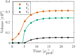
(a)

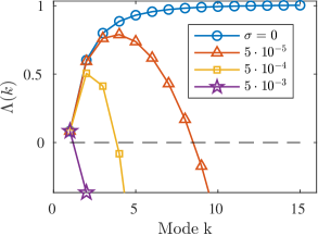
(b)

Figure 4.1: Regional characteristics and perturbation growth factors under the assumption of radial symmetry. Fig. 1(a) shows the evolution of the three characteristic regions. Fig. 1(b) shows the perturbation growth factors (3.19) for the first few modes at the tumor’s stationary state and at varying surface tension $\sigma$.

Fig. 4.1 shows the evolution of the regional characteristics for a simulation using the standard parameters for the PDE found in Tab. 4.1, accompanied by the perturbation growth factors (3.19) at the stationary state. In Fig. 1(a) we observe the emergence of the characteristic sigmoidal growth of the total volume, with an initially exponential growth followed by a growth rate that plateaus. Fig. 1(b) shows the perturbation growth factors versus mode close to the stationary state for a range of $\sigma$. It is clear that the assumption of radial symmetry for low values of $\sigma$ does not hold when oxygen is not sufficient to sustain the growth of the entire population. From (3.19) we find that $\sigma_{\text{stable},2}\approx 3.1\cdot 10^{-3}$, i.e., this is the value needed to stabilize modes $k\geq 2$. From Fig. 1(b) we see that $\sigma$ lower than this prompt nontrivial spatial behavior with instabilities that may occur over different timescales (investigated further in §4.2).

(a)

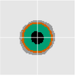
(b)

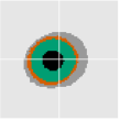
(c)

Figure 4.2: Solution using a surface tension large enough to ensure stability and hence radial symmetry, $\sigma=3.2\cdot 10^{-3}$. Times $t=0.1$, $t=10$, $t=80$, respectively, from left to right. Red: proliferative cells, green: quiescent cells, black: necrotic cells, dark grey: previously occupied. The white cross-hairs are centered on the domain origin.

As suggested by (3.25), creeping is expected for long enough times. We test this in Fig. 4.2, where we simulate the model using $\sigma=3.2\cdot 10^{-3}$ to ensure that modes $k\geq 2$ are stabilized. The tumor reaches close to its stationary state at around $t=10$, in accordance with the solution to the 1D equations in Fig. 4.1. We observe a notable collective migration from the domain origin starting at $t=80$.

4.2 The emergent morphology and its response to stochasticity

We compare the morphology and the growth patterns of the stochastic model and the PDE model for similar parameters. We add some white noise to the cell density updates of the PDE solution to ensure an even distribution of induced boundary perturbations (details found in §B). We evaluate the tumor boundary roundness defined over a 2D region as

$$\text{Roundness}=\frac{4\pi\times\text{Area}}{\text{Perimeter}^{2}},$$ (4.1)

which ranges from $0$ to $1$, where $1$ means the shape is perfectly circular and smaller values measure its deviation from circularity.

We first investigate numerically the effects of surface tension on the tumor morphology. Specifically, we study the onset of second mode instability according to (3.19) for a tumor growing in two spatial dimensions. For this purpose, we compare the growth using $\sigma=2\cdot 10^{-3}$ and $\sigma=5\cdot 10^{-4}$ until $t=30$, during which the former value is stable for $k=2$ although it is not stable over larger times $t$.

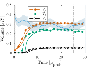
(a)

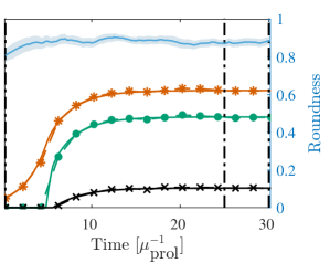
(b)

Figure 4.3: Evolution of characteristic volumes for DLCM (left) and PDE (right), respectively, using the standard parameters in Tab. 4.1 and $\sigma=2\cdot 10^{-3}$. The numerical solutions are compared with the 1D solution using the same parameters. Blue shows the roundness (4.1) of the tumor boundary over time with moving standard deviation shaded. The dashed vertical lines indicate the times $t=0$, $25$, $30$ of the solutions shown in Fig. 4.4.

(a)

(b)

(c)

(d)

(e)

(f)

Figure 4.4: Solutions corresponding to Fig. 4.3 with DLCM in the top row and the PDE in the bottom row. Color scheme as in Fig. 4.2. For DLCM darker gray shows quiescent cells below $\kappa_{\text{death}}$, and darker shades of red and green indicate doubly occupied voxels.

Fig. 4.3 shows the evolution of the tumor’s characteristic volumes for both models together with the tumor roundness (4.1) using the larger value of $\sigma$. Fig. 4.4 shows snapshots of the solution corresponding to Fig. 4.3. Both solutions remain close to being radially symmetric during the full simulations since the small second mode instability does not show during these relatively short time intervals. Notably, the creeping effect becomes apparent earlier for the DLCM simulations.

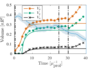
(a)

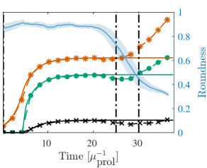
(b)

Figure 4.5: Evolution of characteristic volumes for DLCM (left) and PDE (right), respectively, using the standard parameters Tab. 4.1 and $\sigma=5\cdot 10^{-4}$, which is insufficient to ensure radial symmetry. The numerical solution volumes are compared with the 1D solution volumes using the same parameters and shown in the same units of time. The PDE model tumor splits into two parts just before the final time where the roundness metric is undefined. The dashed vertical lines indicate the times $0,25,30$ of the spatial solutions shown in Fig. 4.6.

(a)

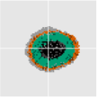
(b)

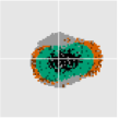
(c)

(d)

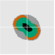
(e)

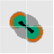
(f)

Figure 4.6: Solutions corresponding to Fig. 4.5. Color scheme as in Fig. 4.4

Similarly, Fig. 4.5 and Fig. 4.6 shows regional evolution and spatial solutions, respectively, for the lower value of $\sigma$. Both models display a significant decrease in roundness (accompanied by a total volume increase) as the tumor begins to split in two some time after the growth has plateaued. A notable difference between the growth curves during this process is that the DLCM tumor does not reach a fully stationary state before the splitting, possibly due to the higher exposure to noise in the stochastic model.

Finally, 4.7 shows the resulting morphology of both models using four different and smaller values of $\sigma$. For these experiments we use use a lower $\kappa_{\text{death}}=0.92$ for a thinner proliferating rim which results in effective parameters $\bar{\mu}_{\text{death}}=1.0$ and $\bar{\lambda}=1.1$. Again, the radially symmetric tumor displays a significant creeping only for the DLCM model at the selected final time (cf. Fig. 7(a) and Fig. 7(e)). The morphologies of the tumors are similar in terms of emergent unstable modes and sizes of the characteristic regions. For the most unstable case using $\sigma=0$ in Fig. 7(d), the DLCM tumor grows somewhat larger and with different morphological and regional characteristics. Finally, Fig. 7(a) and Fig. 7(c) displays small cell clusters detaching from the tumor to grow on their own, a phenomena that we never observe in our simulations of the PDE model.

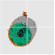
(a)

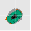
(b)

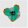
(c)

(d)

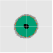
(e)

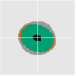
(f)

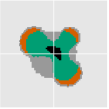
(g)

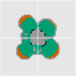
(h)

Figure 4.7: Solutions to DLCM (top row) and the PDE (bottom row) for various parameters highlighting different aspects of the model in relation to (3.12). Left to right shows decreasing surface tension with $\sigma=2\cdot 10^{-3}$, $7\cdot 10^{-4}$, $1\cdot 10^{-4}$, $0$, and top row uses parameters $\kappa_{\text{prol}}=0.94$, $\kappa_{\text{death}}=0.92$, $\mu_{\text{death}}=0.5$, with bottom row using effective parameters $\bar{\mu}_{\text{death}}=1.0$, $\bar{\lambda}=1.1$. Solutions are shown at $t=30$. Color scheme as in Fig. 4.4

5 Discussion

We have analyzed the morphological stability of a PDE model of avascular tumors. The PDE was derived to closely represent the mean-field of a stochastic model expressed in the DLCM framework. Assuming radial symmetry in the PDE model, we first characterized the growth dynamics as well as the stationary state. A linear stability analysis in two dimensions was subsequently carried out and we found a dispersion relation that describes the stability of the morphology of the tumor. Finally, we compared the analytical predictions with numerical simulations of both the stochastic DLCM and the PDE model. The PDE analysis was found to successfully predict the morphology of the stochastic model as well as the relations required for a stable stationary state.

The Saffman-Taylor instability acts on the tumor boundary, where the determining factors are the porous medium permeability and the tissue viscosity as summarized in the coefficients $D$ and $D_{\text{ext}}$. For a transient tumor growth, these coefficients determine whether the tumor boundary is stable ($D_{\text{ext}}>D$) or unstable ($D_{\text{ext}}<D)$. In the former case, as the tumor growth slows down due to oxygen starvation, perturbations on the boundary are amplified, thus destroying radial symmetry unless the surface tension parameter $\sigma$ is large enough; this was shown analytically in §3.3 and experimentally in §4.1. This also explains the asymmetry and unlimited growth of the original DLCM tumors presented in [13], which did not implement an explicit surface tension effect.

Interestingly, the model predicts a creeping effect in which even an otherwise stable tumor as a whole migrates towards the oxygen source. Experiments in §4.2 suggest that the stochastic model has a somewhat stronger tendency for creeping than the PDE model. The larger noise levels of the DLCM model is a good candidate explanation for this difference. Moreover, the creeping effect cannot be inhibited by surface tension, but must be controlled through additional mechanisms of the model such as an elastic response from the external tissue (see [34] for a review on minimal morphoelastic tumor models). Thus, the creeping phenomena prompts the following questions: Does creeping occur in vitro or in vivo and if so, over what timescales? If not, what mechanisms keep it from occurring; alternatively, which assumptions make our model more realistic in this regard?

An additional observation from the DLCM model was the detachment of cell clusters even in the case of a surface tension large enough to support a radially symmetric solution. This is most likely due to the discrete and random nature of individual cells in the model. Detachment is therefore a distinct feature of on-lattice stochastic modeling in this context, which appears a more realistic representation of tumors growing under noisy conditions than a purely fluid mechanical continuous model can offer.

One fundamental difference between the two models is the spatial exclusion principle which is implemented in the DLCM framework via the carrying capacity. A consequence of this can be seen when comparing Fig. 6(c) and Fig. 6(f), where the PDE tumor is close to separating into two pieces, while the DLCM tumor in contrast retains an oval shape. The latter is due to necrotic cells which degrade while still occupying voxels, thereby slowing down the mass flow. Similarly, Fig. 7(d) and Fig. 7(h) display significant differences in morphology and size, where the former model supports a larger necrotic region. These examples highlight emergent differences between the two ways of modeling cell extent and migration and call for an input of biological observations to approach a higher level of realism.

We end by briefly mentioning some potential modifications that may improve on the expressive power of the model. Considering the PDE model first, we see from (3.15) that the ambient pressure becomes very large for a stiff external medium. Thus, when modeling such scenarios the addition of pressure-dependent effects such as pressure-driven oxygen flow or a pressure-based proliferation rate become relevant. Such additions carry over to the stochastic framework in a fairly straightforward manner. To further improve on the realism of the nutrient modeling, a limit on the diffusion flux of the oxygen into the tumor across its boundary could also be considered (see [15]). While these model modifications are readily implemented, the resulting emergent behavior is not obvious and a precise mathematical analysis is more involved due to the increase of nonlinear feedback mechanisms.

In conclusion, our basic stochastic avascular tumor model turned out to be a fruitful tool in leading to some new insights as well as investigating the effects of various coupling- and feedback relations. Building and analyzing the mean-field PDE in tandem with the discrete stochastic model forced us to think more deeply in terms of trade-offs for continuum models of discrete cellular agents; this approach limits model refinements to a certain extent since the discrete and the continuous versions need to be consistent. We anticipate that the combination of a mean-field PDE and a stochastic model built from first principles will enable the development of filtering tools aimed specifically at integrative Bayesian approaches to data-driven applications.

5.1 Availability and reproducibility

The computational results can be reproduced with release 1.4 of the URDME open-source simulation framework [2], available for download at www.urdme.org.

Appendix A Supporting perturbation results

We consider a continuous quantity $q$ on two different circular domains $\Omega_{1},\Omega_{2}\subseteq\mathbb{R}^{2}$, where $\Omega_{2}$ is a circle of radius $r$ inside $\Omega_{1}$. We write $q^{(1)}=q|_{\Omega_{1}}$ and $q^{(2)}=q|_{\Omega_{2}}$. We assume $q$ to be continuous across the closed interface between the two domains and that $q$ is radially symmetric. We then introduce a small perturbation $\tilde{r}$ of $r$, and thus $\tilde{r}=\tilde{r}(\theta)$ for $\theta\in(-\pi,\pi]$, possibly inducing $q=q(s,\theta)$ when $q$ depends on $\tilde{r}$ in some manner. Specifically, we let $q$ depend on $\tilde{r}$ via the continuity properties of $q$ across the interface and study how $q$ responds to the perturbation in $r$.

Lemma A.1 (Perturbation continuity).

Let the interface be perturbed as

$$\tilde{r}(\theta) =r+\epsilon\sum_{k=1}^{\infty}\zeta_{k}\cos(k\theta),$$ (A.1)

and write the induced perturbation on $q$ in the form

$$\tilde{q}(s,\theta) =q(s)+\epsilon\sum_{k=1}^{\infty}\phi_{k}(s)\cos(k\theta),\quad s\in\Omega_{1}\cup\Omega_{2}$$ (A.2)

We assume that the quantity $q$ is continuous across the interface. Then, to first order in $\epsilon$,

$$q^{(1)}{{}^{\prime}}(r)\zeta_{k}+\phi_{k}^{(1)}(r)=q^{(2)}{{}^{\prime}}(r)\zeta_{k}+\phi_{k}^{(2)}(r),\quad k\geq 1,$$ (A.3)

where $\phi_{k}^{(1)}=\phi_{k}|_{\Omega_{1}}$ and $\phi_{k}^{(2)}=\phi_{k}|_{\Omega_{2}}$, which is thus continuous across $r$ if $q$ is $C^{1}$ continuous.

Proof.

The quantities $\tilde{q}^{(1)}$ and $\tilde{q}^{(2)}$ are continuous across $\tilde{r}$, i.e.,

$$\tilde{q}^{(1)}(\tilde{r})=\tilde{q}^{(2)}(\tilde{r}).$$ (A.4)

We expand (A.4) according to the assumed structure of the perturbations (A.1) and (A.2) to get that

$$q^{(1)}(r)+\epsilon q^{(1)}{{}^{\prime}}(r)\sum_{k=1}^{\infty}\zeta_{k}\cos(k\theta) + \epsilon\sum_{k=1}^{\infty}\phi_{k}^{(1)}(r)\cos(k\theta)+\mathcal{O}\left(\epsilon^{2}\right)=$$

$$q^{(2)}(r)+\epsilon q^{(2)}{{}^{\prime}}(r)\sum_{k=1}^{\infty}\zeta_{k}\cos(k\theta) + \epsilon\sum_{k=1}^{\infty}\phi_{k}^{(2)}(r)\cos(k\theta)+\mathcal{O}\left(\epsilon^{2}\right).$$ (A.5)

Now, the unperturbed quantities are assumed to be continuous across the unperturbed interface, i.e., $q^{(1)}(r)=q^{(2)}(r)$. Finally, due to orthogonality of the trigonometric functions with respect to $\theta$, we get (A.3) to first order in $\epsilon$. ∎

Lemma A.1 extends in the obvious way in case there are multiple convex interfaces and the perturbation is imposed on one of them.

We next show how the derivatives of the perturbation coefficients relate.

Lemma A.2 (Perturbation $C^{1}$-continuity).

Under the same conditions as in Lemma A.1 and adding the assumption that $C^{1}$-continuity for $q$ also holds across the interface, then

$$q^{(1)}{{}^{\prime\prime}}(r)\zeta_{k}+\phi_{k}^{(1)}{{}^{\prime}}(r)=q^{(2)}{{}^{\prime\prime}}(r)\zeta_{k}+\phi_{k}^{(2)}{{}^{\prime}}(r),\quad k\geq 1.$$ (A.6)

Proof.

The gradient of a perturbed quantity in polar coordinates at any point on the interface $\tilde{r}(\theta)$ becomes

$$(\hat{n}_{r},\hat{n}_{\theta})\cdot\nabla\left(q(\tilde{r})+\epsilon\sum_{k=1}^{\infty}\phi_{k}(\tilde{r})\cos(k\theta)\right)=$$

$$q^{\prime}(\tilde{r})\hat{n}_{s}+\epsilon\sum_{k=1}^{\infty}\phi_{k}^{\prime}(\tilde{r})\cos(k\theta))\hat{n}_{s}-\frac{k}{\tilde{r}}\epsilon\sum_{k=1}^{\infty}\phi_{k}(\tilde{r})\sin(k\theta)\hat{n}_{\theta},$$ (A.7)

where $\boldsymbol{n}=(\hat{n}_{r},\hat{n}_{\theta})$ is the normal vector to $\tilde{r}$ in polar coordinates. The angular component, $\hat{n}_{\theta}$, is proportional to $\epsilon$ and thus the third term in (A.7) is $\mathcal{O}\left(\epsilon^{2}\right)$. We use this simplified gradient expression for the $C^{1}$-continuity of $q^{(1)}$ and $q^{(2)}$ at $\tilde{r}$, and expand both around $r$ to get

$$q^{(1)}{{}^{\prime}}(r)+\epsilon q^{(1)}{{}^{\prime\prime}}(r)\sum_{k=1}^{\infty}\zeta_{k}\cos(k\theta)+\epsilon\sum_{k=1}^{\infty}\phi_{k}^{(1)}{{}^{\prime}}(r)\cos(k\theta)+\mathcal{O}\left(\epsilon^{2}\right)=$$

$$q^{(2)}{{}^{\prime}}(r)+\epsilon q^{(2)}{{}^{\prime\prime}}(r)\sum_{k=1}^{\infty}\zeta_{k}\cos(k\theta)+\epsilon\sum_{k=1}^{\infty}\phi_{k}^{(2)}{{}^{\prime}}(r)\cos(k\theta)+\mathcal{O}\left(\epsilon^{2}\right).$$ (A.8)

The derivatives are equal in the unperturbed case and again considering first order in $\epsilon$ and orthogonality of the trigonometric functions we finally arrive at (A.6) above. ∎

These two lemmas are enough to derive the propagation of a known perturbation on one interface through a system of $C^{0}$- and $C^{1}$-continuous quantities connected at shared interfaces. We continue by applying these lemmas to a perturbed oxygen field governed by (2.19) with three interfaces.

Preliminary perturbation response

The pressure field (2.13) is coupled to the oxygen distribution obeying (2.19). To analyze the fully coupled system as is done in §3.2, an estimate of the response of an outer boundary perturbation into the inner regions via this feedback relation is required. As in §3.1 we assume a circular tumor with cell density $\rho$ approximately constant and equal to one, and hence the oxygen field $c$ is initially given by (3.4). Let $\Omega_{\text{ext}}$, $\Omega_{p}$, $\Omega_{q}$, $\Omega_{n}$, $\subseteq$ $\mathbb{R}^{2}$, where $\Omega_{n}$ is a disk and the rest are annuli according to Fig. 2.2. The outer domain $\Omega_{\text{ext}}$ is the annulus with small radius $r_{p}$ and large radius $R$. We write $c^{(i)}=q|_{\Omega_{i}}$ for $i\in\{\text{ext},p,q,n\}$. The perturbations of the inner regions as induced from an arbitrary continuous perturbation on $r_{p}$ and the continuity properties of $c$ across each interface are then covered by the following result.

Lemma A.3 (Perturbation response).

Let the outer tumor boundary $r_{p}$ be perturbed by

$$\tilde{r}_{p}(\theta)=r_{p}+\epsilon\sum_{k=1}^{\infty}\alpha_{k}^{(p)}\cos(k\theta),$$ (A.9)

for some $\lvert\epsilon\rvert\ll 1$. Write the induced inner perturbations on the same form

$$\begin{split}\tilde{r}_{q}(\theta)&=r_{q}+\epsilon\sum_{k=1}^{\infty}\alpha_{k}^{(q)}\cos(k\theta),\\ \tilde{r}_{n}(\theta)&=r_{n}+\epsilon\sum_{k=1}^{\infty}\alpha_{k}^{(n)}\cos(k\theta),\end{split}$$ (A.10)

each defined as the interface between the regions of different growth rates according to (2.14) with the oxygen field governed by (2.19). Then the inner perturbations are to first order in $\epsilon$ given by

$$\begin{split}\alpha_{k}^{(q)}&=\frac{1}{kr_{q}^{k-1}r_{p}^{k-1}}\times\frac{r_{q}^{2k}-r_{n}^{2k}}{r_{q}^{2}-r_{n}^{2}}\times\frac{1-r_{p}^{2k}}{1-r_{n}^{2k}}\times\alpha_{k}^{(p)},\\ \alpha_{k}^{(n)}&=\frac{r_{n}^{k-1}}{r_{p}^{k-1}}\times\frac{1-r_{p}^{2k}}{1-r_{n}^{2k}}\times\alpha_{k}^{(p)}.\end{split}$$ (A.11)

Proof.

Similar to (A.10), we write the induced perturbation on the quantity (here the oxygen $c$) in each region $i\in\{\text{ext},p,q,n\}$ as

$$\tilde{c}^{(i)}(r,\theta)=c^{(i)}(r)+\epsilon\sum_{k=1}^{\infty}\beta_{k}^{(i)}(r)\cos(k\theta).$$ (A.12)

We find $\beta_{k}^{(i)}(r)$ by inserting (A.12) into the oxygen equation (2.19), using that the oxygen consumption is constant in each region, and considering only the first order terms in $\epsilon$:

$$\beta_{k}^{(i)}(r)=a_{1}^{(i)}r^{k}+a_{2}^{(i)}r^{-k},$$ (A.13)

for some constants $a_{1}^{(i)}$ and $a_{2}^{(i)}$. Assuming regularity at the origin we conclude that $a_{2}^{(n)}=0$. The rest of the constants are determined from the continuity properties at the interfaces as follows.

Firstly, the oxygen is $C^{1}$-continuous across each interface, i.e.,

$$\tilde{c}^{(\text{ext})}(r_{p})=c^{(p)}(r_{p}),\quad c^{(p)}(r_{q})=c^{(q)}(r_{q}),\quad c^{(q)}(r_{n})=c^{(n)}(r_{n}).$$

and we may apply Lemma A.1 and A.2 to get that

$$\beta_{k}^{(\text{ext})}(r_{p})=\beta_{k}^{(p)}(r_{p}),\quad\beta_{k}^{(p)}(r_{q})=\beta_{k}^{(q)}(r_{q}),\quad\beta_{k}^{(q)}(r_{n})=\beta_{k}^{(n)}(r_{n}),$$ (A.14)

and

$$\begin{split}\beta_{k}^{(\text{ext})}{{}^{\prime}}(r_{p})-\beta_{k}^{(p)}{{}^{\prime}}(r_{p})&=\lambda\alpha_{k}^{(p)},\\ \beta_{k}^{(p)}{{}^{\prime}}(r_{q})-\beta_{k}^{(q)}{{}^{\prime}}(r_{q})&=0,\\ \beta_{k}^{(q)}{{}^{\prime}}(r_{n})-\beta_{k}^{(n)}{{}^{\prime}}(r_{n})&=-\lambda\alpha_{k}^{(n)},\end{split}$$ (A.15)

where the right-hand sides were obtained by differentiation of the radially symmetric oxygen field, as given by (3.4).

Secondly, the oxygen levels at the inner interfaces are known and must equal the corresponding thresholds:

$$\tilde{c}^{(q)}(r_{n})=\kappa_{\text{death}},\quad\tilde{c}^{(q)}(r_{q})=\kappa_{\text{prol}}.$$ (A.16)

To each of (A.16) we now apply Lemma A.1. Considering again the first order terms, we get

$$\begin{split}\alpha_{k}^{(q)}c^{(q)}{{}^{\prime}}(r_{q})+\beta_{k}^{(q)}(r_{q})&=0,\\ \alpha_{k}^{(n)}c^{(q)}{{}^{\prime}}(r_{n})+\beta_{k}^{(q)}(r_{n})&=0.\end{split}$$ (A.17)

Finally, combining (A.15), (3.4), and (A.17), we arrive at the response (A.11). ∎

In summary, (A.11) specifies how the tumor’s inner interfaces $r_{q}$ and $r_{n}$ respond to an outer perturbation on $r_{p}$ given that the interfaces are defined by an oxygen field (2.19).

Appendix B Numerical methods

PDE solution

The pressure and oxygen fields (2.13) and (2.19), respectively, are readily solved by a finite element method (FEM). We solve for each quantity using linear basis functions and, for simplicity, using a lumped mass matrix. Solving for the oxygen, however, requires special considerations as the oxygen consumption depends on the oxygen level at each time step. To address this, we solve for the oxygen iteratively within a smaller time scale, denoted $\tau$, while holding $t_{n}$ and all other variables that depend on $t_{n}$ constant. We solve the resulting time-dependent heat equation implicitly using the Euler backward method, while treating the source-term explicitly. We iterate in pseudo-time $\tau$ until $|c^{\tau+1}-c^{\tau}|$ is less than some tolerance after which we set $c(t_{n+1})=c^{\tau+1}$. The inner iterations are given by

$$\frac{c^{\tau+1}-c^{\tau}}{\Delta\tau}-\Delta c^{\tau+1}=\begin{cases}-\lambda\rho(t_{n}),&c^{\tau}\geq\kappa_{prol}\text{ on }\Omega_{h}(t_{n})\\ 0,&\text{otherwise,}\end{cases}$$ (B.1)

where $\Omega_{h}(t_{n})$ is the discretized tumor domain at time $t_{n}$.

The advection of cell density according to (2.11) is solved by an explicit finite volume (FV) scheme using the pressure distribution at a given time step. We consider a square Cartesian grid and an initial uniform cell density of arbitrary shape placed within an otherwise empty domain where $\rho=0$. We keep track of the moving boundary by finding volumes where $\rho<\rho_{thresh}$. We apply the pressure boundary condition (2.10) on such volumes that are simultaneously adjacent to volumes with $\rho\geq\rho_{thresh}$ (details on the implementation of surface tension are found in the next paragraph). The threshold was determined to ensure a front speed consistent with the compatibility condition (2.12) during tumor growth and the value $\rho_{thresh}=0.9$ was chosen to reduce smearing effects close to the boundary and maintain $\rho\approx 1$ across the tumor domain. Furthermore, cell densities outside the tumor boundary should not consume oxygen, and we therefore set $\lambda=0$ for volumes with $\rho<\rho_{thresh}$. Using a first order upwind scheme to solve (2.11) including a noise term amounts to the following FV scheme

$$\rho_{i}^{n+1} = \rho_{i}^{n}+F_{i}^{n}+\omega|F_{i}^{n}|^{1/2}\times\mathcal{N},$$ (B.2)

$$F_{i}^{n} = -\frac{\Delta t}{V_{i}}\sum_{e_{ij}\in\partial V_{i}}\frac{p_{j}^{n}-p_{i}^{n}}{h_{ij}}e_{ij}R_{ij}^{n}+\Delta t\Gamma_{i}^{n},$$

$$R_{ij}^{n} = \begin{cases}\rho_{i}^{n},\quad\text{if }p_{i}^{n}-p_{j}^{n}\geq 0\\ \rho_{j}^{n},\quad\text{if }p_{i}^{n}-p_{j}^{n}<0\\ \end{cases}$$

at time $t_{n}$, where $V_{i}$ is the volume of the volume element, $\partial V_{i}$ is the boundary of the volume, $e_{ij}$ is the unique edge adjacent to volumes $V_{i}$ and $V_{j}$. The quantities $\rho_{i}^{n}$ and $\Gamma_{i}^{n}$ are the volume average quantities of $\rho$ and $\Gamma$, respectively, at time $t_{n}$ taken over volume $V_{i}$. Finally, to excite all perturbation modes of the boundary, we have added scaled Gaussian noise to the cell density change as the last term in (B.2) dictates, with $\mathcal{N}\sim\mathcal{N}(0,1)$ and $\omega=0.025$.

Surface tension

The curvature $C$ in the pressure boundary condition (2.10) is evaluated numerically on the tumor boundary by estimating the derivatives on the corresponding contour lines. At each time step, we find the contour lines of the tumor boundary where $\rho=\rho_{thresh}$. These curves are then parameterized by $(x_{c}(s),y_{c}(s))$ for $s\in[0,S]$ assuming periodicity, i.e., $(x_{c}(s),y_{c}(s))=(x_{c}(s+S),y_{c}(s+S))$. We find the cubic spline of each coordinate such that after differentiation we obtain the signed curvature

$$C=\frac{x_{c}(s)^{\prime}y_{c}(s)^{\prime\prime}-x_{c}(s)^{\prime\prime}y_{c}(s)^{\prime}}{(x_{c}(s){{}^{\prime}}^{2}+y_{c}(s){{}^{\prime}}^{2})^{3/2}}.$$ (B.3)

We then calculate the Young-Laplace pressure difference at each boundary volume by using the curvature given by (B.3) at the contour point closest to the volume. We include a simple threshold in our implementation to avoid that a pressure boundary condition is applied to undesired contours. Specifically, we neglect contour lines that consist of a number of points less than a fraction $f_{\min}=0.95$ of the largest contour. Thus, holes within the tumor or clusters of cells outside the tumor do not produce any surface tension. This prevents spurious surface tension and pressure values, which would otherwise be present in particular in the stochastic model.

DLCM modifications

The physics of the PDE model motivates two features of the stochastic mode not present in the original presentation [13], namely surface tension and pressure sinks due to mass loss.

Surface tension is implemented in the same manner in DLCM as for the PDE solver. However, the exclusion of certain events in DLCM due to the voxel carrying capacity introduces a bias associated with the strength of surface tension. Therefore, we allow cells on the boundary to migrate into the population with rate coefficient equal to $D_{1}$ (an event $1\rightarrow 1$ which is not allowed in the original framework, cf. (2.6)). Without inwards migration, there is nothing to balance out the sporadic outwards migration induced by surface tension on the inherently noisy boundary. In particular, this ensures that higher levels of surface tension do not introduce a bias in the average front speed of the tumor due to this noise. We note that this bias is unavoidably present in the initial growth phase of the tumor when no attractive, necrotic region exists, as can be observed in the higher initial rate of growth of Fig. 3(a) compared with Fig. 5(a).

The PDE model expresses that mass loss due to cell death produces pressure sinks that drive cell migration to replace the lost mass, and that the pressure sinks are proportional to the rate of mass loss, see (2.14). In the stochastic setting, cell mass loss occurs for necrotic cells that are degrading at the rate $\mu_{\text{deg}}$, and for simplicity we use that the pressure sinks and pressure sources are equal to $\mu_{\text{death}}$ and $\mu_{\text{prol}}$, respectively, akin to the PDE. Further, to ensure that the degrading cells migrate to the center of the necrotic region before they have fully degraded, we derive an approximate value of the degradation rate $\mu_{\text{deg}}$ depending on $\mu_{\text{death}}$ for this to happen. Consider a fixed, radially symmetric necrotic region and the motion of a particle from the region’s boundary into its center. The pressure at any point in this region is given by (3.16) and the particle’s position is thus given by

$$r(t)=r_{n}e^{-\mu_{\text{death}}t/2}.$$ (B.4)

The expected time $\tau$ it takes for the particle to reach $r(\tau)=\delta r_{n},0\leq\delta<1$ of the necrotic region’s center is thus readily obtained from (B.4). The condition on $\mu_{\text{death}}$ that ensures that the expected time for the particle to degrade is equal to $\tau$ is then given by $1/\tau$ as

$$\mu_{\text{deg}}=\frac{\mu_{\text{death}}}{2\log(1/\delta)}.$$

For our implementation, we assume that $\delta=0.01$ is enough to ensure that migration of necrotic cells to the tumor center is possible and occurs frequently.

References

- [1] Lucas Armbrecht and Petra S Dittrich “Recent advances in the analysis of single cells” In Anal. Chem. 89.1 ACS Publications, 2017, pp. 2–21 DOI: 10.1021/acs.analchem.6b04255
- [2] B., S. and A. “URDME: a modular framework for stochastic simulation of reaction-transport processes in complex geometries” In BMC Syst. Biol. 6.76, 2012, pp. 1–17 DOI: 10.1186/1752-0509-6-76
- [3] Dominique Barbolosi et al. “Computational oncology—mathematical modelling of drug regimens for precision medicine” In Nat. Rev. Clin. Oncol. 13.4 Nature Publishing Group, 2016, pp. 242–254 DOI: 10.1038/nrclinonc.2015.204
- [4] Elaine L Bearer et al. “Multiparameter computational modeling of tumor invasion” In Cancer Res. 69.10 AACR, 2009, pp. 4493–4501 DOI: 10.1158/0008-5472.CAN-08-3834
- [5] G Wayne Brodland “How computational models can help unlock biological systems” In Semin. Cell Dev. Biol. 47, 2015, pp. 62–73 Elsevier DOI: 10.1016/j.semcdb.2015.07.001
- [6] Antonio Brú et al. “The universal dynamics of tumor growth” In Biophys. J. 85.5, 2003, pp. 2948–2961 DOI: 10.1016/S0006-3495(03)74715-8
- [7] Helen M Byrne and Mark AJ Chaplain “Modelling the role of cell-cell adhesion in the growth and development of carcinomas” In Math. Comput. Model. 24.12 Elsevier, 1996, pp. 1–17 DOI: 10.1016/S0895-7177(96)00174-4
- [8] Nathan Cermak et al. “High-throughput measurement of single-cell growth rates using serial microfluidic mass sensor arrays” In Nat. Biotechnol. 34.10 Nature Publishing Group, 2016, pp. 1052–1059 DOI: 10.1038/nbt.3666
- [9] Vittorio Cristini et al. “Morphologic instability and cancer invasion” In Clin. Cancer Res. 11.19 AACR, 2005, pp. 6772–6779 DOI: 10.1158/1078-0432.CCR-05-0852
- [10] Thomas S Deisboeck and Iain D Couzin “Collective behavior in cancer cell populations” In BioEssays 31.2 Wiley Online Library, 2009, pp. 190–197 DOI: 10.1002/bies.200800084
- [11] Thomas S Deisboeck, Zhihui Wang, Paul Macklin and Vittorio Cristini “Multiscale cancer modeling” In Annu. Rev. Biomed. Eng 13 Annual Reviews, 2011, pp. 127–155 DOI: 10.1146/annurev-bioeng-071910-124729
- [12] Dirk Drasdo and Stefan Höhme “A single-cell-based model of tumor growth in vitro: monolayers and spheroids” In Phys. Biol. 2.3 IOP Publishing, 2005, pp. 133 DOI: 10.1088/1478-3975/2/3/001
- [13] Stefan Engblom, Daniel B Wilson and Ruth E Baker “Scalable population-level modelling of biological cells incorporating mechanics and kinetics in continuous time” In R. Soc. Open Sci. 5.8 The Royal Society Publishing, 2018, pp. 180379 DOI: 10.1098/rsos.180379
- [14] Alexander G Fletcher, James M Osborne, Philip K Maini and David J Gavaghan “Implementing vertex dynamics models of cell populations in biology within a consistent computational framework” In Prog. Biophys. Mol. Biol. 113.2 Elsevier, 2013, pp. 299–326 DOI: 10.1016/j.pbiomolbio.2013.09.003
- [15] Judah Folkman and Mark Hochberg “Self-regulation of growth in three dimensions” In J. Exp. Med. 138.4 Rockefeller University Press, 1973, pp. 745–753 DOI: 10.1084/jem.138.4.745
- [16] Hermann B Frieboes et al. “Prediction of drug response in breast cancer using integrative experimental/computational modeling” In Cancer Res. 69.10 AACR, 2009, pp. 4484–4492 DOI: 10.1158/0008-5472.CAN-08-3740
- [17] Chiara Giverso, Marco Verani and Pasquale Ciarletta “Emerging morphologies in round bacterial colonies: comparing volumetric versus chemotactic expansion” In Biomech. Model. Mechanobiol. 15.3 Springer, 2016, pp. 643–661 DOI: 10.1007/s10237-015-0714-9
- [18] H.P. Greenspan “On the growth and stability of cell cultures and solid tumors” In J. Theoret. Biol. 56.1, 1976, pp. 229–242 DOI: 10.1016/S0022-5193(76)80054-9
- [19] David Robert Grimes et al. “The role of oxygen in avascular tumor growth” In PloS one 11.4 Public Library of Science San Francisco, CA USA, 2016, pp. e0153692 DOI: 10.1371/journal.pone.0153692
- [20] Douglas Hanahan and Robert A Weinberg “The hallmarks of cancer” In Cell 100.1 Elsevier, 2000, pp. 57–70 DOI: 10.1016/S0092-8674(00)81683-9
- [21] Douglas Hanahan and Robert A Weinberg “Hallmarks of cancer: the next generation” In Cell 144.5 Elsevier, 2011, pp. 646–674 DOI: 10.1016/j.cell.2011.02.013
- [22] Wang Jin et al. “Reproducibility of scratch assays is affected by the initial degree of confluence: experiments, modelling and model selection” In J. Theoret. Biol. 390 Elsevier, 2016, pp. 136–145 DOI: 10.1016/j.jtbi.2015.10.040
- [23] John S Lowengrub et al. “Nonlinear modelling of cancer: bridging the gap between cells and tumours” In Nonlinearity 23.1 IOP Publishing, 2009, pp. R1 DOI: 10.1088/0951-7715/23/1/r01
- [24] William Mather et al. “Streaming instability in growing cell populations” In Phys. Rev. Lett. 104.20 APS, 2010, pp. 208101 DOI: 10.1103/PhysRevLett.104.208101
- [25] M-E Oraiopoulou et al. “Integrating in vitro experiments with in silico approaches for Glioblastoma invasion: the role of cell-to-cell adhesion heterogeneity” In Sci. Rep. 8.1 Nature Publishing Group, 2018, pp. 1–13 DOI: 10.1038/s41598-018-34521-5
- [26] Daniela F Quail and Johanna A Joyce “Microenvironmental regulation of tumor progression and metastasis” In Nat. Med. 19.11 Nature Publishing Group US New York, 2013, pp. 1423–1437 DOI: 10.1038/nm.3394
- [27] Tiina Roose, S Jonathan Chapman and Philip K Maini “Mathematical models of avascular tumor growth” In SIAM Rev. 49.2 SIAM, 2007, pp. 179–208 DOI: 10.1137/S0036144504446291
- [28] Assieh Saadatpour, Shujing Lai, Guoji Guo and Guo-Cheng Yuan “Single-cell analysis in cancer genomics” In Trends Genet. 31.10 Elsevier, 2015, pp. 576–586 DOI: 10.1016/j.tig.2015.07.003
- [29] Philip Geoffrey Saffman and Geoffrey Ingram Taylor “The penetration of a fluid into a porous medium or Hele-Shaw cell containing a more viscous liquid” In Proc. R. Soc. A: Math. Phys. Eng. Sci. 245.1242 The Royal Society London, 1958, pp. 312–329 DOI: 10.1098/rspa.1958.0085
- [30] Daniela K Schlüter, Ignacio Ramis-Conde and Mark AJ Chaplain “Multi-scale modelling of the dynamics of cell colonies: insights into cell-adhesion forces and cancer invasion from in silico simulations” In J. R. Soc. Interface 12.103 The Royal Society, 2015, pp. 20141080 DOI: 10.1098/rsif.2014.1080
- [31] M Scianna and L Preziosi “A hybrid model describing different morphologies of tumor invasion fronts” In Math. Model. Nat. Phenom. 7.1 EDP Sciences, 2012, pp. 78–104 DOI: 10.1051/mmnp/20127105
- [32] András Szabó and Roeland MH Merks “Cellular potts modeling of tumor growth, tumor invasion, and tumor evolution” In Front. Oncol. 3 Frontiers, 2013, pp. 87 DOI: 10.3389/fonc.2013.00087
- [33] Clara Valero, Hippolyte Amaveda, Mario Mora and Jose Manuel Garcı́a-Aznar “Combined experimental and computational characterization of crosslinked collagen-based hydrogels” In PLoS One 13.4 Public Library of Science San Francisco, CA USA, 2018, pp. e0195820 DOI: 10.1371/journal.pone.0195820
- [34] Benjamin J Walker et al. “Minimal Morphoelastic Models of Solid Tumour Spheroids: A Tutorial” In Bull. Math. Biol. Springer New York, 2023 DOI: 10.1007/s11538-023-01141-8
- [35] Stephen Whitaker “Flow in porous media I: A theoretical derivation of Darcy’s law” In Transp. Porous Media 1.1 Springer, 1986, pp. 3–25 DOI: 10.1007/BF01036523
- [36] Anyue Yin et al. “A review of mathematical models for tumor dynamics and treatment resistance evolution of solid tumors” In CPT: Pharmacomet. Syst. Pharmacol. 8.10 Wiley Online Library, 2019, pp. 720–737 DOI: 10.1002/psp4.12450