The cost of solving linear differential equations on a quantum computer: fast-forwarding to explicit resource counts

Abstract

How well can quantum computers simulate classical dynamical systems? There is increasing effort in developing quantum algorithms to efficiently simulate dynamics beyond Hamiltonian simulation, but so far exact running costs are not known. In this work, we provide two significant contributions. First, we provide the first non-asymptotic computation of the cost of encoding the solution to linear ordinary differential equations into quantum states – either the solution at a final time, or an encoding of the whole history within a time interval. Second, we show that the stability properties of a large class of classical dynamics can allow their fast-forwarding, making their quantum simulation much more time-efficient. We give a broad framework to include stability information in the complexity analysis and present examples where this brings several orders of magnitude improvements in the query counts compared to state-of-the-art analysis. From this point of view, quantum Hamiltonian dynamics is a boundary case that does not allow this form of stability-induced fast-forwarding. To illustrate our results, we find that for homogeneous systems with negative log-norm, the query counts lie within the curves $11900\sqrt{T}\log(T)$ and $10300T\log(T)$ for $T\in[10^{6},10^{15}]$ and error $\epsilon=10^{-10}$, when outputting a history state.

I Introduction

I.1 Setting the stage

One of the original motivations for quantum computing was that simulating quantum dynamics efficiently requires quantum systems. However, a substantial fraction of today’s high-performance computing resources are used to simulate classical physics, such as fluid dynamics and high-temperature plasmas, which may be represented as dynamical systems of coupled degrees of freedom . It is then crucial to investigate to what extent these simulations may be sped up by quantum computing.

Assessing the potential of quantum computing in this computational space requires moving from the current asymptotic counts analysis to detailed resource estimates of quantum algorithms for differential equations. This is what we set out to do in this work, see e.g. Fig. 1. We leverage recent non-asymptotic resource estimates for quantum linear solvers [2, 3] to compute for the first time rigorous upper bounds on the non-asymptotic cost of running a quantum algorithm for solving dynamical problems beyond Hamiltonian simulation. What is more, we also find that the stability properties of a large class of classical dynamical systems give rise to costs sublinear (at best, square-root) in the target simulation time. For example, for a natural class of classical dynamics, we find $1$–$4$ orders of magnitude improvement over best available analysis, for reasonable parameter regimes and including constant prefactors, see Fig. 1. Hamiltonian dynamics is a boundary case in our stability analysis, hence preventing this form of fast-forwarding, in agreement with the no-fast-forwarding theorem.

We study systems of linear ordinary differential equations (ODEs):

$$\dot{\boldsymbol{x}}(t)=A\boldsymbol{x}(t)+\boldsymbol{b},\quad\textrm{ with }\;\boldsymbol{x}(0)=\boldsymbol{x}^{0},$$ (1)

where $\boldsymbol{x}(t)$ is the $N$–dimensional solution vector, $A$ is an $N\times N$ time-independent matrix and $\boldsymbol{b}$ is an $N$-dimensional vector, also taken to be time-independent. When $A=-iH$, with $H$ Hermitian, and $\boldsymbol{b}=\boldsymbol{0}$, the problem in Eq. (1) reduces to the well-known quantum Hamiltonian dynamics.

The main interest of linear ODE systems is as a component of a computational pipeline. Linear ODE systems are obtained after spatial discretization of linear partial differential equations (PDEs) – e.g., the Schrödinger, heat, Fokker-Planck or linearized Vlasov equations, among many others. Linear ODEs are also obtained after applying linear representation techniques such as Carleman linearization [4], level-sets [5], Koopman von Neumann/Liouville embeddings [6, 7, 8, 9, 10, 11], and perturbative homotopy methods [12] for nonlinear problems.

There are different approaches that could be employed to encode the solution of Eq. (1) in a quantum computer. For example, one such method is to find a mapping to a Hamiltonian simulation problem [13] or to a linear combination of Hamiltonian simulation problems [14, 15, 16]. Another approach is to encode the problem into a matrix equation of the form $L\boldsymbol{y}=\boldsymbol{c}$, which can be solved with a quantum linear solver algorithm [17, 18, 19, 20, 21, 22, 23, 24, 25]. A more recent development is to solve the system of equations via a time-marching algorithm [26]. Here we shall follow the most widely-studied approach of embedding the dynamical problem into a linear system of equations. This has been used to analyze the heat equation [22], the wave equation [20], the linearized Vlasov equation [27] and nonlinear systems such as the Burgers equation [4], the reaction-diffusion equation [28] and the lattice Boltzmann equation [29], among others. For none of the above approaches are detailed resource estimates available. Our work is significant in that it provides ready-to-use, analytical estimates that can be leveraged to evaluate the cost for all of these use-cases, with the extra advantage that our analysis unlocks better scaling in the simulation time $T$ compared to state-of-the-art in certain regimes.

We distinguish two different types of solutions to the dynamical problem: on the one hand, given $\epsilon>0$, we may be interested solely in outputting a state $\epsilon$-close in the 1-norm to the final state

$$\ket{x_{F}}\propto\boldsymbol{x}(T),\quad\textrm{at some time final }T\geq 0,$$ (2)

if we, for instance, we want steady-state properties. On the other hand, we may wish to study the solution over the interval $[0,T]$. Then we can output a quantum state $\epsilon$-close to a history state by encoding the solution at the discrete times $\{t_{0},t_{1},\dots,t_{M}\}$:

$$\ket{x_{H}}=\frac{1}{\sqrt{M+1}}\sum_{m=0}^{M}\ket{x(t_{m})}\otimes\ket{m},$$ (3)

where $\ket{x(t)}$ is a quantum state proportional to the solution of Eq. (1) at time $t$, and $\{\ket{m}\}_{m=0}^{M}$ are clock states that provide classical labels for the discrete times $t_{m}=mh$, with $h$ a time-step. This has not been studied in the same detail as the final state problem, but history states are potentially well-suited to time information analysis, e.g., time series analysis, spectral analysis, limit cycle analysis, etc. We also restrict ourselves to the case where $A$ and $b$ are time-independent. We leave the question of extending our results to the time-dependent case to future work.

I.2 Stability

Our analysis relates stability properties of the dynamical system to algorithm complexity, so let us recall some notions of stability (also see Appendix A.1). The spectral abscissa is the largest real part of the eigenvalues $\lambda_{i}$ of $A$:

$$\alpha(A):=\max_{i}\textrm{Re}\,\lambda_{i}(A)\;.$$ (4)

For finite-dimensional systems, we have stable dynamics when $\alpha(A)<0$, in which case the Lyapunov inequality is known to hold:

$$PA+A^{\dagger}P<0,\quad\textrm{ for some }P>0.$$ (5)

The stability of the system can be quantified via the condition number of $P$, given by $\kappa_{P}:=\|P\|\|P^{-1}\|$, and the $P$-log-norm

$$\mu_{P}(A)=\max_{\|\boldsymbol{x}\|\neq 0}\textrm{Re}\frac{\langle A\boldsymbol{x},\boldsymbol{x}\rangle_{P}}{\langle\boldsymbol{x},\boldsymbol{x}\rangle_{P}},$$ (6)

where $\langle\boldsymbol{x},\boldsymbol{y}\rangle_{P}:=\boldsymbol{x}^{\dagger}P\boldsymbol{y}$. In terms of these quantities, one can bound the exponentiated matrix as (Theorem 3.35 in [30]).

$$\|e^{At}\|\leq\sqrt{\kappa_{P}}e^{\mu_{P}(A)t},\quad\textrm{for all {\hbox{t>0}}.}$$ (7)

If in particular the above holds with $P=I$, then we have the special class of dynamics with negative (Euclidean) log-norm $\mu(A):=\lambda_{\textrm{max}}(A+A^{\dagger})/2<0$, where $\lambda_{\textrm{max}}(X)$ is the largest eigenvalue of $X$ [31].

The case where $\alpha(A)\geq 0$ includes systems for which the solution may grow arbitrarily large as we increase $T$, but it also contains cases where this does not occur. Notably quantum Hamiltonian dynamics is a boundary case, for which $\alpha(A)=\alpha(-iH)=0$. As in Ref. [24], we shall bound the dynamics in the case $\alpha(A)\geq 0$ with a constant $C_{\textrm{max}}$ satisfying

$$\max_{t\in[0,T]}\|e^{At}\|\leq C_{\textrm{max}},$$ (8)

where $C_{\textrm{max}}=1$ for all times $T\geq 0$ for quantum Hamiltonian dynamics. In terms of the mathematical conditions, the $\alpha(A)\geq 0$ case can be understood as the formal limit $\mu_{P}(A)\rightarrow 0^{-}$ and $\kappa_{P}\rightarrow C_{\textrm{max}}^{2}$. In summary, we assume $(\kappa_{P},\mu_{P}(A))$, or a bound thereof, as input parameters.

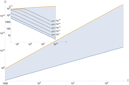
Figure 1: Query counts for negative log-norm systems. We consider homogeneous ODE systems $\dot{\boldsymbol{x}}=A\boldsymbol{x}$ for which $A$ has a negative log-norm $\mu=\lambda_{\textrm{max}}(A/2+A^{\dagger}/2)<0$, $\|A\|=1$ and set $\epsilon=10^{-10}$. (Main figure): For all such systems, the number of times $Q$ we need to query the block-encoding of $A$ to output the history lies in the shaded region shown, along a curve that depends on $\mu\in[-1,0]$. The scaling is sublinear unless $\mu=0$ (upper curve). For all these systems, the best prior bounds simply used that $C_{\textrm{max}}=1$ (which holds for every $\mu\leq 0$) and hence would return the upper (linear) curve. Hence the blue region corresponds to the query count improvement over prior methods such as [24]. (Inset): Same figure for the cost per unit time $Q/T$, and overlaid curves for different values $\mu$. Note that while one can obtain $Q/T=O(1)$, the increase of $Q/T$ in the above plot is due to us using a QLSA with complexity $\kappa_{L}\log\kappa_{L}$ [3]. This is done so as to provide the smallest query counts for regimes of interest.

I.3 Access model

$A$ and $\boldsymbol{b}$ in Eq. (1) are given. We discretize time in steps of size $h\leq 1/\|A\|$. Setting $\bar{t}=t/h$, $\bar{T}=T/h$, $\bar{A}=Ah$, $\bar{\boldsymbol{b}}=\boldsymbol{b}h$, we rescale the problem such that $\|\bar{A}\|\leq 1$ and the discrete times are $\bar{t}_{m}\in\{0,\dots,M=\bar{T}\}$ (and we increase $T$ slightly if needed to ensure integer separations). We shall assume this rescaling has been done and drop the bar for simplicity.

ODE parameter	Description
$A$, $\boldsymbol{b}$, $\boldsymbol{x}^{0}$	$A$ is the generator of the dynamics, $\boldsymbol{b}$ a forcing term, $\boldsymbol{x}^{0}$ the initial condition.
$T$	Target simulation time, normalized in units of the time-step $h$, which is chosen to be any value $h\leq 1/\|A\|$.
$\epsilon$	Target precision. Output is a quantum state $\epsilon$-close in $1$-norm to the final (2) or history (3) state.
$\omega$	Rescaling factor of the block-encoding of the generator $A$, Eq. (9).
$\kappa_{P}$, $\mu_{P}$	Stability / Lyapunov parameters: the generator $A$ satisfies $\|e^{At}\|\leq\sqrt{\kappa_{P}}e^{\mu_{P}(A)t}$ for $t\in[0,T]$.
$\lambda(T)$	Largest value between $T$ and the maximum forcing term to solution ratio:
	$\lambda(T)=\max\left\{\max_{t\in[0,T]}\frac{\|\boldsymbol{b}\|}{\|\boldsymbol{x}(t)\|},T\right\}.$
$\bar{g}(T)$	Ratio between the root mean square of the solution between $[0,T]$ and the solution at the final time:
	$\bar{g}(T)^{2}=\frac{1}{T+1}\sum_{m=0}^{T}\frac{\|\boldsymbol{x}(m)\|^{2}}{\|\boldsymbol{x}(T)\|^{2}}.$

Table 1: Summary of the algorithmic parameters and their description. Note that Hamiltonian simulation is the special case $A=-iH$, $\boldsymbol{b}=0$, $\kappa_{P}=1$, $\mu_{P}=0$, $\lambda(T)=T$, $\bar{g}(T)=1$.

Result	Final state	History state	Assumptions
Ref. [19]	$\tilde{O}(\kappa_{V}g(T){\color[rgb]{1,0,0}T}\log[\lambda(T)/\epsilon]\log(1/\epsilon))$	$\tilde{O}(\kappa_{V}{\color[rgb]{1,0,0}T}\log[\lambda(T)/\epsilon]\log(1/\epsilon))$	$\alpha(A)\leq 0$, $A$ diagonalizable via $V$
Ref. [24]	$\tilde{O}(C_{\textrm{max}}g(T){\color[rgb]{1,0,0}T}\log^{3/2}[\lambda(T)/\epsilon]\log(1/\epsilon))$	$\tilde{O}(C_{\textrm{max}}{\color[rgb]{1,0,0}T}\log^{3/2}[\lambda(T)/\epsilon]\log(1/\epsilon))$	$\|e^{At}\|\leq C_{\textrm{max}}$ for all $t\in[0,T]$
This work:	$\tilde{O}(C_{\textrm{max}}\bar{g}(T){\color[rgb]{1,0,0}T}\log[\lambda(T)/\epsilon]\log(1/\epsilon))$	$\tilde{O}(C_{\textrm{max}}{\color[rgb]{1,0,0}T}\log[\lambda(T)/\epsilon]\log(1/\epsilon))$	$\|e^{At}\|\leq C_{\textrm{max}}$ for all $t\in[0,T]$
This work:	$\tilde{O}(\kappa_{P}\bar{g}(T){\color[rgb]{1,0,0}T^{3/4}}\log[\lambda(T)/\epsilon]\log(1/\epsilon))$	$\tilde{O}(\kappa_{P}{\color[rgb]{1,0,0}\sqrt{T}}\log[\lambda(T)/\epsilon]\log(1/\epsilon))$	$A$ stable
This work:	$\tilde{O}(\bar{g}(T){\color[rgb]{1,0,0}T^{3/4}}\log[\lambda(T)/\epsilon]\log(1/\epsilon))$	$\tilde{O}({\color[rgb]{1,0,0}\sqrt{T}}\log[\lambda(T)/\epsilon]\log(1/\epsilon))$	$A$ with negative log-norm

Table 2: Asymptotic query complexity improvements for stable dynamics ($\alpha(A)<0$), where $\alpha(A):=\max_{i}\textrm{Re}\,\lambda_{i}(A)$, with $\lambda_{i}(A)$ being the eigenvalues of $A$. Third line: compared to the second line, we improve $g(T)=\max_{t\in[0,T]}\|\boldsymbol{x}(t)\|/\|\boldsymbol{x}(T)\|$ to $\bar{g}$ and remove the need for nested matrix inversion, which improves $\log^{3/2}[\lambda(T)/\epsilon]$ to $\log[\lambda(T)/\epsilon]$. Fourth line: as above, plus improves $T$ to $T^{3/4}$ (final state) or $T^{1/2}$ (history state). Fifth line: negative log-norm (special case of a stable matrix), improved over the previous treatment in Ref. [24], which uses the second line with $C_{\textrm{max}}=1$. The results of Ref. [19] are also recovered, with $g\rightarrow\bar{g}$.

Assume access to:

• A block-encoding of $A$, meaning a unitary $U_{A}$ with

  $$U_{A}\ket{\psi}\ket{0^{a}}=\frac{A}{\omega}\ket{\psi}\ket{0^{a}}+\ket{\perp},$$ (9)

  where $\ket{0^{a}}:=\ket{0}^{\otimes a}$, $\ket{\psi}$ is an arbitrary vector, $\omega$ is a rescaling factor required to encode $A$ into a unitary (we assume $\omega\geq 1$), and $\bra{0^{a}}\otimes I\ket{\perp}=0$. The values $(\omega,a)$ determine the quality of the block-encoding and depend on the specific form of $A$. For constructions for sparse and certain dense matrices achieving $\omega=O(1)$, see Refs [32, 33, 34, 35, 36].

• A unitary $U_{0}$ such that $U_{0}\ket{0}=\ket{x^{0}}$, encoding the initial condition $\boldsymbol{x}^{0}$ as a quantum state when applied to a reference state $\ket{0}$.

• (If $\boldsymbol{b}\neq\boldsymbol{0}$): A unitary $U_{b}$ such that $U_{b}\ket{0}=\ket{b}$, encoding $\boldsymbol{b}$ up to normalization.

The goal is to output a quantum state $\epsilon$-close in $1$-norm to Eq. (2), in the case of the final state, or Eq. (3), for the history state over the time interval $[0,T]$. The cost of obtaining $\ket{x_{F}}$ or $\ket{x_{H}}$ is evaluated via the query count, $\mathcal{Q}$, which is the number of times we need to apply the above unitaries. $\mathcal{Q}$ depends on the ODE parameters summarized in Table 2.

I.4 Summary of the algorithm

The solution of Eq. (1) can be formally written as

$$\boldsymbol{x}(t)=e^{At}\boldsymbol{x}^{0}+\int_{0}^{T}dt^{\prime}e^{At^{\prime}}\boldsymbol{b}.$$ (10)

By discretizing time, we can recursively approximate the solution at time $m$ from that at time $m-1$ via a Taylor series truncated at degree $k$:

$$\boldsymbol{x}(m)\approx\boldsymbol{x}^{m}:=T_{k}(A)\boldsymbol{x}^{m-1}+S_{k}(A)\boldsymbol{b},$$ (11)

where $T_{k}(x)=\sum_{j=0}^{k}x^{j}/j!$ and $S_{k}(x)=\sum_{j=1}^{k}x^{j-1}/j!$. One can upper bound the required $k$ such that the time-discretization relative error is at most $\epsilon_{\mbox{\tiny TD}}$, meaning

$$\|\boldsymbol{x}^{m}-\boldsymbol{x}(mh)\|\leq\epsilon_{\mbox{\tiny TD}}\|\boldsymbol{x}(mh)\|,\quad m=0,\dots,T.$$ (12)

Exploiting Theorem 3 in Ref. [24], we find a value for the truncation degree, $k$, that suffices, see Appendix A.2. In particular, $k=O\left(\log\frac{\lambda(T)}{\epsilon_{\mbox{\tiny TD}}}\right)$.

The recursive equations are embedded, as in Ref. [19], into a linear system $L$ whose blocks only contain matrices proportional to $A$ or the identity. This linear system takes the form $L\boldsymbol{y}=\boldsymbol{c}$, where $\boldsymbol{y}$ encodes the dynamical solution at all times $[0,T]$. In fact, an idling parameter $p$ in the linear system allows us to embed the trivial evolution generated by $A=0$ for $p$ time-steps at the end, which increases the amplitude of the final state component. This is useful if we are trying to output $\ket{x_{F}}$.

This linear system of equations is solved via QLSA, see the schematics in Fig. 2. The unitaries O1, O2, O3 are used to construct a block-encoding of the linear system matrix $L$ and the vector of constants $\boldsymbol{c}$. The number of times these need to be called in the QLSA algorithm is classically precomputed as we shall see in Theorem 2. The output solution is post-processed via amplitude amplification as needed, to get either a quantum state encoding an approximation of the final state (2) or of the history state (3).

To compute the (non-asymptotic) query count upper bounds of the ODE algorithm we need to construct the linear system block-encoding, determine the QLSA parameters, analyze the output processing success probability and how exactly the various error sources (time-discretization, finite precision of the QLSA) compound. Here we report the main results.

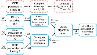
Figure 2: Algorithm schematics. ODE algorithm schematics. (Red, dashed): classical precomputations. (Blue, solid): quantum operations. The algorithm reduces solving the ODE to solving a linear system of equations. O1, O2, O3 are the three oracles given on the previous page.

I.5 Asymptotic complexity and fast-forwarding.

The asymptotic complexity obtained through our new analysis improves over state-of-the-art as shown in Table 2. Note that Berry et al. [19] assume that $A$ has $\alpha(A)\leq 0$ and is diagonalizable via a matrix $V$ whose condition number $\kappa_{V}$ is known. This is recovered as a special case in our framework by taking $(\kappa_{P},\mu_{P})=(\kappa_{V}^{2},0)$. Instead, if we drop the diagonalizability assumption and we only have a uniform bound as in Eq. (8), we can take $(\kappa_{P},\mu_{P})=(C_{\textrm{max}}^{2},0)$. This recovers the results in [24] with slightly improved asymptotics and within the simpler encoding of Berry et al. [19], whose linear system construction does not require matrix inversion [24] or exponentiation [23].

However for stable systems, $\alpha(A)<0$, we obtain significant improvements from our strengthened condition number bounds. One might expect that simulating ODE systems could in general be harder than the Schrödinger equation, since one incurs various overheads in transforming the problem into a form suitable for a quantum computer. Here we sharpen this relation by showing that quantum dynamics are at the boundary of stable dynamics, and that for the latter the condition number of the linear system associated to the ODE scales sublinearly in the target simulation time $T$:

Theorem 1 (Fast-forwarding of stable systems).

Let $A$ be a stable matrix and let $P>0$ be any matrix that satisfies the Lyapunov inequality $PA+A^{\dagger}P<0$. Then outputting the final state requires

$$\tilde{O}(\sqrt{\kappa_{P}}\bar{g}(T)T^{3/4}\log[\lambda(T)/\epsilon]),$$ (13)

queries to the oracles for $A$, $\boldsymbol{b}$ and $\boldsymbol{x}^{0}$, while outputting the history state requires

$$\tilde{O}(\sqrt{\kappa_{P}}T^{1/2}\log[\lambda(T)/\epsilon]),$$ (14)

queries to these oracles.

See Appendix G for the full technical statement and proof. This gives sublinear scaling in $T$ when $\log(\lambda(T))\bar{g}(T)=o(T^{1/4})$ for outputting the final state or when $\log\lambda(T)=o(T^{1/2})$, for outputting the history state. It also gives improvements beyond this regime. If $\log\lambda(T)=O(T)$, which occurs for an exponentially decaying solution, the time scaling for the history state output according to our analysis is $O(T^{3/2})$, whereas the best scaling using prior analysis is $O(T^{2})$ or $O(T^{5/2})$, see Table 2. Speedups under the similar norm caveats were known for special classes of dynamics ($A$ for which we access a unitary that diagonalizes it; $A=-H^{2}$ for some Hermitian $H$, as in [37]). Our result paves the way to much cheaper ODE simulations than previously thought.

I.6 Detailed query counts of the ODE-solver.

So far we have discussed asymptotics, but in fact we can compute analytic query complexity upper bounds. Since the final expression is cumbersome, we describe it via a sequence of straightforward replacements.

Theorem 2 (Explicit query counts for ODE-solver).

Given a linear ODE of the form $\dot{\boldsymbol{x}}=A\boldsymbol{x}+\boldsymbol{b}$, $\boldsymbol{x}(0)=\boldsymbol{x}^{0}$, assume access to $U_{A}$, $U_{0}$ in (O1), (O2), as well as $U_{\boldsymbol{b}}$ in (O3) if $\boldsymbol{b}\neq\boldsymbol{0}$. The final (2) and history (3) states can be prepared with a number of queries $\mathcal{Q}$ to $U_{A}$, $2\mathcal{Q}$ queries to $U_{0}$ and, if $\boldsymbol{b}\neq\boldsymbol{0}$, $2\mathcal{Q}$ queries to $U_{b}$. $\mathcal{Q}$ can be analytically upper bounded as shown in the diagram below:

1. Set the time discretization error $\epsilon_{\mbox{\tiny TD}}=\epsilon/8$.

2. Compute the Taylor truncation:

   $$k=\left\lceil\frac{3\log(x_{*})/2+1}{\log[1+\log(x_{*})/2]}-1\right\rceil,$$ (15)

   with $x^{*}\geq\max\{\frac{Te^{3}}{\epsilon_{\mbox{\tiny TD}}}(1+Te^{2}\max_{t\in[0,T]}\frac{\|\boldsymbol{b}\|}{\|\boldsymbol{x}(t)\|}),10\}$.

3. For the history state, we set an idling parameter $p$ to $p=0$. For the final state, we set $p=\lceil T^{1/2}/(k+1)\rceil(k+1)$ in the case that $A$ is stable, and $p=\lceil T/(k+1)\rceil(k+1)$ otherwise.

4. Compute $\omega_{\tilde{L}}=\frac{1+\sqrt{k+1}+\omega}{\sqrt{k+1}+2}$.

5. Compute the upper bound on the condition number

   $$\kappa_{L}\leq \left[(1+\epsilon_{\mbox{\tiny TD}})^{2}\left(1+g(k)\right)\kappa_{P}\left(p\frac{1-e^{2T\mu_{P}(A)+2\mu_{P}(A)}}{1-e^{2\mu_{P}(A)}}\right.\right.$$

   $$\left.\left.+I_{0}(2)\frac{e^{2\mu_{P}(A)(T+2)}+T+1-e^{2\mu_{P}(A)}(2+T)}{(1-e^{2\mu_{P}(A)})^{2}}\right)\right.$$

   $$\left.+\frac{p(p+1)}{2}+(p+Tk)(I_{0}(2)-1)\right]^{1/2}\times(\sqrt{k+1}+2),$$ (16)

   where $g(k)=\sum_{s=1}^{k}\left(s!\sum_{j=s}^{k}1/j!\right)^{2}\leq ek$ and $I_{0}(2)\approx 2.2796$.

6. Fix $K=(3-e)^{2}$ for the inhomogeneous case ($\boldsymbol{b}\neq\boldsymbol{0})$ and $K=1$ for the homogeneous case $(\boldsymbol{b}=\boldsymbol{0})$. For outputting the history state compute the success probability

   $$\textrm{Pr}_{H}\geq\frac{K}{K-1+I_{0}(2)}\geq\begin{cases}0.058\quad\boldsymbol{b}\neq\boldsymbol{0}\\ 0.438\quad\boldsymbol{b}=\boldsymbol{0},\end{cases}$$ (17)

   and for outputting the final state compute

   $$\textrm{Pr}_{F}\geq\frac{1}{(1-\frac{I_{0}(2)-1}{(p+1)K})+(T+1)\frac{I_{0}(2)-1}{(p+1)K}\left(\frac{1+\epsilon_{\mbox{\tiny TD}}}{1-\epsilon_{\mbox{\tiny TD}}}\right)^{2}\bar{g}^{2}}.$$ (18)

7. Compute $\epsilon_{\mbox{\tiny LS}}=\epsilon\frac{\textrm{Pr}_{H,F}}{4+\epsilon}$.

8. Compute $\mathcal{Q}_{QLSA}=\mathcal{Q}_{QLSA}(\omega_{\tilde{L}},\kappa_{L},\epsilon_{\mbox{\tiny LS}})$, the best available query counts for QLSA given the parameters $\omega_{\tilde{L}},\kappa_{L},\epsilon_{\mbox{\tiny LS}}$. Here we use the closed formula for $\mathcal{Q}_{QLSA}(\omega,\kappa,\epsilon)$ from Ref. [3], also provided in Appendix H.

9. Compute $\mathcal{A}(\textrm{Pr}_{H,F})$, the query counts for amplitude amplification from success probability $\textrm{Pr}_{H,F}$ (see, e.g., Ref. [38]), or $\mathcal{A}(\textrm{Pr}_{H,F})=1/\textrm{Pr}_{H,F}$ if we sample till success.

10. Finally, $\mathcal{Q}=\mathcal{Q}_{QLSA}\times\mathcal{A}$.

The total logical qubit count for the algorithm is $a+12+\lceil\log_{2}[((T+1)(k+1)+p)N]\rceil$.

This gives the first detailed counts for solving ODEs on a quantum computer, a crucial step to determining what problems of interest could be run on early generations of fault-tolerant quantum computers. These results also provide explicit targets for future work to improve on.

I.7 Query counts for history state of homogeneous ODEs.

To illustrate the result, we apply Theorem 2 to evaluate the non-asymptotic cost of outputting the history state for a homogeneous system of ODEs with negative (Euclidean) log-norm. Hence, $\lambda(T)=T$, $\kappa_{P}=1$, $\mu_{P}(A)=\mu(A)$. We shall set $\epsilon=10^{-10}$ and $\omega=1$ ( here $\omega$ denotes the block-encoding scale factor. The total cost will be increased by about a factor of $\omega$ if $\omega>1$). $T$ is measured in units of $h$, where $h\leq 1/\|A\|$. In Fig. 1 we plot $\mathcal{Q}$ as a function of $T$ for all possible $\mu(A)$, and we recall that $\mu(A)\in[-1,0]$, with $\mu(A)\rightarrow 0^{-}$ corresponding to the $\alpha(A)\geq 0$ case with $C_{\textrm{max}}=1$. We computed $\mathcal{Q}$ under the assumption that we do not perform amplitude amplification, but simply repeat till success, which is potentially more convenient since the success probability is high. We obtain the shaded region in Fig. 1, which interpolates from the linear in $T$ scaling to the best possible $\sqrt{T}$ scaling. The upper curve in Fig. 1 can be upper bounded for $T\in[10^{6},10^{15}]$ and $\epsilon=10^{-10}$ as $Q\leq 10300T\log T$. For the lower curve, $Q\leq 11900\sqrt{T}\log T$ with the same specifications. We see that incorporating knowledge about stability can lead to orders of magnitude improvements in the query counts. An additional factor of $3$ saving can also potentially be achieved from generalized quantum signal processing [39], which removes the need for LCU in the QLSA of Ref. [3].

I.8 Fast-forwarding of nonlinear differential equations.

We discuss an application to nonlinear differential equations. Ref. [24] starts with a set of nonlinear (quadratic) ODEs with $R<1$ (where $R$ can be viewed as a form of Reynold’s number) and a linear term with negative log-norm, and maps it into a system of linear ODEs via the Carleman embedding method. The resulting ODE has a generator $A$ with negative log-norm, and using the prior state-of-the-art (second line of Table 2 with $C_{\textrm{max}}=1$) a scaling at least linear in $T$ was obtained (Theorem 8 of Ref. [24] for the final state problem). Instead, we can use the improved scalings in the fifth line of Table 2, which could potentially give a sublinear scaling in $T$ for encoding the solution of the nonlinear system of ODEs in a quantum state. This will be explored in more detail in future work.

II The algorithm

The algorithm is based on the novel analysis of Ref. [19].

(1) Linear system encoding: We introduce $3$ registers $\ket{m,j,n}$, and proceed similarly to Ref. [19]. Register $m$ is a clock degree of freedom, labeling the solution at each time-step within $[0,T]$, plus potentially further idling steps to increase the amplitude of the solution at the final state, if necessary. It takes values $m=0,\dots,T+p/(k+1)$, where $p$ is a multiple of $k+1$ to be fixed. The $j$ register is used to compute Taylor sums, $j=0,\dots,k$. Finally, $n$ labels the components of the vector $\boldsymbol{x}$, $n=1,\dots,N$. We encode data about the solution to the ODE problem into the solution $\boldsymbol{y}:=L^{-1}\boldsymbol{c}$ of a linear system (Appendix B):

$$L\boldsymbol{y}=\boldsymbol{c},$$ (19)

where $L=L_{1}+L_{2}+L_{3}$, and

$$L_{1}:= I\otimes I\otimes I,$$ (20)

$$L_{2}:= -\sum_{m=0}^{T-1}\sum_{j=1}^{k}\ket{m,j}\!\!\bra{m,j-1}\otimes\frac{A}{j}$$

$$-\theta(p)\sum_{m=T}^{T+\frac{p}{k+1}-1}\sum_{j=1}^{k}\ket{m,j}\!\!\bra{m,j-1}\otimes I,$$ (21)

$$L_{3}:= -\sum_{m=0}^{T-1}\sum_{j=0}^{k}\ket{m+1,0}\!\!\bra{m,j}\otimes I,$$ (22)

with the Heaviside function $\theta(p)=0$ for $p=0$ and $\theta(p)=1$ for $p>0$. The term $L_{2}$ generates Taylor components, which are summed at each $m$ by $L_{3}$ to generate a truncated Taylor series that approximates the dynamics up to $m=T$. If $p\geq k+1$, from $m=T$ to $m=T+p/(k+1)-1$ and for all $j=0,\dots,k$, so $p$ steps overall, the term $L_{2}$ generates ‘idling’, which allows for an increase of the amplitude of the final state component. In Eq. (19) we set

$$\boldsymbol{c}=[\overbrace{\boldsymbol{x}^{0},\underbrace{\boldsymbol{b},\boldsymbol{0},\dots,\boldsymbol{0}}_{k}}^{m=0},\dots,\overbrace{\boldsymbol{0},\underbrace{\boldsymbol{b},\boldsymbol{0},\dots,\boldsymbol{0}}_{k}}^{m=M-1},\underbrace{\boldsymbol{0},\dots,\boldsymbol{0}}_{1+p}].$$ (23)

It can be shown that the solution to this system can be split up as $\boldsymbol{y}=\boldsymbol{x}_{H}^{\epsilon_{\mbox{\tiny TD}}}+\boldsymbol{x}_{\textrm{junk}}$, where

$$\boldsymbol{x}_{H}^{\epsilon_{\mbox{\tiny TD}}}=(\boldsymbol{x}^{0},\boldsymbol{0},\dots,\boldsymbol{0},\boldsymbol{x}^{1},\boldsymbol{0},\dots,\boldsymbol{0},\underbrace{\boldsymbol{x}^{T},\dots,\boldsymbol{x}^{T}}_{1+p})$$ (24)

and $\boldsymbol{x}_{\textrm{junk}}$ is an orthogonal ‘junk’ component, that is unwanted, and can be removed by post-selection. When we output the history state, we set $p=0$ and $\boldsymbol{x}_{H}^{\epsilon_{\mbox{\tiny TD}}}$ (as a normalized quantum state $\ket{x^{\epsilon_{\mbox{\tiny TD}}}_{H}}$) provides a discrete approximation to the exact history state encoded in Eq. (3) (Appendix A.2):

$$\|\ket{x^{\epsilon_{\mbox{\tiny TD}}}_{H}}-\ket{x_{H}}\|\leq 2\epsilon_{\mbox{\tiny TD}}\;.$$ (25)

Instead, when we output the final state, we set $p>0$ and target the components $\boldsymbol{x}^{T}$ with amplitude amplification.

(2) Solving the linear system: Eq. (19) is tackled using the best available asymptotic [2] and non-asymptotic [3] query complexity upper bound for QLSA. The running cost depends on three parameters:

1. The cost of constructing a block-encoding of $L$ from that of $A$.

2. An upper bound on the condition number of $L$, i.e., on $\kappa_{L}:=\|L\|\|L^{-1}\|$.

3. The QLSA does not output the ideal solution $\ket{y}$, but a quantum state $\rho$ which is $\epsilon_{\mbox{\tiny LS}}$-close to it in $1-$norm. The cost depends on $\epsilon_{\mbox{\tiny LS}}$.

All three will be determined from the ODE parameters.

(a) Constructing the linear system block-encoding. We prove that $\|L\|\leq\omega_{k}:=\sqrt{k+1}+2$. Hence we define $\tilde{L}=L/\omega_{k}$, $\tilde{\boldsymbol{c}}=\boldsymbol{c}/\omega_{k}$ and solve the problem $\tilde{L}\boldsymbol{y}=\tilde{\boldsymbol{c}}$. This has $\|\tilde{L}\|\leq 1$, as normally required by QLSA.

The detailed running cost of a QLSA is in terms of calls to a unitary block-encoding $U_{\tilde{L}}$ of $\tilde{L}$ and a state preparation unitary $U_{\tilde{c}}$ of $\tilde{\boldsymbol{c}}$. These need to be constructed from the available unitaries $U_{A}$, $U_{b}$, $U_{0}$ (details in Appendix C). Concerning $U_{\tilde{c}}$, it can be constructed with a single call to both $U_{0}$ and $U_{b}$. As for $U_{\tilde{L}}$, we construct an $(\omega_{\tilde{L}},a+6,0)$-block-encoding of $\tilde{L}$ with a single call to $U_{A}$, where $\omega_{\tilde{L}}=(1+\sqrt{k+1}+\omega)/\omega_{k}$, as given in Theorem 2. The QLSA requires $6$ further ancilla qubits, as well as $\lceil\log_{2}[((T+1)(k+1)+p)N]\rceil$ qubits to encode $\tilde{L}$.

(b) Condition number bound. Recall that the Lyapunov analysis leads to stability parameters $(\kappa_{P},\mu_{P}(A))$. In Appendix D we find the upper bound on $\kappa_{L}$ in terms of the stability properties as given in Theorem 2, inequality (16).

We set $p=0$ for the case where we output the history state. For the case where we output the final state, we take $p=\lceil T^{1/2}/(k+1)\rceil(k+1)$ in the case that $A$ is stable, and $p=\lceil T/(k+1)\rceil(k+1)$ otherwise. For both final and history state, we then have $\kappa_{L}=O(T^{1/2}k)$ in the stable case and $\kappa_{L}=O(Tk)$ otherwise. The better scaling of this bound leads to the improvements in Table 2.

Also note that in Appendices B and D we provide a broader analysis of idling, where we allow varying amplifications at each discrete time-step, specified by integers $\{p_{m}:m=0,1,\dots,T\}$. This allows us to increase the amplitude of selected terms $\ket{x(t_{m})}$ in the history state (3), which can be understood as applying a filter to the dynamical data.

(c) Required precision. To determine $\epsilon_{\mbox{\tiny LS}}$, we first need to analyze the output processing.

(3) Output processing: We first present an analysis assuming we access the idealized linear system solution $\ket{y}$, and then consider the effect of finite precision.

Idealized analysis. The ideal solution of the linear system encodes ODE data in the sense that we recover a state close to $\ket{x_{H,F}}$ by performing a projective measurement $\{\Pi_{H,F},I-\Pi_{H,F}\}$ on the auxiliary/clock registers. Specifically, if

$$\Pi_{H}=I\otimes\ket{0}\!\!\bra{0}\otimes I,\quad\Pi_{F}=\sum_{m=T}^{T+p/(k+1)}\ket{m}\!\!\bra{m}\otimes I\otimes I,$$

we have

$$\Pi_{H}\ket{y}\!\!\bra{y}\Pi_{H}=\textrm{Pr}_{H}\ket{x^{\epsilon_{\mbox{\tiny TD}}}_{H}}\!\!\bra{x_{H}^{\epsilon_{\mbox{\tiny TD}}}},$$ (26)

where $\|\ket{x^{\epsilon_{\mbox{\tiny TD}}}_{H}}-\ket{x_{H}}\|\leq 2\epsilon_{\mbox{\tiny TD}}$ from Eq. (3) and

$$\textrm{Tr}_{CA}[\Pi_{F}\ket{y}\!\!\bra{y}\Pi_{F}]=\textrm{Pr}_{F}\ket{x^{T}}\!\!\bra{x^{T}},$$ (27)

where the trace discards clock and ancilla qubits and $\|\ket{x^{T}}-\ket{x_{F}}\|\leq 2\epsilon_{\mbox{\tiny TD}}$ (Appendix A.2).

The values $\textrm{Pr}_{H,F}$ are success probabilities of the corresponding measurements. For outputting the history state we obtain the success probability in (17), so the overhead to repeat the measurement until success or via amplitude amplification is $O(1)$. For output of the final state we have the expressions given in Theorem 2, which imply

$$\textrm{Pr}_{F}\geq\begin{cases}O(\bar{g}^{-2}T^{-1/2})\quad\textrm{for $A$ stable,}\\ O(\bar{g}^{-2})\quad\textrm{otherwise}.\end{cases}$$ (28)

Using amplitude amplification we have an overhead of $O(1/\sqrt{\textrm{Pr}_{F}})$ repetitions.

Error analysis. We now consider the effect of the finite precision $\epsilon_{\mbox{\tiny LS}}$ of the QLSA and go back to point (c) of the previous section, i.e. answer the question of what linear solver error $\epsilon_{\mbox{\tiny LS}}$ suffices, as well as what discretization error $\epsilon_{\mbox{\tiny TD}}$ we need to target, given a total error budget $\epsilon$.

In Appendix F, we find that the protocol presented (including the output processing) returns a quantum state $\tilde{\sigma}_{H,F}$ satisfying

$$\|\sigma_{H,F}-\ket{x_{H,F}}\!\!\bra{x_{H,F}}\|_{1}\leq\frac{2\epsilon_{\mbox{\tiny LS}}}{\textrm{Pr}_{H,F}-\epsilon_{\mbox{\tiny LS}}}+4\epsilon_{\mbox{\tiny TD}},$$ (29)

with a success probability at least $\textrm{Pr}_{H,F}-\epsilon_{\mbox{\tiny LS}}$. If we choose the two terms in (29) to have equal magnitude, then it suffices to take errors as given in Theorem 2.

III Outlook

Quantum computers are expected to be a disruptive technology for the simulation of quantum mechanical problems. We presently do not know if quantum computing will have a similar impact on important classes of classical dynamical problems. What we do know, however, is that there is no scarcity of computational problems of broad relevance, such as in fluid dynamics and plasma physics, which are often under-resolved on today’s largest computers and will remain so in the foreseeable future. If we could identify such use cases and provide a fully compiled quantum algorithm with reasonable resource estimates, then the scientific and technological value of quantum computers would be substantially increased. If this development follows a similar line to that for quantum chemistry, increasingly better algorithms and resource estimates will be required, likely starting from very high resource counts and then pushing numbers down for specific problem instances. We see the present work as a step in this direction. In giving the first detailed query count analysis for the general problem of solving linear differential equations on a quantum computer, we hope to set a signpost for improved resource estimates in the future, and also set the stage for a detailed analysis of the cost of solving nonlinear differential equations. The fast-forwarding results, furthermore, suggest these algorithms may be significantly less costly than previously thought in certain regimes.

Authors contributions: ML conceived the core algorithm analysis and derived an early version of the results. ML and DJ derived the new condition number upper bound, obtained the fast-forwarding results via the stability analysis, computed the detailed cost upper bound for the ODE solver, derived the success probabilities lower bounds and the error propagation analysis. RBL and ATS contributed to the stability and discretization methods. ML and DJ wrote the paper and RBL, SP, ATS contributed to structuring and reviewing the article. SP and ATS coordinated the collaboration.

Acknowledgements: RBL and ATS are supported by the U.S. Department of Energy through the Los Alamos National Laboratory, under the ASC Beyond Moore’s Law project. Los Alamos National Laboratory is operated by Triad National Security, LLC, for the National Nuclear Security Administration of U.S. Department of Energy (Contract No. 89233218CNA000001). Many thanks to Yiğit Subaşı for useful discussions on these topics and Michał Stęchły and Mark Steudtner for useful comments on a draft of this work.

Appendices

Appendix A Analysis of the dynamics

A.1 Stability and Lyapunov relations

For this discussion we refer to Ref. [30, 40] for further details, but many more sources can be found on the topic.

In general, we do not want the dynamics $\boldsymbol{x}(t)$ to blow-up in terms of norm as $t\rightarrow\infty$. A necessary condition for this to happen for every initial condition is that the matrix $A$ does not have any eigenvalues $\lambda_{i}(A)$ with positive real parts. This motivates the definition $\alpha(A):=\max_{i}\{Re(\lambda_{i}(A))\}$, and if $\alpha(A)<0$, then $A$ is said to be stable. We have that

$$\lim_{t\rightarrow\infty}\|e^{At}\|=0,$$ (30)

if and only if $A$ is stable. A necessary and sufficient condition for stability is that there is a matrix $P>0$ (strictly positive) such that

$$PA+A^{\dagger}P=-Q,$$ (31)

for some $Q>0$. This is known as the Lyapunov equation. This condition is related to the existence of quadratic Lyapunov functions for the dynamics generated by $A$. Indeed, it can be shown that for the homogeneous linear system $\frac{d\boldsymbol{x}(t)}{dt}=A\boldsymbol{x}(t)$, Eq. (31) holds if and only if the quadratic form $V(\boldsymbol{x}):=\boldsymbol{x}^{\dagger}P\boldsymbol{x}$ obeys

$$\frac{d}{dt}V(\boldsymbol{x}(t))=-\boldsymbol{x}^{\dagger}(t)Q\boldsymbol{x}(t)<0,$$ (32)

along all trajectories $\boldsymbol{x}(t)$. The non-negative quadratic form $V(\boldsymbol{x})$ can be viewed as a form of energy function, and from the fact that $\dot{V}(\boldsymbol{x})=-\boldsymbol{x}^{\dagger}(t)Q\boldsymbol{x}(t)\leq-cV(\boldsymbol{x})$, for some constant $c>0$ it follows from Grönwall’s inequality that there is another constant $C$ such that

$$\|\boldsymbol{x}(t)\|\leq Ce^{-ct/2}\|\boldsymbol{x}(0)\|,$$ (33)

for all $t\geq 0$. This is called global exponential stability for the dynamics. Note that the above discussion still holds in the $\alpha(A)=0$ case, but the strict inequality $c>0$ is replaced with the non-strict one $c\geq 0$, allowing $c=0$ and $C$ not constant.

Global exponential stability relates to the trajectories of the dynamics, but for the analysis of our algorithm, we instead require conditions on the exponentiated matrix $A$. While, asymptotically, homogeneous stable systems decay, they can still display transient increases in the norm $\|e^{At}\|$ for finite times. We can provide sharper measures of the early-time regime via the logarithmic norm (or log-norm for short) of $A$, denoted $\mu(A)$ and defined as the initial growth rate

$$\mu(A):=\frac{d}{dt^{+}}\|e^{At}\|_{t=0}=\lim_{h\rightarrow 0^{+}}\frac{1}{h}(\|I+Ah\|-1).$$ (34)

The definition depends on the particular choice of norm used, and unless otherwise stated we shall assume the operator norm is used. A significant property of the log-norm is that it is the smallest $\beta\in\mathbb{R}$ such that $\|e^{At}\|\leq e^{\beta t}$ for all $t\geq 0$. In the case of the operator norm, its value can also be calculated from

$$\mu(A)=\frac{1}{2}\lambda_{\textrm{max}}(A+A^{\dagger})=\max_{\|\boldsymbol{x}\|\neq 0}\textrm{Re}\,\frac{\langle A\boldsymbol{x},\boldsymbol{x}\rangle}{\langle\boldsymbol{x},\boldsymbol{x}\rangle},$$ (35)

where $\lambda_{\textrm{max}}(X)$ denotes the largest eigenvalue of any Hermitian matrix $X$. If $\mu(A)<0$ then the system is stable, but even if $\mu(A)>0$ stability can still occur. However, in this case the bound $\|e^{At}\|\leq e^{\mu(A)t}$ is no longer useful. To account for this regime one can introduce a different log-norm:

$$\mu_{P}(A)=\max_{\|\boldsymbol{x}\|\neq 0}\textrm{Re}\,\frac{\langle PA\boldsymbol{x},\boldsymbol{x}\rangle}{\langle P\boldsymbol{x},\boldsymbol{x}\rangle},$$ (36)

the log-norm with respect to the elliptical norm induced by $P$. This can be seen as an initial growth rate with respect to the norm induced by $P$ [Lemma 3.31, Ref. [30]]. Note that stability implies $\mu_{P}(A)<0$ for some $P>0$. In particular, denote the condition number of $P$ by $\kappa_{P}$. One then has [Theorem 3.35, Ref. [30]]

$$\|e^{At}\|\leq\sqrt{\kappa_{P}}e^{\mu_{P}(A)t},$$ (37)

which accounts for potential increases of $\|e^{At}\|$ in a transient regime.

Finally, we note that in the case of Schrödinger evolution under $A=-iH$ for some Hamiltonian $H$, we have a constant norm for the dynamics, and so the system is not stable in the above sense – in the literature this case is called “marginally stable". Quantum dynamics, or any other linear dynamics with $A$ having eigenvalues with vanishing real parts, are not stable under arbitrarily small perturbations in $A$, while stable systems do allow small perturbations while still remaining stable.

A.2 Time discretization error analysis

We now describe the formal solution to the ODE, and the discretized solution that our algorithm will return. The solution of Eq. (1) can be formally written as

$$\boldsymbol{x}(t)=e^{At}\boldsymbol{x}(0)+\int_{0}^{t}dt^{\prime}e^{At^{\prime}}\boldsymbol{b},$$ (38)

for any $t\in[0,T]$. We proceed by splitting the time interval up into $M$ equal-sized sub-intervals of width $h$, so that we can approximate the dynamics at each of these time points. The exact solution data at these points are $\boldsymbol{x}(0),\boldsymbol{x}(h),\dots,\boldsymbol{x}(mh),\dots,\boldsymbol{x}(Mh)=\boldsymbol{x}(T)$. We shall approximate $\boldsymbol{x}(mh)$ with $\boldsymbol{x}^{m}$, which is a vector obtained from a discrete sequence of evolutions obtained from a truncated Taylor series for the exponential $e^{At}$. In particular we use

$$T_{k}(Ah) :=\sum_{j=0}^{k}\frac{1}{j!}(Ah)^{j}$$

$$S_{k}(Ah) :=\sum_{j=1}^{k}\frac{1}{j!}(Ah)^{j-1},$$ (39)

to approximate the exponentials needed to order $k$. The discretized dynamics is now defined recursively by $\boldsymbol{x}^{0}:=\boldsymbol{x}(0)$, and

$$\boldsymbol{x}^{m}:=T_{k}(Ah)\boldsymbol{x}^{m-1}+S_{k}(Ah)\boldsymbol{b},$$ (40)

for all $m=1,\dots,M$. The following result gives the condition on the truncation order $k$ so as to obtain a target relative error $\epsilon_{\mbox{\tiny TD}}$.

Lemma 3 (Time-discretization error, Theorem 3 of Ref. [24]).

Let $r(T)$ be a constant such that $r(T)\geq\|\boldsymbol{b}\|/\|\boldsymbol{x}(t)\|$ for all $t\in[0,T]$. If we choose the integer $k$ such that

$$(k+1)!\geq\frac{Me^{3}}{\epsilon_{\mbox{\tiny TD}}}(1+Te^{2}r(T)),$$ (41)

then it follows that the relative time-discretization error obeys

$$\|\boldsymbol{x}(mh)-\boldsymbol{x}^{m}\|\leq\epsilon_{\mbox{\tiny TD}}\|\boldsymbol{x}(mh)\|,$$ (42)

for all $m=0,1,\dots M$.

We can provide a sufficient value of $k$ required from the following lemma.

Lemma 4 (Sufficient truncation scale).

The choice

$$k=\left\lceil\frac{3\log(x_{*})/2+1}{1+\log(\log(x_{*})/2e+1/e)}-1\right\rceil$$ (43)

with $x^{*}=\frac{Te^{3}}{h\epsilon_{\mbox{\tiny TD}}}(1+Te^{2}r(T))$ suffices to obtain a relative time-discretization error $\epsilon_{\mbox{\tiny TD}}$ over all $M=T/h$ time-steps of the dynamics. In particular $k=O(\log\left(\lambda(T)/\epsilon_{\mbox{\tiny TD}}\right))$.

Proof.

From Lemma 3 it suffices to take $(k+1)!\geq x_{*}$. From the Stirling approximation we have that

$$n!\geq\left(\frac{n}{e}\right)^{n},$$ (44)

so it suffices to take $(\frac{k+1}{e})^{k+1}\geq x^{*}$, i.e., $k=\lceil f^{-1}(x_{*})\rceil-1$ where we define $f(x)=\left(\frac{x}{e}\right)^{x}$. However we have that for any $x>0$

$$f^{-1}(x)=\exp\left[W\left(\frac{\log x}{e}\right)+1\right],$$ (45)

where $W(x)$ is the principal branch of the Lambert W-function. We now use the upper bound

$$e^{W(x)}\leq\frac{x+y}{1+\log y},$$ (46)

which holds for any $x>-1/e$ and any $y>1/e$ [41].

In our case this reads

$$e^{W(\log(x)/e)}\leq\frac{\log(x)/e+y}{1+\log y}$$ (47)

We now take $y=1/e+\log(x)/2e$, and therefore have that

$$f^{-1}(x)-1\leq e^{W(\log(x)/e)+1}-1\leq\frac{3\log(x)/2+1}{1+\log(\log(x)/2e+1/e)}-1=O(\log(x)).$$ (48)

We now set $x=x_{*}$ and round up to the nearest integer to obtain the result claimed. ∎

This expression shows that $k$ grows at worst logarithmically in time, $k=O(\log(T))$, for the homogeneous ODE case, while for the inhomogenous case one can generally obtain $k=O(T)$ if $\lambda(T)$ decreases exponentially in $T$, as we discuss later.

For homogeneous regimes of interest the value of $k$ is quite mild. For example, taking $\lambda(T)=0$, $M=10^{6}$ and $\epsilon_{\mbox{\tiny TD}}=10^{-9}$ the bound returns $k=19$ (rounding up $18.2$). Directly solving numerically the original bound in Lemma 3 for $k$ gives $k=18$, so the analytical bound is relatively tight.

The recursively defined dynamics generates terms such as $T_{k}(Ah)^{m}$, which approximate $(e^{Ah})^{m}=e^{Amh}$ for all $m=0,1,\dots,M$. For the condition number analysis we need an estimate on how well the truncated expression $T_{k}(Ah)^{m}$ approximates the exact exponential $e^{Amh}$ for the continuous dynamics. The next result determines the relative error for these matrices in the discrete dynamics.

Lemma 5 (Truncation error for dynamics, Lemma 13 of Ref. [24]).

Let $k$ obey the time-discretization condition given by Equation (41). Then for all $m=0,1,\dots M$ we have the following relative error for the norm $\|T_{k}(Ah)^{m}\|$ relative to $\|e^{Ahm}\|$.

$$\|T_{k}(Ah)^{m}\|\leq\|e^{Ahm}\|(1+\epsilon_{\mbox{\tiny TD}}),$$ (49)

Note that so far we discussed time-discretization errors at the level of unnormalized solution vectors, but these can be readily translated into errors on the normalized quantum states.

Lemma 6.

For any two vectors

$$\ket{z}=\frac{1}{\|\boldsymbol{z}\|}(\boldsymbol{z}^{1},\dots,\boldsymbol{z}^{J}),\quad\quad\ket{\tilde{z}}=\frac{1}{\|\tilde{\boldsymbol{z}}\|}(\tilde{\boldsymbol{z}}^{1},\dots,\tilde{\boldsymbol{z}}^{J}),$$ (50)

if the relative error of each component is upper bounded as $\|\boldsymbol{z}^{j}-\tilde{\boldsymbol{z}}^{j}\|\leq\delta\|\tilde{\boldsymbol{z}}_{j}\|$ for all $j=1,\dots,J$, then it follows that for the corresponding normalized vectors we have

$$\|\ket{z}-\ket{\tilde{z}}\|\leq 2\delta.$$ (51)

Proof.

$$\|\ket{z}-\ket{\tilde{z}}\| =\left\|\frac{\boldsymbol{z}}{\|\boldsymbol{z}\|}-\frac{\tilde{\boldsymbol{z}}}{\|\tilde{\boldsymbol{z}}\|}\right\|\leq\left\|\frac{\boldsymbol{z}}{\|\boldsymbol{z}\|}-\frac{\boldsymbol{z}}{\|\tilde{\boldsymbol{z}}\|}\right\|+\left\|\frac{\boldsymbol{z}}{\|\tilde{\boldsymbol{z}}\|}-\frac{\tilde{\boldsymbol{z}}}{\|\tilde{\boldsymbol{z}}\|}\right\|$$ (52)

$$=\frac{\left|\|\boldsymbol{z}\|-\|\tilde{\boldsymbol{z}}\|\right|}{\|\tilde{\boldsymbol{z}}\|}+\frac{\|\boldsymbol{z}-\tilde{\boldsymbol{z}}\|}{\|\tilde{\boldsymbol{z}}\|}\leq 2\frac{\|\boldsymbol{z}-\tilde{\boldsymbol{z}}\|}{\|\tilde{\boldsymbol{z}}\|}.$$ (53)

Since

$$\|\boldsymbol{z}-\tilde{\boldsymbol{z}}\|=\left(\sum_{j}\|\boldsymbol{z}^{j}-\tilde{\boldsymbol{z}}^{j}\|^{2}\right)^{1/2}\leq\delta\left(\sum_{j}\|\tilde{\boldsymbol{z}}^{j}\|^{2}\right)^{1/2}=\delta\|\tilde{\boldsymbol{z}}\|,$$ (54)

the result follows. ∎

Recall the definitions (we set $p=0$ for the history state)

$$\boldsymbol{x}_{H}^{\epsilon_{\mbox{\tiny TD}}}=(\boldsymbol{x}^{0},0,\dots,0,\boldsymbol{x}^{1},0,\dots,0,\boldsymbol{x}^{M}),$$ (55)

$$\boldsymbol{x}_{H}=(\boldsymbol{x}(0),0,\dots,0,\boldsymbol{x}(h),0,\dots,0,\boldsymbol{x}(Mh)),$$ (56)

and recall that we denote by kets the corresponding normalized states. Then

Corollary 7.

We have

$$\|\ket{x^{\epsilon_{\mbox{\tiny TD}}}_{H}}-\ket{x_{H}}\|\leq 2\epsilon_{\mbox{\tiny TD}},\quad\|\ket{x^{M}}-\ket{x_{F}}\|\leq 2\epsilon_{\mbox{\tiny TD}}.$$ (57)

Proof.

The result follows by applying Lemma 6 to the time-discretization error Lemma 3. ∎

We next turn to embedding the ODE system into a linear system of equations.

Appendix B Linear system embedding of the dynamics.

In what follows we assume tuneable idling parameters at each step $m=0,1,\dots,M$ so as to cover both the case where we want to output the history state, the case where we want to output the final state, as well as generalized settings, as anticipated in the main text. These idling parameters are specified by integers $p_{0},p_{1},\dots,p_{M}$. The case $p_{m}=0$ except for $p_{M}=p$ corresponds to the final state output case, while $p_{m}=p$ for all $m$ corresponds to the history state output case.

The linear system reduction for the ODE protocol in Ref. [19], here in a generalized version, has the form $L=L_{1}+L_{2}+L_{3}$ where

$$L_{1} :=\sum_{m=0}^{M-1}\sum_{j=0}^{p_{m}+k}\ket{m,j}\!\!\bra{m,j}\otimes I+\theta(p_{M})\sum_{j=1}^{p_{M}}\ket{M,j}\!\!\bra{M,j}\otimes I,$$

$$L_{2} :=-\sum_{m=0}^{M}\theta(p_{m})\sum_{j=1}^{p_{m}}\ket{m,j}\!\!\bra{m,j-1}\otimes I-\sum_{m=0}^{M-1}\sum_{j=1}^{k}\ket{m,p_{m}+j}\!\!\bra{m,p_{m}+j-1}\otimes\frac{Ah}{j},$$

$$L_{3} :=-\sum_{m=0}^{M-1}\sum_{j=0}^{k}\ket{m+1,0}\!\!\bra{m,p_{m}+j}\otimes I.$$ (58)

Here we use the Heaviside function $\theta(p)=1$ for $p>0$ and zero otherwise. The integers $\{p_{m}\}$ govern the filtering mentioned, as they amplify the solution vector at specified times. Note by setting $p_{m}=0$ for all $m=0,\dots,M-1$ and $p_{M}=p$ we recover an alternative form of the matrix $L$ given in the main text. The difference compared to the main text is that here the idling phase is entirely encoded in the $j$ index, whereas in the main text it was more efficiently encoded in all $m\geq M$ and $j=0,\dots,k$ indices. This amounts to a simple relabeling. To compute the condition number bound it is convenient to use the form above, whereas to construct the block-encodings it is convenient to adopt the form used in the main text.

It can be useful to visualize the matrix $L$ in the computational basis:

$$L=\setcounter{MaxMatrixCols}{17}\begin{bmatrix}I\\ -I&I\\ &\ddots&\ddots\\ &&-I&I\\ &&&-Ah&I&&&&&&&&\\ &&&&-\frac{Ah}{2}&I&&&&&&&\\ &&&&&\frac{-Ah}{3}&I&&&&&&\\ &&&&&&\ddots&\ddots&&&&&\\ &&&&&&&-\frac{Ah}{k}&I\\ &&&-I&-I&-I&\dots&-I&-I&I&\\ &&&&&&&&&-I&I\\ &&&&&&&&&&\ddots&\ddots\\ &&&&&&&&&&&-I&I\\ &&&&&&&&&&&&-Ah&I&&\\ &&&&&&&&&&&&&\ddots&\ddots&&\end{bmatrix}.$$ (59)

$L$ has $M$ repeated blocks. The $m^{th}$ block contains $p_{m}$ repetitions of the $-I,I$ ‘idling’ and $k$ sub-blocks $-Ah/j$, $j=1,\dots,k$, generating the Taylor series components. Note that $A$ only appears to the first power, and hence (59) is a relatively simple encoding compared to alternative ones involving matrix exponentiation [23] or matrix inversion subroutines [24].

A simple extension of Eq. (16)-(24) in Ref. [19] shows that if we consider $L\boldsymbol{y}=\boldsymbol{c}$ with the vector $\boldsymbol{c}$ given in terms of the following subvectors

$$\boldsymbol{c}^{(0,0)} =\boldsymbol{x}^{0}$$

$$\boldsymbol{c}^{(m,p_{m}+1)} =h\boldsymbol{b}\mbox{ for all }m=0,\dots,M-1$$

$$\boldsymbol{c}^{(m,r)} =\boldsymbol{0}\mbox{ otherwise},$$ (60)

then we get

$$\boldsymbol{y}=L^{-1}\boldsymbol{c}=[\underbrace{\boldsymbol{y}^{(0,0)},\dots,\boldsymbol{y}^{(0,p_{0})}}_{p_{0}+1},\boldsymbol{y}^{(0,p_{0}+1)},\dots,\boldsymbol{y}^{(0,p_{0}+k)},\underbrace{\boldsymbol{y}^{(1,0)},\dots,\boldsymbol{y}^{(1,p_{1})}}_{p_{1}+1},\dots,\boldsymbol{y}^{(M-1,p_{M+1}+k)},\underbrace{\boldsymbol{y}^{(M,0)},\dots,\boldsymbol{y}^{(M,p_{M})}}_{p_{M}+1}]^{T},$$ (61)

where for each $m$ we have $\boldsymbol{y}^{(m,j)}=\boldsymbol{x}^{m}$ for all $j=0,\dots,p_{m}$. Here $\boldsymbol{x}^{m}$ are the components of the history state in the truncated Taylor series approach (Eq. (40)). Instead, $\boldsymbol{y}^{(m,j)}$ for $j\neq 0$ is, with the above labeling, junk data that can be removed by a post-selection measurement on the qubits labeling the indices $(m,j)$. We show that this form of $\boldsymbol{y}$ is the result of the matrix inversion inside the proof of Theorem 2. Note that for the choice $p_{m}=0$ for all $m$ we recover the history state output for the $(m,0)$ labels, and the desired history state can be extracted via post-selecting. For the choice $p_{m}=0$ for $m<M$ and $p_{m}=p$ for $m=M$ we obtain a vector that can be post-processed to output the final state with bounded probability.

Appendix C Block-encoding of the linear system matrix

Formally, an $(\omega_{X},a_{X},\epsilon_{X})$ block-encoding of a matrix $X$ is a unitary $U_{X}$ such that

$$\|(\bra{0^{a_{X}}}\otimes I)U_{X}(\ket{0^{a_{X}}}\otimes I)-X\|\leq\epsilon_{X}.$$ (62)

Here we denote by $\ket{0^{a}}$ the state $\ket{0}^{\otimes a}$, for any integer $a$. We assume oracle access to $A$ via an $(\omega,a,0)$ block-encoding of $A$. However from this we need to construct a block-encoding of the matrix $L$. The following result shows this can be done without too much overhead.

Theorem 1.

Given a Taylor truncation scale $k$ we can construct a $(1+\omega+\sqrt{k+1},a+6,0)$-block-encoding $U_{L}$ of $L$ (as given in the main text) using a single call to an $(\omega,a,0)$ block-encoding $U_{Ah}$ of the matrix $Ah$.

Proof.

We consider the problem separately for $L_{1}$, $L_{2}$ and $L_{3}$ and then combine them with linear combination of unitaries.

First, $L_{1}$: this is just the identity matrix, hence the block-encoding is trivial – we have a $(1,0,0)$-block-encoding of $L_{1}$.

Second, $L_{2}$:

$$L_{2}:= -\sum_{m=0}^{M-1}\sum_{j=1}^{k}\ket{m,j}\!\!\bra{m,j-1}\otimes\frac{Ah}{j}-\theta(p)\sum_{m=M}^{M+\frac{p}{k+1}-1}\sum_{j=1}^{k}\ket{m,j}\!\!\bra{m,j-1}\otimes I,$$ (63)

which we rewrite as

$$L_{2}=\omega L^{\prime}_{2}L^{\prime\prime}_{2}L^{\prime\prime\prime}_{2},$$ (64)

where

$$L^{\prime}_{2}:=-\left[\sum_{m=0}^{M-1}\ket{m}\!\!\bra{m}\otimes I\otimes\frac{Ah}{\omega}+\sum_{m=M}^{M+\frac{p}{k+1}}\ket{m}\!\!\bra{m}\otimes I\otimes I\right]$$ (65)

$$L_{2}^{\prime\prime}=\left[-\sum_{m=0}^{M-1}\sum_{j=1}^{k}\ket{m,j}\!\!\bra{m,j}\otimes\frac{I}{j}-\theta(p)\sum_{m=M}^{M+\frac{p}{k+1}-1}\sum_{j=1}^{k}\ket{m,j}\!\!\bra{m,j}\otimes\frac{I}{\omega}\right]$$ (66)

$$L^{\prime\prime\prime}_{2}=I\otimes\Delta^{\dagger}\otimes I,\quad\quad\Delta^{\dagger}=\sum_{j=0}^{k-1}\ket{j+1}\!\!\bra{j}.$$ (67)

$L_{2}^{\prime}$ can be $(1,a,0)$-block-encoded by $U_{L^{\prime}_{2}}$, where

$$U_{L^{\prime}_{2}}=\sum_{m=0}^{M-1}\ket{m}\!\!\bra{m}\otimes I\otimes U_{Ah}+\sum_{m=M}^{M+p/(k+1)}\ket{m}\!\!\bra{m}\otimes I\otimes I$$ (68)

$L^{\prime\prime}_{2}$ can be $(1,1,0)$-block-encoded as

$$U_{L^{\prime\prime}_{2}}\ket{0}\ket{mj}=\begin{cases}\left(-\frac{1}{j}\ket{0}+\sqrt{1-\frac{1}{j^{2}}}\ket{1}\right)\ket{mj}\quad\textrm{ if }(m<M\textrm{ and }j>0),\\ \left(-\frac{1}{\omega}\ket{0}+\sqrt{1-\frac{1}{\omega^{2}}}\ket{1}\right)\ket{mj}\quad\textrm{ if }(m\geq M\textrm{ and }j>0),\\ \ket{1}\ket{mj}\quad\textrm{ if }j=0,\end{cases}$$ (69)

where we assume that $\omega\geq 1$. This gives a $(1,1,0)$-block-encoding of $L_{2}^{\prime}$. Finally, $L^{\prime\prime\prime}_{2}$ can be block-encoded as $U_{L_{2}^{\prime\prime\prime}}=I\otimes U_{\Delta^{\dagger}}\otimes I$, where $U_{\Delta^{\dagger}}$ acts on the space where $\Delta^{\dagger}$ acts augmented by an extra qubit ancilla:

$$U_{\Delta^{\dagger}}=\Delta^{\dagger}\otimes\ket{0}\!\!\bra{0}+\Delta\otimes\ket{1}\!\!\bra{1}+\ket{0}\!\!\bra{0}\otimes\ket{0}\!\!\bra{1}.$$ (70)

Using $\Delta^{\dagger}\Delta=I-\ket{0}\!\!\bra{0}$ and $\Delta\Delta^{\dagger}=I$, one can check that $U_{\Delta^{\dagger}}$ is unitary. Hence, we have a $(1,1,0)$-block-encoding of $I\otimes\Delta^{\dagger}\otimes I$.

Overall, we set $U_{L_{2}}:=U_{L^{\prime}_{2}}U_{L_{2}^{\prime\prime}}U_{L_{2}^{\prime\prime\prime}}$,where each one of the three block-encoding unitaries has implicit identity operators on the auxiliary qubits of the other block-encodings. This gives an $(\omega,a+2,0)$-block-encoding of $L_{2}$ involving a single query to $U_{Ah}$.

Third, $L_{3}$: we rewrite

$$L_{3}=-\sqrt{k+1}(\tilde{\Delta}^{\dagger}\otimes I\otimes I)(I\otimes\ket{0}\!\!\bra{0}\otimes I)(I\otimes U^{\dagger}_{USP}\otimes I),$$ (71)

where $\tilde{\Delta}^{\dagger}=\sum_{m=0}^{M-1}\ket{m+1}\!\!\bra{m}$,

$$U_{USP}\ket{0}=\ket{+_{k}}$$ (72)

and $\ket{+_{k}}=\frac{1}{\sqrt{k+1}}\sum_{j=0}^{k}\ket{j}$. Here $U_{USP}$ is a uniform state preparation circuit [42] (if $k$ is a power of $2$, this is just the tensor product of $\log_{2}k$ Hadamards). Furthermore, the projector onto $\ket{0}\!\!\bra{0}$ can be decomposed as

$$\ket{0}\!\!\bra{0}=\frac{1}{2}I+\frac{i}{2}e^{i\pi Z/2},$$ (73)

and so one can obtain a $(1,1,0)$-block-encoding of $I\otimes\ket{0}\!\!\bra{0}\otimes I$ via Linear Combination of Unitaries (LCU) [32]. Finally, we can construct a $(1,1,0)$-block-encoding of $\tilde{\Delta}^{\dagger}$ exactly in the same way as we constructed one for $\Delta^{\dagger}$ above. Overall, we obtain a $(\sqrt{k+1},2,0)$-block-encoding of $L_{3}$. Finally, consider

$$\frac{1}{1+\omega+\sqrt{1+k}}L=\frac{1}{1+\omega+\sqrt{1+k}}\left[L_{1}+\omega\left(\frac{L_{2}}{\omega}\right)+\sqrt{1+k}\left(\frac{L_{3}}{\sqrt{1+k}}\right)\right].$$ (74)

This can be realized by the LCU

$$\frac{1}{1+\omega+\sqrt{k}}(U_{L_{1}}+\omega U_{L_{2}}+\sqrt{k}U_{L_{3}})$$ (75)

using $2$ extra qubits. We hence constructed a $(1+\omega+\sqrt{1+k},a+6,0)$-block-encoding of $U_{L}$ using a single call to $U_{Ah}$.

∎

Appendix D New condition number upper bound of the linear embedding matrix.

We next turn to the condition number of the matrix $L$, which determines the time-complexity of the algorithm. Previously Ref. [19] presented upper bounds on the condition number of $L$ for a special choice of $\{p_{m}\}$ and under several assumptions about $A$, in particular: that $A$ has $\alpha(A)\leq 0$; that $A$ is diagonalizable; and that one has a bound on the condition number $\kappa_{V}$ of the matrix $V$ that diagonalizes $A$. Here we extend the scope of that analysis and strengthen the bounds. This will give exponential savings in $\log N$ for certain classes of matrices (similarly to Ref. [24], but in the context of a simpler linear embedding), as well as a potential sublinear scaling with time for a large class of dynamics.

Theorem 2 (Condition number bound - General case).

Given $A\in\mathbb{C}^{N\times N}$, let $C(t)$ be an upper bound to $\|e^{At}\|$. Assume a Taylor truncation scale $k$ which obeys the time discretization condition given by Eq. (41). Choose idling parameters $p_{0},p_{1},\dots,p_{M}$ and for convention set $p_{-1}=0$. Then the condition number of $L$ in Eq. (58) is upper bounded as

$$\!\!\!\kappa_{L} \leq\left[\sum_{m=0}^{M}\left((1+\epsilon_{\mbox{\tiny TD}})^{2}(p_{m}+I_{0}(2))\sum_{l=0}^{m}C(lh)^{2}\left(1+p_{l-1}(1+\epsilon_{\mbox{\tiny TD}})^{2}C(h)^{2}+g(k)\right)+\frac{p_{m}(p_{m}+1)}{2}\right)+(\sum_{m=0}^{M}p_{m}+Mk)(I_{0}(2)-1)\right]^{1/2}$$

$$\times(\sqrt{k+1}+2).$$ (76)

Here $I_{0}(2)\approx 2.2796$, with $I_{0}(x)$ the modified Bessel function of order zero, and where $g(k):=\sum_{s=1}^{k}\left(s!\sum_{j=s}^{k}1/j!\right)^{2}\leq ek$.

Proof.

We consider the construction of the history state with idling parameters in between each Taylor expansion step. A general vector will be divided up into sectors as follows

$$\boldsymbol{\gamma}=[\boldsymbol{\gamma}^{(0,0)}\,\boldsymbol{\gamma}^{(0,1)}\,\cdots\boldsymbol{\gamma}^{(0,p_{0})}\,\boldsymbol{\gamma}^{(0,p_{0}+1)}\,\cdots\boldsymbol{\gamma}^{(0,p_{0}+k)}\,\boldsymbol{\gamma}^{(1,0)}\,\boldsymbol{\gamma}^{(1,1)}\,\cdots\boldsymbol{\gamma}^{(1,p_{1})}\,\cdots\boldsymbol{\gamma}^{(1,p_{1}+k)}\dots\boldsymbol{\gamma}^{(M,p_{M})}],$$ (77)

where we use the idling parameters $(p_{0},p_{1},\dots,p_{M})$. We can bound $\|L\|$ via $\|L\|\leq\|L_{1}\|+\|L_{2}\|+\|L_{3}\|$. Firstly, it is clear that $\|L_{1}\|=1$. Secondly,

$$L_{2}L_{2}^{\dagger}=\sum_{m=0}^{M}\theta(p_{m})\sum_{r=1}^{p_{m}}\ket{m,r}\!\!\bra{m,r}\otimes I+\sum_{m=0}^{M-1}\sum_{j=1}^{k}\ket{m,p_{m}+j}\!\!\bra{m,p_{m}+j}\otimes\frac{(Ah)^{2}}{j^{2}},$$ (78)

and so $\|L_{2}\|=\max\{\|Ah\|,1\}=1$. Similarly (see [19], proof of Lemma 4) we have $\|L_{3}\|=\sqrt{k+1}$. Therefore, we have $\|L\|\leq\sqrt{k+1}+2$.

We next estimate the norm $\|L^{-1}\|$ which is obtained from

$$\|L^{-1}\|=\max_{\|\boldsymbol{\beta}\|=1}\|L^{-1}\boldsymbol{\beta}\|.$$ (79)

By writing $L\boldsymbol{\gamma}=\boldsymbol{\beta}$ we have that $\|L^{-1}\|=\max_{\|\boldsymbol{\beta}\|=1}\|\boldsymbol{\gamma}\|$, where $\boldsymbol{\gamma}$ is implicitly a function of $\boldsymbol{\beta}$. We now provide an upper bound on $\|L^{-1}\|$ via bounding $\|\boldsymbol{\gamma}\|$. For $m$ obeying $0\leq m<M$ we have the following system of equations:

$$\boldsymbol{\gamma}^{(0,0)} =\boldsymbol{\beta}^{(0,0)}$$

$$-\boldsymbol{\gamma}^{(m,0)}+\boldsymbol{\gamma}^{(m,1)} =\boldsymbol{\beta}^{(m,1)}$$

$$-\boldsymbol{\gamma}^{(m,1)}+\boldsymbol{\gamma}^{(m,2)} =\boldsymbol{\beta}^{(m,2)}$$

$$\vdots$$

$$-\boldsymbol{\gamma}^{(m,p_{m}-1)}+\boldsymbol{\gamma}^{(m,p_{m})} =\boldsymbol{\beta}^{(m,p_{m})}$$

$$-(Ah)\boldsymbol{\gamma}^{(m,p_{m})}+\boldsymbol{\gamma}^{(m,p_{m}+1)} =\boldsymbol{\beta}^{(m,p_{m}+1)}$$

$$-\frac{(Ah)}{2}\boldsymbol{\gamma}^{(m,p_{m}+1)}+\boldsymbol{\gamma}^{(m,p_{m}+2)} =\boldsymbol{\beta}^{(m,p_{m}+2)}$$

$$-\frac{(Ah)}{3}\boldsymbol{\gamma}^{(m,p_{m}+2)}+\boldsymbol{\gamma}^{(m,p_{m}+3)} =\boldsymbol{\beta}^{(m,p_{m}+3)}$$

$$\vdots$$

$$-\frac{(Ah)}{k}\boldsymbol{\gamma}^{(m,p_{m}+k-1)}+\boldsymbol{\gamma}^{(m,p_{m}+k)} =\boldsymbol{\beta}^{(m,p_{m}+k)}$$

$$-\boldsymbol{\gamma}^{(m,p_{m})}-\boldsymbol{\gamma}^{(m,p_{m}+1)}\cdots-\boldsymbol{\gamma}^{(m,p_{m}+k)}+\boldsymbol{\gamma}^{(m+1,0)} =\boldsymbol{\beta}^{(m+1,0)}.$$ (80)

While for $m=M$ we only have the $p_{M}$ equations for idling parameters and no Taylor series terms.

We can formally solve for $\boldsymbol{\gamma}$ in the above system of equations to get

$$\boldsymbol{\gamma}^{(m,1)} =\boldsymbol{\beta}^{(m,1)}+\boldsymbol{\gamma}^{(m,0)}$$

$$\boldsymbol{\gamma}^{(m,2)} =\boldsymbol{\beta}^{(m,2)}+\boldsymbol{\beta}^{(m,1)}+\boldsymbol{\gamma}^{(m,0)}$$

$$\vdots$$

$$\boldsymbol{\gamma}^{(m,p_{m})} =\boldsymbol{\beta}^{(m,p_{m})}+\boldsymbol{\beta}^{(m,p_{m}-1)}+\cdots+\boldsymbol{\beta}^{(m,2)}+\boldsymbol{\beta}^{(m,1)}+\boldsymbol{\gamma}^{(m,0)},$$ (81)

for the idling parts. Thus, for any $m=0,\dots,M$ and any $r=1,\dots,p_{m}$ we have

$$\boldsymbol{\gamma}^{(m,r)} =\boldsymbol{\gamma}^{(m,0)}+\sum_{s=1}^{r}\boldsymbol{\beta}^{(m,s)}.$$ (82)

For the Taylor series parts we have

$$\boldsymbol{\gamma}^{(m,p_{m}+1)} =\boldsymbol{\beta}^{(m,p_{m}+1)}+(Ah)\boldsymbol{\gamma}^{(m,p_{m})}$$

$$\boldsymbol{\gamma}^{(m,p_{m}+2)} =\boldsymbol{\beta}^{(m,p_{m}+2)}+\frac{(Ah)}{2}\boldsymbol{\gamma}^{(m,p_{m}+1)}$$

$$\boldsymbol{\gamma}^{(m,p_{m}+3)} =\boldsymbol{\beta}^{(m,p_{m}+3)}+\frac{(Ah)}{3}\boldsymbol{\gamma}^{(m,p_{m}+2)}$$

$$\vdots$$

$$\boldsymbol{\gamma}^{(m,p_{m}+k)} =\boldsymbol{\beta}^{(m,p_{m}+k)}+\frac{(Ah)}{k}\boldsymbol{\gamma}^{(m,p_{m}+k-1)}$$

$$\boldsymbol{\gamma}^{(m+1,0)} =\boldsymbol{\beta}^{(m+1,0)}+\boldsymbol{\gamma}^{(m,p_{m})}+\boldsymbol{\gamma}^{(m,p_{m}+1)}+\cdots+\boldsymbol{\gamma}^{(m,p_{m}+k)}.$$ (83)

Solving the previous expression in terms of $\boldsymbol{\gamma}^{(m,p_{m})}$ gives

$$\boldsymbol{\gamma}^{(m,p_{m}+1)} =\boldsymbol{\beta}^{(m,p_{m}+1)}+(Ah)\boldsymbol{\gamma}^{(m,p_{m})}$$

$$\boldsymbol{\gamma}^{(m,p_{m}+2)} =\boldsymbol{\beta}^{(m,p_{m}+2)}+\frac{(Ah)}{2}\boldsymbol{\beta}^{(m,p_{m}+1)}+\frac{(Ah)^{2}}{2}\boldsymbol{\gamma}^{(m,p_{m})}$$

$$\boldsymbol{\gamma}^{(m,p_{m}+3)} =\boldsymbol{\beta}^{(m,p_{m}+3)}+\frac{(Ah)}{3}\boldsymbol{\beta}^{(m,p_{m}+2)}+\frac{(Ah)^{2}}{3\cdot 2}\boldsymbol{\beta}^{(m,p_{m}+1)}+\frac{(Ah)^{3}}{3\cdot 2\cdot 1}\boldsymbol{\gamma}^{(m,p_{m})}$$

$$\vdots$$

$$\boldsymbol{\gamma}^{(m,p_{m}+k)} =\boldsymbol{\beta}^{(m,p_{m}+k)}+\frac{(Ah)}{k}\boldsymbol{\beta}^{(m,p_{m}+k-1)}$$ (84)

$$+\cdots+\frac{(Ah)^{k-2}}{k\cdot(k-1)\cdots 3}\boldsymbol{\beta}^{(m,p_{m}+2)}+\frac{(Ah)^{k-1}}{k\cdot(k-1)\cdots 3\cdot 2}\boldsymbol{\beta}^{(m,p_{m}+1)}+\frac{(Ah)^{k}}{k!}\boldsymbol{\gamma}^{(m,p_{m})}.$$ (85)

This implies that for any $m=0,1,\dots,M-1$ and any $j=1,\dots,k$ we have

$$\boldsymbol{\gamma}^{(m,p_{m}+j)}=\frac{1}{j!}(Ah)^{j}\boldsymbol{\gamma}^{(m,p_{m})}+\sum_{s=1}^{j}\frac{s!}{j!}(Ah)^{j-s}\boldsymbol{\beta}^{(m,p_{m}+s)}.$$ (86)

We now iteratively solve over the $m$ index as follows. Firstly,

$$\boldsymbol{\gamma}^{(m,0)} \stackrel{{\scriptstyle\eqref{eq:taylorsumproof}}}{{=}}\sum_{j=0}^{k}\boldsymbol{\gamma}^{(m-1,p_{m-1}+j)}+\boldsymbol{\beta}^{(m,0)}$$

$$\stackrel{{\scriptstyle\eqref{eq:jsumproof}}}{{=}}\sum_{j=0}^{k}\frac{1}{j!}(Ah)^{j}\boldsymbol{\gamma}^{(m-1,p_{m-1})}+\sum_{j=1}^{k}\sum_{s=1}^{j}\frac{s!}{j!}(Ah)^{j-s}\boldsymbol{\beta}^{(m,p_{m-1}+s)}+\boldsymbol{\beta}^{(m,0)}$$

$$\stackrel{{\scriptstyle\eqref{eqn:idle-copying}}}{{=}}T_{k}(Ah)\boldsymbol{\gamma}^{(m-1,0)}+\sum_{r=1}^{p_{m-1}}T_{k}(Ah)\boldsymbol{\beta}^{(m-1,r)}+\sum_{j=1}^{k}\sum_{s=1}^{j}\frac{s!}{j!}(Ah)^{j-s}\boldsymbol{\beta}^{(m-1,p_{m-1}+s)}+\boldsymbol{\beta}^{(m,0)}.$$ (87)

We define

$$\boldsymbol{B}^{(m-1)}:=\sum_{r=1}^{p_{m-1}}T_{k}(Ah)\boldsymbol{\beta}^{(m-1,r)}+\sum_{j=1}^{k}\sum_{s=1}^{j}\frac{s!}{j!}(Ah)^{j-s}\boldsymbol{\beta}^{(m-1,p_{m-1}+s)},$$ (88)

so that for any $m=1,2,\dots,M$ we have

$$\boldsymbol{\gamma}^{(m,0)}=T_{k}(Ah)\boldsymbol{\gamma}^{(m-1,0)}+\boldsymbol{B}^{(m-1)}+\boldsymbol{\beta}^{(m,0)}.$$ (89)

Since we have the condition $\boldsymbol{\gamma}^{(0,0)}=\boldsymbol{\beta}^{(0,0)}$ it follows that

$$\boldsymbol{\gamma}^{(1,0)} =T_{k}(Ah)\boldsymbol{\beta}^{(0,0)}+\boldsymbol{B}^{(0)}+\boldsymbol{\beta}^{(1,0)}$$

$$\boldsymbol{\gamma}^{(2,0)} =T_{k}(Ah)(T_{k}(Ah)\boldsymbol{\beta}^{(0,0)}+\boldsymbol{B}^{(0)}+\boldsymbol{\beta}^{(1,0)})+\boldsymbol{B}^{(1)}+\boldsymbol{\beta}^{(2,0)}$$

$$\boldsymbol{\gamma}^{(3,0)} =T_{k}(Ah)[T_{k}(Ah)(T_{k}(Ah)\boldsymbol{\beta}^{(0,0)}+\boldsymbol{B}^{(0)}+\boldsymbol{\beta}^{(1,0)})+\boldsymbol{B}^{(1)}+\boldsymbol{\beta}^{(2,0)}]+\boldsymbol{B}^{(2)}+\boldsymbol{\beta}^{(3,0)},$$ (90)

and so iterating we find that

$$\boldsymbol{\gamma}^{(m,0)}=\sum_{r=0}^{m}T_{k}(Ah)^{m-r}\left(\boldsymbol{\beta}^{(r,0)}+\boldsymbol{B}^{(r-1)}\right),$$ (91)

where we set $\boldsymbol{B}^{(-1)}=\boldsymbol{0}$ by setting $\boldsymbol{\beta}^{(-1,r)}\equiv 0$ for all $r$.

We can use the above to show that the ideal inversion of $L$ on the claimed form for $\boldsymbol{c}$ gives the claimed output. Specifically, we choose $\boldsymbol{\beta}=\boldsymbol{c}$ via the conditions

$$\boldsymbol{\beta}^{(0,0)} =\boldsymbol{x}^{0}$$

$$\boldsymbol{\beta}^{(m,p_{m}+1)} =h\boldsymbol{b}\mbox{ for all }m=0,\dots,M-1$$

$$\boldsymbol{\beta}^{(m,r)} =\boldsymbol{0}\mbox{ otherwise}.$$ (92)

The idling terms will produce copies of data with this choice of input. More precisely, from Equation (82) we have that

$$\boldsymbol{\gamma}^{(m,r)}=\boldsymbol{\gamma}^{(m,0)},$$ (93)

for $r=0,\dots p_{m}$ since $\boldsymbol{\beta}^{(m,s)}=\boldsymbol{0}$ for all $m$ and all $s=1,\dots,p_{m}$.

The conditions $\boldsymbol{\beta}^{(m,p_{m}+1)}=h\boldsymbol{b}$ and $\boldsymbol{\beta}^{(m,r)}=\boldsymbol{0}$ on other indices, imply that we have (Eq. (88))

$$\boldsymbol{B}^{(m-1)} :=\sum_{r=1}^{p_{m-1}}T_{k}(Ah)\boldsymbol{\beta}^{(m-1,r)}+\sum_{j=1}^{k}\sum_{s=1}^{j}\frac{s!}{j!}(Ah)^{j-s}\boldsymbol{\beta}^{(m-1,p_{m-1}+s)}$$

$$=\sum_{j=1}^{k}\frac{1!}{j!}(Ah)^{j-1}\boldsymbol{\beta}^{(m-1,p_{m-1}+1)}=S_{k}(Ah)h\boldsymbol{b}.$$ (94)

Therefore, Equation (89) implies that

$$\boldsymbol{\gamma}^{(m,0)}=T_{k}(Ah)\boldsymbol{\gamma}^{(m-1,0)}+S_{k}(Ah)h\boldsymbol{b},$$ (95)

for $m=1,\dots,M$ and the initial condition $\boldsymbol{\gamma}^{(0,0)}=\boldsymbol{x}^{0}$. This recursion relation coincides with the one for the discrete dynamics and therefore $\boldsymbol{\gamma}^{(m,0)}=\boldsymbol{x}^{m}$ for all $m=0,\dots,M$, as required. Moreover, idling implies $\boldsymbol{\gamma}^{(m,r)}=\boldsymbol{x}^{m}$ for all $m=0,\dots,M$ and all $r=0,\dots,p_{m}$. The remaining indices correspond to junk data. This shows that $L^{-1}\boldsymbol{c}$ returns the claimed form of discrete solution.

Returning to the condition number calculation, we now make use of Lemma 5 to estimate the following vector norm.

$$\|\boldsymbol{\gamma}^{(m,0)}\| \leq\sum_{r=0}^{m}\|T_{k}(Ah)^{m-r}\|\left(\|\boldsymbol{\beta}^{(r,0)}\|+\|\boldsymbol{B}^{(r-1)}\|\right)$$

$$\leq(1+\epsilon_{\mbox{\tiny TD}})\sum_{r=0}^{m}\|e^{Ah(m-r)}\|\left(\|\boldsymbol{\beta}^{(r,0)}\|+\|\boldsymbol{B}^{(r-1)}\|\right)$$

$$\leq(1+\epsilon_{\mbox{\tiny TD}})\sum_{r=0}^{m}C(mh-rh)\left(\|\boldsymbol{\beta}^{(r,0)}\|+\|\boldsymbol{B}^{(r-1)}\|\right),$$ (96)

and since $\|Ah\|\leq 1$ we have that

$$\|\boldsymbol{\gamma}^{(m,0)}\| \leq(1+\epsilon_{\mbox{\tiny TD}})\sum_{r=0}^{m}C(mh-rh)\left[\|\boldsymbol{\beta}^{(r,0)}\|+\sum_{j=1}^{k}\sum_{s=1}^{j}\frac{s!}{j!}\|\boldsymbol{\beta}^{(r-1,p_{r-1}+s)}\|+\sum_{w=1}^{p_{r-1}}\|T_{k}(Ah)\|\|\boldsymbol{\beta}^{(r-1,w)}\|\right]$$

$$\leq(1+\epsilon_{\mbox{\tiny TD}})\sum_{r=0}^{m}C(mh-rh)\left[\|\boldsymbol{\beta}^{(r,0)}\|+\sum_{j=1}^{k}\sum_{s=1}^{j}\frac{s!}{j!}\|\boldsymbol{\beta}^{(r-1,p_{r-1}+s)}\|+(1+\epsilon_{\mbox{\tiny TD}})C(h)\sum_{w=1}^{p_{r-1}}\|\boldsymbol{\beta}^{(r-1,w)}\|\right]$$ (97)

where we used $\|T_{k}(Ah)\|\leq C(h)(1+\epsilon_{\mbox{\tiny TD}})$, again from Lemma 5. Now,

$$\left[\sum_{j=1}^{k}\sum_{s=1}^{j}\frac{s!}{j!}\|\boldsymbol{\beta}^{(r,p_{r}+s)}\|\right] =\left[\sum_{s=1}^{1}\frac{s!}{1!}\|\boldsymbol{\beta}^{(r,p_{r}+s)}\|+\sum_{s=1}^{2}\frac{s!}{2!}\|\boldsymbol{\beta}^{(r,p_{r}+s)}\|+\dots+\sum_{s=1}^{k}\frac{s!}{k!}\|\boldsymbol{\beta}^{(r,p_{r}+s)}\|\right]$$

$$=\left[1!\left(\frac{1}{1!}+\frac{1}{2!}+\dots+\frac{1}{k!}\right)\|\boldsymbol{\beta}^{(r,p_{r}+1)}\|\right.$$

$$\left.+2!\left(\frac{1}{2!}+\dots+\frac{1}{k!}\right)\|\boldsymbol{\beta}^{(r,p_{r}+2)}\|+\dots+k!\frac{1}{k!}\|\boldsymbol{\beta}^{(r,p_{r}+k)}\|\right]$$

$$=\sum_{s=1}^{k}s!\sum_{j=s}^{k}\frac{1}{j!}\|\boldsymbol{\beta}^{(r,p_{r}+s)}\|$$

$$=\sum_{s=1}^{k}f(s,k)\|\boldsymbol{\beta}^{(r,p_{r}+s)}\|,$$ (98)

where we define

$$f(s,k):=s!\sum_{j=s}^{k}\frac{1}{j!}=\sum_{j=s}^{k}\frac{1}{j(j-1)\cdots(s+1)}.$$ (99)

Thus, we have

$$\frac{\|\boldsymbol{\gamma}^{(m,0)}\|}{(1+\epsilon_{\mbox{\tiny TD}})}\leq\sum_{r=0}^{m}C(mh-rh)\left[\|\boldsymbol{\beta}^{(r,0)}\|+\sum_{s=1}^{k}f(s,k)\|\boldsymbol{\beta}^{(r-1,p_{r-1}+s)}\|+(1+\epsilon_{\mbox{\tiny TD}})C(h)\sum_{w=1}^{p_{r-1}}\|\boldsymbol{\beta}^{(r-1,w)}\|\right].$$ (100)

The RHS of this is in the form of an inner product $\boldsymbol{V}^{(m)}\cdot\boldsymbol{W}^{(m)}$, between vectors with components,

$$\boldsymbol{V}^{(m)} :=\left(\oplus_{r=0}^{m}\|\boldsymbol{\beta}^{(r,0)}\|\oplus_{r=0}^{m}\oplus_{w=1}^{p_{r-1}}\|\boldsymbol{\beta}^{(r-1,w)}\|\oplus_{r=0}^{m}\oplus_{s=1}^{k}\|\boldsymbol{\beta}^{(r-1,p_{r-1}+s)}\|\right)$$ (101)

$$\boldsymbol{W}^{(m)} :=\left(\oplus_{r=0}^{m}C(mh-rh)\oplus_{r=0}^{m}\oplus_{w=1}^{p_{r-1}}(1+\epsilon_{\mbox{\tiny TD}})C(mh-rh)C(h)\oplus_{r=0}^{m}\oplus_{s=1}^{k}\left[C(mh-rh)f(s,k)\right]\right)$$ (102)

where we set $p_{-1}=0$, and use direct sum notation so that, for example, $(\oplus_{r=0}^{3}z_{r})=(z_{0},z_{1},z_{2},z_{3})$. Since $\|\boldsymbol{\beta}\|=1$ it follows that $\|\boldsymbol{V}^{(m)}\|\leq 1$ for any $m=1,\dots,M$. We now use Cauchy-Schwarz on $\boldsymbol{V}^{(m)}\cdot\boldsymbol{W}^{(m)}$ and get that for any $m=1,2,\dots,M$

$$\|\boldsymbol{\gamma}^{(m,0)}\|^{2} \leq(1+\epsilon_{\mbox{\tiny TD}})^{2}\sum_{r=0}^{m}C(rh)^{2}\left(1+p_{r-1}(1+\epsilon_{\mbox{\tiny TD}})^{2}C(h)^{2}+g(k)\right)$$ (103)

where

$$g(k)=\sum_{s=1}^{k}f(s,k)^{2}=\sum_{s=1}^{k}\left(s!\sum_{j=s}^{k}1/j!\right)^{2}.$$ (104)

For $m=0$ we have that $\boldsymbol{\gamma}^{(0,0)}=\boldsymbol{\beta}^{(0,0)}$ and so $\|\boldsymbol{\gamma}^{(0,0)}\|\leq 1$. If we define $p_{-1}=0$ then we can alternatively use the bound given in (103) with $m=0$, which is slightly weaker. Note that since $f(s,k)\leq e$ one has $g(k)\leq ek$, but this upper bound overestimates $g(k)$ by almost a factor of $2$, so we shall not use it.

We next bound $\|\boldsymbol{\gamma}^{(m,r)}\|$ for $r=1,\dots,p_{m}$ and also $\|\boldsymbol{\gamma}^{(m,p_{m}+j)}\|$ for $j=1,\dots,k$.

Firstly, from Eq. (82),

$$\|\boldsymbol{\gamma}^{(m,r)}\| \leq\|\boldsymbol{\gamma}^{(m,0)}\|+\sum_{s=1}^{r}\|\boldsymbol{\beta}^{(m,s)}\|,$$ (105)

for $r=1,2,\dots,p_{m}$. We follow a similar line to before, and have from Eq. (D):

$$\|\boldsymbol{\gamma}^{(m,r)}\|\leq(1+\epsilon_{\mbox{\tiny TD}})\sum_{l=0}^{m}C(mh-lh)\left[\|\boldsymbol{\beta}^{(l,0)}\|+\sum_{s=1}^{k}f(s,k)\|\boldsymbol{\beta}^{(l-1,p_{l-1}+s)}\|+(1+\epsilon_{\mbox{\tiny TD}})C(h)\sum_{w=1}^{p_{l-1}}\|\boldsymbol{\beta}^{(l-1,w)}\|\right]+\sum_{s=1}^{r}\|\boldsymbol{\beta}^{(m,s)}\|,$$ (106)

and using Cauchy-Schwarz in an analogous way to Eq. (103) we have

$$\|\boldsymbol{\gamma}^{(m,r)}\|^{2} \leq(1+\epsilon_{\mbox{\tiny TD}})^{2}\sum_{l=0}^{m}C(lh)^{2}\left(1+p_{l-1}(1+\epsilon_{\mbox{\tiny TD}})^{2}C(h)^{2}+g(k)\right)+r,$$ (107)

for any $r=0,1,2,\dots,p_{m}$.

Finally, using Eq. (86) and Eq. (82),

$$\|\boldsymbol{\gamma}^{(m,p_{m}+j)}\| \leq\frac{1}{j!}\|\boldsymbol{\gamma}^{(m,p_{m})}\|+\sum_{s=1}^{j}\frac{s!}{j!}\|\boldsymbol{\beta}^{(m,p_{m}+s)}\|$$

$$\leq\frac{1}{j!}(\|\boldsymbol{\gamma}^{(m,0)}\|+\sum_{r=1}^{p_{m}}\|\boldsymbol{\beta}^{(m,r)}\|)+\sum_{s=1}^{j}\frac{s!}{j!}\|\boldsymbol{\beta}^{(m,p_{m}+s)}\|.$$ (108)

Again using Cauchy-Schwarz we have

$$\|\boldsymbol{\gamma}^{(m,p_{m}+j)}\|^{2} \leq\frac{(1+\epsilon_{\mbox{\tiny TD}})^{2}}{j!^{2}}\sum_{l=0}^{m}C(lh)^{2}\left(1+p_{l-1}(1+\epsilon_{\mbox{\tiny TD}})^{2}C(h)^{2}+g(k)\right)+\frac{p_{m}}{j!^{2}}+\sum_{s=1}^{j}\left(\frac{s!}{j!}\right)^{2}.$$ (109)

We now have that

$$\|\boldsymbol{\gamma}\|^{2}=\sum_{m=0}^{M-1}\left(\sum_{r=0}^{p_{m}}\|\boldsymbol{\gamma}^{(m,r)}\|^{2}+\sum_{j=1}^{k}\|\boldsymbol{\gamma}^{(m,p_{m}+j)}\|^{2}\right)+\sum_{r=0}^{p_{M}}\|\boldsymbol{\gamma}^{(M,r)}\|^{2}.$$ (110)

Using the above bounds in Eq. (107) and Eq. (109) we have that

$$\|\boldsymbol{\gamma}\|^{2} \leq\sum_{m=0}^{M}\left((1+\epsilon_{\mbox{\tiny TD}})^{2}\sum_{r=0}^{p_{m}}\sum_{l=0}^{m}C(lh)^{2}\left(1+p_{l-1}(1+\epsilon_{\mbox{\tiny TD}})^{2}C(h)^{2}+g(k)\right)+\sum_{r=0}^{p_{m}}r\right)$$ (111)

$$+\sum_{m=0}^{M}\sum_{j=1}^{k}\left(\frac{(1+\epsilon_{\mbox{\tiny TD}})^{2}}{j!^{2}}\sum_{l=0}^{m}C(lh)^{2}\left(1+p_{l-1}(1+\epsilon_{\mbox{\tiny TD}})^{2}C(h)^{2}+g(k)\right)+\frac{p_{m}}{j!^{2}}+\sum_{s=1}^{j}\left(\frac{s!}{j!}\right)^{2}\right)$$

$$\leq\sum_{m=0}^{M}\left((1+\epsilon_{\mbox{\tiny TD}})^{2}(p_{m}+1)\sum_{l=0}^{m}C(lh)^{2}\left(1+p_{l-1}(1+\epsilon_{\mbox{\tiny TD}})^{2}C(h)^{2}+g(k)\right)+\frac{p_{m}(p_{m}+1)}{2}\right)$$

$$+\sum_{m=0}^{M}\left((1+\epsilon_{\mbox{\tiny TD}})^{2}(I_{0}(2)-1)\sum_{l=0}^{m}C(lh)^{2}\left(1+p_{l-1}(1+\epsilon_{\mbox{\tiny TD}})^{2}C(h)^{2}+g(k)\right)\right)+\left(\sum_{m=0}^{M}p_{m}+Mk\right)(I_{0}(2)-1)$$

$$\leq\sum_{m=0}^{M}\left((1+\epsilon_{\mbox{\tiny TD}})^{2}(p_{m}+I_{0}(2))\sum_{l=0}^{m}C(lh)^{2}\left(1+p_{l-1}(1+\epsilon_{\mbox{\tiny TD}})^{2}C(h)^{2}+g(k)\right)+\frac{p_{m}(p_{m}+1)}{2}\right)$$ (112)

$$+\left(\sum_{m=0}^{M}p_{m}+Mk\right)(I_{0}(2)-1),$$ (113)

where we used that

$$\sum_{j=1}^{k}\frac{1}{(j!)^{2}}\leq\sum_{j=1}^{\infty}\frac{1}{(j!)^{2}}=I_{0}(2)-1,$$ (114)

where $I_{0}(x)$ is the order-zero modified Bessel function of the first kind, and also that

$$\sum_{j=1}^{k}\sum_{s=1}^{j}\left(\frac{s!}{j!}\right)^{2}=\sum_{j=1}^{k}\sum_{s=1}^{j}\left(\frac{1}{(j-s)!}\right)^{2}\leq\sum_{j=1}^{k}\sum_{w=1}^{j}\frac{1}{(w!)^{2}}\leq k(I_{0}(2)-1).$$ (115)

From numerical tests, we find the latter inequalities cannot be substantially improved. This completes the proof. ∎

We can now specialize the above theorem to idling only at the end (or not at all), and consider both the stable $\alpha(A)<0$ case and the case $\alpha(A)\geq 0$ separately.

Theorem 3 (Condition number bounds: stability cases).

Set $p_{m}=0$ for all $m<M$ and $p_{M}=p$. Theorem 2 can be specialized as

$$\kappa_{L}\leq \left[(1+\epsilon_{\mbox{\tiny TD}})^{2}\left(1+g(k)\right)\kappa_{P}\left(p\frac{1-e^{2M\mu_{P}(A)h+2\mu_{P}(A)h}}{1-e^{2\mu_{P}(A)h}}+I_{0}(2)\frac{e^{2\mu_{P}(A)(M+2)h}+M+1-e^{2\mu_{P}(A)h}(2+M)}{(1-e^{2h\mu_{P}(A)})^{2}}\right)\right.$$

$$\left.+\frac{p(p+1)}{2}+(p+Mk)(I_{0}(2)-1)\right]^{1/2}\times(\sqrt{k+1}+2),$$ (116)

where

• If $A$ is stable (real part of its eigenvalues is strictly negative), with a Lyapunov equation $PA+A^{\dagger}P=-Q$, with $P,Q>0$, then $\mu_{P}(A)$ be the log-norm of $A$ with respect to the elliptical norm induced by $P$ and $\kappa_{P}$ is the condition number of $P$.

• Otherwise if $\alpha(A)\geq 0$, then given a uniform bound $\|e^{At}\|\leq C_{\textrm{max}}$ for all $t\in[0,T]$ the above bound holds by taking $\mu_{P}(A)\rightarrow 0^{-}$ and $\kappa_{P}\rightarrow C^{2}_{max}$.

Note that for all stable matrices we have that the condition number is $O(\sqrt{T}k)$. So unless $k$ scales polynomially with $T$ (which happens only if $\lambda(T)$ grows exponentially, i.e. the ODE solution norm decays exponentially), we have a quadratic improvement in the condition number dependence with $T$ compared to previously known results, which scale as $O(T\textrm{poly}(k))$ [19, 24, 23]. A related quadratic speedup [37] was obtained for the case of $A=-H^{2}$ for some Hermitian $H$.

Proof of Theorem 3.

From the proof of Theorem 2, setting $p_{m}=0$ for $m=0,\dots,M-1$ and $p_{M}=p$, we have that

$$\|\boldsymbol{\gamma}\|^{2} \leq\sum_{m=0}^{M}\left((1+\epsilon_{\mbox{\tiny TD}})^{2}(p\delta_{m,M}+I_{0}(2))\sum_{l=0}^{m}C(lh)^{2}\left(1+g(k)\right)\right)+\frac{p(p+1)}{2}+(p+Mk)(I_{0}(2)-1)$$

$$=(1+\epsilon_{\mbox{\tiny TD}})^{2}\left(1+g(k)\right)\left(p\sum_{l=0}^{M}C(lh)^{2}+I_{0}(2)\sum_{m=0}^{M}\sum_{l=0}^{m}C(lh)^{2}\right)+\frac{p(p+1)}{2}+(p+Mk)(I_{0}(2)-1).$$ (117)

Now consider the different subcases:

($\alpha(A)\geq 0$): We have that $C(t)\leq C_{\textrm{max}}$ for all $t\in[0,T]$, then

$$\|\boldsymbol{\gamma}\|^{2} \leq C_{\textrm{max}}^{2}(1+\epsilon_{\mbox{\tiny TD}})^{2}\left(1+g(k)\right)(M+1)[p+I_{0}(2)(M/2+1)]+\frac{p(p+1)}{2}+(p+Mk)(I_{0}(2)-1).$$ (118)

This implies the following condition number upper bound,

$$\kappa_{L}\leq(\sqrt{k+1}+2)\sqrt{C_{\textrm{max}}^{2}(1+\epsilon_{\mbox{\tiny TD}})^{2}\left(1+g(k)\right)(M+1)[p+I_{0}(2)(M/2+1)]+\frac{p(p+1)}{2}+(p+Mk)(I_{0}(2)-1)}.$$ (119)

For this we have $\kappa_{L}=O(M,p,k)$.

(Stable $A$:) We use Eq. (37): $\|e^{At}\|\leq\sqrt{\kappa_{P}}e^{\mu_{P}(A)t}$ for all $t\geq 0$. This implies that

$$\sum_{l=0}^{M}C(lh)^{2} =\kappa_{P}\frac{1-e^{2M\mu_{P}(A)h+2\mu_{P}(A)h}}{1-e^{2\mu_{P}(A)h}}\leq M+1=O(M)$$

$$\sum_{m=0}^{M}\sum_{l=0}^{m}C(lh)^{2} =\kappa_{P}\frac{e^{2\mu_{P}(A)(M+2)h}+M+1-e^{2\mu_{P}(A)h}(2+M)}{(1-e^{2h\mu_{P}(A)})^{2}}\leq(M+1)(M/2+1)=O(M^{2}),$$ (120)

where in the limit $\mu_{P}(A)\rightarrow 0^{-}$, the sums saturate the upper bounds $M+1$ and $(M+1)(1+M/2)$, respectively. This limit corresponds to the $\alpha(A)\geq 0$ bound upon replacing $\kappa_{P}$ with $C_{\textrm{max}}^{2}$. For $\mu_{P}(A)<c<0$ for some constant $c$ independent of $N$ we instead get that the first expression scales in time as $O(1)$, whereas the second scales as $O(M)$.

$$\|\boldsymbol{\gamma}\|^{2} \leq(1+\epsilon_{\mbox{\tiny TD}})^{2}\left(1+g(k)\right)\left(p\sum_{l=0}^{M}C(lh)^{2}+I_{0}(2)\sum_{m=0}^{M}\sum_{l=0}^{m}C(lh)^{2}\right)+\frac{p(p+1)}{2}+(p+Mk)(I_{0}(2)-1)$$ (121)

$$=(1+\epsilon_{\mbox{\tiny TD}})^{2}\left(1+g(k)\right)\kappa_{P}\left(p\frac{1-e^{2M\mu_{P}(A)h+2\mu_{P}(A)h}}{1-e^{2\mu_{P}(A)h}}+I_{0}(2)\frac{e^{2\mu_{P}(A)(M+2)h}+M+1-e^{2\mu_{P}(A)h}(2+M)}{(1-e^{2h\mu_{P}(A)})^{2}}\right)$$ (122)

$$+\frac{p(p+1)}{2}+(p+Mk)(I_{0}(2)-1)$$ (123)

and so

$$\kappa_{L}\leq \left[(1+\epsilon_{\mbox{\tiny TD}})^{2}\left(1+g(k)\right)\kappa_{P}\left(p\frac{1-e^{2M\mu_{P}(A)h+2\mu_{P}(A)h}}{1-e^{2\mu_{P}(A)h}}+I_{0}(2)\frac{e^{2\mu_{P}(A)(M+2)h}+M+1-e^{2\mu_{P}(A)h}(2+M)}{(1-e^{2h\mu_{P}(A)})^{2}}\right)\right.$$ (124)

$$\left.+\frac{p(p+1)}{2}+(p+Mk)(I_{0}(2)-1)\right]^{1/2}\times(\sqrt{k+1}+2)$$ (125)

Also, as claimed, the uniform bound can be recovered from the formula above by taking $\kappa_{P}=C^{2}_{max}$ and $\mu_{P}\rightarrow 0^{-}$. ∎

Note that when outputting the history state the above result will be used setting $p=0$, whereas when outputting the final state we will set $p=M^{1/2}$. In both cases, $\kappa_{L}=O(M^{1/2}k\sqrt{\kappa_{P}})$.

Our result has the following simple corollaries:

Corollary 8.

The matrix $L$ with $p_{m}=0$ for all $m<M$ and $p_{M}=p$ satisfies the following condition number bounds obtained by direct replacement in Eq. (116):

• If $A$ is diagonalizable via $VAV^{-1}=D$, a diagonal matrix, then we may take $P=V^{\dagger}V$ and so $\kappa_{P}=\kappa_{V}^{2}$ (with $\kappa_{V}$ the condition number of $V$) and $\mu_{P}(A)=\alpha(A)$. In particular, if $A$ is a normal matrix then $\kappa_{P}=1$ and $\mu_{P}(A)=\alpha(A)$.

• If $A$ has negative log-norm then we may take $P=I$ and so $\kappa_{P}=1$ and $\mu_{P}(A)=\mu(A)$ (with $\mu(A)$ the Euclidean log-norm of $A$).

The first corollary implies, for all $\alpha(A)<0$, a strengthened version of the result of [19]. In fact, for $\alpha(A)<0$ with $A$ diagonalizable via a matrix $V$, the result in [19] gives a condition number scaling $O(\kappa_{V}Tk)$, whereas the bound above scales as $O(\kappa_{V}\sqrt{T}k)$. The second corollary implies, for all matrices with negative log-norm $\mu(A)<0$, a stronger upper bound on the linear system condition number compared to [24]. In fact, the condition number in [24] scales as $O(Tk^{1/2})$ (since $C_{\textrm{max}}\leq 1$). Note that an extra factor of $k$ must be included to account for the implicit matrix inversion required in Ref. [24] so the effective scaling is $O(Tk^{3/2})$. Instead, the above bound scales as $O(\sqrt{T}k)$.

Proof.

If $A$ is diagonalizable and $A=V^{-1}DV$ for some diagonal $D$, then we may take $P=V^{\dagger}V>0$. In fact,

$$PA+A^{\dagger}P =V^{\dagger}VA+A^{\dagger}V^{\dagger}V=V^{\dagger}(D+D^{\dagger})V.$$

However, since $A$ cannot have any eigenvalues with nonnegative real parts, it follows that $V^{\dagger}(D+D^{\dagger})V=-Q$ for some Hermitan operator $Q>0$. We then have that $\kappa_{P}=\|V^{\dagger}V\|\|V^{-1}(V^{-1})^{\dagger}\|=\kappa_{V}^{2}$, since $\|X^{\dagger}X\|=\|X\|^{2}$ for any $X$ (in the particular case of $A$ normal, the operator is diagonalizable via a unitary $V$ for which $\kappa_{V}=1$, so $\kappa_{P}=1$). To show that $\mu_{P}(A)=\alpha(A)$ note that

$$\max_{\|\boldsymbol{x}\|\neq 0}\textrm{Re}\,\frac{\langle PA\boldsymbol{x},\boldsymbol{x}\rangle}{\langle P\boldsymbol{x},\boldsymbol{x}\rangle}=\max_{\|\boldsymbol{x}\|\neq 0}\textrm{Re}\,\frac{\langle VA\boldsymbol{x},V\boldsymbol{x}\rangle}{\langle V\boldsymbol{x},V\boldsymbol{x}\rangle}=\max_{\|\boldsymbol{x}\|\neq 0}\textrm{Re}\,\frac{\langle VAV^{-1}V\boldsymbol{x},V\boldsymbol{x}\rangle}{\langle V\boldsymbol{x},V\boldsymbol{x}\rangle}=\max_{\|\boldsymbol{x}^{\prime}\|\neq 0}\textrm{Re}\,\frac{\langle D\boldsymbol{x}^{\prime},\boldsymbol{x}^{\prime}\rangle}{\langle\boldsymbol{x}^{\prime},\boldsymbol{x}^{\prime}\rangle}=\alpha(A),$$ (126)

where we replace $\boldsymbol{x}^{\prime}=V\boldsymbol{x}$.

Suppose now that we choose $P=I$ and have that $PA+A^{\dagger}P=A+A^{\dagger}$ has strictly negative eigenvalues. This occurs if and only if $A$ has negative log-norm with respect to operator norm. In this case we have $\kappa_{P}=1$ and $\mu_{P}(A)=\mu(A)$. ∎

Special case: $A$ with negative log-norm

We can analyse the behaviour of these bounds in some more detail for the case where $P=I$, which corresponds to the case of $A$ having negative log-norm. Firstly, the transition from the $O(\sqrt{M})$ scaling to the $O(M)$ scaling is determined by the square root of

$$\frac{e^{2\mu(A)(M+2)h}+M+1-e^{2\mu(A)h}(2+M)}{(1-e^{2h\mu(A)})^{2}}.$$ (127)

In the regime $\mu<0$ the scaling is $O(M)$, but one can wonder how small the constant prefactor can be. We can in fact derive a lower bound for it. Note that for any matrix $A$ we have $-\|A\|\leq\mu(A)\leq\|A\|$, and since stability requires $\|A\|h\leq 1$ this implies that $e^{-1}\leq e^{\mu h}\leq 1$. The expression in Eq. 127 is equal to the double sum $\sum_{m=0}^{M}\sum_{r=0}^{m}(e^{\mu h})^{r}$. Letting $x=e^{\mu h}$ this sum can be written as

$$\sum_{m=0}^{M}\sum_{r=0}^{m}(e^{\mu h})^{r}=\sum_{s=0}^{M}c_{s}x^{s},$$ (128)

where $c_{s}>0$. A sum of strictly positive monomials $c_{s}x^{s}$ with $c_{s}>0$, is monotone increasing for $x>0$, and therefore on the interval $[e^{-1},1]$ the sum attains its minimum when $x=e^{\mu h}=e^{-1}$. We therefore have that

$$\frac{e^{2\mu(A)(M+2)h}+M+1-e^{2\mu(A)h}(2+M)}{(1-e^{2h\mu(A)})^{2}} \geq\frac{\left(e^{4}(M+1)-e^{2}(M+2)+e^{-2M}\right)}{\left(e^{2}-1\right)^{2}}=\frac{e^{4}-2e^{2}+e^{-2M}}{(e^{2}-1)^{2}}+\frac{e^{2}}{e^{2}-1}M.$$ (129)

The smallest value the double sum can take among all systems with negative log-norm is hence smaller than

$$1+\frac{e^{2}}{e^{2}-1}M$$ (130)

Overall then in the best case scenario

$$\kappa_{L} \leq\sqrt{(1+\epsilon_{\mbox{\tiny TD}})^{2}\left(1+g(k)\right)I_{0}(2)\left(1+\frac{e^{2}}{e^{2}-1}M\right)+k(I_{0}(2)-1)M}$$ (131)

$$\approx\sqrt{(1+\epsilon_{\mbox{\tiny TD}})^{2}\left(1+g(k)\right)I_{0}(2)\frac{e^{2}}{e^{2}-1}+k(I_{0}(2)-1)}\times\sqrt{M}.$$ (132)

For example, for small $\epsilon_{\mbox{\tiny TD}}$ and $k=19$, the pre-factor constant before $\sqrt{M}$ is approximately $9.8$. This optimal case occurs when $\mu(A)=-\|A\|$, which in turn occurs if

$$\max_{\|\boldsymbol{x}\|=1}Re(\boldsymbol{x}^{\dagger}A\boldsymbol{x})=-\max_{\|\boldsymbol{x}\|=1}\|A\boldsymbol{x}\|.$$ (133)

We can show this occurs if and only if $A=-\|A\|I$ in the case of negative log-norm.

Lemma 9.

Let $A$ have a negative log-norm. The optimal linear scaling $Me^{2}/(e^{2}-1)$ in $\sum_{m=0}^{M}\sum_{l=0}^{m}C(lh)^{2}$ occurs if and only if $A=-\|A\|I$.

Proof.

The ‘if’ direction is clear. Suppose conversely that $\mu(A)=-\|A\|$. Let $\lambda_{i}(X)$ denote the $i$’th largest eigenvalue of the Hermitian matrix $X$. Consider $\mu_{i}:=\lambda_{i}(Re(A)):=\lambda_{i}((A+A^{\dagger})/2)$, and let $\boldsymbol{v}_{i}$ be a corresponding unit eigenvector for this eigenvalue. By definition of log-norm, $\mu(A)=\mu_{1}$. Furthermore, $\mu_{N}\leq\dots\leq\mu_{2}\leq\mu_{1}<0$ and so

$$|\mu_{N}|\geq\dots\geq|\mu_{1}|.$$ (134)

Also,

$$|\mu_{i}|=\left|\lambda_{i}\left(\frac{A+A^{\dagger}}{2}\right)\right|\leq\frac{\|A\|+\|A^{\dagger}\|}{2}=\|A\|$$ (135)

Hence, we have the following chain of inequalities for all $i=1,\dots,N$

$$\|A\|\geq|\mu_{i}|=|\lambda_{i}(Re(A))| =|\boldsymbol{v}_{i}^{\dagger}Re(A)\boldsymbol{v}_{i}|=|Re(\boldsymbol{v}_{i}^{\dagger}A\boldsymbol{v}_{i})|$$

$$\leq|\boldsymbol{v}_{i}^{\dagger}A\boldsymbol{v}_{i}|=\sqrt{\boldsymbol{v}_{i}^{\dagger}(A^{\dagger}A)\boldsymbol{v}_{i}}\leq\|A\|.$$ (136)

These inequalities must be saturated. The equality $|Re(\boldsymbol{v}_{i}^{\dagger}A\boldsymbol{v}_{i})|=|\boldsymbol{v}_{i}^{\dagger}A\boldsymbol{v}_{i}|$ implies $\boldsymbol{v}_{i}^{\dagger}Im(A)\boldsymbol{v}_{i}=0$ for all $i$. Since $(A+A^{\dagger})/2$ is a Hermitian matrix, it follows that the vectors $\boldsymbol{v}_{i}$ form a complete basis, and so we find that $(A-A^{\dagger})/2=0$. The equality $|\mu_{i}|=\|A\|$ implies $Re(A)\boldsymbol{v}_{i}=-\|A\|\boldsymbol{v}_{i}$ for all $i$, since we are given that $\mu_{i}<0$. Since $\boldsymbol{v}_{i}$ are a basis, this implies $(A+A^{\dagger})/2=-\|A\|I$. Hence

$$A=\frac{A+A^{\dagger}}{2}+\frac{A-A^{\dagger}}{2}=-\|A\|I.$$ (137)

∎

This implies that the bounds are near-optimal when $A$ has a relatively uniform spectrum with small imaginary components.

Appendix E Success probabilities for post-selection.

Recall that we denote by $\ket{y}$ a quantum state proportional to the solution to the linear system problem, $\boldsymbol{y}=L^{-1}\boldsymbol{c}$. Furthermore, $\ket{x_{H}}$ and $\ket{x_{F}}$ are proportional to

$$\boldsymbol{x}_{H}^{\epsilon_{\mbox{\tiny TD}}}=[\boldsymbol{x}^{0},0,\dots,0,\boldsymbol{x}^{1},0,\dots,0,\boldsymbol{x}^{M}]$$ (138)

and

$$\boldsymbol{x}_{F}=[0,\dots,0,\boldsymbol{x}^{M}],$$ (139)

respectively. We then have,

Theorem 10 (Success probability of ODE-solver – history state).

Let $h$ be such that $\|A\|h\leq 1$. Let $\ket{y}$ be the normalized solution to the linear system $L\boldsymbol{y}=\boldsymbol{c}$ with $p_{m}=0$ for all $m$ and

$$\boldsymbol{c}=[\overbrace{\boldsymbol{x}^{0},\underbrace{\boldsymbol{b},0,\dots,0}_{k}}^{m=0},\dots,\overbrace{0,\underbrace{\boldsymbol{b},0,\dots,0}_{k}}^{m=M-1},0].$$ (140)

We define $\ket{x_{H}^{\epsilon_{\mbox{\tiny TD}}}}$ as the state obtained by successful post-selection on the first outcome of the projective measurement $\{\Pi_{H},I-\Pi_{H}\}$ on the auxiliary register:

$$\Pi_{H}=I\otimes\ket{0}\!\!\bra{0}\otimes I,\quad\ket{x_{H}^{\epsilon_{\mbox{\tiny TD}}}}:=\frac{\Pi_{H}\ket{y}}{\|\Pi_{H}\ket{y}\|}.$$ (141)

The success probability is lower bounded as

$$\textrm{Pr}_{H}\geq\max\left\{\left(1+\left(1+\frac{\lambda(T)}{(1-\epsilon_{\mbox{\tiny TD}})\|A\|}\right)^{2}(I_{0}(2)-1)\right)^{-1},\left(1+\frac{(I_{0}(2)-1)}{K}\right)^{-1}\right\}$$ (142)

where $K=(3-e)^{2}$ if $\boldsymbol{b}\neq 0$ and $K=1$ for $\boldsymbol{b}=0$.

Proof.

The desired data is given by

$$\boldsymbol{x}_{H}^{\epsilon_{\mbox{\tiny TD}}}=[\boldsymbol{y}^{(0,0)},0,\dots,0,\boldsymbol{y}^{(1,0)},0,\cdots,0,\boldsymbol{y}^{(M,0)}]$$ (143)

which is obtained by post-selecting success (first outcome) in the projective measurement $\{\Pi_{H},I-\Pi_{H}\}$ (as it follows from the expression for $\boldsymbol{y}$, Eq. (61)). Moreover the success probability is given by $\textrm{Pr}_{H}=\|\boldsymbol{x}_{H}^{\epsilon_{\mbox{\tiny TD}}}\|^{2}/\|\boldsymbol{y}\|^{2}$.

From Eq. (59) with $p_{m}\equiv 0$,

$$\boldsymbol{y}^{(m,j)} =\frac{(Ah)^{j-1}}{j!}\boldsymbol{y}^{(m,1)},$$

$$\boldsymbol{y}^{(m,1)} =Ah\boldsymbol{y}^{(m,0)}+h\boldsymbol{b},$$

$$\boldsymbol{y}^{(m+1,0)} =\sum_{j=1}^{k}\frac{(Ah)^{j-1}}{j!}\boldsymbol{y}^{(m,1)}.$$ (144)

• We first show that $\textrm{Pr}_{H}\geq\left(1+\frac{(I_{0}(2)-1)}{K}\right)^{-1}$.

We compute

$$\|\boldsymbol{y}\|^{2}=\sum_{m=0}^{M}\|\boldsymbol{y}^{(m,0)}\|^{2}+\sum_{m=0}^{M-1}\sum_{j=1}^{k}\|\boldsymbol{y}^{(m,j)}\|^{2}:=\|\boldsymbol{x}_{H}^{\epsilon_{\mbox{\tiny TD}}}\|^{2}+\sum_{m=0}^{M-1}\sum_{j=1}^{k}\|\boldsymbol{y}^{(m,j)}\|^{2}.$$ (145)

We start with the simple case where $\boldsymbol{b}=0$. Then

$$\sum_{m=0}^{M-1}\sum_{j=1}^{k}\|\boldsymbol{y}^{(m,j)}\|^{2} =\sum_{m=0}^{M-1}\sum_{j=1}^{k}\left\|\frac{(Ah)^{j-1}}{j!}\boldsymbol{y}^{(m,0)}\right\|^{2}\leq\sum_{m=0}^{M-1}\sum_{j=1}^{k}\frac{1}{j!^{2}}\|\boldsymbol{y}^{(m,0)}\|^{2}$$

$$\leq(I_{0}(2)-1)\sum_{m=0}^{M}\|\boldsymbol{y}^{(m,0)}\|^{2}=(I_{0}(2)-1)\|\boldsymbol{x}_{H}^{\epsilon_{\mbox{\tiny TD}}}\|^{2}.$$

Hence, $\|\boldsymbol{y}\|\leq I_{0}(2)\|\boldsymbol{x}_{H}^{\epsilon_{\mbox{\tiny TD}}}\|^{2}$ and the result follows.

We next consider the case $\boldsymbol{b}\neq 0$. Using $\|A\|h\leq 1$ we have that

$$\|\boldsymbol{y}^{(m+1,0)}\| \geq\|\boldsymbol{y}^{(m,1)}\|-\left\|\sum_{j=2}^{k}\frac{(Ah)^{j}}{j!}\boldsymbol{y}^{(m,1)}\right\|\geq\|\boldsymbol{y}^{(m,1)}\|-\sum_{j=2}^{k}\frac{1}{j!}\left\|\boldsymbol{y}^{(m,1)}\right\|$$ (146)

$$=\left(1-\sum_{j=2}^{k}\frac{1}{j!}\right)\|\boldsymbol{y}^{(m,1)}\|\geq(3-e)\|\boldsymbol{y}^{(m,1)}\|.$$ (147)

So, $\sum_{m=1}^{M}\|\boldsymbol{y}^{(m,0)}\|^{2}\geq(3-e)^{2}\sum_{m=0}^{M-1}\|\boldsymbol{y}^{(m,1)}\|^{2}$. From that and $\|\boldsymbol{y}^{(m,j)}\|\leq\frac{1}{j!}\|\boldsymbol{y}^{(m,1)}\|$, we get

$$\sum_{m=0}^{M-1}\sum_{j=1}^{k}\|\boldsymbol{y}^{(m,j)}\|^{2} \leq\sum_{m=0}^{M-1}\sum_{j=1}^{k}\left(\frac{1}{j!}\right)^{2}\|\boldsymbol{y}^{(m,1)}\|^{2}\leq(I_{0}(2)-1)\sum_{m=0}^{M-1}\|\boldsymbol{y}^{(m,1)}\|^{2}$$ (148)

$$\leq\frac{I_{0}(2)-1}{(3-e)^{2}}\sum_{m=1}^{M}\|\boldsymbol{y}^{(m,0)}\|^{2}\leq\frac{I_{0}(2)-1}{(3-e)^{2}}\|\boldsymbol{x}_{H}^{\epsilon_{\mbox{\tiny TD}}}\|^{2}.$$ (149)

We conclude

$$\|\boldsymbol{y}\|^{2}\leq\left(1+\frac{I_{0}(2)-1}{(3-e)^{2}}\right)\|\boldsymbol{x}_{H}^{\epsilon_{\mbox{\tiny TD}}}\|^{2},$$ (150)

and hence,

$$\textrm{Pr}_{H}\geq\left(1+\frac{I_{0}(2)-1}{(3-e)^{2}}\right)^{-1},$$ (151)

as required.

• We next show that $\textrm{Pr}_{H}\geq\left(1+\left(1+\frac{\lambda(T)}{(1-\epsilon_{\mbox{\tiny TD}})\|A\|}\right)^{2}(I_{0}(2)-1)\right)^{-1}$.

We choose a function $\zeta(t)$ such that

$$\|\boldsymbol{b}\|\leq\zeta(mh)\|A\|\|\boldsymbol{x}^{m}\|,$$ (152)

for all $m=0,1,2,\dots,M$, and define a constant $\zeta_{*}$ to be an upper bound on $\zeta(mh)$ for all $m$, which we specify shortly. Then,

$$\|\boldsymbol{y}^{(m,1)}\|\leq\|Ah\boldsymbol{y}^{(m,0)}\|+\|h\boldsymbol{b}\|\leq\|\boldsymbol{y}^{(m,0)}\|+\zeta(mh)\|\boldsymbol{x}^{m}\|=(1+\zeta(mh))\|\boldsymbol{x}^{m}\|.$$ (153)

It follows that

$$\sum_{m=0}^{M-1}\sum_{j=1}^{k}\|\boldsymbol{y}^{(m,j)}\|^{2} \leq\sum_{m=0}^{M-1}\sum_{j=1}^{k}\frac{1}{(j!)^{2}}\|\boldsymbol{y}^{(m,1)}\|^{2}$$

$$\leq(I_{0}(2)-1)\sum_{m=0}^{M}\|\boldsymbol{y}^{(m,1)}\|^{2}$$

$$\leq(I_{0}(2)-1)(1+\zeta_{*})^{2}\sum_{m=0}^{M}\|\boldsymbol{x}^{m}\|^{2}=(I_{0}(2)-1)(1+\zeta_{*})^{2}\|\boldsymbol{x}_{H}^{\epsilon_{\mbox{\tiny TD}}}\|^{2}.$$ (154)

This upper bounds the norm of the unwanted part of $\boldsymbol{y}$. The probability of success is hence lower bounded as

$$\textrm{Pr}_{H}\geq\frac{1}{1+(I_{0}(2)-1)(1+\zeta_{*})^{2}}.$$ (155)

Now recall that $\lambda(T)$ is required to obey

$$\lambda(T)\geq\frac{\|\boldsymbol{b}\|}{\|\boldsymbol{x}(t)\|},$$ (156)

for all $t\in[0,T]$. We also have that $\|\boldsymbol{x}(mh)-\boldsymbol{x}^{m}\|\leq\epsilon_{\mbox{\tiny TD}}\|\boldsymbol{x}(mh)\|$ for all $m$ by (reverse) triangle inequality. This implies that $\|\boldsymbol{x}^{m}\|\geq(1-\epsilon_{\mbox{\tiny TD}})\|\boldsymbol{x}(mh)\|$ for all $m$. Therefore,

$$\frac{1}{(1-\epsilon_{\mbox{\tiny TD}})}\frac{\lambda(T)}{\|A\|}\geq\frac{1}{(1-\epsilon_{\mbox{\tiny TD}})}\frac{\|\boldsymbol{b}\|}{\|A\|\|\boldsymbol{x}(mh)\|}\geq\frac{1}{\|A\|}\frac{\|\boldsymbol{b}\|}{\|\boldsymbol{x}^{m}\|},$$ (157)

for all $m=0,1,\dots,M$. Therefore we can take

$$\zeta_{*}=\frac{1}{(1-\epsilon_{\mbox{\tiny TD}})}\frac{\lambda(T)}{\|A\|}.$$ (158)

This implies,

$$\textrm{Pr}_{H}\geq\left(1+\left(1+\frac{\lambda(T)}{(1-\epsilon_{\mbox{\tiny TD}})\|A\|}\right)^{2}(I_{0}(2)-1)\right)^{-1}.$$ (159)

∎

A comment about the above bounds. Recall that we have

$$\boldsymbol{x}(t)=e^{At}\boldsymbol{x}(0)+\int_{0}^{t}dt^{\prime}e^{At^{\prime}}\boldsymbol{b},$$ (160)

and so for non-zero $\boldsymbol{b}$ we can have $\boldsymbol{x}(t)=0$ whenever

$$\boldsymbol{x}(0)=-\int_{0}^{t}dt^{\prime}e^{A(t^{\prime}-t)}\boldsymbol{b}.$$ (161)

Therefore, in general $\lambda(T)$ is unbounded from above, and depends on the relations between $\boldsymbol{b},\boldsymbol{x}(0)$ and $A$. Despite this, it can be shown that we can still bound the success probability above $0.05$ even in the case of no idling.

We now turn to the final state problem:

Theorem 11 (Success probability of ODE-solver – final state).

Let $h$ be such that $\|A\|h\leq 1$. Let $\ket{y}$ be the normalized solution to the linear system $L\boldsymbol{y}=\boldsymbol{c}$ with $p_{m}=0$ for all $m<M$, $p_{M}=p$ a positive multiple of $k+1$ and

$$\boldsymbol{c}=[\overbrace{\boldsymbol{x}^{0},\underbrace{\boldsymbol{b},0,\dots,0}_{k}}^{m=0},\dots,\underbrace{\overbrace{\underbrace{0,0,\dots,0}_{k+1}}^{m=M},\dots,\overbrace{\underbrace{0,0,\dots,0}_{k+1}}^{m=M+\frac{p}{k+1}}}_{1+p}].$$ (162)

We define $\ket{x_{F}^{\epsilon_{\mbox{\tiny TD}}}}$ as the state obtained by successful post-selection on the first outcome of the projective measurement $\{\Pi_{F},I-\Pi_{F}\}$ on the clock register:

$$\Pi_{F}=\sum_{m=M}^{M+p/(k+1)}\ket{m}\!\!\bra{m}\otimes I\otimes I,\quad\ket{y_{F}^{\epsilon_{\mbox{\tiny TD}}}}:=\frac{\Pi_{F}\ket{y}}{\|\Pi_{F}\ket{y}\|}=\ket{x^{M}}\otimes\sum_{m=M}^{M+\frac{p}{k+1}}\sum_{j=0}^{k}\ket{mj}.$$ (163)

The success probability is lower bounded as

$$\textrm{Pr}_{F}\geq\frac{1}{(1-\frac{I_{0}(2)-1}{(p+1)K})+(M+1)\frac{I_{0}(2)-1}{(p+1)K}\left(\frac{1+\epsilon_{\mbox{\tiny TD}}}{1-\epsilon_{\mbox{\tiny TD}}}\right)^{2}\bar{g}^{2}}.$$ (164)

where

$$\bar{g}^{2}=\frac{1}{M+1}\sum_{m=0}^{M}\frac{\|\boldsymbol{x}(mh)\|^{2}}{\|\boldsymbol{x}(Mh)\|^{2}},$$ (165)

with $K=1$ in the homogeneous case, $K=(3-e)^{2}$ in the general case.

Proof.

The equality $\ket{y_{F}^{\epsilon_{\mbox{\tiny TD}}}}=\ket{x^{M}}\otimes\sum_{m=M}^{M+\frac{p}{k+1}}\sum_{j=0}^{k}\ket{mj}$ follows from the expression for $\boldsymbol{y}$ (Eq. (61)), together with the form of the projector in Eq. (163).

The rest of the proof is similar to the previous theorem. First,

$$\|\boldsymbol{y}\|^{2}=\sum_{m=M}^{M+p/(k+1)}\sum_{j=0}^{k}\|\boldsymbol{y}^{(m,j)}\|^{2}+\sum_{m=0}^{M-1}\sum_{j=1}^{k}\|\boldsymbol{y}^{(m,j)}\|^{2}=(p+1)\|\boldsymbol{y}^{(M,0)}\|^{2}+\sum_{m=0}^{M-1}\sum_{j=1}^{k}\|\boldsymbol{y}^{(m,j)}\|^{2}.$$ (166)

For the unwanted part (the second piece), using the same bound as in the previous theorem we get

$$\sum_{m=0}^{M-1}\sum_{j=1}^{k}\|\boldsymbol{y}^{(m,j)}\|^{2}\leq\frac{I_{0}(2)-1}{K}\sum_{m=1}^{M}\|\boldsymbol{y}^{(m,0)}\|^{2}$$ (167)

with $K=(3-e)^{2}$ for the inhomogeneous case and $K=1$ if $\boldsymbol{b}=0$.

The success probability is then lower bounded as in the general case as

$$\textrm{Pr}_{F}=\frac{(p+1)\|\boldsymbol{y}^{(M,0)}\|^{2}}{\|\boldsymbol{y}\|^{2}} =\frac{(p+1)\|\boldsymbol{y}^{(M,0)}\|^{2}}{(p+1)\|\boldsymbol{y}^{(M,0)}\|^{2}+\frac{I_{0}(2)-1}{K}\sum_{m=1}^{M}\|\boldsymbol{y}^{(m,0)}\|^{2}}$$ (168)

$$=\frac{1}{(1-\frac{I_{0}(2)-1}{K(p+1)})+\frac{I_{0}(2)-1}{K(p+1)}\sum_{m=0}^{M}\frac{\|\boldsymbol{y}^{(m,0)}\|^{2}}{\|\boldsymbol{y}^{(M,0)}\|^{2}}}$$ (169)

$$\geq\frac{1}{(1-\frac{I_{0}(2)-1}{K(p+1)})+\frac{I_{0}(2)-1}{K(p+1)}\left(\frac{1+\epsilon_{\mbox{\tiny TD}}}{1-\epsilon_{\mbox{\tiny TD}}}\right)^{2}\sum_{m=0}^{M}\frac{\|\boldsymbol{x}(mh)\|^{2}}{\|\boldsymbol{x}(Mh)\|^{2}}}$$ (170)

$$=\frac{1}{(1-\frac{I_{0}(2)-1}{K(p+1)})+(M+1)\frac{I_{0}(2)-1}{K(p+1)}\left(\frac{1+\epsilon_{\mbox{\tiny TD}}}{1-\epsilon_{\mbox{\tiny TD}}}\right)^{2}\bar{g}^{2}}.$$ (171)

Note that the inequality in the above sequence follows from the time-discretization lemma (Lemma 3):

$$\frac{\|\boldsymbol{y}^{(m,0)}\|^{2}}{\|\boldsymbol{y}^{(M,0)}\|^{2}} =\frac{\|\boldsymbol{x}^{m}\|^{2}}{\|\boldsymbol{x}^{M}\|^{2}}\leq\frac{(\|\boldsymbol{x}(mh)\|+\|\boldsymbol{x}^{m}-\boldsymbol{x}(mh)\|)^{2}}{(\|\boldsymbol{x}(Mh)\|-\|\boldsymbol{x}^{M}-\boldsymbol{x}(Mh)\|)^{2}}\leq\frac{(\|\boldsymbol{x}(mh)\|+\epsilon_{\mbox{\tiny TD}}\|\boldsymbol{x}(mh)\|)^{2}}{(\|\boldsymbol{x}(Mh)\|-\epsilon_{\mbox{\tiny TD}}\|\boldsymbol{x}(Mh)\|)^{2}}$$ (172)

$$=\left(\frac{1+\epsilon_{\mbox{\tiny TD}}}{1-\epsilon_{\mbox{\tiny TD}}}\right)^{2}\frac{\|\boldsymbol{x}(mh)\|^{2}}{\|\boldsymbol{x}(Mh)\|^{2}}.$$ (173)

The result then follows. ∎

Note that the success probability for the history state behaves quite differently from that of the final state output. One way to understand this is in terms of the changes in norm of the solution. For the final state output we have that if $\boldsymbol{x}(t)$ gets very close to zero then we have a much lower success probability. But this does not affect the history state in the same way: it simply means that the amplitudes within the history state decay, but the norm of the history state does not – in particular we have that $\|\boldsymbol{x}_{H}\|\geq\|\boldsymbol{x}(0)\|$.

As we discuss below, we do not want the choice of $p$ that we make to affect the scaling of $\kappa$ with time. Therefore if $A$ is stable we have a complexity $\kappa=O(\sqrt{M})$, otherwise we have $\kappa=O(M)$. Since $\kappa=O(p)$ we can choose either $p=\sqrt{M}$ or $p=M$, respectively, without affecting the time complexity of $\kappa$.

If we set $p=M^{1/2}$,

$$\textrm{Pr}_{F}\geq\frac{1}{(1-\frac{I_{0}(2)-1}{M^{1/2}K})+\frac{(M+1)}{M^{1/2}}\frac{I_{0}(2)-1}{K}\left(\frac{1+\epsilon_{\mbox{\tiny TD}}}{1-\epsilon_{\mbox{\tiny TD}}}\right)^{2}\bar{g}^{2}}.$$ (174)

With amplitude amplification, we need $O(1/\sqrt{\textrm{Pr}_{F}})$ queries to the whole ODE linear solver protocol to obtain success probability $O(1)$. This number is $O(\bar{g}M^{1/4})$.

Instead, if we set $p=M$

$$\textrm{Pr}_{F}\geq\frac{1}{(1-\frac{I_{0}(2)-1}{K(M+1)})+\frac{I_{0}(2)-1}{K}\left(\frac{1+\epsilon_{\mbox{\tiny TD}}}{1-\epsilon_{\mbox{\tiny TD}}}\right)^{2}\bar{g}^{2}}.$$ (175)

With amplitude amplification, we need $O(\bar{g})$ queries to the whole ODE linear solver protocol to obtain success probability $O(1)$.

Appendix F Error propagation

The quantum linear solver applied to $L$ returns a mixed quantum state $\rho$ such that

$$\|\rho-\ket{y}\!\!\bra{y}\|_{1}\leq\epsilon_{\mbox{\tiny LS}},$$ (176)

where $\epsilon_{\mbox{\tiny LS}}$ is the linear solver error, $\ket{y}=\boldsymbol{y}/\|\boldsymbol{y}\|$ and $\boldsymbol{y}=L^{-1}\boldsymbol{c}$. The solution of the linear system is then projectively measured. Upon success the target (history or final) state is returned. The success probability in the ideal case has been analyzed in Sec. E.

In the non-ideal case, however, both the success probability and the post-measurement state are perturbed due to the finite precision of the QLSA. This is quantified by the following continuity statement with respect to the $\ell_{1}$ norm.

Lemma 12 (Continuity of success probability and post-selected state).

Let $\Pi$ be a Hermitian projector, $\rho\geq 0$, $\tilde{\rho}\geq 0$ with $\|\tilde{\rho}-\rho\|_{1}\leq\epsilon$ and $\mathrm{tr}({\Pi\rho})>\epsilon$. Then

$$\left\|\frac{\Pi\rho\Pi}{\mathrm{tr}({\rho\Pi})}-\frac{\Pi\tilde{\rho}\Pi}{\mathrm{tr}({\tilde{\rho}\Pi})}\right\|_{1}\leq\frac{2\epsilon}{\mathrm{tr}({\rho\Pi})-\epsilon}$$ (177)

and $\mathrm{tr}({\tilde{\rho}\Pi})\geq\mathrm{tr}({\rho\Pi})-\epsilon>0$.

Proof.

First note that

$$\|\Pi(\rho-\tilde{\rho})\Pi\|_{1}\leq\|\Pi\|^{2}\|\rho-\tilde{\rho}\|_{1}\leq\epsilon,$$ (178)

and

$$|\mathrm{tr}({\rho\Pi})-\mathrm{tr}({\tilde{\rho}\Pi})|=|\mathrm{tr}({(\rho-\tilde{\rho})\Pi})|\leq\|\rho-\tilde{\rho}\|_{1}\|\Pi\|\leq\epsilon.$$ (179)

It follows that

$$\mathrm{tr}({\tilde{\rho}\Pi})\geq\mathrm{tr}({\rho\Pi})-\epsilon.$$ (180)

Note that $\|\Pi\rho\Pi\|_{1}=\mathrm{tr}({\Pi\rho})$. Then,

$$\left\|\frac{\Pi\rho\Pi}{\mathrm{tr}({\Pi\rho})}-\frac{\Pi\tilde{\rho}\Pi}{\mathrm{tr}({\Pi\tilde{\rho}})}\right\|_{1} \leq\left\|\frac{\Pi\rho\Pi}{\mathrm{tr}({\Pi\rho})}-\frac{\Pi\rho\Pi}{\mathrm{tr}({P\tilde{\rho}})}\right\|_{1}+\left\|\frac{\Pi\rho\Pi}{\mathrm{tr}({\Pi\tilde{\rho}})}-\frac{\Pi\tilde{\rho}\Pi}{\mathrm{tr}({\Pi\tilde{\rho}})}\right\|_{1}$$ (181)

$$=\|\Pi\rho\Pi\|_{1}\frac{|\mathrm{tr}({\Pi\rho})-\mathrm{tr}({\Pi\tilde{\rho}})|}{\mathrm{tr}({\Pi\rho})\mathrm{tr}({\Pi\tilde{\rho}})}+\frac{\left\|\Pi(\rho-\tilde{\rho})\Pi\right\|_{1}}{\mathrm{tr}({\Pi\tilde{\rho}})}$$ (182)

$$\leq\frac{\epsilon}{\mathrm{tr}({\Pi\tilde{\rho}})}+\frac{\epsilon}{\mathrm{tr}({\Pi\tilde{\rho}})}\leq\frac{2\epsilon}{\mathrm{tr}({\Pi\rho})-\epsilon}.$$ (183)

∎

Applied to our setting this implies the following result:

Lemma 13.

Assume we run a QLSA algorithm returning $\rho$ with $\|\rho-\ket{y}\!\!\bra{y}\|_{1}\leq\epsilon_{\mbox{\tiny LS}}$, with $\ket{y}$ the normalized solution of $L\boldsymbol{y}=\boldsymbol{c}$. Then denote by

$$\sigma_{H}:=\frac{\Pi_{H}\rho\Pi_{H}}{\mathrm{tr}({\Pi_{H}\rho\Pi_{H}})},\quad\ket{x_{H}^{\epsilon_{\mbox{\tiny TD}}}}\!\!\bra{x_{H}^{\epsilon_{\mbox{\tiny TD}}}}:=\frac{\Pi_{H}\ket{y}\!\!\bra{y}\Pi_{H}}{\mathrm{tr}({\Pi_{H}\ket{y}\!\!\bra{y}\Pi_{H}})}.$$ (184)

$$\sigma_{F}:=\textrm{Tr}_{CA}\frac{\Pi_{F}\rho\Pi_{F}}{\mathrm{tr}({\Pi_{F}\rho\Pi_{F}})},\quad\ket{x_{F}^{\epsilon_{\mbox{\tiny TD}}}}\!\!\bra{x_{F}^{\epsilon_{\mbox{\tiny TD}}}}:=\textrm{Tr}_{CA}\frac{\Pi_{F}\ket{y}\!\!\bra{y}\Pi_{F}}{\mathrm{tr}({\Pi_{F}\ket{y}\!\!\bra{y}\Pi_{F}})}=\ket{x^{M}}\!\!\bra{x^{M}},$$ (185)

where the trace is over the clock $\{\ket{m}\}$ and ancillary $\{\ket{j}\}$ registers. Then,

$$\|\sigma_{H,F}-\ket{x_{H,F}^{\epsilon_{\mbox{\tiny TD}}}}\!\!\bra{x_{H,F}^{\epsilon_{\mbox{\tiny TD}}}}\|_{1}\leq\frac{2\epsilon_{\mbox{\tiny LS}}}{\textrm{Pr}_{H,F}-\epsilon_{\mbox{\tiny LS}}},$$ (186)

where $\textrm{Pr}_{H,F}=\mathrm{tr}({\Pi_{H,F}\ket{y}\!\!\bra{y}\Pi_{H,F}})$.

Proof.

The statement for the history state follows from Lemma 12 with $\tilde{\rho}=\ket{y}\!\!\bra{y}$. The statement for the final state instead follows using the contractivity of the trace-norm under partial trace, followed by an application of Lemma 12 with $\tilde{\rho}=\ket{y}\!\!\bra{y}$. ∎

Now we analyze the total error in terms of the $1$-norm distance between the output state (after QLSA, measurement and discarding ancillas) and the ideal target.

Theorem 4 (Total error bound).

With the notation of Lemma 13, and with $\ket{x_{H,F}}$ the exact history or final state solution of the ODE, we have

$$\|\sigma_{H,F}-\ket{x_{H,F}}\!\!\bra{x_{H,F}}\|_{1}\leq\frac{2\epsilon_{\mbox{\tiny LS}}}{\textrm{Pr}_{H,F}(p)-\epsilon_{\mbox{\tiny LS}}}+4\epsilon_{\mbox{\tiny TD}}.$$ (187)

Here $\epsilon_{\mbox{\tiny LS}}$ and $\epsilon_{\mbox{\tiny TD}}$ are the errors due to the linear-solver and time-discretization, and $\textrm{Pr}_{H,F}(p)$ is the ideal post-selection success probability as a function of idling parameter $p$.

Proof.

To show the claimed error bound, we first bound the vector norm error between the discrete and continuous dynamics. Recall that from Corollary 7, with the notation $\ket{x_{F}^{\epsilon_{\mbox{\tiny TD}}}}:=\ket{x^{M}}$

$$\|\ket{x^{\epsilon_{\mbox{\tiny TD}}}_{H,F}}-\ket{x_{H,F}}\|\leq 2\epsilon_{\mbox{\tiny TD}}.$$ (188)

Next we have that

$$\|\sigma_{H,F}-\ket{x_{H,F}}\!\!\bra{x_{H,F}}\|_{1}\leq\|\sigma_{H,F}-\ket{x_{H,F}^{\epsilon_{\mbox{\tiny TD}}}}\!\!\bra{x_{H,F}^{\epsilon_{\mbox{\tiny TD}}}}\|_{1}+\|\ket{x_{H,F}^{\epsilon_{\mbox{\tiny TD}}}}\!\!\bra{x_{H,F}^{\epsilon_{\mbox{\tiny TD}}}}-\ket{x_{H,F}}\!\!\bra{x_{H,F}}\|_{1}.$$ (189)

We can bound the first term using Eq. (186).

For the second term, we first note that

$$\|\ket{x_{H,F}^{\epsilon_{\mbox{\tiny TD}}}}\!\!\bra{x_{H,F}^{\epsilon_{\mbox{\tiny TD}}}}-\ket{x_{H,F}}\!\!\bra{x_{H,F}}\|_{1}=2\sqrt{1-\left|\braket{x_{H,F}^{\epsilon_{\mbox{\tiny TD}}}}{x_{H,F}}\right|^{2}}.$$ (190)

Now,

$$\|\ket{x_{H,F}^{\epsilon_{\mbox{\tiny TD}}}}-\ket{x_{H,F}}\|^{2}=2(1-\textrm{Re}\braket{x_{H,F}^{\epsilon_{\mbox{\tiny TD}}}}{x_{H,F}})\geq 2\left(1-\left|\braket{x_{H,F}^{\epsilon_{\mbox{\tiny TD}}}}{x_{H,F}}\right|\right)$$ (191)

Hence,

$$\left(1-\left|\braket{x_{H,F}^{\epsilon_{\mbox{\tiny TD}}}}{x_{H,F}}\right|^{2}\right) =\left(1-\left|\braket{x_{H,F}^{\epsilon_{\mbox{\tiny TD}}}}{x_{H,F}}\right|\right)\left(1+\left|\braket{x_{H,F}^{\epsilon_{\mbox{\tiny TD}}}}{x_{H,F}}\right|\right)$$ (192)

$$\leq\frac{1}{2}\|\ket{x_{H,F}^{\epsilon_{\mbox{\tiny TD}}}}-\ket{x_{H,F}}\|^{2}\left(1+\left|\braket{x_{H,F}^{\epsilon_{\mbox{\tiny TD}}}}{x_{H,F}}\right|\right)$$ (193)

$$\leq\|\ket{x_{H,F}^{\epsilon_{\mbox{\tiny TD}}}}-\ket{x_{H,F}}\|^{2}.$$ (194)

We conclude

$$\|\ket{x_{H,F}^{\epsilon_{\mbox{\tiny TD}}}}\!\!\bra{x_{H,F}^{\epsilon_{\mbox{\tiny TD}}}}-\ket{x_{H,F}}\!\!\bra{x_{H,F}}\|_{1}\leq 2\sqrt{\|\ket{x_{H,F}^{\epsilon_{\mbox{\tiny TD}}}}-\ket{x_{H,F}}\|^{2}}=2\|\ket{x_{H,F}^{\epsilon_{\mbox{\tiny TD}}}}-\ket{x_{H,F}}\|\leq 4\epsilon_{\mbox{\tiny TD}}.$$ (195)

Putting the two bounds together we get the claimed result. ∎

Appendix G Fast-Forwarding, No Fast-Forwarding, and relation to linear solvers

We now discuss our results in relation to asymptotic complexities and the relation between our ODE solver and both the problem of Hamiltonian simulation and quantum linear solvers.

G.1 Fast-Forwarding of stable systems

The ODE solver presented in this work relies upon a quantum linear solver algorithm (QLSA). The best query complexity is $O(\kappa\log(1/\epsilon))$, which we use to establish the claimed fast-forwarding result. For the explicit application to a concrete system we will however use the recent explicit query counts given in [3], which are better than the best analytical or numerical upper bounds provided in the optimal asymptotic result provided in [2] for all condition numbers up to at least $\kappa\sim 10^{32}$ [3].

We now establish the asymptotic fast-forwarding claimed in the main text. Recall that the notation $\tilde{O}$ hides subleading log factors.

Theorem 14 (Fast-forwarding of stable systems).

Let $A$ be an $N\times N$ matrix. Then outputting the final state requires

$$\tilde{O}(\sqrt{\kappa_{P}}\bar{g}(T)T^{3/4}\log\lambda(T)),$$ (196)

queries to the oracles for $Ah$, $\boldsymbol{b}h$ and $\boldsymbol{x}^{0}$, for stable $A$ and

$$\tilde{O}(\sqrt{\kappa_{P}}\bar{g}(T)T\log\lambda(T)),$$ (197)

queries to the oracles for $Ah$, $\boldsymbol{b}h$ and $\boldsymbol{x}^{0}$, otherwise. When outputting the history state, the algorithm requires

$$\tilde{O}(\sqrt{\kappa_{P}}\sqrt{T}\log\lambda(T))$$ (198)

queries to these oracles, for stable $A$ and

$$\tilde{O}(\sqrt{\kappa_{P}}T\log\lambda(T))$$ (199)

queries otherwise. Moreover,

• If $A$ is diagonalizable via $V$, then $\kappa_{P}=\kappa_{V}^{2}$. For the history state we have $O(\sqrt{T}\log(T))$ scaling in $T$ if $\lambda(T)$ grows at most polynomially in $T$, and for the final state we have $O(T^{3/4}\log T)$ if $\bar{g}(T)$ is upper bounded by a constant in $T$.

• If $A$ has negative log-norm, then $\kappa_{P}=1$, so the same considerations apply.

Proof.

The linear encoding $L\ket{y}=\ket{c}$ can be solved to error $\epsilon_{\mbox{\tiny LS}}$ by an asymptotically optimal quantum linear solver, such as in [2] with complexity parameter $\mathcal{Q}_{QLSA}=O(\kappa\log(1/\epsilon_{\mbox{\tiny LS}}))$ for the block-encodings of $L$ and $c$ respectively. These each involve $O(1)$ calls to the ODE oracles $U_{Ah}$, $U_{bh}$ and $U_{0}$. This outputs the coherent encoding solution $\ket{y}$ with bounded probability.

From Theorem 3 and the fact that $T=Mh$, we have that $\kappa=O(\sqrt{T}\sqrt{\kappa_{P}}kp)$ whenever $A$ is stable. From Lemma 4 to obtain a discretization error $\epsilon_{\mbox{\tiny TD}}$ it suffices to take $k=O(\log(\lambda(T)/\epsilon_{\mbox{\tiny TD}}))$. This implies that $\mathcal{Q}_{QLSA}=O(\sqrt{\kappa_{P}}\sqrt{T}\log(\lambda(T)/\epsilon_{\mbox{\tiny TD}}))\log(1/\epsilon_{\mbox{\tiny LS}}))$ suffices to output an error $\epsilon$ approximation to $\ket{y}$ with bounded probability, if we take $p=O(M^{1/2})$.

From $\ket{y}$ we do a projective measurement to project out the history state or final state. The measurement is done on the approximate output $\rho$ from the QLSA. From Lemma 13, to obtain a trace-distance $\epsilon$ from the exact continuous dynamics solution $\ket{x_{H,F}}$, we take $\epsilon_{\mbox{\tiny LS}}=O(\epsilon\textrm{Pr}_{H,F})$ and $\epsilon_{\mbox{\tiny TD}}=O(\epsilon)$. This also implies, from Lemma 12, that the success probability on the approximate state $\rho$ is $\Theta(\textrm{Pr}_{H,F})$. Therefore, to obtain an $\epsilon$–approximation to the exact solution with probability $O(1)$, it suffices to use amplitude amplification with $\Omega(1/\sqrt{\textrm{Pr}_{H,F}})$ queries to the circuit.

From Theorem 11 we have that $\textrm{Pr}_{F}=\Omega(1/(\sqrt{T}\bar{g}^{2}))$ in the stable case where we choose $p=\sqrt{M}$ and from Theorem 10 $\textrm{Pr}_{H}=\Omega(1)$ for both the inhomogeneous and homogeneous cases. Thus, in the case of a stable system we have $O(T^{1/4}\bar{g})$ and $O(1)$ calls to the circuit within Amplitude Amplification for the final state/ history state cases respectively, and an overall query complexity

$$O(\bar{g}\sqrt{\kappa_{P}}T^{3/4}\log(\lambda(T)/\epsilon_{\mbox{\tiny TD}}))\log(\sqrt{T}\bar{g}^{2}/\epsilon)),$$ (200)

in the case of outputting the final state, and

$$O(\sqrt{\kappa_{P}}\sqrt{T}\log(\lambda(T)/\epsilon_{\mbox{\tiny TD}}))\log(1/\epsilon)),$$ (201)

in the case of outputting the history state. This establishes the claimed fast-forwarding for stable systems.

With this we can restrict to the special cases using Corollary 8 to immediately obtain the claimed complexities when $A$ is diagonalizable or has negative Euclidean log-norm.

For the $\alpha(A)\geq 0$ case with uniform bound $\|e^{At}\|\leq C_{\textrm{max}}$ we can return to the general condition number bound, Theorem 3, with $\kappa_{P}=C_{\textrm{max}}^{2}$ and $\mu_{P}(A)\rightarrow 0^{-}$. This provides a $\kappa$ upper bound scaling linearly with $T$ at leading order. In the case of outputting the final state we can choose the idling parameter to be $p=M+1$ which ensures that $\textrm{Pr}_{F}=O(\bar{g}^{2})$ and so requires $O(\bar{g})$ repetitions to obtain a bounded probability. Hence we obtain the same asymptotics as in the theorem above, but the sublinear contributions $T^{3/4}$, $T^{1/2}$ are replaced by $T$.

∎

G.2 The No Fast-Forwarding theorem and quantum linear solvers

It should be noted that we may recast any linear ODE into another that is stable with the solutions of each simply related. More precisely, given $\dot{\boldsymbol{x}}=A\boldsymbol{x}+\boldsymbol{b}$ we may choose $z\in\mathbb{R}$ such that $\mu(A-zI)=\mu(A)-z<0$. In particular $z=\|A\|+\delta$ suffices for any $\delta>0$. Then defining $A^{\prime}=A-zI$ we have that

$$\boldsymbol{x}(t) =e^{zt}e^{A^{\prime}t}\boldsymbol{x}(0)+\int_{0}^{t}\!\!ds\,\,e^{A^{\prime}s}e^{zs}\boldsymbol{b}$$

$$=e^{zt}\left(e^{A^{\prime}t}\boldsymbol{x}(0)+\int_{0}^{t}\!\!ds\,\,e^{A^{\prime}s}e^{z(s-t)}\boldsymbol{b}\right).$$ (202)

In the homogeneous case the solution to the original ODE can be obtained from $\dot{\boldsymbol{x}}=A^{\prime}\boldsymbol{x}$ by rescaling by a scalar, while in the inhomogeneous case $\boldsymbol{b}\neq\boldsymbol{0}$ this generates an effective time-dependent driving term, and to account for this we can realize the integrated scaling $e^{-zt}$ term if in the algorithm we increment $\boldsymbol{b}$ by a factor $e^{-zh}$ at each time-step. In particular, we can consider $A=-iH$, for Hermitian $H$, and transform into an ODE with negative log-norm. Given negative log-norm systems have $O(\sqrt{T})$ complexity, this would seem to conflict with No Fast-Forwarding, which requires that simulation of general quantum dynamics has complexity $\Omega(T)$. However, the error constraint on the $\dot{x}=A^{\prime}\boldsymbol{x}$ system is exponential in $T$ since we require $\epsilon^{\prime}_{\mbox{\tiny TD}}=e^{-zT}\epsilon_{\mbox{\tiny TD}}$, where $\epsilon^{\prime}_{\mbox{\tiny TD}}$ is the error in the system with negative log-norm. This restores the $\Omega(T)$ complexity.

Finally, we note that since stable systems have $\|e^{At}\|$ upper bounded by an exponentially decreasing function in $t$ we can extend the results of [37] in a straightforward manner to obtain a query complexity lower bound for the dynamics in terms of the associated complexity of inverting the stable matrix $A$. More, precisely, as observed in [37] the asymptotic dynamics of the inhomogeneous system $\dot{\boldsymbol{x}}=A\boldsymbol{x}-\boldsymbol{b}$ tends to an equilibrium for which $A\boldsymbol{x}-\boldsymbol{b}\approx\boldsymbol{0}$. This implies that $\boldsymbol{x}(t)\approx A^{-1}\boldsymbol{b}$ for $t$ large and therefore constitutes a linear solver algorithm. This leads to the following complexity lower bound for simulating the dynamics of stable systems.

Theorem 15 (Extended from [37], Proposition 19.).

Consider $\dot{\boldsymbol{x}}=A\boldsymbol{x}-\boldsymbol{b}$, and assume that $A$ is stable. Any quantum algorithm outputting the normalized final state $\ket{x_{F}}$ up to error $\epsilon$ must have worst-case complexity $\Omega(\min(\log^{\gamma}(1/\epsilon),T^{\gamma}))$ assuming the worst-case query complexity for a linear-solver for the equation $A\boldsymbol{x}=\boldsymbol{b}$ has complexity $\Omega(\log^{\gamma}(1/\epsilon))$.

The proof of this is identical to the one presented in [37] with the Euclidean log-norm replaced with the more general log-norm that arises from the Lyapunov analysis.

Appendix H Cost of quantum linear system solver

All the methods analyzed in this work rely on a quantum linear solver algorithm as a subroutine. The best query count upper bounds are currently those presented in Ref. [3], which read as follows

Theorem 5 (Theorem 1 [3]).

Consider a system of linear equations $L\boldsymbol{y}=\boldsymbol{c}$, with $L$ an $N\times N$ matrix, and assume $L$ and $\boldsymbol{c}$ have been scaled so that the singular values of $L$ lie in $[1/\kappa,1]$. Denote by $\ket{c}$ the normalized state that is proportional to $\sum_{i}c_{i}\ket{i}$, and $\ket{L^{-1}c}$ the normalized state proportional to $A^{-1}\ket{c}$. Assume access to

1. A unitary $U_{L}$ that encodes the matrix $L/\omega_{L}$ in its top-left block, for some constant $\omega_{L}\geq 1$, using a number of qubits equal to $a$,

2. An oracle $U_{c}$ preparing $\ket{c}$.

Then there is a quantum algorithm that outputs a quantum state $\epsilon$-close in $1$–norm to $\ket{A^{-1}c}$, using an expected $Q^{*}_{QLSA}$ calls to $U_{L}$ or $U_{L}^{\dagger}$ and $2Q^{*}_{QLSA}$ calls to $U_{c}$ or $U_{c}^{\dagger}$, where

$$Q^{*}_{QLSA}\leq\left\{\frac{1741\omega_{L}e}{500}\sqrt{\kappa^{2}+1}\left(\left[\frac{133}{125}+\frac{4}{25\kappa^{1/3}}\right]\pi\log(2\kappa+3)+1\right)\right.\left.+\frac{351}{50}\log^{2}(2\kappa+3)\left(\log\left(\frac{451\log^{2}(2\kappa+3)}{\epsilon_{\mbox{\tiny LS}}}\right)+1\right)+\omega_{L}\kappa\log\frac{32}{\epsilon_{\mbox{\tiny LS}}}\right\},$$

for any $\epsilon_{\mbox{\tiny LS}}\leq 0.24$ and $\kappa\geq\sqrt{12}$. The success probability is lower bounded by $0.39-0.201\epsilon_{\mbox{\tiny LS}}$. If the block-encoding of the $N\times N$ dimensional matrix $L$ requires $a$-auxiliary qubits, then the full QLSA requires $a+6+\lceil\log_{2}N\rceil$ logical qubits.

The expected query complexity including the failure probability is

$$\mathcal{Q}_{QLSA}=\mathcal{Q}^{*}_{QLSA}/(0.39-0.204\epsilon_{\mbox{\tiny LS}}).$$ (203)

References

• Note [1] For example, the DOE INCITE 2023 projects allocated over $55\times 10^{6}$ core-hours over 56 projects, of which over 40% focused on plasma and fluid-dynamics problems, see https://www.doeleadershipcomputing.org/awardees/.
• Costa et al. [2022] P. C. Costa, D. An, Y. R. Sanders, Y. Su, R. Babbush, and D. W. Berry, PRX Quantum 3, 040303 (2022).
• Jennings et al. [2023] D. Jennings, M. Lostaglio, S. Pallister, A. T. Sornborger, and Y. Subaşı, arXiv preprint arXiv:2305.11352  (2023).
• Liu et al. [2021] J.-P. Liu, H. Ø. Kolden, H. K. Krovi, N. F. Loureiro, K. Trivisa, and A. M. Childs, Proceedings of the National Academy of Sciences 118, e2026805118 (2021).
• Jin and Liu [2022] S. Jin and N. Liu, arXiv preprint arXiv:2202.07834  (2022).
• Koopman [1931] B. O. Koopman, Proceedings of the National Academy of Sciences 17, 315 (1931).
• Kowalski [1997] K. Kowalski, Journal of Mathematical Physics 38, 2483 (1997).
• Joseph [2020] I. Joseph, Physical Review Research 2, 043102 (2020).
• Jin et al. [2023] S. Jin, N. Liu, and Y. Yu, Journal of Computational Physics 487, 112149 (2023).
• Lin et al. [2022] Y. T. Lin, R. B. Lowrie, D. Aslangil, Y. Subaşı, and A. T. Sornborger, arXiv preprint arXiv:2202.02188  (2022).
• Gonzalez-Conde and Sornborger [2023] J. Gonzalez-Conde and A. T. Sornborger, arXiv preprint arXiv:2308.16147  (2023).
• Xue et al. [2021] C. Xue, Y.-C. Wu, and G.-P. Guo, New Journal of Physics 23, 123035 (2021).
• Babbush et al. [2023] R. Babbush, D. W. Berry, R. Kothari, R. D. Somma, and N. Wiebe, arXiv preprint arXiv:2303.13012  (2023).
• Jin et al. [2022] S. Jin, N. Liu, and Y. Yu, arXiv preprint arXiv:2212.14703  (2022).
• An et al. [2023] D. An, J.-P. Liu, and L. Lin, arXiv preprint arXiv:2303.01029  (2023).
• Apers et al. [2022] S. Apers, S. Chakraborty, L. Novo, and J. Roland, Physical Review Letters 129, 160502 (2022).
• Harrow et al. [2009] A. W. Harrow, A. Hassidim, and S. Lloyd, Physical Review Letters 103, 150502 (2009).
• Berry [2014] D. W. Berry, Journal of Physics A: Mathematical and Theoretical 47, 105301 (2014).
• Berry et al. [2017] D. W. Berry, A. M. Childs, A. Ostrander, and G. Wang, Communications in Mathematical Physics 356, 1057 (2017).
• Costa et al. [2019] P. C. Costa, S. Jordan, and A. Ostrander, Physical Review A 99, 012323 (2019).
• Childs and Liu [2020] A. M. Childs and J.-P. Liu, Communications in Mathematical Physics 375, 1427 (2020).
• Linden et al. [2022] N. Linden, A. Montanaro, and C. Shao, Communications in Mathematical Physics 395, 601 (2022).
• Berry and Costa [2022] D. W. Berry and P. Costa, arXiv preprint arXiv:2212.03544  (2022).
• Krovi [2022] H. Krovi, arXiv preprint arXiv:2202.01054  (2022).
• Bagherimehrab et al. [2023] M. Bagherimehrab, K. Nakaji, N. Wiebe, and A. Aspuru-Guzik, arXiv preprint arXiv:2306.11802  (2023).
• Fang et al. [2023] D. Fang, L. Lin, and Y. Tong, Quantum 7, 955 (2023).
• Ameri et al. [2023] A. Ameri, E. Ye, P. Cappellaro, H. Krovi, and N. F. Loureiro, Physical Review A 107, 062412 (2023).
• An et al. [2022a] D. An, D. Fang, S. Jordan, J.-P. Liu, G. H. Low, and J. Wang, arXiv preprint arXiv:2205.01141  (2022a).
• Li et al. [2023a] X. Li, X. Yin, N. Wiebe, J. Chun, G. K. Schenter, M. S. Cheung, and J. Mülmenstädt, arXiv preprint arXiv:2303.16550  (2023a).
• Plischke [2005] E. Plischke, Transient effects of linear dynamical systems, Ph.D. thesis, Universität Bremen (2005).
• Söderlind [2006] G. Söderlind, BIT Numerical Mathematics 46, 631 (2006).
• Lin [2022] L. Lin, arXiv preprint arXiv:2201.08309  (2022).
• Camps et al. [2022] D. Camps, L. Lin, R. Van Beeumen, and C. Yang, arXiv preprint arXiv:2203.10236  (2022).
• Sünderhauf et al. [2023] C. Sünderhauf, E. Campbell, and J. Camps, arXiv preprint arXiv:2302.10949  (2023).
• Nguyen et al. [2022] Q. T. Nguyen, B. T. Kiani, and S. Lloyd, Quantum 6, 876 (2022).
• Li et al. [2023b] H. Li, H. Ni, and L. Ying, arXiv preprint arXiv:2301.08908  (2023b).
• An et al. [2022b] D. An, J.-P. Liu, D. Wang, and Q. Zhao, arXiv preprint arXiv:2211.05246  (2022b).
• Yoder et al. [2014] T. J. Yoder, G. H. Low, and I. L. Chuang, Physical Review Letters 113, 210501 (2014).
• Motlagh and Wiebe [2023] D. Motlagh and N. Wiebe, arXiv preprint arXiv:2308.01501  (2023).
• Van Loan [2006] C. F. Van Loan, A study of the matrix exponential, Tech. Rep. (University of Manchester, 2006).
• Hoorfar and Hassani [2008] A. Hoorfar and M. Hassani, J. Inequal. Pure and Appl. Math 9, 5 (2008).
• Lee et al. [2021] J. Lee, D. W. Berry, C. Gidney, W. J. Huggins, J. R. McClean, N. Wiebe, and R. Babbush, PRX Quantum 2, 030305 (2021).