Stable iterative refinement algorithms for solving linear systems

Abstract

Iterative refinement (IR) is a popular scheme for solving a linear system of equations based on gradually improving the accuracy of an initial approximation. Originally developed to improve upon the accuracy of Gaussian elimination, interest in IR has been revived because of its suitability for execution on fast low-precision hardware such as analog devices and graphics processing units. IR generally converges when the error associated with the solution method is small, but is known to diverge when this error is large. We propose and analyze a novel enhancement to the IR algorithm by adding a line search optimization step that guarantees the algorithm will not diverge. Numerical experiments verify our theoretical results and illustrate the effectiveness of our proposed scheme.

Index Terms—  Iterative refinement, linear least squares, MIMO, Krylov subspace methods, linear algebra.

1 Introduction

Many problems in signal processing and engineering are concerned with the task of approximately decomposing a vector representation of data through a linear combination of fixed basis signals [1, 2, 3]. Such problems can be typically solved via Linear Least Squares (LLS), a workhorse algorithm in signal processing employed in commonly used applications such as causal Wiener filters, system identification, linear prediction, and filter design [1, 4, 5]. At the core of LLS lies the minimization of $\|\mathbf{H}\bm{x}-\bm{y}\|^{2}$ where $\mathbf{H}$ and $\bm{y}$ are given. For example, in massive Multiple Input Multiple Output (MIMO) applications, the matrix $\mathbf{H}$ denotes an $\Mu\times\Nu$ channel matrix encoding the uplink relationship between $\Mu$ receiving antennas at a base station and $\Nu$ single-user antennas, and the vector $\bm{y}$ denotes the received vector subject to additive white Gaussian error [6, 7, 8].

When $\mathbf{H}$ is a full-rank matrix, the solution of the LLS problem can be computed via the normal equations $\bm{x}=(\mathbf{H}^{T}\mathbf{H})^{-1}\mathbf{H}^{T}\bm{y}$. The computation of $\bm{x}$ is achieved by first computing the product $\bm{b}=\mathbf{H}^{T}\bm{y}$ and then solving the symmetric and positive-definite (SPD) linear system $\mathbf{A}\bm{x}=\bm{b}$ where $\mathbf{A}=\mathbf{H}^{T}\mathbf{H}$. The cost to form the matrix $\mathbf{A}$ is asymptotically equal to $O(\Mu\Nu^{2})$ and the corresponding linear system can be solved by computing the Cholesky decomposition $\mathbf{A}=\mathbf{L}\mathbf{L}^{T}$ and performing a triangular substitution with the matrices $\mathbf{L}$ and $\mathbf{L}^{T}$. The cost of the Cholesky decomposition is equal to $O(\Nu^{3})$, which can be impractical for large $\Nu$.

An alternative option is to solve $\mathbf{A}\bm{x}=\bm{b}$ approximately via an iterative method. In contrast to direct methods, iterative methods skip the matrix decomposition step and instead refine an initial approximation of $\bm{x}$ so that, hopefully, a good estimate can be produced after a small number of iterations [9]. Normal equations is just one application where the solution of linear systems becomes necessary in signal processing, e.g., see [10, 11, 12, 13] for a non-exhaustive list. When $\mathbf{H}$ is a full-rank matrix, the normal equations matrix $\mathbf{A}$ is symmetric and positive-definite, and the linear system $\mathbf{A}\bm{x}=\bm{b}$ can be solved via the Conjugate Gradient (CG) method [9]. Nonetheless, the condition number of the matrix $\mathbf{A}$ is approximately equal to the square of that of $\mathbf{H}$, which can lead to an ill-conditioned system and slow convergence in CG as well as Krylov subspace methods in general [14].

To remedy the solution of potentially ill-conditioned linear systems, Wilkinson [15] suggested the Iterative Refinement (IR) algorithm, an iterative method which during the $m$-th iteration corrects the approximation $\bm{x}_{m}$ of $\bm{x}$ to the enhanced approximation $\bm{x}_{m+1}$. IR is based on an inner-outer iteration, where the outer scheme maintains control of the iterative procedure by computing the residual of the approximation whereas the inner iteration performs a linear system solution with the matrix $\mathbf{A}$ that might not be highly accurate. Except for use in the solution of ill-conditioned linear systems, inner-outer iterative schemes such as IR have been applied in matrix preconditioning [16] and PageRank [17], as well as high-performance computing applications (HPC) [18].

Contribution: While IR can lead to fast convergence towards a highly accurate approximation of $\bm{x}$, IR might diverge when $\mathbf{A}$ is ill-conditioned or the inner iteration introduces more error than the outer iteration can sustain. The main contribution of this paper is an enhanced IR scheme that does not result in divergence regardless of the magnitude of the error stemming from the approximate linear system solutions or the condition number of the matrix $\mathbf{A}$. More specifically, we present a new theoretical approach that introduces a line search step along the newly computed direction. Our analysis indicates that multiplying the search direction with the scalar which minimizes the line search objective is guaranteed to not magnify the error. We illustrate that the proposed IR framework can converge faster and converges even when standard IR fails to converge. Moreover, we show that our enhanced IR scheme can converge even when the inner iteration relies on fast but noisy analog hardware.

Notation: Greek letters denote scalars, lowercase bold letters, e.g., $\bm{x}$, denote vectors, and uppercase bold letters, e.g., $\mathbf{A}$, represent matrices. Moreover, the operator ${\mathrm{cond}({\mathbf{A}})}$ denotes the condition number of the matrix ${\mathbf{A}}$. The $(i,j)$-th entry of matrix $\mathbf{A}$ is denoted by $[\mathbf{A}]_{ij}$. Finally, ${\mathbf{I}}$ denotes the identity matrix of the appropriate dimension. Unless specified otherwise, the norm $\|.\|$ represents the Euclidean norm of a vector and the induced 2-norm of a matrix.

2 Iterative refinement

The original form of the IR scheme, first proposed by Wilkinson [15] and further analyzed by Moler [19], uses a low precision but fast method, referred to as a basic method, together with full precision arithmetic to iteratively reduce the errors in solving a (dense) linear system of equations $\mathbf{A}\bm{x}=\bm{b}$, especially when the matrix $\mathbf{A}$ is ill-conditioned. The main idea is that an inaccurate solver is used in the basic method to do the heavy lifting and solve the residual equation $\mathbf{A}\bm{d}=\bm{r}\triangleq\bm{b}-\mathbf{A}\bm{x}$, requiring $O(\Nu^{3})$ operations, and to then update the estimate $\bm{x}$ and compute the next residual requiring $O(\Nu^{2})$ operations, with the residual computed using higher precision arithmetic. It was shown by Wilkinson and Moler that if ${\mathrm{cond}({\mathbf{A}})}$ is not too large and the residual is computed at double the working precision, then IR will converge to the true solution within working precision. The standard IR algorithm is presented as Algorithm 1.

Data: $\mathbf{A}$, $\bm{b}$, $\bm{x}_{0}$

Result: $\bm{x}$ such that $\mathbf{A}\bm{x}=\bm{b}$

while Stopping criteria is not satisfied do

       compute residual $\bm{r}_{m}\leftarrow\bm{b}-\mathbf{A}\bm{x}_{m}$;

       solve for $\bm{z}$ in $\mathbf{A}\bm{z}=\bm{r}_{m}$ using the basic method resulting in a solution $\bm{d}_{m}$;

       update $\bm{x}_{m+1}\leftarrow\bm{x}_{m}+\bm{d}_{m}$;

      

end while

Algorithm 1 Iterative Refinement

In recent years, the ever increasing peak performance of fast low-precision hardware, e.g., Graphics Processing Units (GPUs) or analog crossbar arrays, has motivated the use of such hardware to perform the reduced precision step at each IR iteration [20, 21, 22, 23, 24]. The use of low-precision, possibly non-digital, hardware leads to computing substrates such as stochastic rounding or dither rounding, which allow power, speed or size efficiency, but incur runtime numerical errors that can be either deterministic or stochastic, and of much higher magnitude compared to conventional digital hardware executing in single precision [25, 26]. Thus, leveraging the benefits of such hardware requires stable IR variants that introduce safeguard steps in order to avoid divergence during the iterative procedure.

3 Stable iterative refinement

It has been observed that IR can diverge when the error in the basic method to solve $\mathbf{A}\bm{d}_{m}=\bm{r}_{m}$ is large [15, 19]. Specifically, letting $\bm{x}=\mathbf{A}^{-1}\bm{b}$ be the true solution of the problem, IR does not guarantee that $\|\bm{x}_{m+1}-\bm{x}\|\leq\|\bm{x}_{m}-\bm{x}\|$; e.g., this is true when the Euclidean norm is used, $\mathbf{A}$ is nonsingular, and $\bm{r}_{m}$ is in the opposite direction as $\mathbf{A}^{-T}\bm{d}_{m}$. In particular, if $\bm{r}_{m}^{T}\mathbf{A}^{-T}\bm{d}_{m}\leq 0$, then

$$\bm{r}_{m}^{T}\mathbf{A}^{-T}\bm{d}_{m} =(\bm{b}-\mathbf{A}\bm{x}_{m})^{T}\mathbf{A}^{-T}\bm{d}_{m}=(\bm{x}-\bm{x}_{m})^{T}\bm{d}_{m}=0,$$

i.e.,

$$\|\bm{x}_{m+1}-\bm{x}\|^{2} =\|\bm{x}_{m}-\bm{x}\|^{2}+\|\bm{d}_{m}\|^{2}-2\bm{r}_{m}^{T}\mathbf{A}^{-T}\bm{d}_{m}.$$

Similarly, when $\bm{r}_{m}$ is in the opposite direction as $\mathbf{A}\bm{d}_{m}$, then $\|\bm{r}_{m+1}\|$ can be larger than $\|\bm{r}_{m}\|$. Specifically,

$$\|\bm{r}_{m+1}\|^{2}=\|\bm{r}_{m}-\mathbf{A}\bm{d}_{m}\|^{2}=\|\bm{r}_{m}\|^{2}+\|\mathbf{A}\bm{d}_{m}\|^{2}-2\bm{r}_{m}^{T}\mathbf{A}\bm{d}_{m},$$

and thus $\|\bm{r}_{m+1}\|^{2}>\|\bm{r}_{m}\|^{2}$ when $\bm{r}_{m}^{T}\mathbf{A}\bm{d}_{m}<0$.

To correct this problem, we replace the update equation in IR with a line search along the direction $\bm{d}_{m}$ to minimize $\|\bm{b}-\mathbf{A}(\bm{x}_{m}+\alpha\bm{d}_{m})\|$, resulting in a stable IR algorithm provided in Algorithm 2. The number of operations per iteration of the stable IR algorithm is only $2$ vector inner products (to compute $\alpha_{m}$) more than IR.

Data: $\mathbf{A}$, $\bm{b}$, $\bm{x}_{0}$

Result: $\bm{x}$ such that $\mathbf{A}\bm{x}=\bm{b}$

compute residual $\bm{r}_{0}\leftarrow\bm{b}-\mathbf{A}\bm{x}_{0}$;

while Stopping criteria is not satisfied do

       solve for $\bm{z}$ in $\mathbf{A}\bm{z}=\bm{r}_{m}$ using the basic method resulting in a solution $\bm{d}_{m}$;

       compute $\bm{w}_{m}=\mathbf{A}\bm{d}_{m}$;

       compute $\alpha_{m}=\bm{r}_{m}^{T}\bm{w}_{m}/\|\bm{w}_{m}\|^{2}$;

       update $\bm{x}_{m+1}\leftarrow\bm{x}_{m}+\alpha_{m}\bm{d}_{m}$;

       update $\bm{r}_{m+1}\leftarrow\bm{r}_{m}-\alpha_{m}\bm{w}_{m}$;

      

end while

Algorithm 2 Stable Iterative Refinement

3.1 Nondivergence of stable IR

We show that Algorithm 2 does not diverge regardless of how inaccurate or random the basic method is. In particular, we have

$$\alpha_{m} =\mathrm{argmin}_{\alpha}\|\bm{b}-\mathbf{A}(\bm{x}_{m}+\alpha\bm{d}_{m})\|$$

$$=\mathrm{argmin}_{\alpha}\|\bm{r}_{m}-\alpha\mathbf{A}\bm{d}_{m}\|,$$

with $\bm{r}_{m+1}=\bm{r}_{m}-\alpha_{m}\mathbf{A}\bm{d}_{m}$ and therefore $\|\bm{r}_{m+1}\|\leq\|\bm{r}_{m}\|$, which means that $\|\bm{r}_{m}\|$ converges. If $\mathbf{A}$ is nonsingular, then this implies that $\|\bm{x}_{m}-\bm{x}\|$ converges since $\bm{r}_{m}=\mathbf{A}(\bm{x}_{m}-\bm{x})$. Our desired goal is that $\|\bm{r}_{m}\|\rightarrow 0$ and thus $\bm{x}_{m}\rightarrow\bm{x}$.

Furthermore, starting from the same initial $\bm{r}_{m}$, our stable IR algorithm generates $\bm{r}_{m+1}$ that has smaller or equal norm than the $\bm{r}_{m+1}$ generated by IR. This does not mean that, starting from the same initial $\bm{x}_{m}$, the modified IR algorithm generates $\bm{x}_{m+1}$ that is closer to $\bm{x}$ than the $\bm{x}_{m+1}$ generated by IR. However, we show in the next section that the convergence criteria for IR with respect to $\bm{x}_{m}$ is similar to that of our modified IR. In other words, if ${\mathrm{cond}({\mathbf{A}})}$ and the error of the basic method are small enough, then our modified IR will also converge. Note that if we set $\alpha_{m}=\bm{d}_{m}^{T}(\bm{x}-\bm{x}_{m})\|\bm{d}_{m}\|^{-2}$, then we can guarantee that $\|\bm{x}_{m+1}-\bm{x}\|\leq\|\bm{x}_{m}-\bm{x}\|$. Unfortunately, this computation is not realistic since it involves the unknown ${\bm{x}}$.

3.2 Convergence of stable IR

The basic method typically solves $\mathbf{A}\bm{z}=\bm{r}_{m}$ inaccurately, i.e., $\mathbf{A}\bm{d}_{m}\neq\bm{r}_{m}$. Supposing we can write $\bm{r}_{m}-\mathbf{A}\bm{d}_{m}$ as $\mathbf{A}\mathbf{F}_{m}\bm{d}_{m}$, it follows that

$$\mathbf{A}(\mathbf{I}+\mathbf{F}_{m})\bm{d}_{m}=\bm{r}_{m}.$$

Such $\mathbf{F}_{m}$ can always be found for nonsingular $\mathbf{A}$. Further suppose that $\|\mathbf{F}_{m}\|<1,\;\forall m$, and hence $\mathbf{I}+\mathbf{F}_{m}$ are nonsingular. Then,

$$\bm{x}_{m+1}-\bm{x}=-(\mathbf{I}+\mathbf{F}_{m})^{-1}\left[(\alpha_{m}-1)\mathbf{I}+\mathbf{F}_{m}\right](\bm{x}_{m}-\bm{x}).$$

Note that

$$|\alpha_{m}-1| =\frac{|\bm{w}_{m}^{T}\mathbf{A}\mathbf{F}_{m}\bm{d}_{m}|}{\|\bm{w}_{m}\|^{2}}\leq{\mathrm{cond}({\mathbf{A}})}\|\mathbf{F}_{m}\|,$$

which implies

$$\|\bm{x}_{m+1}-\bm{x}\| \leq\frac{|\alpha_{m}-1|+\|\mathbf{F}_{m}\|}{1-\|\mathbf{F}_{m}\|}\|\bm{x}_{m}-\bm{x}\|$$

$$\leq\frac{\left(1+{\mathrm{cond}({\mathbf{A}})}\right)\|\mathbf{F}_{m}\|}{1-\|\mathbf{F}_{m}\|}\|\bm{x}_{m}-\bm{x}\|.$$

Hence, if $\|\mathbf{F}_{m}\|<(2+{\mathrm{cond}({\mathbf{A}})})^{-1}$, we then have

$$(|\alpha_{m}-1|+\|\mathbf{F}_{m}\|)(1-\|\mathbf{F}_{m}\|)^{-1}<1,$$

thus allowing us to conclude that $\bm{x}_{m}\rightarrow\bm{x}$ and therefore our stable IR converges to the correct solution.

4 Variants of stable IR

One issue with Algorithm 2 arises when $\bm{r}_{m}$ is nearly orthogonal to $\mathbf{A}\bm{d}_{m}$, and thus $\alpha_{m}$ is small resulting in a minimal update. To address this, our stable IR algorithm can be extended to perform the line search in multiple directions. For instance, we keep track of the last $k$ directions $\bm{d}_{m}$ to form the $n\times k$ matrix $\mathbf{D}_{m}=[\bm{d}_{m},\bm{d}_{m-1},\ldots,\bm{d}_{m-k+1}]$, and keep track of the last $k$ vectors $\bm{w}_{m}=\mathbf{A}\bm{d}_{m}$ to form $\mathbf{A}\mathbf{D}_{m}$, where $k\ll n$. Solving the corresponding least squares normal equation $\bm{c}_{m}=\mathrm{argmin}_{\bm{c}}\|\bm{r}_{m}-\mathbf{A}\mathbf{D}_{m}\bm{c}\|$ (which is on the order of $O(k^{3})$), we obtain the stable IR algorithm presented in Algorithm 3, where $\bm{c}_{m}$ is a $k$-vector and $\mathbf{D}_{m}^{T}\mathbf{A}^{T}\mathbf{A}\mathbf{D}_{m}$ is a relatively small $k\times k$ matrix.

Data: $\mathbf{A}$, $\bm{b}$, $\bm{x}_{0}$

Result: $\bm{x}$ such that $\mathbf{A}\bm{x}=\bm{b}$

compute residual $\bm{r}_{0}\leftarrow\bm{b}-\mathbf{A}\bm{x}_{0}$;

while Stopping criteria is not satisfied do

       solve for $\bm{z}$ in $\mathbf{A}\bm{z}=\bm{r}_{m}$ using basic method resulting in solution $\bm{d}_{m}$;

       construct $\mathbf{D}_{m}=[\bm{d}_{m},\bm{d}_{m-1},\ldots,\bm{d}_{m-k+1}]$;

       solve for $\bm{c}_{m}$ in $\mathbf{D}_{m}^{T}\mathbf{A}^{T}\mathbf{AD}_{m}\bm{c}_{m}=\bm{r}_{m}^{T}\mathbf{AD}_{m}$;

       update $\bm{x}_{m+1}\leftarrow\bm{x}_{m}+\mathbf{D}_{m}\bm{c}_{m}$;

       update $\bm{r}_{m+1}\leftarrow\bm{r}_{m}-\mathbf{AD}_{m}\bm{c}_{m}$;

      

end while

Algorithm 3 Stable IR with multiple directions

An additional variant consists of only updating $\bm{x}_{m+1}$ in high precision after $k$ iterations of the basic method to generate a sequence of directions and compute the $k$-vector $\bm{c}_{m}$. This stable IR algorithm, presented in Algorithm 4, is more applicable to nondeterministic basic methods (such as analog crossbar arrays) which are much faster (or power efficient) than the high-precision methods. In this case, the assumption is that the basic method is stochastic, i.e., the $\bm{d}_{m}^{j}$ are different vectors and $\mathbf{D}_{m}$ has rank $>1$. Note that if $\mathbf{A}^{-1}\bm{r}_{m}$ is in the range space of $\mathbf{D}_{m}$, then $\bm{x}_{m+1}=\mathbf{A}^{-1}\bm{b}=\bm{x}$.

Data: $\mathbf{A}$, $\bm{b}$, $\bm{x}_{0}$

Result: $\bm{x}$ such that $\mathbf{A}\bm{x}=\bm{b}$

compute residual $\bm{r}_{0}\leftarrow\bm{b}-\mathbf{A}\bm{x}_{0}$;

while Stopping criteria is not satisfied do

       solve for $\bm{z}$ in $\mathbf{A}\bm{z}=\bm{r}_{m}$ using the basic method $k$ times resulting in solutions $\bm{d}_{m}^{j}$ for $j=1,\ldots,k$;

       construct $\mathbf{D}_{m}=[\bm{d}_{m}^{1},\bm{d}_{m}^{2},\ldots,\bm{d}_{m}^{k}]$;

       solve for $\bm{c}_{m}$ in $\mathbf{D}_{m}^{T}\mathbf{A}^{T}\mathbf{A}\mathbf{D}_{m}\bm{c}_{m}=\bm{r}_{m}^{T}\mathbf{A}\mathbf{D}_{m}$;

       update $\bm{x}_{m+1}\leftarrow\bm{x}_{m}+\mathbf{D}_{m}\bm{c}_{m}$;

       update $\bm{r}_{m+1}\leftarrow\bm{r}_{m}-\mathbf{A}\mathbf{D}_{m}\bm{c}_{m}$;

      

end while

Algorithm 4 Stable IR with multiple directions II

The nondivergence and convergence results in Section 3 also hold for both Algorithm 3 and Algorithm 4.

5 Experimental results

In this section we illustrate the performance of our stable IR algorithms presented in Sections 3 and 4. Our experiments are conducted in a MATLAB environment with $64$-bit arithmetic, on a single core of a computing system equipped with a $2.50$ GHz Octa-Core Intel Core i$7$ processor and $64$ GBs of system memory.

We implement the basic method $\mathbf{A}\bm{d}_{m}=\bm{r}_{m}$ for both standard IR (Algorithm 1) and stable IR (Algorithms 2, 3, 4) via a non-stationary class of iterative algorithms, known as Krylov subspace iterative solvers [9]. Krylov subspace iterative solvers approximate the solution $\bm{d}_{m}$ from the expanding (Krylov) subspace $\mbox{span}\{\bm{r}_{m},\mathbf{A}\bm{r}_{m},\mathbf{A}^{2}\bm{r}_{m},\ldots,\mathbf{A}^{j}\bm{r}_{m}\}$, where $j$ denotes the iteration index. For the sake of generality, in this paper we only consider general-purpose solvers such as GMRES, FGMRES, CGS, and BiCGSTAB, but an extensive list can be found in [14]. For each one of these methods, the most expensive operation is the computation of matrix-vector products with the matrix $\mathbf{A}$. Therefore, reducing the wall-clock time of Krylov subspace iterative solvers requires the faster computation of matrix-vector products with the matrix $\mathbf{A}$. Throughout the rest of our numerical experiments section we assume that these matrix-vector products are performed via: $a$) a simulated analog crossbar array; and $b$) the use of reduced precision digital arithmetic.

5.1 Analog in-memory crossbar array

We begin with the consideration of a model analog hardware accelerator equipped with a crossbar array of resistive processing units (RPUs). To perform the simulation of the analog hardware, we used a MATLAB version of the publicly available simulator [27] with a PyTorch interface for emulating the noise, timing, energy and ADC/DAC characteristics of an analog crossbar array. This simulator models all sources of analog noise as scaled Gaussian processes and are based on currently realizable analog hardware [28], where we used the same parameters as in [23].

We first consider a symmetric and positive-definite matrix $\mathbf{A}$ of size $\Mu=2000$, whose entries are set as

$$[\mathbf{A}]_{ij}=\begin{cases}1+\sqrt{i}&\mathtt{if}\ \ \ i==j\\ 1/|i-j|&\mathtt{if}\ \ \ i\neq j\end{cases}.$$

The decay in the off-diagonal entries of ${\mathbf{A}}$ models a progressively decaying correlation among the feature space of a signal or general data collection. Model covariance matrices of this form have already been considered in the context of IR [29, 30, 31].

Figs. 1, 2 and 3(a) plot the residual norm ($y$-axis) of classical and stable IR as the number of iterations increases ($x$-axis). We see that the performance of our stable IR algorithm is superior to that of the classical IR algorithm, with the classical IR algorithm diverging when the basic method is MINRES or BiCGSTAB, whereas the residual norm remains small under our stable IR algorithm.

 

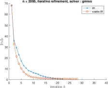
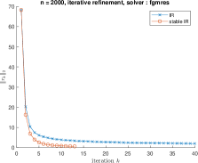
(a)                                       (b)

Fig. 1: Solving $\mathbf{A}\bm{x}=\bm{b}$ using RPU. $\mathbf{A}$ is a symmetric matrix with decreasing off-diagonal elements. (a) GMRES-IR. (b) FGMRES-IR.

 

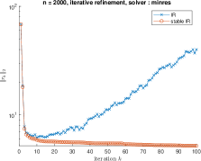
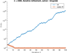
(a)                                  (b)

Fig. 2: Solving $\mathbf{A}\bm{x}=\bm{b}$ using RPU. $\mathbf{A}$ is symmetric with decreasing off-diagonal elements. (a) MINRES-IR. (b) BiCGSTAB-IR.

 

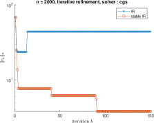
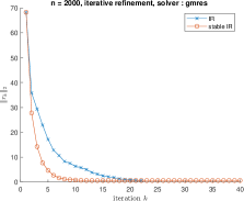
(a)                                  (b)

Fig. 3: Solving $\mathbf{A}\bm{x}=\bm{b}$ using RPU. $\mathbf{A}$ is symmetric with decreasing off-diagonal elements. (a) CGS-IR. (b) GMRES-IR running the basic method $k=10$ times between each update (Algorithm 4).

Next, we consider a different matrix $\mathbf{A}$ of size $\Mu=2000$ where each entry $[\mathbf{A}]_{ij}$ is taken i.i.d. from a uniform distribution in $[0,1]$. In this case, $\mathbf{A}$ is generally neither positive definite nor symmetric. In Fig. 4, we observe that GMRES-IR and FGMRES-IR diverge, while the stable GMRES-IR and stable FGMRES-IR algorithms do not.

 

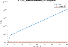
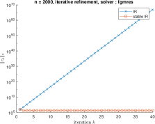
(a)                                       (b)

Fig. 4: Solving $\mathbf{A}\bm{x}=\bm{b}$ using RPU. $\mathbf{A}$ is a random $2000\times 2000$ matrix of i.i.d. entries from a uniform distribution. (a) GMRES-IR. (b) FGMRES-IR.

5.2 Low-precision digital accelerator

Our stable IR algorithms will also benefit from scenarios where the matrix-vector products during the iterative solution of the basic method are performed in lower digital precision while the rest of the steps are still performed in higher digital precision. For instance, consider the example in [32] where the basic method for solving $\mathbf{A}\bm{x}=\bm{b}$ is LU decomposition in single precision, single precision is used to store intermediate results, and the residual and $\alpha_{m}$ (if applicable) are computed in double precision. For this scheme, upon adapting the code provided in [32], Fig. 5(a) shows that LU-IR diverges for both $\|\bm{x}_{m}-\bm{x}\|$ and $\|\bm{r}_{m}\|$ under a matrix $\mathbf{A}$ with ${\mathrm{cond}({\mathbf{A}})}=1.6\times 10^{11}$. On the other hand, Fig. 5(b) shows that for the stable LU-IR scheme (Algorithm 2), $\bm{x}_{m}$ are bounded and the residual errors are within the desired precision.

 

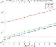
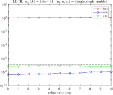
(a)                                       (b)

Fig. 5: LU-IR. ferr, nbe and cbe are the forward, normwise backward and componentwise backward error as defined in [32]. (a) IR (Algorithm 1). (b) Stable IR (Algorithm 2).

5.3 Variants of stable IR

Applying Algorithm 3 with $k=10$ to the setup in Section 5.1 shows in Fig. 6 that it performs better than Algorithm 2 with $k=1$ (Fig. 1) for both GMRES-IR and FGMRES-IR, converging to the solution in much less iterations than Algorithm 1. Similarly, for Algorithm 4 with $k=10$, we observe in Fig. 3(b) that Algorithm 4 for GMRES-IR performs better than both Algorithm 2 in Fig. 1(a) and Algorithm 3 in Fig. 6(a).

 

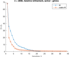
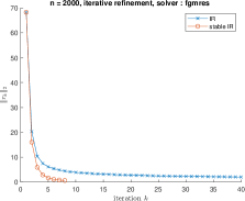
(a)                                       (b)

Fig. 6: Solving $\mathbf{A}\bm{x}=\bm{b}$ using RPU with $k=10$ previous directions. $\mathbf{A}$ is a symmetric matrix with decreasing off-diagonal elements. (a) GMRES. (b) FGMRES.

6 Conclusions

In this paper we presented a modification of the classical IR algorithm that guarantees nondivergence under unknown or arbitrarily large error for the basic method and that demonstrates performance superior to IR in practice. This is especially useful for emerging inaccurate computing paradigms where the variance of the noise/error can be unknown and/or large. One issue of the stable IR algorithm is that when $\bm{r}_{m}$ is nearly orthogonal to $\mathbf{A}\bm{d}_{m}$, this results in $\alpha_{m}$ being small resulting in minimal update. As part of our future work, we aim to find an alternative direction for $\bm{d}_{m}$ with which to update $\bm{x}_{m}$.

References

- [1] I. Markovsky and S. Van Huffel, “Overview of total least-squares methods,” Signal processing, vol. 87, no. 10, pp. 2283–2302, 2007.
- [2] J. A. Cadzow, “Signal processing via least squares error modeling,” IEEE ASSP Magazine, vol. 7, no. 4, pp. 12–31, 1990.
- [3] I. Selesnick, “Least squares with examples in signal processing,” Connexions, vol. 4, pp. 1–25, 2013.
- [4] D. Wang and F. Ding, “Least squares based and gradient based iterative identification for wiener nonlinear systems,” Signal Processing, vol. 91, no. 5, pp. 1182–1189, 2011.
- [5] K. J. Åström and P. Eykhoff, “System identification—a survey,” Automatica, vol. 7, no. 2, pp. 123–162, 1971.
- [6] L. Lu et al., “An overview of massive MIMO: Benefits and challenges,” IEEE journal of selected topics in signal processing, vol. 8, no. 5, pp. 742–758, 2014.
- [7] T. L. Marzetta, “Massive MIMO: an introduction,” Bell Labs Technical Journal, vol. 20, pp. 11–22, 2015.
- [8] E. G. Larsson, O. Edfors, F. Tufvesson, and T. L. Marzetta, “Massive mimo for next generation wireless systems,” IEEE communications magazine, vol. 52, no. 2, pp. 186–195, 2014.
- [9] Y. Saad, Iterative methods for sparse linear systems. SIAM, 2003.
- [10] M. Zhao, R. V. Panda, S. S. Sapatnekar, T. Edwards, R. Chaudhry, and D. Blaauw, “Hierarchical analysis of power distribution networks,” in Proceedings of the 37th Annual Design Automation Conference, 2000, pp. 150–155.
- [11] P. S. Chang and A. N. Willson, “Analysis of conjugate gradient algorithms for adaptive filtering,” IEEE Transactions on Signal Processing, vol. 48, no. 2, pp. 409–418, 2000.
- [12] J. Tu, M. Lou, J. Jiang, D. Shu, and G. He, “An efficient massive MIMO detector based on second-order richardson iteration: From algorithm to flexible architecture,” IEEE Transactions on Circuits and Systems I: Regular Papers, vol. 67, no. 11, pp. 4015–4028, 2020.
- [13] Z. Wang, R. M. Gower, Y. Xia, L. He, and Y. Huang, “Randomized iterative methods for low-complexity large-scale MIMO detection,” IEEE Transactions on Signal Processing, vol. 70, pp. 2934–2949, 2022.
- [14] J. Liesen and Z. Strakos, Krylov subspace methods: principles and analysis. Numerical Mathematics and Scie, 2013.
- [15] J. H. Wilkinson, Rounding errors in algebraic processes. SIAM, 2023.
- [16] G. H. Golub and Q. Ye, “Inexact preconditioned conjugate gradient method with inner-outer iteration,” SIAM Journal on Scientific Computing, vol. 21, no. 4, pp. 1305–1320, 1999.
- [17] D. F. Gleich, A. P. Gray, C. Greif, and T. Lau, “An inner-outer iteration for computing pagerank,” SIAM Journal on Scientific Computing, vol. 32, no. 1, pp. 349–371, 2010.
- [18] A. Haidar, P. Wu, S. Tomov, and J. Dongarra, “Investigating half precision arithmetic to accelerate dense linear system solvers,” in Proceedings of the 8th workshop on latest advances in scalable algorithms for large-scale systems, 2017, pp. 1–8.
- [19] C. B. Moler, “Iterative refinement in floating point,” Journal of the ACM (JACM), vol. 14, no. 2, pp. 316–321, 1967.
- [20] A. Haidar, S. Tomov, J. Dongarra, and N. J. Higham, “Harnessing gpu tensor cores for fast fp16 arithmetic to speed up mixed-precision iterative refinement solvers,” in SC18: International Conference for High Performance Computing, Networking, Storage and Analysis. IEEE, 2018, pp. 603–613.
- [21] A. Haidar, H. Bayraktar, S. Tomov, J. Dongarra, and N. J. Higham, “Mixed-precision iterative refinement using tensor cores on gpus to accelerate solution of linear systems,” Proceedings of the Royal Society A, vol. 476, no. 2243, p. 20200110, 2020.
- [22] A. Haidar et al., “The design of fast and energy-efficient linear solvers: On the potential of half-precision arithmetic and iterative refinement techniques,” in International conference on computational science. Springer, 2018, pp. 586–600.
- [23] V. Kalantzis et al., “Solving sparse linear systems with approximate inverse preconditioners on analog devices,” in 2021 IEEE High Performance Extreme Computing Conference (HPEC). IEEE, 2021, pp. 1–7.
- [24] ——, “Solving sparse linear systems via flexible GMRES with in-memory analog preconditioning,” in 2023 IEEE High Performance Extreme Computing Conference (HPEC). IEEE, 2023.
- [25] A. Alaghi and J. P. Hayes, “Survey of stochastic computing,” ACM Trans. Embed. Comput. Syst., vol. 12, no. 2s, may 2013. [Online]. Available: https://doi.org/10.1145/2465787.2465794
- [26] C. Wu, “Dither computing: a hybrid deterministic-stochastic computing framework,” in 2021 IEEE 28th Symposium on Computer Arithmetic (ARITH), 2021, pp. 70–77.
- [27] M. J. Rasch, D. Moreda, T. Gokmen, M. L. Gallo, F. Carta, C. Goldberg, K. E. Maghraoui, A. Sebastian, and V. Narayanan, “A flexible and fast pytorch toolkit for simulating training and inference on analog crossbar arrays,” arXiv preprint arXiv:2104.02184, 2021.
- [28] T. Gokmen and Y. Vlasov, “Acceleration of deep neural network training with resistive cross-point devices: Design considerations,” Frontiers in Neuroscience, vol. 10, 2016.
- [29] M. Le Gallo et al., “Mixed-precision in-memory computing,” Nature Electronics, vol. 1, no. 4, pp. 246–253, 2018.
- [30] “Accelerating data uncertainty quantification by solving linear systems with multiple right-hand sides,” Numerical Algorithms, vol. 62, pp. 637–653, 2013.
- [31] V. Kalantzis, A. C. I. Malossi, C. Bekas, A. Curioni, E. Gallopoulos, and Y. Saad, “A scalable iterative dense linear system solver for multiple right-hand sides in data analytics,” Parallel Computing, vol. 74, pp. 136–153, 2018.
- [32] E. Carson and N. J. Higham, “Accelerating the solution of linear systems by iterative refinement in three precisions,” SIAM Journal on Scientific Computing, vol. 40, no. 2, pp. A817–A847, 2018.