Improved Distributed Algorithms for Random Colorings

Abstract

Markov Chain Monte Carlo (MCMC) algorithms are a widely-used algorithmic tool for sampling from high-dimensional distributions, a notable example is the equilibirum distribution of graphical models. The Glauber dynamics, also known as the Gibbs sampler, is the simplest example of an MCMC algorithm; the transitions of the chain update the configuration at a randomly chosen coordinate at each step. Several works have studied distributed versions of the Glauber dynamics and we extend these efforts to a more general family of Markov chains. An important combinatorial problem in the study of MCMC algorithms is random colorings. Given a graph $G$ of maximum degree $\Delta$ and an integer $k\geq\Delta+1$, the goal is to generate a random proper vertex $k$-coloring of $G$.

Jerrum (1995) proved that the Glauber dynamics has $O(n\log{n})$ mixing time when $k>2\Delta$. Fischer and Ghaffari (2018), and independently Feng, Hayes, and Yin (2018), presented a parallel and distributed version of the Glauber dynamics which converges in $O(\log{n})$ rounds for $k>(2+\varepsilon)\Delta$ for any $\varepsilon>0$. We improve this result to $k>(11/6-\delta)\Delta$ for a fixed $\delta>0$. This matches the state of the art for randomly sampling colorings of general graphs in the sequential setting. Whereas previous works focused on distributed variants of the Glauber dynamics, our work presents a parallel and distributed version of the more general flip dynamics presented by Vigoda (2000) (and refined by Chen, Delcourt, Moitra, Perarnau, and Postle (2019)), which recolors local maximal two-colored components in each step.

1 Introduction

This paper presents parallel and distributed algorithms for sampling from high-dimensional distributions. An important application is sampling from the equilibrium distribution of a graphical model. The equilibrium distribution is often known as the Gibbs or Boltzmann distribution, and efficient sampling from the Gibbs/Boltzmann distribution is a key step for Bayesian inference [24, 28].

Our focus is algorithms in the LOCAL model for the $k$-colorings problem. The $k$-colorings problem is a graphical model of particular combinatorial interest and has played an important role in the development of algorithmic sampling techniques with provable guarantees. The LOCAL model is a standard model of distributed computation due to Linial [26].

In the LOCAL model, the input to a problem is generally a graph $G=(V,E)$. Each vertex is identified with a processor and is assigned a unique identifier. In each round of an algorithm, each vertex is allowed to send an unbounded amount of information (a message) to each of its neighbors, and may perform an unbounded amount of computation locally.

For an input graph $G=(V,E)$ and integer $k\geq 2$, let $\Omega$ denote the proper (vertex) $k$-colorings of $G$, namely $\Omega=\{\sigma:V\rightarrow\{1,\dots,k\}:\mbox{ for all }(v,w)\in E,\sigma(v)\neq\sigma(w)\}$ is the collection of assignments of $k$ colors to the vertices so that neighboring vertices receive different colors. The associated Gibbs distribution $\mu$ is the uniform distribution over $\Omega$, the space of proper $k$-colorings.

Under mild conditions on $G$ (e.g., triangle-free [3]), the number of $k$-colorings is exponentially large, i.e., $|\Omega|=\exp(\Omega(n))$. Nevertheless, our goal is to sample from $\mu$, the uniform distribution over this exponentially large set, in time $\mathrm{poly}(n)$, and ideally in time $O(n\log{n})$. Furthermore, in the distributed setting our goal is to generate samples ideally in time $O(\log{n})$.

A common technique for sampling from the Gibbs distribution in a wide range of scientific fields is the Markov Chain Monte Carlo (MCMC) method. The simplest example of an MCMC algorithm is the Glauber dynamics, also known as the Gibbs sampler.

Consider an input graph $G=(V,E)$ with maximum degree $\Delta$, and $k\geq\Delta+2$. The Glauber dynamics updates the color of a randomly chosen vertex in each step. In particular, from a coloring $X_{t}\in\Omega$ at time $t$, the transitions $X_{t}\rightarrow X_{t+1}$ of the Glauber dynamics work as follows. We choose a random vertex $v$ uniformly at random from $V$, and a color $c$ uniformly at random from the set of colors $\{1,\dots,k\}$. If no neighbor of $v$ has color $c$ in the current coloring $X_{t}$, i.e., $c\not\in X_{t}(N(v))$ where $N(v)$ are the neighbors of vertex $v$, then we recolor $v$ as $X_{t+1}(v)=c$ and otherwise we set $X_{t+1}(v)=X_{t}(v)$. For all other vertices $w\neq v$ we set $X_{t+1}(w)=X_{t}(w)$. This corresponds to the Metropolis version of the Glauber dynamics. Alternatively one can choose the color $c$ uniformly from $\{1,\dots,k\}\setminus X_{t}(N(v))$, which is the set of colors that do not appear in the neighborhood of $v$ in $X_{t}$; this is the heat-bath version of the Glauber dynamics.

When $k\geq\Delta+2$ then the Glauber dynamics is ergodic and the unique stationary distribution is uniform over $\Omega$. The mixing time is the number of steps, from the worst initial state $X_{0}$, so that the chain is within total variation distance $\leq 1/4$ of the stationary distribution (see Section 2.2) for a more formal definition.

There are various attempts at running asynchronous versions of the Glauber dynamics in the distributed setting, namely HOGWILD! [35, 40], but there are few theoretical results and the resulting process is not guaranteed to have the correct asymptotic distribution [8, 7, 36]. There is also considerable work in constructing distributed sampling algorithms, including distributed versions of the Glauber dynamics [14, 13, 22, 12, 11, 27]; we discuss below the relevant results in our setting of the colorings problem. An important caveat about previous results is that they require a strong form of decay of correlations, such as the Dobrushin uniqueness condition, and our results hold in regions where Dobrushin’s uniqueness condition does not hold.

In the sequential setting, a seminal work of Jerrum [21] proved $O(n\log{n})$ mixing time of the Glauber dynamics whenever $k>2\Delta$ where $\Delta$ is the maximum degree. Vigoda [37] presented an alternative dynamics which we will refer to as the flip dynamics and proved $O(n\log{n})$ mixing time of the flip dynamics when $k>\frac{11}{6}\Delta$. The flip dynamics is a generalization of the Glauber dynamics which “flips” maximal 2-colored components (clusters) in each step by interchanging the pair of colors on the chosen cluster; Vigoda’s analysis chooses particular flip probabilities which depend on the size of the chosen cluster and do not flip any cluster larger than size six.

Vigoda’s result was recently improved to $k>(\frac{11}{6}-\varepsilon_{0})\Delta$ for some fixed $\varepsilon_{0}\approx 10^{-5}$ by Chen, Delcourt, Moitra, Perarnau, and Postle [5]. This later result of $k>(\frac{11}{6}-\varepsilon_{0})\Delta$ is the best known result for general graphs. There are various improvements (e.g., [9, 6]), however they all require particular girth or maximum degree assumptions; the girth is the length of the shortest cycle.

In the distributed setting, Feng, Sun and Yin [12] achieved $O(\Delta\log{n})$ rounds in LOCAL model when $k>(2+\varepsilon)\Delta$ and $O(\log{n})$ rounds when $k>(2+\sqrt{2})\Delta$. Fischer and Ghaffari [14], and independently, Feng, Hayes and Yin [11], presented a distributed algorithm which converges in $O(\log{n})$ rounds for $k$-colorings on any graph of maximum degree $\Delta$ when $k>(2+\varepsilon)\Delta$ for any $\varepsilon>0$. These results match Jerrum’s result (in the sequential setting) for general graphs. We improve upon these works to match the current state of the art results in the sequential setting for general graphs for $k>(11/6)\Delta$.

We present the following improved result:

Theorem 1.1.

For all $\varepsilon>0$, all $\Delta\geq 2$, all $\delta>0$, and any $k>(11/6+\varepsilon)\Delta$, for any graph $G=(V,E)$ of maximum degree $\Delta$, a random $k$-coloring within total variation distance $\leq\delta$ from uniform can be generated in $O(\log(n/\delta))$ rounds, where $n=|V|$.

The above result is optimal as there is a matching $\Omega(\log(n/\delta))$ lower bound due to Feng, Sun, and Yin [12]. Moreover, combining our analysis with the refined analysis of Chen et al. [5] we obtain the following result.

Theorem 1.2.

There exists $\varepsilon^{*}>0$, for all $\Delta\geq 2$, all $\delta>0$, and any $k>(11/6-\varepsilon^{*})\Delta$, for any graph of maximum degree $\Delta$, a random $k$-coloring within total variation distance $\leq\delta$ from uniform can be generated in $O(\log(n/\delta))$ rounds.

The Dobrushin uniqueness condition, which is a sufficient condition in several previous distributed sampling works, holds for colorings on general graphs of maximum degree $\Delta$ iff $k~{}>~{}2\Delta$ [33]. Thus, our results hold beyond the Dobrushin uniqueness threshold, and thereby resolves an open problem of [14] who asked “whether efficient distributed algorithms intrinsically need to be stuck at Dobrushin’s condition.”

Our proof of fast convergence of our new distributed flip dynamics utilizes the path coupling framework of Bubley and Dyer [4], which is an important tool in the analysis of the mixing time for sequential Markov chains. In a coupling analysis path coupling allows one to only consider “neighboring pairs”. In the special case of the Glauber dynamics, path coupling is related to Dobrushin’s uniqueness condition but path coupling is a weaker condition (namely, Dobrushin’s uniqueness condition implies path coupling). We believe our work raises the following intriguing open question. For any spin system, or equivalently any undirected graphical model, does the path coupling condition for a local (sequential) Markov chain imply the existence of an efficient distributed algorithm which converges in $O(\log{n})$ steps?

1.1 Motivation

Designing a distributed algorithm for constructing a coloring is a seminal problem in the study of distributed algorithms [26, 29]. It is an important problem in the study of symmetry breaking and is useful in the design of networking algorithms [2, 34, 25, 26]. One of the fundamental problems in this context that has received significant attention is minimizing the number of rounds required to construct a $(\Delta+1)$-coloring in the LOCAL model; see Barenboim, Elkin, and Goldenberg [1] for a recent breakthrough, and see [15, 16] for more recent follow-up works.

Our focus is on generating a random coloring, in other words to generate a sample from the uniform distribution over all colorings, or more precisely, from a distribution that is arbitrarily close (in total variation distance) from the uniform distribution. More generally, our goal is to sample from the equilibrium distribution of a graphical model.

Graphical models are a fundamental tool in machine learning [28], and the associated sampling problem is important for associated learning, inference, and testing problems. A noteworthy example in the history of graphical models and in the importance of the associated sampling problem is the work on Restricted Boltzmann Machines (RBMs) of Hinton [18]. An RBM is an instance of the Ising model on a bipartite graph. The Ising model is a simpler variant of the random colorings problem in which we are sampling labellings of the vertices of a bipartite graph with only 2 colors where the labellings are weighted exponentially by the number of monochromatic edges; the generalization to $k>2$ colors is the Potts model, and the zero-temperature (antiferromagnetic) Potts model is the random colorings problem that we study. The design of fast learning algorithms for RBMs was fundamental in the development of deep learning algorithms [19, 20, 30, 31, 32].

Given the proliferation of machine learning tasks on high-dimensional data, there is a clear need for distributed sampling algorithms for graphical models. For example, speeding up inference in latent Dirichlet allocation models via parallel and distributed Gibbs sampling [38, 23] and via the stochastic gradient sampler [39] has received attention in the machine learning community, as has the distributed problem of finding a $k$-coloring as a subroutine for Gibbs sampling [17].

Sampling colorings is a natural combinatorial problem to address particularly because of its importance in the study of sequential sampling algorithms. Jerrum’s sampling algorithm [21] for $k>2\Delta$ colors was a seminal work as it pioneered the use of the coupling method for sampling problems on graphical models. As mentioned earlier, Vigoda [37] improved Jerrum’s result to $k>11\Delta/6$ and this was the state of the art until the recent improvement to $k>(11/6-\varepsilon)\Delta$ [5]. One of the major open problems in the area of sequential sampling is to obtain an efficient sampling scheme when $k>\Delta+1$, see [6] for the most recent progress.

Our general question is whether efficient sequential sampling schemes yield efficient distributed sampling algorithms, by which we mean an $O(\log{n})$ round algorithm in the LOCAL model. A distributed version of the Metropolis version of the Glauber dynamics for colorings was introduced in [14, 11] and was proved to be an efficient distributed sampling scheme when $k>(2+\varepsilon)\Delta$ for all $\varepsilon>0$. Our work goes beyond the single-site Glauber dynamics to designing efficient distributed sampling schemes for more general dynamics.

1.2 Technical Contribution

Recall that the Glauber dynamics updates a single vertex in each step. Several recent works present and analyze distributed versions of the Glauber dynamics (specifically, the Metropolis version) in various contexts [14, 11, 27, 12]. For more general MCMC algorithms which update larger regions than a vertex in each step, do efficient convergence results in the sequential setting for such Markov chains yield efficient distributed sampling algorithms?

A prime example to consider for this more general question is Vigoda’s flip dynamics [37]. Attaining a distributed version of the flip dynamics is more challenging as we need to simultaneously recolor clusters of up to 6 vertices; here a cluster refers to a maximal 2-colored component and the recoloring acts by interchanging the respective pair of colors on each cluster. Our first contribution is presenting a distributed version of Vigoda’s flip dynamics. The challenge is to make a distributed version which is efficient but simple enough that we can still analyze it.

To parallelize the cluster recolorings, we need to ensure that no two overlapping clusters are simultaneously active, and that no two neighboring clusters that share colors are both active. On the other hand, we need to “activate” each cluster for potential recoloring with a sufficiently large probability to obtain a mixing time that is independent of the maximum degree, namely $O(\log{n})$.

Our analysis of our distributed version of Vigoda’s flip dynamics follows the high-level coupling presented in Vigoda’s original work [37]. A coupling analysis of a Markov chain, considers two copies of the Markov chain (in this case the distributed flip dynamics), each with arbitrary starting states. Our aim is that there are “coupled transitions” for the two chains so that after $O(\log{n})$ steps the two chains have coalesced in the same state with sufficiently large probability; by coupled transition we mean that the two chains can couple their transitions as long as when viewed in isolation, each is a faithful copy of the original Markov chain. The idea is that if we consider one of the chains to be in the stationary distribution, then we showed that after $O(\log{n})$ steps our algorithm has likely reached the stationary distribution and hence the mixing time is $O(\log{n})$.

There are several important technical challenges that arise when doing a coupling analysis in the distributed setting for the flip dynamics. First, we need to ensure that the clusters we flip (which means swap the pair of colors in a maximal 2-colored component) do not interfere with any other clusters we might flip by either overlapping, or by neighboring and containing a common color. Subsequently when we do try to couple a pair of flips in the two coupled chains, we need to consider the case that one of these two clusters is not flippable in only one chain due to one of these aforementioned conflicts (such as an overlapping cluster in only one of the chains).

Finally, we use the path coupling framework [4] which allows us to restrict attention to the case that the pair of coupled chains only differ at a single vertex $v^{*}$; this was crucial in Vigoda’s original analysis as well. Vigoda’s analysis only needed to consider clusters that include $v^{*}$ or that neighbor this disagree vertex $v^{*}$. In our setting we also need to analyze and couple clusters that are distance 2 away from $v^{*}$, where distance is measured by cluster flips; this is due to a neighboring cluster possibly being flippable in only one of the chains and then this effect reverbates out. Moreover, those coupling for clusters at distance $<2$ from $v^{*}$ is more complicated than the sequential setting as a coupled cluster might not be flippable in only one chain due to conflicts with other clusters.

Our work suggests that a more general phenomenon is at play. We conjecture that, for any graphical model, a path coupling analysis for any local Markov chain in the sequential setting yields an efficient distributed sampling scheme. We believe our work will be an important step towards proving this general conjecture.

1.3 Paper Overview

In Section 3, we present a parallel and distributed version of Vigoda’s flip dynamics. We analyze the mixing time of our distributed flip dynamics when $k>(11/6+\varepsilon)\Delta$ for any $\varepsilon>0$, thereby proving Theorem 1.1, in Sections 4 and 5. We use a coupling argument that builds upon the analysis in Vigoda [37]. Our analysis is more complicated than the original argument of Vigoda due to clusters which appear in both coupled chains, but possibly being “flippable” in one chain but not the other chain due to differing conflicts with neighboring clusters, see Section 1.2 for a very high-level overview. Finally, in Appendix B, we further utilize the linear programming (LP) framework and the refined metric on colorings presented in Chen et al. [5] to achieve the further improved result as stated in Theorem 1.2. This proof combines our proof approach for Theorem 1.1 with the more technical analysis of Chen et al. [5].

2 Preliminaries

Let $[k]=\{1,\dots,k\}$. For a graph $G=(V,E)$ let $i\sim j$ denote $(i,j)\in E$, and for $v\in V$, let $N(v)=\{w\in V:v\sim w\}$ denote the neighbors of a vertex $v$. For integer $k\geq 2$, let $\Omega^{*}=[k]^{V}$ denote the set of $k$-labellings and $\Omega=\{\sigma\in[k]^{V}:\mbox{for all }i\sim j,\sigma(i)\neq\sigma(j)\}$ denote the set of $k$-colorings of $G$. Throughout this paper, a coloring (or $k$-coloring) refers to a proper vertex $k$-coloring.

2.1 Clusters

For a coloring $\sigma$, a cluster $S$ in $\sigma$ is a maximal 2-colored component of size at most 6; this is formally defined in the following definition.

Definition 2.1.

Let $G=(V,E)$ be a graph and $\sigma\in\Omega^{*}$. For a vertex $v\in V$ and color $c\in[k]$ let $S_{\sigma}(v,c)$ denote the set of vertices reachable from $v$ by a $(\sigma(v),c)$ alternating path. When $|S_{\sigma}(v,c)|\leq 6$ then we refer to $S=S_{\sigma}(v,c)$ as a cluster. Let

$$\SS_{\sigma}=\bigcup_{v\in V,c\in[k]}\{S_{\sigma}(v,c):|S_{\sigma}(v,c)|\leq 6\},$$

denote the collection of all clusters in $\sigma$ of size at most 6, where the size of a cluster refers to the number of vertices in the cluster. The restriction to size at most 6 is due to the Markov chain used as in previous works [37, 5].

For a labelling $\sigma\in\Omega^{*}$, vertex $v\in V$, and color $c\in[k]$, the flip of cluster $S_{\sigma}(v,c)$ interchanges colors $\sigma(v)$ and $c$ on the set $S_{\sigma}(v,c)$. Let $\sigma^{\prime}$ denote the resulting coloring after this flip of cluster $S_{\sigma}(v,c)$. Notice that if $\sigma\in\Omega$ then $\sigma^{\prime}\in\Omega$, i.e., if it is a proper coloring before the flip, then after the flip it remains a proper coloring since the clusters are maximal 2-colored components. This is the key property for the flip dynamics as once we reach a proper coloring then we are guaranteed to stay at proper colorings. Nevertheless, the definition of a cluster $S_{\sigma}(v,c)$ is also defined for improper colorings $\sigma\in\Omega^{*}\setminus\Omega$; this enlarged state space of improper colorings is used in the proof but not in the algorithm itself, see Section 4.2 for further discussion of this technicality.

Consider a coloring $\sigma\in\Omega$ and a vertex $v\in V$. For every color $c$ which does not appear in the neighborhood of $v$, i.e., $c\not\in\sigma(N(v))$ then the corresponding cluster is of size 1, i.e., $|S_{\sigma}(v,c)|=1$ since $S_{\sigma}(v,c)=\{v\}$. Flips of these singleton clusters are exactly the transitions of the Glauber dynamics. The flip dynamics of Vigoda [37] is a generalization of the Glauber dynamics in which clusters of size at most 6 are flipped with positive probability (depending on the size of the cluster). Note, for $c=\sigma(v)$ then we get a singleton cluster and the flip does not change the coloring, hence the flip dynamics has a non-zero self-loop probability and thus is aperiodic.

For clusters $S,T\in\SS_{\sigma}$, we say $S$ and $T$ are neighboring clusters, which we denote as $S\sim T$, if there exists $v\in S$ and $w\in T$ where $v\sim w$.

2.2 Markov Chains

Consider a Markov chain $(X_{t})$ with state space $\Omega$ and transition matrix $P$ and unique stationary distribution $\pi$. We say that the chain is aperiodic if $\gcd\{t\colon P^{t}(x,x)>0\}=1$ for all $x\in\Omega$ and irreducible if for all $x,y\in\Omega$, there exists a $t$ such that $P^{t}(x,y)>0$. Recall that if the chain is both aperiodic and irreducible, then it is ergodic and the chain has a unique stationary distribution $\pi$ where: $\text{for all }x,y\in\Omega,\lim_{t\rightarrow\infty}P^{t}(x,y)=\pi(y).$ If $P$ is symmetric, then $\pi$ is the uniform distribution over $\Omega$.

The mixing time is the number of steps, from the worst initial state $X_{0}$, until the chain is within total variation distance $\leq 1/4$ of the stationary distribution:

$$T_{\mathrm{mix}}:=\max_{x\in\Omega}\min\{t\mid\|P^{t}(\sigma,\cdot)-\mu\|_{\rm TV}\leq 1/4\},$$

where $d_{TV}$ is the total variation distance, $\|\mu-\omega\|_{\rm TV}:=\frac{1}{2}\sum_{x\in\Omega}\lvert\mu(x)-\omega(x)\rvert.$ The choice of constant $1/4$ is somewhat arbitrary since, for any $\varepsilon>0$, we can obtain total variation distance $\leq\varepsilon$ after $\leq\log(1/\varepsilon)T_{\mathrm{mix}}$ steps.

2.3 Path Coupling

Consider an ergodic Markov chain $\mathcal{MC}$ with state space $\Omega$ and transition matrix $P$. A coupling for $\mathcal{MC}$ defines, for all pairs $X_{t},Y_{t}\in\Omega$, a joint transition $(X_{t},Y_{t})\rightarrow(X_{t+1},Y_{t+1})$ such that the individual transitions $(X_{t}\rightarrow X_{t+1})$ and $(Y_{t}\rightarrow Y_{t+1})$, when viewed in isolation from each other, act according to the transition matrix $P$. The goal is to find a coupling that minimizes the coupling time: $T_{\mathrm{couple}}:=\min\left\{t\mid\mbox{ for all }X_{0},Y_{0}\in\Omega,{\mathbf{Pr}\left({X_{t}\neq Y_{t}}\mid{X_{0},Y_{0}}\right)}\leq 1/4\right\}.$ This implies that $T_{\mathrm{mix}}\leq T_{\mathrm{couple}}$.

To bound the coupling time and hence the mixing time, we use the use the path coupling method of Bubley and Dyer [4] which allows us to only consider a small subset of pairs of states. We will analyze the coupling with respect to the Hamming distance $H(\sigma,\tau):=\sum_{v\in V}\mathbf{1}(\sigma(v)\not=\tau(v))$. We present the more general form of path coupling in Section B.1 which allows more general metrics.

Theorem 2.2.

[4, 10] Consider an ergodic Markov chain on $\Omega^{*}=[k]^{V}$. Let $\beta>0$. If for all pairs of states $X_{t},Y_{t}\in\Omega^{*}$ where $H(X_{t},Y_{t})=1$, there exists a coupling such that:

$${\mathbf{E}\left({H(X_{t+1},Y_{t+1})}\mid{X_{t},Y_{t}}\right)}\leq(1-\beta)H(X_{t},Y_{t}),$$

then the mixing time is bounded by $T_{mix}\leq O\left(\frac{\log(|V|)}{\beta}\right).$ Moreover, the mixing time within total variation distance $\leq\delta$, for any $\delta>0$, in time $O(\log(|V|)/(\beta\delta))$.

3 Algorithm Description: Distributed Flip Dynamics

We begin by defining a sequential process and then show that this process can be implemented efficiently in a distributed manner.

We have the following parameters in our algorithm. Let $\alpha=\varepsilon/(5000k)$ where $k\geq(11/6+\varepsilon)\Delta$ for some $\varepsilon>0$. The parameter $\alpha$ will be used for the activation probability of a cluster. In Appendix B when we strengthen the main result for $k<(11/6)\Delta$ then we will redefine $\alpha$ so that it depends on the distance of $k$ below $(11/6)\Delta$.

Let $1\geq f_{i}\geq 0$ for all $i\geq 1$ be a sequence of “flip” probabilities that contain the following key properties: $f_{1}=1$, $f_{i}\geq f_{i+1}$ for all $i$, and $f_{i}=0$ for all $i\geq 7$. The following process is well-defined for any choice of flip probabilities with these properties. To prove Theorems 1.1 and 1.2 we will choose slightly different flip probabilities. In particular, to prove the slightly weaker result (Theorem 1.1) in Section 4 we will choose flip probabilities as in [37], and then to get the refined result (Theorem 1.2) in Appendix B we will use the setting in [5].

We now define the Markov chain $\mathcal{MC}_{\mathrm{flip}}$ with state space $\Omega$. For a coloring $X_{t}\in\Omega$, the transitions $X_{t}\rightarrow X_{t+1}$ of $\mathcal{MC}_{\mathrm{flip}}$ are defined as follows:

1. Independently for each $S\in\SS_{\sigma}$, cluster $S$ is active with probability $\alpha$.

2. A cluster $S=S_{X_{t}}(v,c)$ is flippable if the following hold:

   1. $S$ is active;

   2. Overlapping clusters: There is no active $S^{\prime}\neq S$ where $S\cap S^{\prime}\neq\emptyset$;

   3. Conflicting neighboring clusters: For all active clusters $T=T_{X_{t}}(w,c^{\prime})$ where $S\sim T$, $\{X_{t}(v),c\}\cap\{X_{t}(w),c^{\prime}\}=\emptyset$.

3. Independently for each flippable cluster $S$, flip $S$ with probability $f_{i}$ where $i=|S|$.

4. Let $X_{t+1}$ denote the resulting coloring.

Notice that step 2c is saying that for a pair of active and neighboring clusters $S$ and $T$, the pair of colors defining cluster $S$ are disjoint from the pair of colors defining cluster $T$.

Lemma 3.1.

The Markov chain $\mathcal{MC}_{\mathrm{flip}}$ is ergodic and symmetric and hence the unique stationary distribution is the uniform distribution over $\Omega$.

Proof.

Observe that with positive probability, no cluster is active and $P(\sigma,\sigma)>0$ for all $\sigma\in\Omega$. Thus, the Markov chain is aperiodic. For irreducibility, since $f_{1}>0$, the irreducibility of $\mathcal{MC}_{\mathrm{flip}}$ follows from irreducibility of the Glauber dynamics which holds whenever $k\geq\Delta+2$ (see, e.g., Jerrum [21]). Hence, the chain is ergodic. Moreover, the chain is symmetric, for $\sigma\in\Omega$, let $\sigma^{\prime}$ be the coloring obtained from $\sigma$ after flipping clusters $S_{\sigma}(v_{1},c_{1}),\dots,S_{\sigma}(v_{\ell},c_{\ell})$ in one step of $\mathcal{MC}_{\mathrm{flip}}$. Then, starting from $\sigma^{\prime}$ and flipping clusters $S_{\sigma^{\prime}}(v_{1},\sigma(v_{1})),\dots,S_{\sigma^{\prime}}(v_{\ell},\sigma(v_{\ell}))$ recovers $\sigma$. Since $\mathcal{MC}_{\mathrm{flip}}$ is ergodic and symmetric then the uniform distribution is the unique stationary distribution. ∎

Lemma 3.2.

Each step of the Markov chain $\mathcal{MC}_{\mathrm{flip}}$ can be implemented in the LOCAL model in $O(1)$ rounds.

Proof.

We describe the steps of the algorithm and how to implement them in the LOCAL model. At a given time step $t$, denote the current coloring as $\sigma=X_{t}$.

1. For each vertex $v\in V$ and for each color $c\in[k]$, identify the cluster $S_{\sigma}(v,c)$. We accomplish this step by (i) sending a message indicating the index of $v$ to each neighboring vertex $w$ with $\sigma(w)=c$, (ii) passing this message, along with the index of $w$, to each neighbor $x$ of $w$ with $\sigma(x)=\sigma(v)$, and (iii) repeating this process for up to six rounds. After the six rounds, each vertex has received the identities of all other vertices in its six-hop neighborhood with which it might share a cluster, and thus can determine the clusters (and their sizes) to which it belongs. Moreover, any 2-colored components of size $>6$ will be identified and discarded.

2. Fix an arbitrary ordering of the vertex set of $G$ and for each cluster $S$, identify $\operatorname{pres}(S)$, the lowest-index vertex $v\in S$. We can accomplish this step by letting each vertex $u\in S$ compare its own index to each of the indices of other vertices in $S$, which have been passed during step 1.

3. For each cluster $S$, activate $S$ with probability $\alpha$. More precisely, for each $v\in V$ and for each $c\in[k]$, if $v=\operatorname{pres}(S_{\sigma}(v,c))$, activate $S_{\sigma}(v,c)$ by sending a message to every $u\in S_{\sigma}(v,c)$.

4. Detect conflicts:

   1. Overlapping clusters: For all $v\in V$, if $S_{\sigma}(v,c),S_{\sigma}(v,c^{\prime})$ are both active for some $c\neq c^{\prime}$, send messages to $\operatorname{pres}(S_{\sigma}(v,c)),\operatorname{pres}(S_{\sigma}(v,c^{\prime}))$ to “deactivate” $S_{\sigma}(v,c),S_{\sigma}(v,c^{\prime})$.

   2. Conflicting neighboring clusters: For all $v\in V$, for every neighbor $w$ of $v$, if there exist clusters $S_{\sigma}(v,c)\neq S_{\sigma}(w,c^{\prime})$ such that $\{\sigma(v),c\}\cap\{\sigma(w),c^{\prime}\}\neq\emptyset$ and if $S_{\sigma}(v,c)$ and $S_{\sigma}(w,c^{\prime})$ are both active, deactivate $S_{\sigma}(v,c)$ and $S_{\sigma}(w,c)$ (by sending messages to $\operatorname{pres}(S_{\sigma}(v,c))$ and $\operatorname{pres}(S_{\sigma}(w,c))$).

5. For all $v\in V$, for all $c\in[k]$, if $S_{\sigma}(v,c)$ is still active and $v=\operatorname{pres}(S_{\sigma}(v,c))$, flip $S_{\sigma}(v,c)$ with probability $f_{i},$ where $i=|S_{\sigma}(v,c)|$ (by sending a message to each $w\in S_{\sigma}(v,c)$ to change its color from $c$ to $\sigma(v)$ or vice versa).

Since, in step 5, only $\operatorname{pres}(S)$ is responsible for flipping $S$, the probability of a given cluster $S$ being flipped, conditioned on $S$ being active and having no active neighboring or overlapping cluster, is $f_{|S|}$.

Each of the above steps requires a constant number of rounds, proving the claim. Furthermore, the amount of computation performed locally at each vertex depends only (and polynomially) on the maximum degree of the graph and the number of colors. That is, not only is the number of rounds in the LOCAL model $O(1)$, but also the algorithm is efficient with respect to the local computation performed in each round. ∎

4 Analysis of Distributed Flip Dynamics

Here we prove our main result Theorem 1.1, namely fast convergence of the distributed flip dynamics when $k>(11/6+\varepsilon)\Delta$ for any $\varepsilon>0$. Hence, fix $\varepsilon>0$ and $k>(11/6+\varepsilon)\Delta$. Our specific choice of flip probabilities for this section and for Section 5 are the following:

$$f_{1}=1,\ f_{2}=13/42,\ f_{3}=1/6,\ f_{4}=2/21,\ f_{5}=1/21,\ f_{6}=1/84.$$ (1)

These parameters match the original paper of Vigoda [37]; there are other parameter choices for which the analysis works, e.g., see [5], in fact, we will utilize these alternative parameters in Appendix B.

4.1 Overview

We will analyze the mixing time of the chain $\mathcal{MC}_{\mathrm{flip}}$ using path coupling. Consider a pair of colorings $X_{t},Y_{t}$ which differ at exactly one vertex and let $v^{*}$ denote the disagreement, i.e., $X_{t}(v^{*})\neq Y_{t}(v^{*})$ and for all $w\neq v^{*}$, $X_{t}(w)=Y_{t}(w)$. Our coupling is the identity coupling for all clusters that are the same in both chains, i.e., for all clusters $S$ where $S=S_{X_{t}}(w,c)=S_{Y_{t}}(w,c)$ for some $w\in V,c\in[k]$, we use the identity coupling for the activation probability. By the identity coupling for the activation probability we mean that with probability $\alpha$ the cluster $S$ is active in both chains, and with probability $1-\alpha$ it is inactive in both chains. Moreover, if the cluster $S$ is flippable in both chains then we also use the identity coupling for the flip probability, which means that if both clusters are flippable then with probability $\alpha$ we flip the cluster in both chains and with probability $1-\alpha$ we flip the cluster in neither of the chains.

We will define the distance of cluster $T$ from the disagree vertex $v^{*}$ based on the shortest path via neighboring clusters.

Definition 4.1.

For a coloring $\sigma\in\{X_{t},Y_{t}\}$, and a cluster $T\in\SS_{\sigma}$, we define $\mathrm{dist}(v^{*},T)$ inductively as follows. If $T=\{v^{*}\}$ then let $\mathrm{dist}_{\sigma}(v^{*},T)=0$. In general, let

$$\mathrm{dist}_{\sigma}(v^{*},T)=\min\{i:\mbox{there exists }S\in\SS_{\sigma}\mbox{ where }S\sim T,\mathrm{dist}_{\sigma}(v^{*},S)=i-1\}.$$

Remark 4.2.

Note, this notion of distance is equivalent to the shortest path distance from the singleton cluster $\{v^{*}\}$ in the cluster graph; the cluster graph is the graph on all clusters in coloring $\sigma$ where clusters $S$ and $T$ are adjacent if $S\sim T$. Distance $0$ clusters are the singleton sets $\{v^{*}\}$ for every color which does not appear in the neighborhood of $v^{*}$. Distance $1$ clusters are those that contain a neighbor of $v^{*}$ (regardless of whether they also contain $v^{*}$).

Any clusters $T$ where no vertex in $T$ is adjacent to $v^{*}$ are identical in the two chains, and thus, for every $i\geq 2$:

$$T\in\SS_{X_{t}},\mathrm{dist}_{X_{t}}(v^{*},T)=i\iff T\in\SS_{Y_{t}},\mathrm{dist}_{Y_{t}}(v^{*},T)=i.$$

Similarly, the only clusters $T$ which “disagree” in the sense that they appear in only one chain then $T$ is at distance $1$ from $v^{*}$; more formally, if $T\in\SS_{X_{t}}\setminus\SS_{Y_{t}}$, then $\mathrm{dist}_{X_{t}}(v^{*},T)=1$, and if $T\in\SS_{Y_{t}}\setminus\SS_{X_{t}}$, then $\mathrm{dist}_{Y_{t}}(v^{*},T)=1$. We use $\mathrm{dist}(v^{*},T)$ when the distances are equal, i.e., $\mathrm{dist}_{X_{t}}(v^{*},T)=\mathrm{dist}_{Y_{t}}(v^{*},T)$.

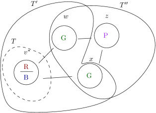
Figure 1: The vertex $v$ has $X_{t}(v)=R$ and $Y_{t}(v)=B$. Here, $T=S_{\sigma}(v,R)=S_{\tau}(v,B),$ where $\sigma=X_{t}$ and $\tau=Y_{t}$. By Definition 4.1, $\mathrm{dist}(v^{*},T)=0,\mathrm{dist}(v^{*},T^{\prime})=\mathrm{dist}(v^{*},T^{\prime\prime})=1$.

For such clusters $T$ where $\mathrm{dist}(v^{*},T)\geq 2$ we use the identity coupling for the activation probability in $X_{t}$ and $Y_{t}$, and thus the cluster $T$ is active in both chains or in neither chain. It follows that for clusters $T^{\prime}$ with $\mathrm{dist}(v^{*},T^{\prime})\geq 3$ then the cluster is flippable in both chains or in neither chain, as their neighboring active clusters are identical in the two chains. Therefore, we can use the identity coupling for the flip probability of this cluster $T$ if the cluster is flippable, and such clusters are flipped in both chains or neither chain; this leads to the following observation.

Observation 4.3.

For any cluster $T^{\prime}$ where $\mathrm{dist}(v^{*},T^{\prime})\geq 3$, $X_{t+1}(T^{\prime})=Y_{t+1}(T^{\prime}).$

For clusters $T$ where $\mathrm{dist}_{G}(T,v^{*})=2$, it can occur that $T$ is flippable in only one of the chains (due to a neighboring cluster at distance $1$ that occurs in only one of the chains). Hence, there is a probability that such clusters can be a new disagreement. The upcoming Lemma 4.4 proves that this occurs with an arbitrarily small constant probability.

The following lemma bounds the expected increase in Hamming distance from flips on clusters at distance exactly $2$ from $v^{*}$.

Lemma 4.4.

$$\sum_{T:\mathrm{dist}(v^{*},T)=2}|T|{\mathbf{Pr}\left({X_{t+1}(T)\neq Y_{t+1}(T)}\right)}\leq\alpha\varepsilon\Delta/10,$$

where $k\geq(\frac{11}{6}+\varepsilon)\Delta$.

We will account for these potential disagreements at distance 2 via the clusters at distance 1. For a cluster $T$ at distance 1 to occur in only one of the chains, the pair of colors defining $T$ must include color $X_{t}(v^{*})$ or color $Y_{t}(v^{*})$.

Proof of Lemma 4.4.

Let $\SS_{X_{t}}\oplus\SS_{Y_{t}}:=(\SS_{X_{t}}\setminus\SS_{Y_{t}})\cup(\SS_{Y_{t}}\setminus\SS_{X_{t}})$ denote the set of clusters that appear in one chain but not in the other chain. Consider a cluster $S\in\SS_{X_{t}}\oplus\SS_{Y_{t}}$. Note, all such $S$ are at $\mathrm{dist}(v^{*},S)=1$.

Let $c_{X}=X_{t}(v^{*})$ and $c_{Y}=Y_{t}(v^{*})$. These clusters $S\in\SS_{X_{t}}\oplus\SS_{Y_{t}}$ are either:

$$S_{X_{T}}(w,c_{X}),S_{X_{T}}(w,c_{Y}),S_{Y_{T}}(w,c_{X}),\mbox{ or }S_{Y_{T}}(w,c_{Y}),$$

for some neighbor $w\in N(v^{*})$. Hence, there are $\leq 4\Delta$ such clusters $S\in\SS_{X_{t}}\oplus\SS_{Y_{t}}$.

Each such cluster $S$ has size $\leq 6$ and hence it has $\leq 6\cdot 2\Delta$ neighboring clusters $T$ that share a color with $S$. These clusters $T$ are at distance $=2$ from $v^{*}$. Note that if $S$ and $T$ are both active then $T$ is not flippable in one of the chains, but it may be flippable in the other chain where $S$ does not appear; hence, the chains $X_{t+1}$ and $Y_{t+1}$ potentially differ at $T$. This yields the following:

$$\sum_{T:\mathrm{dist}(v^{*},T)=2}|T|{\mathbf{Pr}\left({X_{t+1}(T)\neq Y_{t+1}(T)}\right)}\leq 6\times(4\Delta)(12\Delta)\alpha^{2}=288\Delta^{2}\alpha^{2}\leq\varepsilon\alpha\Delta/10.$$

∎

We now account for the “good moves” where the disagreement at $v^{*}$ is removed. This occurs by Glauber updates at $v^{*}$ where we update $v^{*}$ to an available color, which is a color that does not appear in its neighborhood.

Definition 4.5.

Denote the set of available colors for $v^{*}$ in $X_{t}$ as:

$$A(v^{*})=A_{X_{t}}(v^{*}):=\{c:c\notin X_{t}(N(v^{*}))\}.$$

Note, the sets $A_{X_{t}}(v^{*})=A_{Y_{t}}(v^{*})$ since $v^{*}$ is the only disagreement at time $t$. Consider a color $c\in A(v^{*})$. The clusters involving $c$ to which $v^{*}$ belongs satisfy $S_{X_{t}}(v^{*},c)=S_{Y_{t}}(v^{*},c)=\{v^{*}\}$ and hence the identity coupling is used for this cluster. Therefore, with probability $\alpha$ the cluster is active in both chains and if no active clusters overlap and no neighboring clusters have a common color then $v^{*}$ is recolored to $c$.

We can now bound the probability of $v^{*}$ agreeing at time $t+1$ in terms of the number of available colors for $v^{*}$.

Lemma 4.6.

${\mathbf{Pr}\left({X_{t+1}(v^{*})=Y_{t+1}(v^{*})}\right)}\geq|A(v^{*})|\alpha(1-\varepsilon/500).$

Proof.

For each color $c\in A(v^{*})$ note $S_{X_{t}}(v^{*},c)=S_{Y_{t}}(v^{*},c)=\{v^{*}\}$. Hence, for $c\in A(v^{*})$, let $S_{c}=S_{X_{t}}(v^{*},c)=S_{Y_{t}}(v^{*},c)$ denote this cluster of size 1 which appears in both chains. Since $S_{c}$ appears in both chains we use the identity coupling for being active so that with probability $\alpha$ the cluster $S_{c}$ is active in both chains, and with probability $1-\alpha$ the cluster $S_{c}$ is inactive in both chains. The cluster $S_{c}$ may have different neighboring clusters in the two chains (which affects whether it is flippable) but if it is flippable in both chains then with probability $f_{1}=1$ we flip the cluster in both chains.

There are at most $2\Delta$ neighboring clusters in each chain that share a color with one of the respective cluster, and there are $k-1$ clusters (namely those at $v^{*}$) that overlap with these clusters. If none of the $2\cdot 2\Delta$ neighboring clusters is active, and none of the $2(k-1)$ overlapping clusters is active in either chain, then we can flip $\{v^{*}\}$ in both chains. After this flip, $v^{*}$ agrees in both chains, and hence we obtain:

$${\mathbf{Pr}\left({X_{t+1}(v^{*})=Y_{t+1}(v^{*})}\right)} \geq|A(v^{*})|\alpha(1-\alpha)^{4\Delta+k-1}$$

$$\geq|A(v^{*})|\alpha\exp(-\varepsilon(4\Delta+k-1)/2500k)$$

$$\geq|A(v^{*})|\alpha\exp(-\varepsilon/500)$$

$$\geq|A(v^{*})|\alpha(1-\varepsilon/500),$$

where the second inequality uses the fact that $1-x\geq\exp(-2x)$ for $x\leq 1/2$. ∎

The upcoming lemma captures the potential disagreements that arise from flipping clusters at distance one. The coupling on clusters containing $v^{*}$ or neighboring $v^{*}$ in at least one chain will be coupled based on the new color $c$.

Definition 4.7.

For a color $c\in[k]$, let $N_{c}(v^{*})=\{w\in N(v):X_{t}(w)=c\}=\{w\in N(v):Y_{t}(w)=c\}$ denote the neighbors of $v^{*}$ with color $c$, and let $d_{c}(v^{*})=|N_{c}(v^{*})|$ denote the number of neighbors of $v^{*}$ with color $c$ at time $t$.

Let $\SS_{X_{t}}(c)$ denote the collection of clusters at distance $1$ in $X_{t}$ that involve color $c$:

$$\SS_{X_{t}}(c):=\{S_{X_{t}}(w,X_{t}(v^{*}))\mid w\in N_{c}(v^{*})\}\cup\{S_{X_{t}}(w,Y_{t}(v^{*}))\mid w\in N_{c}(v^{*})\},$$

and similarly let $\SS_{Y_{t}}(c)$ denote the corresponding collection for the coloring $Y_{t}$.

The sets $\SS_{X_{t}}(c)$ and $\SS_{Y_{t}}(c)$ are coupled with each other. We will specify the detailed coupling later, for now all that is needed is that these sets $\SS_{X_{t}}(c)$ and $\SS_{Y_{t}}(c)$ are coupled with each other. We can now state the key lemma bounding the increase in Hamming distance when we do a coupled update on these sets $\SS_{X_{t}}(c),\SS_{Y_{t}}(c)$.

In the following statement, recall, that for $\sigma,\tau\in\Omega$, $H(\sigma,\tau)=|\{v\in V:\sigma(v)\neq\tau(v)\}|$ is the Hamming distance.

Lemma 4.8.

Let $c\in[k]$ where $d_{c}(v^{*})>0$. Recall that the flips of clusters in $\SS_{X_{t}}(c)$ for $X_{t}\rightarrow X_{t+1}$ are coupled with clusters in $\SS_{Y_{t}}(c)$ for $Y_{t}\rightarrow Y_{t+1}$. Let $\mathcal{F}_{c}$ denote the event that one of these coupled flips occurred in at least one of the chains. Then,

$$\sum_{c\in[k]}{\mathbf{E}\left({H(X_{t+1},Y_{t+1})\mathbf{1}(\mathcal{F}_{c})}\right)}\leq\sum_{c\in[k]}\left[1+\alpha(1+\varepsilon/5)\left(\frac{11}{6}d_{c}(v^{*})-1\right)\right]+\alpha\varepsilon\Delta/10.$$

The proof of Lemma 4.8 is deferred to Section 5. Note the error term $\alpha\varepsilon\Delta/10$ is coming from Lemma 4.4. Combining the above lemmas we can prove the main result (this is the slightly weaker version for $k\geq(11/6+\varepsilon)\Delta$ for any $\varepsilon>0$).

4.2 Proof of Theorem 1.1

We can extend the definition of our Markov chain (see Section 3) to be over all labellings $\Omega^{*}=[k]^{V}$ instead of just proper colorings $\Omega$. This is necessary to apply path coupling Theorem 2.2. An identical approach is used in both [37] and [5].

The definition of the Markov chain described in Section 3 is identical, we simply extend the state space. A set $S_{\sigma}(v,c)$ is still defined as the set of vertices reachable from $v$ by a $(\sigma(v),c)$ alternating path. And hence the notion of a cluster is still the same as before. Note, that while the chain restricted to proper colorings is symmetric, this is not necessarily true for improper colorings. All of the bounds stated in Section 4 hold for possibly improper colorings $X_{t},Y_{t}\in\Omega^{*}$.

Consider a labelling $X_{0}\in\Omega^{*}\setminus\Omega$; note, $X_{0}$ is not a proper coloring since $X_{0}\not\in\Omega$. For $k\geq\Delta+2$, there is a sequence of transitions with non-zero probability (e.g., a sequence of Glauber moves as in the proof of irreducibility) so that it reaches a proper coloring, i.e., $X_{t}\in\Omega$ for some $t\geq 0$. Moreover, for any proper coloring $X_{t}\in\Omega$ then it stays on proper colorings, i.e., $X_{s}\in\Omega$ for all $s\geq t$, as the process does not introduce improper colorings. Therefore, states in $\Omega$ are the only ones which have positive probability in the stationary distribution, and hence the stationary distribution of the chain is uniform over the set of proper colorings $\Omega$, even though the state space is all labellings $\Omega^{*}$.

If the initial state is restricted to $\Omega$, i.e., $X_{0}$ is a proper coloring, then the chain is identical to the process defined in Section 2.2. Furthermore, since the mixing time is defined from the worst initial state then a mixing time upper bound for the chain defined on $\Omega^{*}$ implies the same bound on the mixing time for the chain from Section 2.2 defined only on $\Omega$.

We now have all the tools necessary to prove Theorem 1.1.

Proof of Theorem 1.1.

First consider the available colors for $v^{*}$. Note that, since there is an extra available color for every time a color repeats in $N(v^{*})$, we have

$$|A(v^{*})|\geq k-d(v^{*})+\sum_{c\in[k]:d_{c}(v^{*})\geq 2}(d_{c}(v^{*})-1),$$ (2)

where $d(v^{*})=\sum_{c\in[k]}d_{c}(v^{*})=|N(v^{*})|$ is the degree of $v^{*}$.

Now by combining Lemmas 4.6, 4.4 and 4.8 we can complete the proof of the theorem:

$${\mathbf{E}\left({H(X_{t+1},Y_{t+1})}\mid{X_{t},Y_{t}}\right)}$$

$$\qquad\leq 1-{\mathbf{Pr}\left({X_{t+1}(v^{*})=Y_{t+1}(v^{*})}\right)}+\sum_{c:d_{c}(v^{*})>0}\left({\mathbf{E}\left({H(X_{t+1},Y_{t+1})\mathbf{1}(\mathcal{F}_{c})}\right)}-1\right)$$

$$\qquad\qquad+\sum_{T:\mathrm{dist}(v^{*},T)=2}|T|{\mathbf{Pr}\left({X_{t+1}(T)\neq Y_{t+1}(T)}\right)}$$

$$\qquad\leq 1-\alpha|A(v^{*})|(1-\varepsilon/5)+\alpha(1+\varepsilon/5)\sum_{c\in[k]:d_{c}(v^{*})>0}\left(\frac{11}{6}d_{c}(v^{*})-1\right)+\alpha\varepsilon\Delta/5$$ (3)

$$\qquad=1-\alpha|A(v^{*})|(1-\varepsilon/5)+\alpha(1-\varepsilon/5)\sum_{c\in[k]:d_{c}(v^{*})>0}\left(\frac{11}{6}d_{c}(v^{*})-1\right)$$

$$\qquad\qquad+\alpha(2\varepsilon/5)\sum_{c\in[k]:d_{c}(v^{*})>0}\left(\frac{11}{6}d_{c}(v^{*})-1\right)+\alpha\varepsilon\Delta/5$$

$$\qquad\leq 1-\alpha|A(v^{*})|(1-\varepsilon/5)+\alpha(1-\varepsilon/5)\sum_{c\in[k]:d_{c}(v^{*})>0}\left(\frac{11}{6}d_{c}(v^{*})-1\right)$$

$$\qquad\qquad+\alpha\varepsilon\Delta(22/30)+\alpha\varepsilon\Delta/5$$

where Eq. 3 follows from Lemmas 4.6, 4.4 and 4.8. Then using Eq. 2 we get

$${\mathbf{E}\left({H(X_{t+1},Y_{t+1})}\mid{X_{t},Y_{t}}\right)} \leq 1-\alpha(1-\varepsilon/5)\left[k-\frac{11}{6}d(v^{*})\right]+\alpha\varepsilon\Delta(28/30)$$ (4)

$$\leq 1-\alpha(1-\varepsilon/5)\varepsilon\Delta+\alpha\varepsilon\Delta(28/30)$$ (5)

$$\leq 1-\alpha\varepsilon\Delta(29/30)+\alpha\varepsilon\Delta(28/30)$$ (6)

$$\leq 1-\varepsilon^{2}/60000,$$

where Eq. 5 uses that $k\geq(1+\varepsilon)\frac{11}{6}\Delta$ and Eq. 6 uses that $(1-\varepsilon/5)\geq 29/30$ when $\varepsilon\leq 1/6$. Note, the case when $\varepsilon>1/6$ and $k>2\Delta$ is handled by [14, 11] or can be handled in our analysis by setting $\alpha$ in terms of $1/\Delta$ instead of $1/k$. Finally, applying the path coupling Theorem 2.2 we obtain mixing time $O(\log{n})$. Moreover, we obtain mixing time within total variation distance $\leq\delta$, for any $\delta>0$, in time $O(\log(n/\delta))$. ∎

5 Coupling Analysis for Neighboring Clusters

We now prove Lemma 4.8. Before delving into the proof we state several key properties of the settings for the flip probabilities in Eq. 1:

1. For all integer $i,j\geq 1$, $i(f_{i}-f_{i+1})+(j-1)(f_{j}-f_{j+1})\leq 5/6.$

2. For all integer $i\geq 1$, $2(i-1)f_{i}+f_{2i+1}\leq 2/3.$

Fix a color $c\in[k]$ where $d_{c}(v^{*})>0$; we will consider two cases: $d_{c}(v^{*})=1$ or $d_{c}(v^{*})\geq 2$.

5.1 Flippable Difference

Lemma 5.1.

For any cluster $C$, ${\mathbf{Pr}\left({C\mbox{ is active and not flippable}}\right)}\leq\alpha\varepsilon/250.$

Proof.

The cluster $C$ is active with probability $\alpha$. Assuming $C$ is active, there are two ways that $C$ is not flippable, either (i) an overlapping cluster, or (ii) a neighboring cluster that shares a color with $C$. For case (i), since $|C|\leq 6$ and each vertex is in $k$ clusters, then the probability of a cluster that overlaps $C$ also being active is $\leq\alpha 6k\alpha$. For case (ii), there are $\leq 6\Delta$ neighboring vertices, each has $\leq 2$ clusters that share a color, and hence the probability of case (ii) is $\leq\alpha 12\Delta\alpha$. Combining the above calculations we have the following:

$${\mathbf{Pr}\left({C\mbox{ is active and not flippable}}\right)}\leq\alpha(6k\alpha+12\Delta\alpha)\leq\alpha\frac{18k\varepsilon}{5000k}<\alpha\varepsilon/250.$$

∎

5.2 Color Appears Once

Suppose $d_{c}(v^{*})=1$. Let $w\in N(v^{*})$ be the unique neighbor where $X_{t}(w)=Y_{t}(w)=c$, and let $R:=X_{t}(v^{*})$ and $B:=Y_{t}(v^{*})$. We are coupling the clusters in the set $\SS_{X_{t}}(c)$ with $\SS_{Y_{t}}(c)$, and since $d_{c}(v^{*})=1$ these sets are the following:

$$\SS_{X_{t}}(c)=\{S_{X_{t}}(w,R),S_{X_{t}}(w,B)\}\mbox{ and }\SS_{Y_{t}}(c)=\{S_{Y_{t}}(w,R),S_{Y_{t}}(w,B)\}.$$

Observe $S_{X_{t}}(w,R)=S_{Y_{t}}(w,R)\cup\{v^{*}\}$ and $S_{Y_{t}}(w,B)=S_{X_{t}}(w,B)\cup\{v^{*}\}$. Let $i:=|S_{Y_{t}}(w,R)|$ (hence, $|S_{X_{t}}(w,B)|=i+1$), and let $j:=|S_{X_{t}}(w,B)|$ ($|S_{Y_{t}}(w,B)|=j+1$). Note, $i,j\geq 1$.

We couple the clusters in the following manner. With probability $\alpha$, cluster $S_{X_{t}}(w,R)$ is active in $X_{t}$ and $S_{Y_{t}}(w,R)$ is active in $Y_{t}$, while with probability $1-\alpha$ both of these clusters are inactive . Similarly, with probability $\alpha$ then both: cluster $S_{X_{t}}(w,B)$ is active in $X_{t}$ and $S_{Y_{t}}(w,B)$ is active in $Y_{t}$.

Suppose that $S_{X_{t}}(w,R)$ and $S_{Y_{t}}(w,R)$ are both flippable. In this case we maximize the probability that we flip both clusters. Since $f_{i}\geq f_{i+1}$ then with probability $f_{i+1}$ we flip both clusters $S_{X_{t}}(w,R)$ and $S_{Y_{t}}(w,R)$, assuming they were both flippable. Similarly, with probability $f_{j+1}$ we flip both clusters $S_{X_{t}}(w,B)$ and $S_{Y_{t}}(w,B)$, assuming they were both flippable. Note in both of these cases where we flip both $S_{X_{t}}(w,R)$ and $S_{Y_{t}}(w,R)$ or we flip both $S_{X_{t}}(w,B)$ and $S_{Y_{t}}(w,B)$, then the Hamming distance does not change as the chains only differ at $v^{*}$ after the coupled update.

Suppose that all 4 clusters were flippable. (Recall an active cluster $S$ is flippable if there is no overlapping active cluster and no neighboring active cluster which shares one of the two colors with $S$.). Then after the above coupling of $S_{X_{t}}(w,R)$ with $S_{Y_{t}}(w,R)$, and $S_{X_{t}}(w,B)$ with $S_{Y_{t}}(w,B)$, there remains probability $f_{j}-f_{j+1}$ to flip $S_{X_{t}}(w,B)$, and probability $f_{i}-f_{i+1}$ to flip $S_{Y_{t}}(w,R)$. We maximally couple these remaining flips and hence with probability $\min\{f_{i}-f_{i+1},f_{j}-f_{j+1}\}$ we couple the flips of clusters $S_{X_{t}}(w,B)$ and $S_{Y_{t}}(w,R)$. Note in this case where we flip both $S_{X_{t}}(w,B)$ and $S_{Y_{t}}(w,R)$ then the Hamming distance increases by $\leq(i+j-1)$ since $S_{X_{t}}(w,B)\cap S_{Y_{t}}(w,R)\supseteq\{w\}$.

In the above coupling, we considered 3 coupled flips of cluster pairs $S_{X_{t}}(w,R),S_{Y_{t}}(w,R)$; $S_{X_{t}}(w,B),S_{Y_{t}}(w,B)$; and $S_{X_{t}}(w,B),S_{Y_{t}}(w,R)$. For each pair, it may occur that one of these clusters is flippable and the other is not flippable (due to a neighboring or overlapping cluster also being active). In that case we flip the flippable cluster by itself. In which case, the Hamming distance increases by at most 6 since the cluster is of size at most 6. By Lemma 5.1 the probability of this occurring for a specific cluster is at most $\alpha\varepsilon/250$, and since there are 3 pairs we have the effect is at most $36\alpha\varepsilon/250=\alpha\varepsilon/5$.

Let us assume without loss of generality that $i\leq j$ and hence $f_{i}-f_{i+1}\geq f_{j}-f_{j+1}$. Now we can simplify and summarize the effect of the above coupled flips that change the Hamming distance. Since the clusters are active with probability $\alpha$, with probability $\leq\alpha(f_{j}-f_{j+1})$ we flip $S_{X_{t}}(w,B)$ and $S_{Y_{t}}(w,R)$ and then the Hamming distance increases by $\leq(i+j-1)$. Moreover, with probability $f_{i}-f_{i+1}-(f_{j}-f_{j+1})$ we flip $S_{X_{t}}(w,B)$ by itself and the Hamming distance increases by $i$. Therefore, we have the following:

$${\mathbf{E}\left({H(X_{t+1},Y_{t+1})\mathbf{1}(\mathcal{F}_{c})}\right)}$$

$$\qquad\leq 1+\alpha(i+j-1)(f_{j}-f_{j+1})+i((f_{i}-f_{i+1})-(f_{j}-f_{j+1}))+\alpha\varepsilon/5$$

$$\qquad=1+\alpha i(f_{i}-f_{i+1})+(j-1)(f_{j}-f_{j+1})+\alpha\varepsilon/5$$

$$\qquad\leq 1+\alpha\left(\frac{5}{6}+\varepsilon/5\right)$$ by Property 1.

5.3 Color Appears More Than Once

The analysis of the case when the color appears more than once, i.e., $d_{c}(v^{*})>1$, follows the same general approach as in Section 5.2 for the case $d_{c}(v^{*})=1$. In particular, we use the same high-level coupling as used by Vigoda [37] but in addition we use Lemma 5.1 to bound the probability that a cluster is flippable in one chain and the coupled cluster is not flippable in the other chain. We refer the reader to Appendix A for details.

6 Proof of Theorem 1.2: Mixing below 11/6

Sections 4 and 5 present the proof of Theorem 1.1 which establishes $O(\log{n})$ mixing time of the distributed flip dynamics when $k>(11/6+\varepsilon)\Delta$ for all $\varepsilon>0$. The improved result for $k>(11/6-\varepsilon^{*})\Delta$ for a fixed $\varepsilon^{*}>0$ as stated in Theorem 1.2 is proved in Appendix B.

The proof of Theorem 1.2 uses the new metric introduced in [5], which is a weighted Hamming distance. In particular, in  [5] they identify the configurations on the local neighborhood of the disagree vertex $v*$ for which the coupling analysis is tight, these are referred to as extremal configurations. Hence, for a pair of configurations $X_{t},Y_{t}$ which differ at a single vertex $v^{*}$, let $\gamma$ denote the fraction of neighbors of $v^{*}$ in non-extremal configurations. Then, [5] defines a new weighted Hamming distance as $\mathcal{H}(X_{t},Y_{t})=1-\gamma\eta$ for an appropriately defined small constant $\eta>0$.

Using this new weighting, [5] proves rapid mixing of the flip dynamics in the sequential setting for $k>(11/6-\varepsilon^{*})\Delta$. The challenge in their analysis is that one has to consider the effect of coupled flips which do not change the Hamming distance but simply change whether some neighbors of $v^{*}$ are in extremal configurations.

To obtain Theorem 1.2 we combine the approaches of [5] with our analysis in Sections 4 and 5 of the effect of the distributed synchronization. However the analysis becomes considerably more complicated than in [5] because multiple clusters in the neighborhood of $v^{*}$ can flip in a single step, this leads to many new cases where the new weighted Hamming distance can change. The detailed analysis is contained in Appendix B.

Appendix A Color Appears More Than Once

Suppose $d_{c}(v^{*})>1$. Let $w_{1},\dots,w_{d}$ where $d=d_{c}(v^{*})$ denote the neighbors of $v^{*}$ with color $c$, i.e., $X_{t}(w_{i})=Y_{t}(w_{i})=c$ for all $1\leq i\leq d$. Let $c_{X}:=X_{t}(v^{*})$ and $c_{Y}:=Y_{t}(v^{*})$.

In $X_{t}$, the clusters we are considering are $S_{X_{t}}(w_{i},c_{Y})$ for $1\leq i\leq d$ and $S_{X_{t}}(v^{*},c)$; whereas in $Y_{t}$, we are considering $S_{Y_{t}}(w_{i},c_{X})$ for $1\leq i\leq d$ and $S_{Y_{t}}(v^{*},c)$. Denote these clusters and their sizes as follows:

$$(c,c_{Y}) S_{i}=S_{X_{t}}(w_{i},c_{Y}),\ \ a_{i}=|S_{i}|,\mbox{ and }\widehat{S}=S_{Y_{t}}(v^{*},c),\ \ A=|\widehat{S}|;$$ clusters: (7)

$$(c,c_{X}) T_{i}=S_{Y_{t}}(w_{i},c_{X}),\ \ b_{i}=|T_{i}|,\mbox{ and }\widehat{T}=S_{X_{t}}(v^{*},c),\ \ B=|\widehat{T}|.$$ clusters: (8)

Finally, let $a_{\max}=\max_{i}a_{i}$ maximum size of these $(c,c_{Y})$ clusters and let $i_{\max}$ be the lowest index $i$ where $a_{i}=a_{\max}$. Similarly, let $b_{\max}=\max_{j}b_{j}$ and $j_{\max}$ denote the index $j$ for the first neighbor achieving the max $(c,c_{X})$ cluster size.

The collection of clusters considered above might not be distinct. In particular, when $d_{c}(v^{*})>1$ then we might have $S_{i}=S_{j}$ (or similarly $T_{i}=T_{j}$) for some $i\neq j$, due to a $(c,c_{Y})$ path between $w_{i}$ and $w_{j}$ in $X_{t}$. In this case, assuming $i<j$, we keep $S_{i}$ as it is currently defined and we set $S_{j}=\emptyset$ with $a_{j}=0$; this avoids any double-counting in the coupling definition and analysis. Consequently, we have $A=1+\sum_{i}a_{i}$ and $B=1+\sum_{j}b_{j}$. (The same issue arises in previous works and is dealt with in the same manner, see [37] and [5, Remark A.1].)

Our coupling is the following:

1. With probability $f_{A}$, couple the flips of clusters $S_{i_{\max}}=S_{X_{t}}(w_{i_{\max}},c_{Y})$ with $\widehat{S}=S_{Y_{t}}(v^{*},c)$.

2. With probability $f_{B}$, couple the flips of clusters $\widehat{T}=S_{X_{t}}(v^{*},c)$ with $T_{j_{\max}}=S_{Y_{t}}(w_{j_{\max}},c_{X})$.

3. Let $q_{i_{\max}}=f_{a_{i_{\max}}}-f_{A}$, and for all $i\neq i_{\max}$, let $q_{i}=f_{a_{i}}$. These are the remaining flip probabilities for the $(c,B)$ clusters which might still have flip probabilities remaining.

4. Let $q^{\prime}_{j_{\max}}=f_{b_{j_{\max}}}-f_{B}$, and for all $j\neq j_{\max}$, let $q^{\prime}_{j}=f_{b_{j}}$.

5. For $1\leq i\leq d$, with probability $\min\{q_{i},q^{\prime}_{i}\}$, couple the flips of clusters $S_{i}=S_{X_{t}}(w_{i},c_{Y})$ with $T_{i}=S_{Y_{t}}(w_{i},c_{X})$.

6. Couple the remaining flips independently. In particular, for $1\leq i\leq d$, with probability $q_{i}-\min\{q_{i},q^{\prime}_{i}\}$, flip $S_{i}=S_{X_{t}}(w_{i},c_{Y})$ and with probability $q^{\prime}_{i}-\min\{q_{i},q^{\prime}_{i}\}$, flip $T_{i}=S_{Y_{t}}(w_{i},c_{X})$.

From case 1 we have that the Hamming distance increases by $A-a_{i_{\max}}-1$ with probability $f_{A}$. Similarly, from case 2 the Hamming distance increases by $B-b_{j_{\max}}-1$ with probability $f_{B}$. From case 5 the Hamming distance increases by $a_{i}+b_{i}-1$ with probability $\min\{q_{i},q^{\prime}_{i}\}$. Finally, from case 6 the Hamming distance increases by $a_{i}$ with probability $q_{i}-\min\{q_{i},q^{\prime}_{i}\}$ and by $b_{i}$ with probability $q^{\prime}_{i}-\min\{q_{i},q^{\prime}_{i}\}$. Putting this all together, we have that the expected change in the Hamming distance is $\Phi\alpha$ where $\Phi$ is defined as follows:

$$\Phi:= \;(A-a_{i_{\max}}-1)f_{A}+(B-b_{j_{\max}}-1)f_{B}$$

$$\qquad+\sum_{i=1}^{d}\left[(a_{i}+b_{i}-1)\min\{q_{i},q^{\prime}_{i}\}+a_{i}(q_{i}-\min\{q_{i},q^{\prime}_{i}\})+b_{i}(q^{\prime}_{i}-\min\{q_{i},q^{\prime}_{i}\})\right]$$

$$\qquad+6(4+2d_{c}(v^{*}))\varepsilon/250,$$

where the last term comes from Lemma 5.1 and the fact that there are at most 4 coupled pairs of flips for cases Items 1 and 2 and at most 2 clusters for each neighbor with color $c$.

We now divide the analysis based on whether $d_{c}(v^{*})=2$ or $d_{c}(v^{*})>2$.

A.1 Color Appears Twice

It was proved in Vigoda [37, Claim 6] that when $d_{c}(v^{*})=2$, then $\Phi$ is maximized for $b_{1}=b_{2}=1$ and $a_{1}=a_{2}=a\leq 3$. We then have:

$$A=2a+1,B=3,i_{\max}=1,j_{\max}=2,q_{1}=f_{a}-f_{2a+1},q_{2}=f_{a},q^{\prime}_{1}=f_{1}-f_{3},q^{\prime}_{2}=f_{1}.$$

Since $f_{1}-f_{3}\geq f_{a}-f_{2a+1}$ for $1\leq a\leq 3$ then $q_{i}=\min\{q_{i},q^{\prime}_{i}\}$ for $1,2$. Hence we have the following:

$$\Phi \leq(a+1)f_{2a+1}+f_{3}+a(f_{a}-f_{2a+1})+((f_{1}-f_{3})-(f_{a}-f_{2a+1}))+af_{a}+(f_{1}-f_{a})+48\varepsilon/250$$

$$=2+2(a-1)f_{a}+f_{2a+1}+48\alpha\varepsilon/250$$

$$\leq 2+2/3+\varepsilon/5,$$

where the second line follows because $f_{1}=1$ and the third line follows by Property Item 2. This establishes the bound in Lemma 4.8.

A.2 Color Appears More Than Twice

By considering the two cases $i_{\max}=j_{\max}$ and $i_{\max}\neq j_{\max}$, one can show, as in [37, Proof of Lemma 5, Case (iii)], that:

$$\Phi\leq \;(A-2a_{\max})f_{A}+(B-2b_{\max})f_{B}$$

$$\qquad+\sum_{i=1}^{d}\left(a_{i}f_{a_{i}}+b_{i}f_{b_{i}}-\min\{f_{a_{i}},f_{b_{i}}\}\right)+6(4+2d_{c}(v^{*}))\varepsilon/250.$$ (9)

For the chosen setting of $f_{i}$’s, we have that $(i-c)f_{i}<1/4$ for all $i\geq 1$ and all $c\geq 2$. Hence, $A-2a_{\max}<1/4$ and $B-2b_{\max}<1/4$. For each term in the summation, assuming without loss of generality $a_{i}\leq b_{i}$ and hence $f_{a_{i}}\geq f_{b_{i}}$ then:

$$a_{i}f_{a_{i}}+b_{i}f_{b_{i}}-\min\{f_{a_{i}},f_{b_{i}}\}=a_{i}f_{a_{i}}+(b_{i}-1)f_{b_{i}}\leq f_{1}+2f_{3}=4/3,$$

where the inequality is by observation for our choice of $f_{i}$’s. Plugging these bounds back into Section A.2 we have:

$$\Phi \leq\frac{1}{2}+\frac{4}{3}d_{c}(v^{*})+6(4+2d_{c}(v^{*}))\varepsilon/250$$

$$<\left(\frac{1}{2}+\frac{\varepsilon}{10}\right)+d_{c}(v^{*})\left(\frac{4}{3}+\frac{\varepsilon}{20}\right)$$

$$\leq\left(\frac{11}{6}d_{c}(v^{*})-1\right)(1+\varepsilon/5),$$

when $d_{c}(v^{*})\geq 3$, which matches the bound claimed in Lemma 4.8 for this case.

This completes the proof of Lemma 4.8.

Appendix B LP-based Analysis of Distributed Flip Dynamics

In Section 4 we handled the case when $k>(11/6+\varepsilon)\Delta$ for $\varepsilon>0$, see Theorem 1.1. In this section, we outline how to strengthen the above result to $k>(11/6-\varepsilon^{*})\Delta$ for a fixed $\varepsilon^{*}>0$ and thereby prove Theorem 1.2. Chen, Delcourt, Moitra, Perarnau, and Postle [5] proved rapid mixing of the flip dynamics in the sequential setting for this threshold. Our proof combines the analysis in Section 4 with the LP approach of [5].

We use the following flip probabilities from [5, Observation 5.1]:

$$p_{1}=1,\ p_{2}=\frac{185}{616},\ p_{3}=\frac{1}{6},\ p_{4}=\frac{47}{462},p_{5}=\frac{9}{154},\ p_{6}=\frac{2}{77}.$$ (10)

To avoid confusion we use $p_{i}$ when referring to this new setting and $f_{i}$ for the previous setting.

Let $\varepsilon^{*}>0$ be a (small) constant that will be specified later in the proof; our final result will hold for any $k>(11/6-\varepsilon^{*})\Delta$. We redefine the parameter $\alpha$ for the activation probability from Section 2.2 as $\alpha=\varepsilon^{*}/(10^{10}k)$.

B.1 General Path Coupling: Beyond Hamming

Chen et al. [5] improve upon Vigoda’s 11/6 by changing the metric on $\Omega$ from Hamming distance to a weighted version of Hamming distance, where the weight depends on the configuration around the disagreement. We begin by introducing the more general form of path coupling which is needed for these purposes.

Definition B.1.

A pre-metric on $\Omega$ is specified by a pair $(\Gamma,\mathcal{H})$ where $\Gamma$ is a connected graph $(\Omega,E_{\Gamma})$ and $\mathcal{H}$ is a function $\mathcal{H}:E_{\Gamma}\rightarrow\mathbb{R}_{>0}$. Then, for all $(\sigma,\tau)\in\Omega^{2}$, let $\mathcal{H}(\sigma,\tau)$ be the minimum weight among all paths from $\sigma$ to $\tau$ in $\Gamma$.

The fact that the graph $\Gamma=(\Omega,E_{\Gamma})$ is connected is important. For all $(\sigma,\tau)\in E_{\Gamma}$ we will define and analyze the coupling. However, we will analyze our coupling with respect to a new metric. We will define this metric by specifying the distance $\mathcal{H}(\sigma,\tau)$ for all $(\sigma,\tau)\in E_{\Gamma}$, and then we will extend $\mathcal{H}$ to all pairs in $\Omega^{2}$ by using the shortest path distance in the weighted graph $\Gamma$; this is formulated in Definition B.1.

We will once again need to relax the state space from $\Omega$, the set of $k$-colorings, to $\Omega^{*}=[k]^{V}$, the set of $k$-labellings, as in Section 4.2. We will define $E_{\Gamma}$ to be those pairs $\sigma,\tau\in\Omega^{*}$ that differ at exactly one vertex; this is the same subset of pairs considered in Theorem 2.2. In the simple case where $\mathcal{H}=1$ for all $(\sigma,\tau)\in E_{\Gamma}$, then the metric $\mathcal{H}$ produced by the pre-metric $(\Gamma,\mathcal{H})$ is Hamming distance $\mathcal{H}(\sigma,\tau)=H(\sigma,\tau)$. We will consider a more complicated distance for pairs in $E_{\Gamma}$, as is done in [5].

We will use the following more general form of the path coupling theorem.

Theorem B.2.

[4, 10] Let $(\Gamma,\mathcal{H})$ be a pre-metric on $\Omega$ where $\mathcal{H}$ takes values in $[c,1]$ for some constant $c>0$, and $\Gamma=(\Omega,E_{\Gamma})$. Extend $\mathcal{H}$ to the metric on $\Omega$ defined by Definition B.1.

If there exists $\beta>0$ and, for all $(X_{t},Y_{t})\in E_{\Gamma}$ there exists a coupling so that:

$${\mathbf{E}\left({\mathcal{H}(X_{t+1},Y_{t+1})}\right)}\leq(1-\beta)\mathcal{H}(X_{t},Y_{t}),$$

then the mixing time is bounded by

$$T_{mix}\leq O\left(\frac{\log(|V|)}{\beta}\right).$$

B.2 Defining the New Metric

Consider a pair of colorings $X_{t},Y_{t}\in\Omega$ that differ at a single vertex $v^{*}$. Fix a color $c$. Denote the neighbors of $v^{*}$ with color $c$ by $w_{1},\dots,w_{d}$, where $d=d_{c}(v^{*})$. Let $c_{X}=X_{t}(v^{*})$ and $c_{Y}=Y_{t}(v^{*})$.

Recall from  Eqs. 7 and 8, the set of clusters we are considering and the notation for their sizes, which we repeat for convenience:

$$(c,c_{Y}) S_{i}=S_{X_{t}}(w_{i},c_{Y}),\ \ a_{i}=|S_{i}|,\mbox{ and }\widehat{S}=S_{Y_{t}}(v^{*},c),\ \ A=|\widehat{S}|;$$ clusters:

$$(c,c_{X}) T_{i}=S_{Y_{t}}(w_{i},c_{X}),\ \ b_{i}=|T_{i}|,\mbox{ and }\widehat{T}=S_{X_{t}}(v^{*},c),\ \ B=|\widehat{T}|.$$ clusters:

Let a configuration be a tuple of the form $(A,B;a,b),$ where $a=\left(a_{1},\dots,a_{d_{c}(v^{*})}\right)$ and $b=\left(b_{1},\dots,b_{d_{c}(v^{*})}\right)$. We refer to $d=d_{c}(v^{*})$ as the size of a configuration $(A,B,a,b)$. See Figure 2 for some examples. In general, let $(A,B;a,b)=(A^{c},B^{c};a^{c},b^{c})$ be the configuration to which a given color $c$ belongs; we include the superscript $c$ when necessary for clarity.

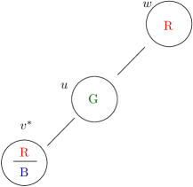
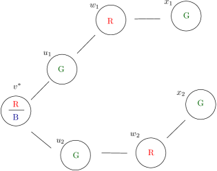
Figure 2: Left: the configuration $(3,2;(2),(1))$. Right: the configuration $(7,3;(3,3);(1,1))$.

In Chen et al. [5], to prove their improved result, they showed, via a linear program (LP), that although the $k>11/6$ result is tight for the flip probabilities $\{f_{i}\}$ in Vigoda’s original paper [37] (which are the same probabilities we used in Section 4), the analysis can be improved by weighting the single disagreement based on the configuration in the neighborhood of $v^{*}$. In particular, for each color $c$ which appears in the neighborhood of $v^{*}$, we consider the clusters involving $c$, namely the sets $\SS_{X_{t}}(c)$ and $\SS_{Y_{t}}(c)$. The only relevant information for these sets of clusters are the sizes of the clusters.

In Vigoda’s analysis there are six configurations of $\SS_{X_{t}}(c)$ and $\SS_{Y_{t}}(c)$ for which the analysis is tight; these are referred to as extremal configurations. By choosing slightly different flip probabilities, Chen et al. [5] reduce this to only two extremal configurations. Note that all non-extremal configurations have some slack in Vigoda’s analysis. Moreover, [5] showed that the extremal configurations are “brittle” and likely to flip to non-extremal configurations.

For pairs $(\sigma,\tau)\in\Omega^{2}$ which differ at a single vertex $v^{*}$, whereas their Hamming distance is one, [5] defined a new distance which is reduced by a factor $\eta$ for the fraction of colors that are in non-extremal configurations. [5] identified two specific configurations, up to symmetries: $(3,2;(2),(1))$ and $(7,3;(3,3),(1,1))$, which are the extremal configurations for their setting of flip probabilities.

Consider a pair $\sigma,\tau\in\Omega$ which differ at a single vertex $v^{*}$. We denote the colors with these extremal configurations on the neighborhood of $v^{*}$ as follows:

$$C^{1}(v^{*}) :=\{c:(A^{c},B^{c};a^{c},b^{c})\in\{(3,2;(2),(1)),(2,3;(1),(2))\}\}$$

$$C^{2}(v^{*}) :=\{c:(A^{c},B^{c};a^{c},b^{c})\in\{(7,3;(3,3),(1,1)),(3,7;(1,1),(3,3))\}\}.$$

Denote the fraction of neighbors of $v^{*}$ that are in extremal configurations as:

$$\gamma(v^{*})=\gamma_{\sigma,\tau}(v^{*}):=\left(|C^{1}(v^{*})|+2|C^{2}(v^{*})|\right)/\Delta.$$

Then, following [5], we can define the following distance between this pair of states $\sigma,\tau$ which differ at a single vertex $v^{*}$:

$$\mathcal{H}(\sigma,\tau):=1-\eta(1-\gamma_{\sigma,\tau}(v^{*}))$$

where $\delta=\frac{11}{6}-\frac{161}{88}=\frac{1}{264}$ and $1/2>\eta>0$ is a constant that we will define later.

Note that $\mathcal{H}(\sigma,\tau)$ is defined when $\sigma,\tau$ differ at a single vertex $v^{*}$, and this is extended to a metric on all of $\Omega^{2}$ using Definition B.1.

The advantage of this refined metric is that in the case of the extremal configurations, a single move of the flip dynamics is likely to change extremal to non-extremal configurations, which reduces the distance by a factor $\eta$ even though the Hamming distance stays the same. This yields some slack in the analysis of extremal configurations, which enables us to improve slightly on the 11/6 threshold, as is done in [5].

B.3 Contraction of the New Metric

We use the Path Coupling Theorem (Theorem B.2) to prove Theorem 1.2. To this end, we need to show that the new metric is contracting.

Chen et al. [5] showed that if we ignore the two extremal configurations then the maximum increase in Hamming distance per neighbor decreases from $\frac{11}{6}$ to $\frac{161}{88}=\frac{11}{6}-\frac{1}{264}$. This is obtained by solving an appropriate LP. Using this insight, we prove the following key result.

Lemma B.3.

There exists a constant $\varepsilon^{*}>0$ such that for all $k\geq(\frac{11}{6}-\varepsilon^{*})\Delta$ the following holds. Consider $X_{t},Y_{t}\in\Omega^{*}$ which differ at a single vertex, $v^{*}$. Then

$${\mathbf{E}\left({\mathcal{H}(X_{t+1},Y_{t+1})}\mid{X_{t},Y_{t}}\right)}\leq(1-\beta)\mathcal{H}(X_{t},Y_{t})$$

where $\beta>0$ is a small constant.

Theorem 1.2 follows immediately from Lemma B.3.

Proof of Theorem 1.2.

Combining Lemma B.3 with the path coupling Theorem B.2, we have

$$T_{\mathrm{mix}}\leq O\left(\frac{\log(|V|)}{\beta}\right)=O(\log{n}).$$

This completes the proof of Theorem 1.2. ∎

B.4 Contraction of the Hamming Metric

We first show a bound on the contraction of our original Hamming metric with our flip probabilities in the distributed setting. We prove the following analogue of Corollary 5.1 in [5], which bounds the expected change in Hamming distance from coupled flips.

One can check that when all neighbors of $v^{*}$ are extremal (i.e., $\gamma_{X_{t},Y_{t}}(v^{*})=1$), the change in $H$ is positive; when all neighbors are nonextremal, the change is negative. This agrees with the intuition that the “bad” configurations for Hamming distance are the extremal configurations.

In the following lemma, $\delta=\frac{11}{6}-\frac{161}{88}$ denotes the difference between the $\frac{11}{6}$ threshold in [37], and the lower ($\frac{11}{6}-\delta$) threshold that comes from considering only the non-extremal configurations as in [5]. The following lemma is the analog of Eq. 4 in the proof of Theorem 1.1; in short, Eq. 4 captures the expected change in Hamming distance by combining Lemma 4.8 (change from disagreement spreading) and Lemma 4.6 (disagreement disappearing).

Lemma B.4.

For the distributed flip dynamics, given $X_{t},Y_{t}$ differing at a single vertex $v^{*}$,

$$\sum_{c\in[k]}{\mathbf{E}\left({H(X_{t+1},Y_{t+1})\mathbf{1}(\mathcal{F}_{c})\mid X_{t},Y_{t}}\right)}\\ \leq(1-\alpha(1-\varepsilon^{*}/10^{7})\left(k-\left(\frac{11}{6}-\delta(1-\gamma(v^{*}))\right)\Delta\right)+\alpha\varepsilon^{*}\Delta/10^{7},$$ (11)

where $\mathcal{F}_{c}$ is defined in Lemma 4.8.

Proof.

Recall Eq. 4 in the proof of Theorem 1.1 where we proved the following for a color $c$ where $d_{c}(v^{*})\geq 1$:

$${\mathbf{E}\left({H(X_{t+1},Y_{t+1})\mathbf{1}(\mathcal{F}_{c})}\mid{X_{t},Y_{t}}\right)}\leq 1-\alpha(1-\varepsilon/5)\left[k-\frac{11}{6}d_{c}(v^{*})\right]+\alpha\varepsilon\Delta(28/30)$$ (4)

As mentioned earlier, whereas extremal configurations have expected change in Hamming distance $\leq\frac{11}{6}$, we can utilize [5, (22) in Observation 5.2] to obtain that the expected change in the Hamming distance is $\leq(\frac{11}{6}-\delta)$ for every non-extremal configuration. Since $(1-\gamma(v^{*}))\Delta$ of the neighbors of $v^{*}$ are non-extremal, combining the above with an easy analog of Lemma 4.6 yields the desired bound.

Recall we redefined $\alpha$ in this section so that $\alpha=\varepsilon^{*}/(10^{10}k)$ instead of $\varepsilon^{*}/(5000k)$. The term $\alpha\varepsilon\Delta(28/30)$ came from combining error terms obtained in Lemma 4.4, Lemma 4.6, and Lemma 4.8; retracing the proofs of those lemmas justifies our replacing this error term by $\alpha\varepsilon\Delta/10^{7}$ and similarly replacing $\varepsilon/5$ by $\varepsilon^{*}/10^{7}$. ∎

B.5 Decomposing the New Metric

To show that $\mathcal{H}$ is contracting, we want to show that the expected change in this metric is bounded. To this end, we decompose the expected change of $\mathcal{H}$ into two parts: the expected change in $H$ and the expected change from our new weighting colorings with extremal configurations. For ease of notation, let $\sigma=X_{t}$ and $\tau=Y_{t}$ denote the states at time $t$, and let $\sigma^{\prime}=X_{t+1}$ and $\tau^{\prime}=Y_{t+1}$ denote the (random) states at time $t+1$. We define

$$B(\sigma,\tau):=H(\sigma,\tau)-\mathcal{H}(\sigma,\tau)$$ (12)

to denote the difference from Hamming distance, and note that $B$ is not a metric. Observe that $\mathcal{H}$ increases when either $H$ increases or $B$ decreases. Thus the idea now is to use the slack given by the non-extremal configurations (in Lemma B.4) to show that the expected increase in the Hamming metric $H(\sigma,\tau)$—whenever this increase is positive—is offset by the (sufficiently large) expected increase in $B$, giving a net decrease in the metric $\mathcal{H}$. We do so by bounding the following division of the expected change:

$$\nabla_{\mathcal{H}}=\nabla_{\mathcal{H}}(\sigma,\tau) :={\mathbf{E}\left({\mathcal{H}(\sigma^{\prime},\tau^{\prime})-\mathcal{H}(\sigma,\tau)}\right)},$$

$$\nabla_{H}=\nabla_{H}(\sigma,\tau) :={\mathbf{E}\left({H(\sigma^{\prime},\tau^{\prime})-H(\sigma,\tau)}\right)}={\mathbf{E}\left({H(\sigma^{\prime},\tau^{\prime})-1}\right)}\text{, and}$$

$$\nabla_{B}=\nabla_{B}(\sigma,\tau) :={\mathbf{E}\left({B(\sigma^{\prime},\tau^{\prime})-B(\sigma,\tau))}\right)},$$

Note that $\nabla_{H}$ is simply equal to the change in Hamming distance, and hence  Lemma B.4 bounds $\nabla_{H}$. Furthermore $\nabla_{\mathcal{H}}=\nabla_{H}-\nabla_{B}$. Thus our aim is to bound $\nabla_{H}$ from above and bound $\nabla_{B}$ from below.

Lemma B.4 bounds the contribution to $\nabla_{\mathcal{H}}$ from the event $\mathcal{F}_{c}$ (recall that this is the event that one of the non-identity-coupled flips of distance-1 flips occurs). Bounding the contribution from distance-2 flips is the same as in Lemma 4.4, and bounding the contribution from distance-0 flips is the same as in Lemma 4.6.

Let $C^{0}(v^{*})=[k]\setminus(C^{1}(v^{*})\cup C^{2}(v^{*}))$ denote the set of colors that do not appear in an extremal configuration with respect to $v^{*}$. For a color $c\in[k]$ and for all $i,j\in\{0,1,2\}$, let $\mathcal{E}_{i,j}(c)$ denote the event that $c\in C^{i}_{X_{t},Y_{t}}(v^{*})$ and $c\in C^{j}_{X_{t+1},Y_{t+1}}(v^{*})$, i.e., at time $t$ color $c$ is in $C^{i}(v^{*})$ and then after the coupled update color $c$ is in $C^{j}(v^{*})$. Moreover, let

$$E_{i,j}(c)={\mathbf{E}\left({\mathbf{1}(\mathcal{E}_{i,j}(c)}\right)}.$$

Then it follows that

$$\nabla_{B}\geq\frac{\eta}{\Delta}\sum_{c\in C^{1}(v^{*})\cup C^{2}(v^{*})}\left[E_{1,0}(c)+2E_{2,0}(c)-E_{1,2}(c)\right]\hskip 14.45377pt-\frac{\eta}{\Delta}\sum_{c\in C^{0}(v^{*})}\left[E_{0,1}(c)+2E_{0,2}(c)\right].$$ (13)

(We ignore $E_{2,1}(c)$ since including it would only make the bound better.)

The following lemmas are the analog of [5, Lemma 5.2]; we both simplify their case analysis and handle some subtleties that arise from the distributed setting.

Lemma B.5.

$$\sum_{c\in C^{1}(v^{*})\cup C^{2}(v^{*})}\left[E_{1,0}(c)+2E_{2,0}(c)\right]\geq\alpha(1-\varepsilon_{1})\left(k-\Delta-2\right)\gamma(v^{*})$$

where $\varepsilon_{1}=1-(1-\varepsilon^{*}/250)^{2}(1-4\alpha k)$.

Lemma B.6.

$$\sum_{c\in C^{0}(v^{*})}\left[E_{0,1}(c)+2E_{0,2}(c)+E_{1,2}(c)\right]\leq(52\alpha k)(1-\gamma(v^{*}))+(\alpha\Delta/2)\gamma(v^{*})$$

Proof of Lemma B.5.

Let $c\in C^{1}(v^{*})\cup C^{2}(v^{*})$ and let $R=X_{t}(v^{*})$ and $B=Y_{t}(v^{*})$. Then there exists $u\in N(v^{*})$ and $w\in N(u)$ such that $X_{t}(u)=Y_{t}(u)=c$ and $X_{t}(w)=Y_{t}(w)\in\{R,B\}$. It follows that if $w$ flips to a color not in $\{R,B\}$ and no other flip changes the color of $v^{*}$, the color of a neighbor of $v^{*}$ does not flip to $c$, and the color of a neighbor of $u$, then $u\not\in C^{1}(v^{*})\cup C^{2}(v^{*})$ at time $t+1$. We will now show a lower bound on the probability of this event occurring.

There are at least $k-\Delta-2$ colors not in the neighborhood of $w$ that are not in $\{R,B\}$. For each of these colors $c^{\prime}$, the probability of flipping the singleton cluster $S=S_{\sigma}(w,c^{\prime})=S_{\tau}(w,c^{\prime})$ is $\geq\alpha(1-\varepsilon^{*}/250)^{2}$ by Lemma 5.1 (recall $\varepsilon^{*}$ in this section replaces $\varepsilon$ from Sections 4.2 and 5).

There are at most $\Delta-1$ neighbors of $v^{*}$ that could flip to color $c$. Hence, there are at most $\Delta\leq k$ clusters that if flipped would change the a neighbor of $v^{*}$ to color $c$. There are at most $k$ clusters that contain $v^{*}$. Finally, there are at most $2\Delta$ clusters that if flipped would flip a neighbor of $u$ to a color in $\{R,B\}$. The probability of any of these clusters flipping is at most $\alpha f_{1}$. Hence, the probability of none of these clusters flipping is at least $(1-4k\alpha)$.

Thus, for $c\in C^{i}(v^{*})$ for $i\in\{1,2\},$

$$E_{i,0}(c)\geq\alpha(1-\varepsilon_{1})(1-4\alpha k)(k-\Delta-2).$$ (14)

We note that this bound is not very tight. Namely if $c\in C^{2}(v^{*})$ then we could find at least one more vertex $y$ such that $X_{t}(y)=Y_{t}(y)\in\{R,B\}$ and flipping it to a color not in $\{R,B\}$ (and assuming no other clusters flip near it) would result in $c\not\in C^{1}(v^{*})\cup C^{2}(v^{*})$ for step $t+1$. However, this is not necessary for our final analysis. ∎

Proof of Lemma B.6.

Fix a color $c$. Denote $X_{t}(v^{*})$ as $R$, $Y_{t}(v^{*})$ as $B$ and $c$ as $G$.

We begin by upper bounding $E_{0,1}(c)$. Suppose $c\in C^{0}(v^{*})$ at step $t$ but $c\in C^{1}(v^{*})$ at step $t+1$. and let $u\in N(v^{*})$ denote the unique $G$ neighbor of $v^{*}$ at time $t+1$. If this occurs it must be the case that one of the following events occurred:

1. Suppose that $u$ was not $G$ at time $t$. Then a neighbor of $v^{*}$ flipped to color $G$ at time $t+1$. There are at most $\Delta$ clusters that if flipped would result in a neighbor of $v^{*}$ flipping to $G$ from a different color.

2. Suppose $u$ was $G$ at time $t$ and $d_{G}(v^{*})\geq 2$. In this case, at least $d_{G}(v^{*})-1$ neighbors of $v^{*}$ flipped from $G$ to a different color at time $t+1$. Consider any two distinct $u_{1},u_{2}\in N(v^{*})$ where $u_{1}$ and $u_{2}$ are $G$ in both chains at time $t$. At least one of these neighbors flipped from color $G$ to a different color, and there are at most $2k$ clusters that if flipped would result in $u_{1}$ or $u_{2}$ changing color.

3. If neither (1) or (2) occur, it must be the case that $d_{G}(v^{*})=1$. Let $d$ denote the number of neighbors of $u$ (excluding $v^{*}$) that are $R$ or $B$ at time $t$ and let $w\in N(u)\setminus\{v^{*}\}$ unique neighbor of $u$ that is $R$ or $B$ at time $t+1$

   1. Suppose that $w$ was not $R$ or $B$ at time $t$. Then a neighbor of $u$ flipped to $G$ at time $t+1$. There are at most $\Delta$ clusters that if flipped would result in a neighbor of $u$ flipping to $G$ from a different color.

   2. Suppose $w$ was $R$ or $B$ at time $t$ and $d\geq 2$. Then, at least $d-1$ vertices flip from $R$ or $B$ to a color not in $\{R,B\}$. Similar to before, it follows that $d_{R}(v^{*})+d_{B}(v^{*})\geq 2$, then consider $w_{1}$ and $w_{2}$ that are $R$ or $B$ in both chains at step $t$. At least one of $w_{1}$ and $w_{2}$ flipped to a color not in $\{R,B\}$. There are at most $2k$ clusters that if flipped would have resulted in $w_{1}$ or $w_{2}$ flipping from to a color not in $\{R,B\}$.

   3. If neither (a) or (b) occur then it follows that $d=1$. Since $G$ is non-extremal there exists at least one $z\in N(w)\setminus\{u\}$ which is colored $G$ at time $t$. The vertex $z$ must have been recolored to a non-$G$ color at time $t+1$. There are at most $k$ clusters that if flipped will recolor $z$.

We note that depending on the initial state of the chains several of the above cases are feasible to occur, for example, (1) and (3) can both be possible or (3a) and (3c) can both be possible. For this reason, we get a weak but sufficient upper bound by union bounding over the above events. Therefore, $E_{0,1}(c)\leq\alpha(\Delta+2k+2\Delta+2k+k)\leq 8\alpha k$.

An analogous case analysis shows that $2E_{0,2}(c)\leq 44\alpha k$. To bound $E_{0,2}(c)$ in this way we also have to allow for more than one vertex in a neighbor to be a color in $\{R,G,B\}$. Namely, for $E_{0,2}(c)$ to occur, there must be exactly two neighbors $u_{1}$ and $u_{2}$ of $v^{*}$ that are color $G$ at step $t+1$. This means that we need to change case (2) to be the case that $d_{G}(v^{*})\geq 3$ at step $t$. Likewise, in case (3), we now have $d_{G}(v^{*})=2$. We will then have cases analogous to cases (3a), (3b) and (3c) for $u_{1}$ and $u_{2}$. At step $t+1$ there are two cases for $u\in\{u_{1},u_{2}\}$:

1. The vertex $u$ has exactly two neighbors $w_{1},w_{2}$ that are both of color $R$ or both of color $B$ and ${w_{1},w_{2}}$ has no neighbor besides $u$ of color $G$.

2. The vertex $u$ has a unique neighbor $w$ of color $R$ or $B$, $w$ has exactly one other neighbor $z$ of color $G$, and $z$ has no other neighbor besides $w$ of color $R$ or $B$.

Finally, we note that the coefficient $44$ is far from optimal but is sufficient for our analysis.

Finally, if $c\in C^{1}(v^{*})$ at step $t$ and $c\in C^{2}(v^{*})$ at step $t+1$. Then there exists a unique $u\in N(v^{*})$ and $w\in N(u)\setminus\{v^{*}\}$ such that $u$ is color $G$, $w$ is color $R$ or color $B$ and no neighbor of $w$ besides $u$ is color $G$. For the event to occur, it must be the case that a neighbor of $v^{*}$ besides $u$ and a neighbor of $w$ besides $u$ must flip to color $G$. Note, these can not be the same vertices if $c\in C^{2}(v^{*})$ at step $t+1$. Thus, either a cluster of size at least $2$ has to flip with probability $\alpha f_{2}$ or two clusters of size at least one have to flip with probability $\alpha^{2}$. In either case, $E_{1,2}(c)\leq\frac{1}{2}\alpha k$.

∎

B.6 Combining $\nabla_{H},\nabla_{B}$ to Prove Lemma B.3

Proof of Lemma B.3.

Recall, our goal is to show that there exists $\beta>0$ such that

$${\mathbf{E}\left({\mathcal{H}(X_{t+1},Y_{t+1})}\mid{X_{t},Y_{t}}\right)}\leq(1-\beta)\mathcal{H}(X_{t},Y_{t}).$$

First we bound $\nabla_{B}$ by combining Lemma B.5 and Lemma B.6.

Recall that we have deferred defining $\eta$ until now. Recall $\delta=\frac{11}{6}-\frac{161}{88}=\frac{1}{264}$. We now define

$$\eta=\left((1-\varepsilon_{1})\left(1-\frac{8}{5}\left(\frac{11}{6}-\varepsilon^{*}\right)^{-1}\right)+52\right)^{-1}\frac{\delta\Delta}{k}.$$

Notice that $0<\eta<1$. The term $\frac{\delta\Delta}{k}$ allows us to obtain useful cancellations. satisfy $0<\rho<1$, as we need a convex combination of $\gamma(v^{*})$ and $1-\gamma(v^{*})$ to make the subsequent inequalities work.

For convenience we will name the constant term in $\eta$: let

$$\psi=\left((1-\varepsilon_{1})\left(1-\frac{8}{5}\left(\frac{11}{6}-\varepsilon^{*}\right)^{-1}\right)+52\right)^{-1}$$

and $\eta=\psi\frac{\delta\Delta}{k}$. Define $\rho=52\psi$. We have chosen $\psi$ and $\rho$ so that $0<\rho<1$; this will enable us to obtain a convex combination $(1-\rho)\gamma(v^{*})-\rho(1-\gamma(v^{*}))$ in the following inequalities. We get the following inequality:

$$\nabla_{B} \geq\frac{\eta}{\Delta}\sum_{c\in C^{1}(v^{*})\cup C^{2}(v^{*})}\left[E_{1,0}(c)+2E_{2,0}(c)-E_{1,2}(c)\right]-\frac{\eta}{\Delta}\sum_{c\in C^{0}(v^{*})}\left[E_{0,1}(c)+2E_{0,2}(c)\right]$$

$$\geq\alpha\eta(1-\varepsilon_{1})\left(\frac{k}{\Delta}-\frac{3}{2}-\frac{2}{\Delta}\right)\gamma(v^{*})\Delta-52\alpha\eta\frac{k}{\Delta}(1-\gamma(v^{*}))\Delta-\alpha\Delta\varepsilon^{*}/10^{7}$$

$$=\alpha\delta\psi\left((1-\varepsilon_{1})\left(1-\frac{3\Delta}{2k}-\frac{2}{k}\right)\gamma(v^{*})-52(1-\gamma(v^{*}))\right)\Delta-\alpha\Delta\varepsilon^{*}/10^{7}$$

$$\geq\alpha\delta\psi\left((1-\varepsilon_{1})\left(1-\frac{8}{5}\cdot\left(\frac{11}{6}-\varepsilon^{*}\right)^{-1}\right)\gamma(v^{*})-52(1-\gamma(v^{*})\right)\Delta-\alpha\Delta\varepsilon^{*}/10^{7}$$

$$\geq\alpha\delta\left((1-\rho)\gamma(v^{*})-\rho(1-\gamma(v^{*}))\right)\Delta-\alpha\Delta\varepsilon^{*}/10^{7},$$ (15)

where in the second line we have applied Lemma B.5 and Lemma B.6, and in the third line we have applied the substitution $\eta=\psi\frac{\Delta}{k}$. In the fourth line we have used the fact that $k\geq\left(\frac{11}{6}-\varepsilon^{*}\right)\Delta$ so that $\frac{3\Delta}{2k}+\frac{2}{k}\leq\frac{8}{5}\left(\frac{11}{6}-\varepsilon^{*}\right)^{-1}$ for $\varepsilon^{*}$ sufficiently small.

Combining Lemma B.4 and Eq. 15 we get

$${\mathbf{E}\left({\mathcal{H}(X_{t+1},Y_{t+1}))}\mid{X_{t}=\sigma,Y_{t}=\tau}\right)}-\mathcal{H}(\sigma,\tau)$$

$$\qquad\leq\nabla_{H}-\nabla_{B}$$

$$\qquad\leq\alpha(1-\varepsilon^{*}/10^{7})\left(\left(\frac{11}{6}-\delta(1-\gamma_{\sigma,\tau}(v^{*}))\right)\Delta-k\right)\ +\alpha\Delta\varepsilon^{*}/10^{7}+\alpha\Delta\varepsilon^{*}/10^{7}$$

$$\qquad\qquad+\alpha\delta\left(\rho(1-\gamma_{\sigma,\tau}(v^{*}))-(1-\rho)\gamma(v^{*})\right)\Delta$$

$$\qquad\leq\alpha(1-\varepsilon^{*}/10^{7})\left(\left(\frac{11}{6}-\delta(1-\rho)\right)\Delta-k\right)+\alpha\Delta\varepsilon^{*}/10^{6}$$

$$\qquad\leq-\alpha\mu k+\alpha\Delta\varepsilon^{*}/10^{6},$$

where

$$\mu=(1-\varepsilon^{*}/10^{7})\left(1-\left(\frac{11}{6}-\delta(1-\rho)\right)\frac{\Delta}{k}\right)\geq(1-\varepsilon^{*}/10^{7})\left(1-\left(\frac{11}{6}-\delta(1-\rho)\right)\left(\frac{11}{6}-\varepsilon^{*}\right)^{-1}\right)>0,$$

since $\varepsilon^{*}<\delta(1-\rho)$ for sufficiently small $\varepsilon^{*}$.

Let $\beta=\alpha\mu k-\alpha\Delta\varepsilon^{*}/10^{6}$. We now show that $\beta>0$:

$$\beta =\alpha\mu k-\alpha\Delta\varepsilon^{*}/10^{6}$$

$$=(\varepsilon^{*}/10^{10})(\mu-(\Delta/k)/10^{6})$$

$$\geq(\varepsilon^{*}/10^{10})\left(\mu-\left(\frac{11}{6}-\varepsilon^{*}\right)^{-1}(1/10^{6})\right)$$

$$\geq(\varepsilon^{*}/10^{10})\left(1-\left(\frac{1}{10^{6}(1-\varepsilon^{*}/10^{7})}+\frac{11}{6}-\delta(1-\rho)\right)\left(\frac{11}{6}-\varepsilon^{*}\right)^{-1}\right)$$

$$>0,$$

where in the second line we have applied the definition of $\alpha$, and in the fourth line we have applied the definition of $\mu$. The fifth line follows from the fact that:

$$\delta(1-\rho)=\left(\frac{11}{6}-\frac{161}{88}\right)(1-\rho)>10^{6}(1-\varepsilon^{*}/10^{7}).$$

Finally, since $\mathcal{H}(\sigma,\tau)\leq 1$, rearranging we get

$${\mathbf{E}\left({\mathcal{H}(X_{t+1},Y_{t+1}))}\mid{X_{t}=\sigma,Y_{t}=\tau}\right)}\leq(1-\beta)\mathcal{H}(\sigma,\tau).$$

∎

References

- [1] Leonid Barenboim, Michael Elkin, and Uri Goldenberg. Locally-iterative distributed -coloring and applications. Journal of the ACM, 69(1):Article 5, 2021.
- [2] Leonid Barenboim, Michael Elkin, Seth Pettie, and Johannes Schneider. The locality of distributed symmetry breaking. Journal of the ACM, 63(3), 2016.
- [3] Anton Bernshteyn, Tyler Brazelton, Ruijia Cao, and Akum Kang. Counting colorings of triangle-free graphs. Journal of Combinatorial Theory, Series B, 161:86–108, 2023.
- [4] Russ Bubley and Martin E. Dyer. Path coupling: a technique for proving rapid mixing in Markov chains. In Proceedings of the 38th Annual IEEE Symposium on Foundations of Computer Science (FOCS), pages 223–231, 1997.
- [5] Sitan Chen, Michelle Delcourt, Ankur Moitra, Guillem Perarnau, and Luke Postle. Improved bounds for randomly sampling colorings via linear programming. In Proceedings of the 30th Annual ACM-SIAM Symposium on Discrete Algorithms (SODA), pages 2216–2234, 2019.
- [6] Zongchen Chen, Kuikui Liu, Nitya Mani, and Ankur Moitra. Strong spatial mixing for colorings on trees and its algorithmic applications. In Proceedings of the 64th IEEE Symposium on Foundations of Computer Science (FOCS), 2023.
- [7] Constantinos Daskalakis, Nishanth Dikkala, and Siddhartha Jayanti. Hogwild!-Gibbs can be panaccurate. In Proceedings of the 31st Advances in Neural Information Processing Systems (NeurIPS), page 32–41, 2018.
- [8] Christopher De Sa, Kunle Olukotun, and Christopher Ré. Ensuring rapid mixing and low bias for asynchronous Gibbs sampling. In Proceedings of the 33rd International Conference on Machine Learning (ICML), page 1567–1576, 2016.
- [9] Martin Dyer, Alan Frieze, Thomas P. Hayes, and Eric Vigoda. Randomly coloring constant degree graphs. Random Structures & Algorithms, 43(2):181–200, 2013.
- [10] Martin Dyer and Catherine Greenhill. Random walks on combinatorial objects. Surveys in Combinatorics, page 101–136, 1999.
- [11] Weiming Feng, Thomas P. Hayes, and Yitong Yin. Distributed symmetry breaking in sampling (optimal distributed randomly coloring with fewer colors). arXiv preprint arXiv:1802.06953, 2018.
- [12] Weiming Feng, Yuxin Sun, and Yitong Yin. What can be sampled locally? In Proceedings of the International Symposium on Principles of Distributed Computing (PODC), page 121–130, 2017.
- [13] Weiming Feng and Yitong Yin. On local distributed sampling and counting. In Proceedings of the 37th ACM Symposium on Principles of Distributed Computing (PODC), pages 189–198, 2018.
- [14] Manuela Fischer and Mohsen Ghaffari. A simple parallel and distributed sampling technique: Local Glauber dynamics. In 32nd International Symposium on Distributed Computing (DISC), volume 121, pages 26:1–26:11, 2018.
- [15] Xinyu Fu, Yitong Yin, and Chaodong Zheng. Locally-iterative -coloring in sublinear (in ) rounds. arXiv preprint arXiv:2207.14458, 2023.
- [16] Marc Fuchs and Fabian Kuhn. Brief announcement: List defective colorings: Distributed algorithms and applications. In Proceedings of the 35th ACM Symposium on Parallelism in Algorithms and Architectures (SPAA), 2023.
- [17] Joseph Gonzales, Yucheng Low, Arthur Gretton, and Carlos Guestrin. Parallel Gibbs sampling: From colored fields to thin junction trees. In Proceedings of the 14th International Conference on Artificial Intelligence and Statistics (AISTATS), volume 15, pages 324–332, 2011.
- [18] G.E. Hinton. Training products of experts by minimizing contrastive divergence. Neural computation, 14(8):1771–1800, 2002.
- [19] G.E. Hinton, S. Osindero, and Y-W. Teh. A fast learning algorithm for deep belief nets. Neural computation, 18(7):1527–1554, 2006.
- [20] G.E. Hinton and R.R. Salakhutdinov. Replicated softmax: an undirected topic model. In Advances in Neural Information Processing Systems (NeurIPS), pages 1607–1614, 2009.
- [21] Mark Jerrum. A very simple algorithm for estimating the number of -colorings of a low-degree graph. Random Structures & Algorithms, 7(2):157–165, 1995.
- [22] Michael I. Jordan, Jason D. Lee, and Yun Yang. Communication-efficient distributed statistical inference. Journal of the American Statistical Association, 2018.
- [23] Christos Karras, Aristeidis Karras, Dimitrios Tsolis, Konstantinos C. Giotopoulos, and Spyros Sioutas. Distributed gibbs sampling and lda modelling for large scale big data management on pyspark. In 2022 7th South-East Europe Design Automation, Computer Engineering, Computer Networks and Social Media Conference (SEEDA-CECNSM), pages 1–8, 2022.
- [24] Daphne Koller and Nir Friedman. Probabilistic Graphical Models: Principles and Techniques. MIT Press, 2009.
- [25] Fabian Kuhn. Weak graph colorings: Distributed algorithms and applications. In Proceedings of the 21st ACM Symposium on Parallelism in Algorithms and Architectures (SPAA), pages 138–144, 2009.
- [26] Nathan Linial. Locality in distributed graph algorithms. SIAM Journal on Computing, 21(1):193–201, 1992.
- [27] Hongyang Liu and Yitong Yin. Simple parallel algorithms for single-site dynamics. In 54th Annual ACM SIGACT Symposium on Theory of Computing (STOC), pages 1431–1444, 2022.
- [28] Kevin P. Murphy. Machine learning: a probabilistic perspective. MIT Press, 2012.
- [29] Moni Naor and Larry Stockmeyer. What can be computed locally? In Proceedings of the 25th Annual ACM Symposium on Theory of Computing (STOC), pages 184–193, 1993.
- [30] S. Osindero and G.E. Hinton. Modeling image patches with a directed hierarchy of Markov random fields. In Advances in Neural Information Processing Systems (NeurIPS), pages 1121–1128, 2008.
- [31] R. Salakhutdinov and G.E. Hinton. Deep Boltzmann machines. In Proceedings of the 12th International Conference on Artificial Intelligence and Statistics (AISTATS), pages 448–455, 2009.
- [32] R. Salakhutdinov, A. Mnih, and G.E. Hinton. Restricted Boltzmann machines for collaborative filtering. In Proceedings of the 24th International Conference on Machine Learning (ICML), pages 791–798, 2007.
- [33] Jesús Salas and Alan D. Sokal. Absence of phase transition for antiferromagnetic Potts models via the Dobrushin uniqueness theorem. Journal of Statistical Physics, 86(3-4):551–579, 1997.
- [34] Johannes Schneider and Roger Wattenhofer. A new technique for distributed symmetry breaking. In Proceedings of the 29th ACM SIGACT-SIGOPS Symposium on Principles of Distributed Computing (PODC), page 257–266, 2010.
- [35] Alexander Smola and Shravan Narayanamurthy. An architecture for parallel topic models. In Proceedings of the VLDB Endowment (PVLDB), 2010.
- [36] Alexander Terenin, Daniel Simpson, and David Draper. Asynchronous Gibbs sampling. In Proceedings of the 23rd International Conference on Artificial Intelligence and Statistics (AISTATS), page 144–154, 2020.
- [37] Eric Vigoda. Improved bounds for sampling colorings. Journal of Mathematical Physics, 41(3):1555–1569, 2000.
- [38] Feng Yan, Ningyi Xu, and Yuan Qi. Parallel inference for latent dirichlet allocation on graphics processing units. In Advances in Neural Information Processing Systems (NeurIPS), volume 22, 2009.
- [39] Yuan Yang, Jianfei Chen, and Jun Zhu. Distributing the stochastic gradient sampler for large-scale LDA. In Proceedings of the 22nd ACM SIGKDD International Conference on Knowledge Discovery and Data Mining (KDD), page 1975–1984, 2016.
- [40] Ce Zhang and Christopher Ré. Dimmwitted: A study of main-memory statistical analytics. In Proceedings of the VLDB Endowment (PVLDB), 2014.