Large $N$ Universality of 4d $\mathcal{N}=1$ Superconformal Index and AdS Black Holes

Abstract

We study the large $N$ limit of the matrix models associated with the superconformal indices of four-dimensional $\mathcal{N}=1$ superconformal field theories. We find that for a large class of $\mathcal{N}=1$ superconformal gauge theories, the superconformal indices in the large $N$ limit of such theories are dominated by the ‘parallelogram’ saddle, providing $O(N^{2})$ free energy for the generic value of chemical potentials. This saddle corresponds to BPS black holes in AdS₅ whenever a holographic dual description is available. Our saddle applies to a large class of gauge theories, including ADE quiver gauge theories, and the theories with rank-2 tensor matters. Our analysis works for most $\mathcal{N}=1$ superconformal gauge theories that admit a suitable large $N$ limit while keeping the flavor symmetry fixed. We also find ‘multi-cut’ saddle points, which correspond to the orbifolded Euclidean black holes in AdS₅.

1 Introduction

One of the crucial implications of the AdS/CFT correspondence Maldacena:1997re ; Gubser:1998bc ; Witten:1998qj is that the boundary conformal field theories (CFTs) should exhibit a universal thermodynamic phase, in which the bulk black hole geometry emerges. This universal property of (holographic) CFTs is independent of the details of the theory Hawking:1982dh ; Witten:1998zw . One ideal setting to study such a phenomenon is to focus on the BPS sector, which has been an extremely useful setting, as was demonstrated in the microscopic derivation of the Bekenstein-Hawking entropy by Strominger-Vafa Strominger:1996sh . We would like to take a similar strategy to understand bulk geometry from the BPS sector of the boundary. In the BPS sector, one can exactly compute the BPS observables of superconformal field theories (SCFTs); hence, quantitative analysis can be carried out.

Relatedly, another pressing question in AdS/CFT is to find a precise condition for the CFT in which the holographic bulk description in terms of a weakly-coupled Einstein gravity emerges. For the case of two-dimensional CFTs, such conditions have been discussed in Hartman:2014oaa utilizing the modular invariance of the thermal partition function. Assuming the existence of Hawking-Page-like phase transition between the graviton gas phase and the large AdS black hole phase, the authors of Hartman:2014oaa were able to derive the Bekenstein-Hawking entropy formula, which has the same form as the Cardy formula. However, the crucial difference here is that the Cardy formula has a very different regime of validity (finite central charge, very large scaling dimension $\Delta\gg c$) from the large AdS black hole (large central charge $c\gg 1$, scaling dimension of order $\Delta>c/12$). A similar analysis was also carried out for SCFTs in 2d using the elliptic genus Benjamin:2015hsa ; Benjamin:2015vkc .

We would like to tackle similar questions in the AdS₅/CFT₄ context. Which 4d SCFTs are holographically dual to a weakly-coupled Einstein gravity? When do we have emergent black hole geometry? More modestly, we aim to find SCFTs with a phase potentially described by the large BPS black holes in AdS. To this end, we shall study the large $N$ behavior of the superconformal index Romelsberger:2005eg ; Kinney:2005ej for the 4d $\mathcal{N}=1$ SCFTs, which are realized from (the IR fixed point of) $\mathcal{N}=1$ supersymmetric gauge theories. The superconformal index enumerates the $(-1)^{F}$-graded degeneracy of certain BPS states in the radially quantized SCFT on $S^{3}$. One of the original motivations of the index is to account for the Bekenstein-Hawking entropy of the BPS black holes in AdS₅ Gutowski:2004ez ; Gutowski:2004yv ; Chong:2005hr ; Kunduri:2006ek . This goal was realized a decade later by a series of works utilizing the complex saddles of the large $N$ index from various viewpoints starting from Cabo-Bizet:2018ehj ; Choi:2018hmj ; Benini:2018ywd . Subsequently, various developments have been made using different methods, such as Cardy-like limits (also in finite $N$) Choi:2018hmj ; Choi:2018vbz ; Honda:2019cio ; ArabiArdehali:2019tdm ; Kim:2019yrz ; Cabo-Bizet:2019osg ; Amariti:2019mgp ; Goldstein:2020yvj ; Jejjala:2021hlt , and Bethe-Ansatz type formula Closset:2017bse ; Benini:2018mlo for the large $N$ index Benini:2018ywd ; Lanir:2019abx ; GonzalezLezcano:2019nca ; Benini:2020gjh and particular extension of the index integral Cabo-Bizet:2019eaf ; Cabo-Bizet:2020nkr .

The main result of this paper is to show that the matrix model of the index for this large class of gauge theories admits a universal large $N$ saddle point, called the ‘parallelogram ansatz,’ which accounts for the $O(N^{2})$ free energy necessary to account for the black holes. It was first discovered for the $\mathcal{N}=4$ $U(N)$ supersymmetric Yang-Mills theory (SYM) in Choi:2021rxi that works beyond the particular limit (such as one parameter or certain ratio) of the fugacities in the previous studies, and also showed that it is indeed a genuine saddle point of the index integral, without any ad hoc assumption. This large $N$ solution is independent of the details of the theory and only depends on the angular momentum fugacities on $S^{3}$, thus being universal. We demonstrate how it can be generalized to $\mathcal{N}=1$ gauge theories, which allows generic holographic theories to account for the universal BPS black holes in AdS₅ Gutowski:2004ez ; Gutowski:2004yv ; Chong:2005hr ; Kunduri:2006ek .

We find that such saddle point exists for a large class of gauge theories admitting a suitable large $N$ limit. In particular, it works for a gauge theory with a finite number of matter fields in arbitrary rank-one or rank-two representations under the gauge group. It works for all simple large $N$ gauge theories with a fixed flavor symmetry, which is classified in Agarwal:2020pol . The saddle also works for the quiver gauge theories with $SU(N)$, $SO(N)$, and $Sp(N)$ gauge nodes. The prime examples are the Klebanov-Witten theory Klebanov:1998hh , toric models such as the $Y^{p,q}$-theories Martelli:2004wu ; Benvenuti:2004dy , and, of course, the $\mathcal{N}=4$ super-Yang-Mills theories with $SU(N)$, $SO(N)$, or $Sp(N)$ gauge group. The ‘parallelogram saddle’ works for most of the known holographic Lagrangian gauge theories, and accounts for the $O(N^{2})$ free energy of the AdS black holes. The list of theories that do not admit our saddle point includes supersymmetric quantum chromodynamics (SQCD) in the conformal window, class $\mathcal{S}$ theories with full punctures Gaiotto:2009we , and the theories with a ‘dense spectrum’ Agarwal:2019crm ; Agarwal:2020pol . This does not rule out the possibility of another kind of saddle responsible for the black hole phase.

The superconformal index we study is defined as Kim:2019yrz ; Cabo-Bizet:2020nkr ; Cassani:2021fyv

$$\mathcal{I}(\sigma,\tau)=\Tr\left[e^{-\pi iR}e^{2\pi i\sigma\left(J_{1}+\frac{R}{2}\right)}e^{2\pi i\tau\left(J_{2}+\frac{R}{2}\right)}\right]\ ,$$ (1)

where the trace is taken over the Hilbert space of radially quantized SCFT on $S^{3}$. Here, $J_{1}$, $J_{2}$ are the Cartan charges of $SO(4)$ rotation symmetry, and $R$ is the superconformal $U(1)_{R}$ $R$-charge. We can also include the fugacities for the flavor symmetries. Notice that we have inserted $e^{-\pi iR}$ instead of the usual $(-1)^{F}$. This version of the index turns out to exhibit a deconfinement phase in the Cardy-like limit $\sigma,\tau\to 0$, whereas the old version does not Kim:2019yrz ; Cabo-Bizet:2019osg . The former is related to the latter by going to the ‘second sheet’ in the chemical potential space Cassani:2021fyv . It was shown that in the Cardy-like limit $\sigma,\tau\to 0$, the index takes the universal expression Choi:2018hmj ; Kim:2019yrz ; Cabo-Bizet:2019osg

$$\log\mathcal{I}(\sigma,\tau)\sim-\,(5a-3c)\;\frac{2i\pi\delta^{3}}{27\sigma\tau}-(a-c)\frac{4\pi i\delta}{3\sigma\tau}\ ,$$ (2)

which is completely determined by the central charges $a$ and $c$. Here, $\delta\equiv\frac{\sigma+\tau-1}{2}$. This expression holds without taking any large $N$ limit, which serves as an analog of Cardy’s formula in two-dimensions Cardy:1986ie . The Cardy-like formula reproduces the Bekenstein-Hawking entropy of large BPS black holes in AdS₅ Gutowski:2004ez ; Gutowski:2004yv ; Chong:2005hr ; Kunduri:2006ek whenever the holographic dual of SCFT is known. However, we know that the black hole threshold ($\Delta\sim c$) is much lower than that of the Cardy limit ($\Delta\gg c$). Therefore, this formula does not a priori apply to the black holes near the threshold.

In this paper, using the parallelogram ansatz for the index matrix model, we obtain a universal large $N$ formula for the index of 4d $\mathcal{N}=1$ SCFTs, which is given by

$$\log\mathcal{I}(\sigma,\tau)\sim-\,(5a-3c)\;\frac{2i\pi\delta^{3}}{27\sigma\tau}\ ,$$ (3)

with $\delta=\frac{\sigma+\tau-1}{2}$. Here, $a\sim c=O(N^{2})$, and we only kept the terms of order $O(N^{2})$, where $N$ is the rank of the gauge group. Notice that this formula agrees with the Cardy-like formula (2) without taking the Cardy limit. This expression gives the dominant contribution for the free-energy above the black hole threshold, which is far below the Cardy limit. For holographic theories, the above formula perfectly captures the Bekenstein-Hawking entropy of the universal BPS black holes in AdS₅. If we turn on the flavor chemical potentials, the above formula is generalized as

$$\log\mathcal{I}(\Delta,\sigma,\tau)\sim-\,\frac{i\pi}{24\sigma\tau}\sum_{I,J,K}\Tr(Q^{I}Q^{J}Q^{K})\,\Delta_{I}\Delta_{J}\Delta_{K}\ ,$$ (4)

where $2Q^{I}$’s are various candidate $R$-charges made by the linear combinations of true superconformal $R$-charge and flavor charges, and $\Delta_{I}$’s are the corresponding chemical potentials. (For a precise definition, see Section 2.) One can see that the ’t Hooft anomaly coefficients completely govern the large $N$ behavior of the index. The above formula precisely matches the entropy function of the BPS black holes in AdS${}_{5}\times\textrm{SE}_{5}$ Hosseini:2017mds ; Hosseini:2018dob ; Lanir:2019abx ; Amariti:2019mgp ; Benini:2020gjh , thus accounting for their microstates.

In addition, generalizing the parallelogram saddle point, we find the multi-cut saddle points, where the eigenvalues of the large $N$ matrix model are clustered to form a finite number of parallelograms Choi:2021rxi . For holographic theories, these large $N$ saddles are dual to the orbifolds of the Euclidean BPS black hole solutions in AdS₅ Aharony:2021zkr . These extra saddles played a crucial role in resolving a version of the ‘information paradox’ of the index analog of the spectral form factor (SFF) Choi:2022asl . These saddles are subdominant contributions to the index version of SFF at an ‘early time,’ but it becomes dominant at a ‘late time.’ This is in sharp contrast with the situation in 2d JT gravity, where the spacetime wormholes played a crucial role in recovering the information Saad:2018bqo ; Saad:2019lba .

The rest of this paper is organized as follows. In Section 2, we study the large $N$ limit of the matrix model of the superconformal index for a large class of 4d $\mathcal{N}=1$ supersymmetric gauge theories, which flow to interacting SCFTs at IR. We show that the ‘parallelogram ansatz’ is the saddle point for a large class of gauge theories. In Section 3, we apply the large $N$ analysis in Section 2 to several concrete holographic models and reproduce the corresponding entropy functions. In Section 4, we conclude with remarks and future directions.

2 Large $N$ limit of the superconformal index

2.1 Large $N$ saddle point equation from $SL(3,\mathbb{Z})$

In this subsection, we study the large $N$ behavior of the superconformal index of 4d $\mathcal{N}=1$ gauge theory and obtain the large $N$ saddle point equation, by making use of its $SL(3,\mathbb{Z})$ modular properties. The superconformal index of 4d $\mathcal{N}=1$ SCFT is defined as Romelsberger:2005eg ; Kinney:2005ej

$$\mathcal{I}(\delta,\delta^{I},\sigma,\tau)=\Tr\left[e^{2\pi i\sigma J_{1}}e^{2\pi i\tau J_{2}}e^{2\pi i\delta R}\prod_{I=1}^{d-1}e^{2\pi i\delta^{I}f_{I}}\right]\ ,$$ (5)

with a constraint Choi:2018hmj ; Kim:2019yrz

$$2\delta-\sigma-\tau=-1\ ,$$ (6)

where the trace is taken over the Hilbert space of radially quantized CFT on $S^{3}$. Here, $J_{1}$, $J_{2}$ are the Cartan charges of $SO(4)$ rotation symmetry, $R$ is the superconformal $U(1)_{R}$ $R$-charge, and $f_{I=1,2,\cdots,\,d-1}$ are the Cartan charges of the flavor symmetry. Choosing one specific supercharge $\mathcal{Q}$ carrying $(J_{1},J_{2},R)=(-\frac{1}{2},-\frac{1}{2},+1)$, we find

$$\begin{split}e^{2\pi i(\sigma J_{1}+\tau J_{2}+\delta R+\sum_{I=1}^{d-1}\delta^{I}f_{I})}\mathcal{Q}&=e^{2\pi i\left(\frac{-\sigma-\tau+2\delta}{2}\right)}\mathcal{Q}e^{2\pi i(\sigma J_{1}+\tau J_{2}+\delta R+\sum_{I=1}^{d-1}\delta^{I}f_{I})}\\ &=-\,\mathcal{Q}e^{2\pi i(\sigma J_{1}+\tau J_{2}+\delta R+\sum_{I=1}^{d-1}\delta^{I}f_{I})}\ .\end{split}$$ (7)

Note that $\mathcal{Q}$ is not charged under the flavor symmetry. Hence, even though the trace formula (5) is not defined using the usual $(-1)^{F}$ insertion, where $F$ is the fermion number operator, it is indeed an index Choi:2018hmj ; Kim:2019yrz ; Cassani:2021fyv . Namely, it receives contribution only from the $\frac{1}{4}$-BPS states satisfying $\{\mathcal{Q},\mathcal{Q}^{\dagger}\}=E-\frac{3}{2}R-J_{1}-J_{2}=0$, where $E$ denotes the scaling dimension of the corresponding operator. As usual, it is invariant under any continuous deformation of the theory.

For convenience, let us define new charges $Q^{I=1,2,\cdots,\,d}$ in terms of the $R$-charge and flavor charges as

$$Q^{I}=\sum_{J=1}^{d-1}\xi^{IJ}f_{J}+\xi^{Id}R\ ,\quad\xi^{Id}=\frac{1}{2}\qquad(I=1,2,\cdots,\,d)\ ,$$ (8)

with a $d\times d$ invertible matrix $\xi^{IJ}$ such that

$$[Q^{I},\mathcal{Q}]=+\frac{1}{2}\mathcal{Q}\ ,$$ (9)

and all the chiral multiplets in the theory carry rational $Q^{I}$’s. This is always possible for a gauge theory since the R-charge is constrained by superpotential and anomaly-free conditions, which are all linear. Using the inverse matrix $\xi_{IJ}$, we find

$$f_{I}=\sum_{J=1}^{d}\xi_{IJ}Q^{J}\ ,\quad 0=\sum_{J=1}^{d}\xi_{IJ}\qquad(I=1,2,\cdots,\,d-1)\ ,$$ (10)

$$R=\sum_{J=1}^{d}\xi_{dJ}Q^{J}\ ,\quad 2=\sum_{J=1}^{d}\xi_{dJ}\ ,$$

since $[f_{I},\mathcal{Q}]=0$ and $[R,\mathcal{Q}]=+\mathcal{Q}$. Then, one can view $2Q^{I}$’s as various candidate $U(1)_{R}$ $R$-charges, where $\xi_{dJ}\;(J=1,2,\cdots,\,d)$ or the true superconformal $U(1)_{R}$-symmetry is determined by anomaly-free condition of the $R$-symmetry and the $a$-maximization procedure Intriligator:2003jj . Now, the index (5) can be rewritten as

$$\mathcal{I}(\Delta,\sigma,\tau)=\Tr\left[e^{2\pi i\sigma J_{1}}e^{2\pi i\tau J_{2}}\prod_{I=1}^{d}e^{2\pi i\Delta_{I}Q^{I}}\right]\ ,$$ (11)

with a constraint Choi:2018hmj ; Kim:2019yrz ; Amariti:2019mgp ; Cassani:2021fyv

$$\sum_{I=1}^{d}\Delta_{I}-\sigma-\tau=-1\ ,$$ (12)

where $\Delta_{I}=\sum_{J=1}^{d-1}\delta^{J}\xi_{JI}+\delta\xi_{dI}$. From now on, we shall work with this form of the index. This particular form is technically easier to analyze and also accordant with the convention of 5d $\mathcal{N}=1$ gauged supergravity where $\Delta_{I}$’s correspond to various bulk gauge fields.

Let us now consider 4d $\mathcal{N}=1$ gauge theories, which flow to interacting SCFTs at IR. Suppose the gauge theory has $n_{\chi}$ chiral multiplets $\Phi_{\chi}$’s in the representation $\mathcal{R}_{\chi}$ under the compact gauge group $G$ with the weights $\rho_{\chi}$. Then the superconformal index (11) admits an integral representation given by Dolan:2008qi

$$\mathcal{I}(\Delta,\sigma,\tau)=\frac{\kappa^{\textrm{rk}(G)}}{|W_{G}|}\oint_{\mathbb{T}^{\textrm{rk}(G)}}\prod_{i=1}^{\text{rk}(G)}du_{i}\;\frac{\prod_{\chi}\prod_{\rho_{\chi}\in\mathcal{R}_{\chi}}\Gamma\big{(}\rho_{\chi}(u)+\sum_{I=1}^{d}Q_{\chi}^{I}\Delta_{I};\sigma,\tau\big{)}}{\prod_{\alpha\in\Delta_{G}}\Gamma\big{(}\alpha(u);\sigma,\tau\big{)}}\ ,$$ (13)

where $\kappa\equiv(\sigma,\sigma)_{\infty}(\tau,\tau)_{\infty}$, and $Q^{I}_{\chi}$ denotes the $Q^{I}$-charge of the chiral multiplet $\Phi_{\chi}$. We will often call $N$ for the rank of the gauge group $G$ in this section. Here, the integration variable $u_{i}$’s parameterize the maximal torus of $G$, $\alpha$ parameterizes the roots of $G$, denoted by $\Delta_{G}$, and $|W_{G}|$ is the order of the Weyl group of $G$. The elliptic gamma function and the infinite $q$-Pochhammer symbol are defined as

$$\Gamma(z;\sigma,\tau) =\prod_{m,n=0}^{\infty}\frac{1-e^{-2\pi iz}e^{2\pi i((m+1)\sigma+(n+1)\tau)}}{1-e^{2\pi iz}e^{2\pi i(m\sigma+n\tau)}}\ ,$$ (14)

$$(z;\tau)_{\infty} =\prod_{n=0}^{\infty}(1-e^{2\pi iz}e^{2\pi in\tau})\ .$$

Note that the index is well-defined only when $\imaginary\tau>0$ and $\imaginary\sigma>0$.

Since $Q_{\chi}^{I}$’s are all rational numbers, (13) is invariant under the shifts of $\Delta_{I}$’s by the multiples of $p_{I}$’s, where $p_{I}$’s are the least common multiple of the denominators of each $Q^{I}$ for the chiral multiplets. In addition, it is invariant under arbitrary integer shifts of $\sigma$ and $\tau$. This is due to the periodicity of the elliptic gamma function

$$\Gamma(z;\sigma,\tau)=\Gamma(z+1;\sigma,\tau)=\Gamma(z;\sigma+1,\tau)=\Gamma(z;\sigma,\tau+1)\ .$$ (15)

We will distinguish the integer shifts of $\sigma,\tau$ and those of $\Delta_{I}$’s since two have different physical meanings in our large $N$ analysis. As we will see, our large $N$ saddle, which we shall introduce in Section 2.2, only depends on $\sigma,\tau$ and is independent of $\Delta_{I}$’s. Since the explicit form of the large $N$ ansatz depends on $\sigma,\tau$, it spontaneously breaks the $\sigma,\tau$-shift symmetries of the matrix model. In other words, shifting $\sigma,\tau$ by arbitrary integers will generate new large $N$ solutions, as we will see in Section 2.3.

On the other hand, given a particular large $N$ solution depending on $\sigma,\tau$, shifts of $\Delta_{I}$’s do not affect the matrix model. Thus, one can always perform any possible shifts of $\Delta_{I}$’s to make the large $N$ computations simple. This is analogous to the gauge fixing, which we now partially fix. We find that it is particularly convenient to analyze the large $N$ behavior of (13) if shifted $\tilde{\Delta}_{I}\equiv\Delta_{I}+n_{I}p_{I}\;(n_{I}\in\mathbb{Z})$’s satisfy one of the following two choices:

$$\sum_{I=1}^{d}\tilde{\Delta}_{I}-\sigma-\tau=\mp 1\ .$$ (16)

In other words, we choose either $\sum_{I=1}^{d}n_{I}p_{I}=0,\,2$. While the case with the upper sign or $\sum_{I=1}^{d}n_{I}p_{I}=0$ is always possible since we can set $n_{I}=0$, the case with the lower sign or $\sum_{I=1}^{d}n_{I}p_{I}=2$ may or may not be possible depending on $p_{I}$’s. In particular, if all $Q^{I}$’s are integer, i.e. $p_{I}=1$, then both cases are possible. If there exists the residual shift symmetry of $\tilde{\Delta}_{I}$’s respecting the above conditions, it will be fixed later in Section 2.2. In fact, the above two cases, if both of them exist, are related by complex conjugation in the chemical potential space. If $(\tilde{\Delta}_{I},\sigma,\tau)$ belongs to the upper case, $(-\tilde{\Delta}_{I}^{*},-\sigma^{*},-\tau^{*})$ belongs to the lower case Choi:2021rxi . Moreover, from (11), one can easily observe that

$$\mathcal{I}(\tilde{\Delta},\sigma,\tau)^{*}=\mathcal{I}(-\tilde{\Delta}^{*},-\sigma^{*},-\tau^{*})\ .$$ (17)

Therefore, in most cases, we will only analyze (13) under the upper case of (16), although the final results will incorporate both cases using the above complex conjugation. From now on, we will omit the $\tilde{\;}$ symbol from $\tilde{\Delta}_{I}$’s for simplicity.

To analyze the large $N(\equiv\textrm{rk}(G))$ behavior of (13), we shall use the $SL(3,\mathbb{Z})$ modular property of the elliptic gamma function Felder_2000 :

$$\Gamma(z;\sigma,\tau)=e^{-\pi iP_{+}(z,\sigma,\tau)}\Gamma\left(-\frac{z+1}{\sigma};-\frac{1}{\sigma},-\frac{\tau}{\sigma}\right)\Gamma\left(\frac{z}{\tau};-\frac{1}{\tau},\frac{\sigma}{\tau}\right)\ ,$$ (18)

$$\Gamma(z;\sigma,\tau)=e^{-\pi iP_{-}(z,\sigma,\tau)}\Gamma\left(-\frac{z}{\sigma};-\frac{1}{\sigma},-\frac{\tau}{\sigma}\right)\Gamma\left(\frac{z-1}{\tau};-\frac{1}{\tau},\frac{\sigma}{\tau}\right)\ ,$$ (19)

where $P_{\pm}(z,\sigma,\tau)$ is given by

$$\begin{split}P_{\pm}(z,\sigma,\tau)=&\frac{z^{3}}{3\sigma\tau}-\frac{\sigma+\tau\mp 1}{2\sigma\tau}z^{2}+\frac{\sigma^{2}+\tau^{2}+3\sigma\tau\mp 3\sigma\mp 3\tau+1}{6\sigma\tau}z\\ &\pm\frac{1}{12}(\sigma+\tau\mp 1)\left(\frac{1}{\sigma}+\frac{1}{\tau}\mp 1\right)\ .\end{split}$$ (20)

The two identities are related to each other by complex conjugation by reparameterizing $(-z^{*},-\sigma^{*},-\tau^{*})$ as $(z,\sigma,\tau)$.

Using the $SL(3,\mathbb{Z})$ modular property (18), the integrand of (13) can be reorganized as follows Choi:2021rxi :

$$\mathcal{I}(\Delta,\sigma,\tau)=\frac{\kappa^{\textrm{rk}(G)}}{|W_{G}|}\oint\prod_{i=1}^{\textrm{rk}(G)}du_{i}\;e^{-i\pi\mathbf{P}_{+}}e^{-V_{\sigma}(u)-V_{\tau}(u)}\ ,$$ (21)

where the ‘potentials’ $V_{\sigma,\tau}(u)$ are given by

$$\begin{split}-V_{\sigma}(u)&\equiv\sum_{\chi}\sum_{\rho_{\chi}\in\mathcal{R}_{\chi}}\log\Gamma\bigg{(}-\frac{\rho_{\chi}(u)+Q_{\chi}\cdot\Delta+1}{\sigma};-\frac{1}{\sigma},-\frac{\tau}{\sigma}\bigg{)}\\ &\qquad\qquad-\sum_{\alpha\in\Delta_{G}}\log\Gamma\bigg{(}-\frac{\alpha(u)+1}{\sigma};-\frac{1}{\sigma},-\frac{\tau}{\sigma}\bigg{)}\ ,\\ -V_{\tau}(u)&\equiv\sum_{\chi}\sum_{\rho_{\chi}\in\mathcal{R}_{\chi}}\log\Gamma\bigg{(}\frac{\rho_{\chi}(u)+Q_{\chi}\cdot\Delta}{\tau};-\frac{1}{\tau},\frac{\sigma}{\tau}\bigg{)}\\ &\qquad\qquad-\sum_{\alpha\in\Delta_{G}}\log\Gamma\bigg{(}\frac{\alpha(u)}{\tau};-\frac{1}{\tau},\frac{\sigma}{\tau}\bigg{)}\ ,\end{split}$$ (22)

where $Q_{\chi}\cdot\Delta\equiv\sum_{I=1}^{d}Q_{\chi}^{I}\Delta_{I}$. The above functions are well-defined when the chemical potentials satisfy

$$\imaginary\left(-\frac{1}{\tau}\right)>0\ ,\qquad\imaginary\left(-\frac{1}{\sigma}\right)>0\ ,\qquad\imaginary\left(\frac{\sigma}{\tau}\right)>0\ ,$$ (23)

While the first two conditions are automatically satisfied since the index is only well-defined when $\imaginary(\tau)>0$ and $\imaginary(\sigma)>0$, we will also require the third condition. One can perform the very same analysis with the roles of $\sigma$ and $\tau$ flipped, requiring $\imaginary\left(\frac{\sigma}{\tau}\right)<0$ instead. The collinear case $\imaginary\left(\frac{\sigma}{\tau}\right)=0$ can be studied through taking the collinear limit $\imaginary\left(\frac{\sigma}{\tau}\right)\to 0$ to the final results since the original integrand of (13) is smooth in that limit.

The ‘prefactor’ $-i\pi\mathbf{P}_{+}$ of (21) is given by

$$-i\pi\mathbf{P}_{\pm}=-i\pi\left[\sum_{\chi}\sum_{\rho_{\chi}\in\mathcal{R}}P_{\pm}(\rho_{\chi}(u)+Q_{\chi}\cdot\Delta)-\sum_{\alpha\in\Delta_{G}}P_{\pm}(\alpha(u))\right]\ .$$ (24)

where we included the both cases of (16). Plugging in the definition (20) of $P_{\pm}$, we can expand $-i\pi\mathbf{P}_{\pm}$ with respect to $u$ (the gauge holonomy variable) as follows:

• $O(u^{3})$:

  $$-\frac{i\pi}{3\sigma\tau}\left[\sum_{\chi}\sum_{\rho_{\chi}\in\mathcal{R}_{\chi}}\rho_{\chi}(u)^{3}+\sum_{\alpha\in\Delta_{G}}\alpha(u)^{3}\right] =-\frac{i\pi}{3\sigma\tau}\left(d_{3}(G)+\sum_{\chi}d_{3}(\mathcal{R}_{\chi})\right)|u|^{3}$$

  $$\equiv-\frac{i\pi}{3\sigma\tau}\Tr(GGG)|u|^{3}=0\ ,$$ (25)

• $O(u^{2})$:

  $$\begin{split}-&\frac{i\pi}{2\sigma\tau}\left[\sum_{\chi}\sum_{\rho_{\chi}\in\mathcal{R}_{\chi}}\big{(}2Q_{\chi}\cdot\Delta-(\sigma+\tau\mp 1)\big{)}\rho_{\chi}(u)^{2}+\sum_{\alpha\in\Delta_{G}}\big{(}\sigma+\tau\mp 1\big{)}\alpha(u)^{2}\right]\\ &=-\frac{i\pi}{2\sigma\tau}\left[\sum_{\chi}\sum_{\rho_{\chi}\in\mathcal{R}_{\chi}}\left(\sum_{I=1}^{d}\big{(}2Q_{\chi}^{I}-1\big{)}\Delta_{I}\right)\rho_{\chi}(u)^{2}+\sum_{\alpha\in\Delta_{G}}\left(\sum_{I=1}^{d}\Delta_{I}\right)\alpha(u)^{2}\right]\\ &=-\frac{i\pi}{2\sigma\tau}\sum_{I=1}^{d}\left[d_{2}(G)+\sum_{\chi}(2Q_{\chi}^{I}-1)d_{2}(\mathcal{R}_{\chi})\right]\Delta_{I}|u|^{2}\\ &\equiv-\frac{i\pi}{2\sigma\tau}\sum_{I=1}^{d}\Tr(Q^{I}GG)\Delta_{I}|u|^{2}=0\ ,\end{split}$$ (26)

• $O(u^{1})$:

  $$- \frac{i\pi}{6\sigma\tau}\Bigg{[}\!\sum_{\chi}\!\sum_{\rho_{\chi}\in\mathcal{R}_{\chi}}\!\!\!\!\big{(}6(Q_{\chi}\cdot\Delta)^{2}-6(Q_{\chi}\cdot\Delta)(\sigma+\tau-1)+\sigma^{2}+\tau^{2}+3\sigma\tau\mp 3\sigma\mp 3\tau+1\big{)}\rho_{\chi}(u)$$

  $$\qquad\qquad+\sum_{\alpha\in\Delta_{G}}(\sigma^{2}+\tau^{2}+3\sigma\tau\mp 3\sigma\mp 3\tau+1)\alpha(u)\Bigg{]}$$ (27)

  $$=-\frac{i\pi}{6\sigma\tau}\left[\sum_{I,J=1}^{d}\sum_{\chi}(2Q_{\chi}^{I}-1)(2Q_{\chi}^{J}-1)\sum_{\rho_{\chi}\in\mathcal{R}_{\chi}}\rho_{\chi}(u)+\sum_{\alpha\in\Delta_{G}}\alpha(u)\right]\Delta_{I}\Delta_{J}=0\ .$$

• $O(u^{0})$:

  $$\frac{-i\pi}{12\sigma\tau}\Bigg{[}\!\sum_{\chi}\!\!\sum_{\rho_{\chi}\in\mathcal{R}_{\chi}}\!\!\!\!\big{(}2Q_{\chi}\cdot\Delta-(\sigma+\tau\mp 1)\big{)}\big{(}2(Q_{\chi}\cdot\Delta)^{2}-2(\sigma+\tau\mp 1)(Q_{\chi}\cdot\Delta)+\sigma\tau\mp(\sigma+\tau)\big{)}$$

  $$\qquad\qquad+\sum_{\alpha\in\Delta_{G}}\big{(}\sigma+\tau\mp 1\big{)}\big{(}\sigma\tau\mp(\sigma+\tau)\big{)}\Bigg{]}\Bigg{|}_{\sum_{I=1}^{d}\Delta_{I}-\sigma-\tau=\mp 1}$$

  $$=-\frac{i\pi}{24\sigma\tau}\Bigg{[}\Bigg{(}\sum_{I,J,K=1}^{d}\sum_{\chi}\dim(\mathcal{R}_{\chi})(2Q_{\chi}^{I}-1)(2Q_{\chi}^{J}-1)(2Q_{\chi}^{K}-1)+\dim(G)\Bigg{)}\Delta_{I}\Delta_{J}\Delta_{K}$$

  $$\qquad\qquad-(\sigma^{2}+\tau^{2}+1)\left(\sum_{I=1}^{d}\sum_{\chi}\dim(\mathcal{R}_{\chi})(2Q_{\chi}^{I}-1)+\dim(G)\right)\Delta_{I}\Bigg{]}$$ (28)

  $$\equiv-\frac{i\pi}{24\sigma\tau}\left[\sum_{I,J,K=1}^{d}\Tr(Q^{I}Q^{J}Q^{K})\Delta_{I}\Delta_{J}\Delta_{K}-(\sigma^{2}+\tau^{2}+1)\sum_{I=1}^{d}\Tr(Q^{I})\Delta_{I}\right]\ ,$$

where we used (16) and the following group theoretic identities:

$$\begin{split}\sum_{\omega\in\mathcal{R}}\omega(u)^{3}&=d_{3}(\mathcal{R})\sum_{i,j,k=1}^{\textrm{rk}(G)}g_{ijk}u_{i}u_{j}u_{k}\equiv d_{3}(\mathcal{R})|u|^{3}\ ,\\ \sum_{\omega\in\mathcal{R}}\omega(u)^{2}&=d_{2}(\mathcal{R})\sum_{i,j=1}^{\textrm{rk}(G)}h_{ij}u_{i}u_{j}\equiv d_{2}(\mathcal{R})|u|^{2}\ ,\\ \sum_{\omega\in\mathcal{R}}\omega(u)&=0\ ,\end{split}$$ (29)

where the summation in the left hand side is over the weights $\omega$ of an irreducible representation $\mathcal{R}$ of the gauge group $G$. Here, $d_{2}(\mathcal{R})$ and $d_{3}(\mathcal{R})$ are the quadratic and cubic Dynkin index respectively, and the symbols $h_{ij}$ and $g_{ijk}$ are defined as

$$h_{ij}=\tr\big(T_{i}T_{j}\big{missing})\ ,\qquad g_{ijk}=\frac{1}{2}\tr\big(T_{i}\{T_{j},T_{k}\}\big{missing})\ ,$$ (30)

where $T_{i}$’s are the Cartan generators of the Lie algebra of $G$ in the fundamental representation and $\{\cdot,\cdot\}$ denotes the anticommutator. The $O(u^{3})$ part of $-i\pi\mathbf{P}_{\pm}$ vanishes due to the absence of the gauge anomaly, and the $O(u^{2})$ part vanishes due to the anomaly-free conditions for the $R$-symmetry and flavor symmetries, and finally the $O(u^{1})$ vanishes due to the third identity of (29).

Consequently, we have shown that

$$-i\pi\mathbf{P}_{\pm}=-\frac{i\pi}{24\sigma\tau}\left[\sum_{I,J,K=1}^{d}\Tr(Q^{I}Q^{J}Q^{K})\Delta_{I}\Delta_{J}\Delta_{K}-(\sigma^{2}+\tau^{2}+1)\sum_{I=1}^{d}\Tr(Q^{I})\Delta_{I}\right].$$ (31)

Here, the trace anomaly coefficients completely govern the $u$-independent part of $-i\pi\mathbf{P}_{\pm}$. This fact was previously noticed in Gadde:2020bov ; Jejjala:2022lrm . In the Cardy-like limit, in which $\sigma,\tau\to 0$, the remaining integral of (21) has a saddle point at $u_{i}=0$ with the vanishing saddle point value, thereby reproducing the 4d $\mathcal{N}=1$ Cardy formula Kim:2019yrz ; Cabo-Bizet:2019osg ; Cassani:2021fyv . Note that so far we have not used any large $N$ approximation. The previous analysis simply shows that the prefactor $-i\pi\mathbf{P}_{\pm}$ will not affect our large $N$ saddle point problem. In other words, the large $N$ saddle points of the matrix integral (13) or (21) are nothing but the extremums of the potentials (22) in the large $N$ limit, which we now construct in the following subsection.

2.2 Parallelogram ansatz

In this subsection, we construct large $N$ saddle points of (21), (22) employing the parallelogram ansatz Choi:2021rxi . For concreteness, we consider a generic quiver gauge theory that has $n_{v}$ gauge nodes with $G_{1},G_{2},\cdots,G_{n_{v}}$ gauge groups, respectively, and hence the overall gauge group is given by $G=\prod_{a=1}^{n_{v}}G_{a}$. We shall analyze the large $N(\equiv\textrm{rk}(G))$ limit of the theory in which $\textrm{rk}(G_{a})=O(N)$, and compute the free energy of the index (13) at the leading $O(N^{2})$ order. The gauge nodes with $\textrm{rk}(G_{a})=O(N^{0})$ will give negligible contributions to the index at leading $O(N^{2})$ order, which we dismiss. Each $G_{a}$, which is a compact simple Lie group, can be $SU(N_{a})$, $SO(N_{a})$, or $Sp(N_{a})$.

Since we are interested in the large $N$ saddles, the gauge theories we consider should have a proper large $N$ limit. This restricts the matter contents in our theory to have rank-1 (fundamental) and rank-2 tensor representations (such as bifundamental, adjoint, (anti-)symmetric) under the gauge group. This is simply because that higher-rank representations result in IR-free (not asymptotically free) theory in large $N$. As it will become evident in this section, we also demand that the number of fundamental multiplets to be $O(N^{0})$, not scaling with $N$. This excludes the Veneziano-like limit of taking $N_{f}/N$ to be fixed while taking $N$ large. From the AdS point of view, we fix the bulk gauge group while taking the large $N$ limit. We further demand that the $R$-charges for the elementary fields are all of order $O(N^{0})$. The full list of theories with a simple gauge group satisfying this condition has been classified in Agarwal:2020pol . Consequently, these conditions suppress the contribution from the fundamentals (which is of $O(N^{1})$) in our large $N$ matrix model (which is of $O(N^{2})$) so that we can focus on the rank-2 tensor representations.

The chiral multiplet $\Phi_{\chi}$ in the rank-2 representation $\mathcal{R}_{\chi}$ can take the form of $(\mathbf{N}_{a},\mathbf{N}_{b})$, $(\overline{\mathbf{N}}_{a},\overline{\mathbf{N}}_{b})$, $(\mathbf{N}_{a},\overline{\mathbf{N}}_{b})$ or $(\overline{\mathbf{N}}_{a},\mathbf{N}_{b})$ under $G_{a}\times G_{b}$. Here $a=b$ case should be understood as the adjoint or (anti-)symmetric representation under $G_{a}$. Their weights $\rho_{\chi}(u)$ take one of the following forms:

$$+u_{i}^{(a)}+u_{j}^{(b)}\ ,\;\;-u_{i}^{(a)}-u_{j}^{(b)}\ ,\;\;+u_{i}^{(a)}-u_{j}^{(b)}\ ,\;\;-u_{i}^{(a)}+u_{j}^{(b)}\ ,$$ (32)

where we ignored the Cartan parts since they are independent of $u$. We will collectively denote them as $u_{ij}^{(ab)}$. The sign choice will only be specified if needed. In fact, it is irrelevant in most of the analysis we carry out. Now, each chiral multiplet $\Phi_{\chi}$ contributes to the potentials (22) as follows:

$$v_{\sigma}(u_{ij}^{(ab)})\equiv-\sum_{i,j}\log\Gamma\left(-\frac{u_{ij}^{(ab)}+Q_{\chi}\cdot\Delta+1}{\sigma};-\frac{1}{\sigma},-\frac{\tau}{\sigma}\right)\ ,$$ (33)

$$v_{\tau}(u_{ij}^{(ab)})\equiv-\sum_{i,j}\log\Gamma\left(\frac{u_{ij}^{(ab)}+Q_{\chi}\cdot\Delta}{\tau};-\frac{1}{\tau},\frac{\sigma}{\tau}\right)\ ,$$

where the summation range of $i,j$ should be appropriately chosen according to the representation $\mathcal{R}_{\chi}$. Contribution from the vector multiplet of $a$’th gauge node can also be expressed using the above formulae with overall minus sign, and inserting $u_{ij}^{(aa)}=\alpha_{a}(u)$ and $Q_{\chi}=(0,0,\cdots,0)$, where the roots $\alpha_{a}$ of $G_{a}$ also takes one of the form of (32).

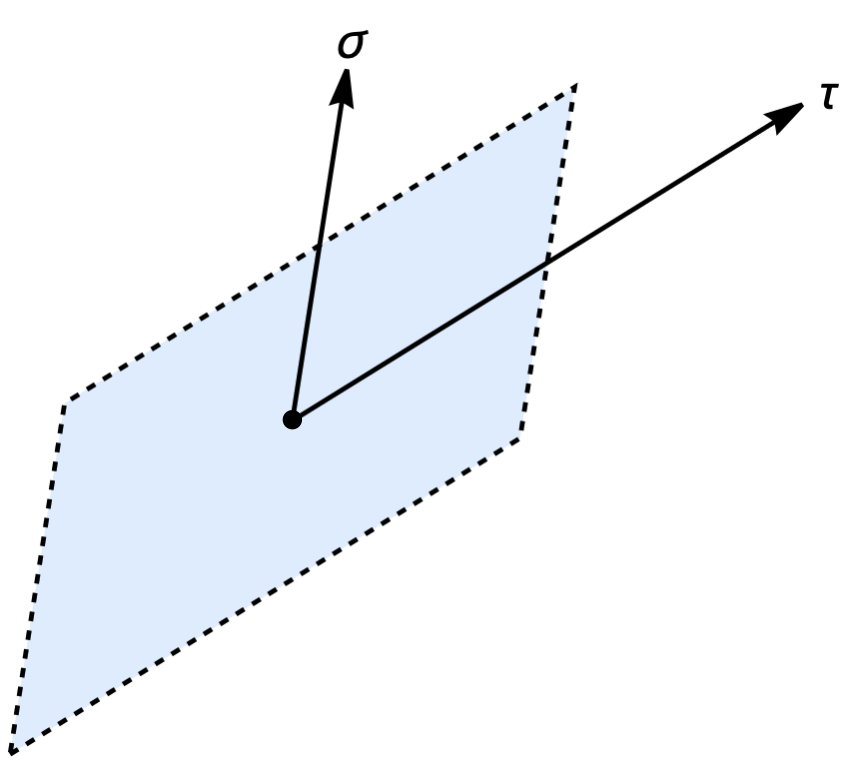
(a) $SU(N)$

(b) $SO(2N)$, $SO(2N+1)$, $Sp(N)$

Figure 1: $N$ eigenvalues are uniformly distributed in the colored region of the complex $u$ plane.

We now introduce our uniform parallelogram ansatz in the large $N$ limit. Specific form of the ansatz for each gauge node depends on the type of the gauge group. For $SU(N_{a})$ gauge nodes, the ansatz is given as Choi:2021rxi

$$u_{i}^{(a)}=\sigma x_{i}+\tau y_{i}\ ,\qquad x_{i},y_{i}\in\left(-\frac{1}{2},\frac{1}{2}\right)\ ,$$ (34)

with $\sum_{i=1}^{N_{a}}u_{i}^{(a)}=0$, and for $SO(2N_{a})$, $SO(2N_{a}+1)$ or $Sp(N_{a})$ gauge nodes, it is given by

$$u_{i}^{(a)}=\sigma x_{i}+\tau y_{i}\ ,\qquad x_{i}\in\left(0,\frac{1}{2}\right)\,,\;\;y_{i}\in\left(-\frac{1}{2},\frac{1}{2}\right)\ ,$$ (35)

where the eigenvalue $u_{i=1,2,\cdots,N_{a}}^{(a)}$’s are evenly distributed in the parallelogram for both cases as depicted in Figure 1. Note that we assumed $\textrm{Im}\left(\frac{\sigma}{\tau}\right)>0$ in (23). Next, let us introduce a $2$-dimensional eigenvalue density $\rho^{(a)}(x,y)$ given by

$$\rho^{(a)}(x,y)=\frac{1}{N_{a}}\sum_{i=1}^{N_{a}}\delta(x-x_{i})\delta(y-y_{i})\ ,\qquad\int dxdy\rho^{(a)}(x,y)=1\ ,$$ (36)

where the integration range is either (34) or (35). In the large $N_{a}$ limit, eigenvalues are densely distributed in the parallelogram (34), (35), so we can regard $\rho^{(a)}(x,y)$ as a continuous function. In particular, since eigenvalues are evenly distributed,

$$\rho^{(a)}(x,y)\to\left\{\begin{array}[]{ll}1\ ,&SU(N_{a})\\ 2\ ,&SO(2N_{a}),\;SO(2N_{a}+1),\;Sp(N_{a})\end{array}\right.\ ,$$ (37)

inside the parallelogram (34), (35), in the large $N_{a}$ continuum limit. Then, the summation over the eigenvalues can be approximated by the integration over $x,y$ with the uniform areal eigenvalue density $\rho^{(a)}(x,y)$ as follows:

$$\sum_{i=1}^{N_{a}}f(u^{(a)}_{i})\; \rightarrow\;N_{a}\int_{-1/2}^{1/2}\int_{-1/2}^{1/2}dxdy\;f(\sigma x+\tau y)+O(N_{a}^{0})\ ,$$ (38)

for $SU(N_{a})$ gauge nodes, and

$$\sum_{i=1}^{N_{a}}\left(f(u^{(a)}_{i})+f(-u^{(a)}_{i})\right)\; \rightarrow\;2N_{a}\int_{-1/2}^{1/2}\int_{-1/2}^{1/2}dxdy\;f(\sigma x+\tau y)+O(N_{a}^{0})\ ,$$ (39)

for $SO(2N_{a}),\,SO(2N_{a}+1),\,Sp(N_{a})$ gauge nodes. Here, we used the fact that there always exist pairs of positive/negative weights for $SO(2N_{a}),\,SO(2N_{a}+1),\,Sp(N_{a})$ gauge groups.

To show that the parallelogram ansatz (34), (35) indeed represents large $N$ saddle points of (21), we shall verify that each $v_{\sigma}(u_{ij}^{(ab)})$ and $v_{\tau}(u_{ij}^{(ab)})$ give vanishing force at the leading order $O(N^{1})$ within the parallelogram region (34), (35). Taking a derivative of the potential with respect to a particular eigenvalue $u_{i}^{(a)}$, we obtain

$$\sum_{j}\bigg{[}\frac{\partial}{\partial u_{i}^{(a)}}v_{\sigma}\big{(}u_{ij}^{(ab)}\big{)}+\frac{\partial}{\partial u_{i}^{(a)}}v_{\tau}\big{(}u_{ij}^{(ab)}\big{)}\bigg{]}=\pm\sum_{j}\bigg{[}\frac{1}{\sigma}\frac{\partial}{\partial x_{j}}v_{\sigma}\big{(}u_{ij}^{(ab)}\big{)}+\frac{1}{\tau}\frac{\partial}{\partial y_{j}}v_{\tau}\big{(}u_{ij}^{(ab)}\big{)}\bigg{]}\ ,$$ (40)

where we omitted possible overall normalization factor, which is irrelevant in the following discussion. Here, we used $\frac{\partial}{\partial u_{i}^{(a)}}=\pm\frac{\partial}{\partial u_{j}^{(b)}}$ and $u_{j}^{(b)}=\sigma x_{j}+\tau y_{j}$ so that the derivatives can be replaced by either $\frac{1}{\sigma}\frac{\partial}{\partial x_{j}}$ or $\frac{1}{\tau}\frac{\partial}{\partial y_{j}}$. The $\pm$ sign is fixed once we use one of the explicit expressions in (32) for $u_{ij}^{(ab)}$. In the large $N$ continuum limit, the above force becomes

$$N_{b}\int_{-1/2}^{1/2}\int_{-1/2}^{1/2}dx_{2}dy_{2}\left(\frac{1}{\sigma}\frac{\partial}{\partial x_{2}}v_{\sigma}\big{(}\sigma x_{12}+\tau y_{12}\big{)}+\frac{1}{\tau}\frac{\partial}{\partial y_{2}}v_{\tau}\big{(}\sigma x_{12}+\tau y_{12}\big{)}\right)\ ,$$ (41)

$$= \frac{N_{b}}{\sigma}\int_{-1/2}^{1/2}dy_{2}\;v_{\sigma}\big{(}\sigma x_{12}+\tau y_{12}\big{)}\Big{|}^{x_{2}=+1/2}_{x_{2}=-1/2}+\frac{N_{b}}{\tau}\int_{-1/2}^{1/2}dx_{2}v_{\tau}\big{(}\sigma x_{12}+\tau y_{12}\big{)}\Big{|}^{y_{2}=+1/2}_{y_{2}=-1/2}\ ,$$

where $x_{12}$ can be one of $x_{1}+x_{2}$, $-x_{1}-x_{2}$, $x_{1}-x_{2}$, $-x_{1}+x_{2}$, and so does $y_{12}$, in accordance with $u_{ij}^{(ab)}$. We see that both terms vanish when $v_{\sigma}$ and $v_{\tau}$ are periodic in $\sigma$ and $\tau$ respectively. Namely, the force-free condition is satisfied if

$$v_{\sigma}(z+\sigma)=v_{\sigma}(z)\ ,\quad v_{\tau}(z+\tau)=v_{\tau}(z)\ .$$ (42)

From (33), it is true that $e^{v_{\sigma}}$ and $e^{v_{\tau}}$ are indeed periodic in $\sigma,\tau$ respectively, due to the periodicity of $\Gamma$. When we have a fundamental chiral multiplet, the force-free condition is not met by our saddle. However, these terms are always subleading in $N$ (unless we take Veneziano-like limit of scaling the number of fundamentals) so that we ignore such contribution in the large $N$ limit.

Now it seems like we are done showing that our ansatz is indeed a saddle point of the integral. However, the periodicity of $v_{\sigma}$ and $v_{\tau}$ can be ruined if there exist a logarithmic branch point inside the integral domain (34), (35). Fortunately, we find that such branch points are absent in certain region of the parameter space for $\Delta_{I},\sigma,\tau$, which we shall study now. Let us first analyze $v_{\sigma}$. Absence of branch points requires that the following elliptic gamma function

$$\Gamma\left(-\frac{u_{12}+Q_{\chi}\cdot\Delta+1}{\sigma};-\frac{1}{\sigma},-\frac{\tau}{\sigma}\right)=\prod_{m,n=0}^{\infty}\frac{1-e^{2\pi i\left(\frac{u_{12}+Q_{\chi}\cdot\Delta+1}{\sigma}-\frac{m+1}{\sigma}-\frac{(n+1)\tau}{\sigma}\right)}}{1-e^{2\pi i\left(-\frac{u_{12}+Q_{\chi}\cdot\Delta+1}{\sigma}-\frac{m}{\sigma}-\frac{n\tau}{\sigma}\right)}}$$ (43)

has no zeros/poles from numerators/denominators for $u_{12}=\sigma x_{12}+\tau y_{12}$ in the region (34) or (35). To avoid poles from the denominator, we require

$$\Bigg{|}\exp\left[2\pi i\left(-\frac{u_{12}+Q_{\chi}\cdot\Delta+1}{\sigma}-\frac{m}{\sigma}-\frac{n\tau}{\sigma}\right)\right]\Bigg{|}<1\ ,\qquad\forall m,n\geq 0\ .$$ (44)

Note that $\imaginary\left[-\frac{u_{12}+Q_{\chi}\cdot\Delta+1}{\sigma}-\frac{m}{\sigma}-\frac{n\tau}{\sigma}\right]\geq\imaginary\left(-\frac{Q_{\chi}\cdot\Delta+1-\tau}{\sigma}\right)$, where the inequality is saturated at $m=n=0$ and $y_{12}=-1$. Hence, the above inequality holds if and only if

$$\imaginary\left(\frac{Q_{\chi}\cdot\Delta+1-\tau}{\sigma}\right)<0\ .$$ (45)

One can make a similar analysis for the other terms in $v_{\sigma}$ and $v_{\tau}$, which yields similar constraints as follows:

$$\begin{split}&\imaginary\left(\frac{1-\tau+Q_{\chi}\cdot\Delta}{\sigma}\right)<0\ ,\quad\imaginary\left(\frac{Q_{\chi}\cdot\Delta}{\sigma}\right)>0\ ,\\ &\imaginary\left(\frac{-\sigma+Q_{\chi}\cdot\Delta}{\tau}\right)>0\ ,\quad\imaginary\left(\frac{1+Q_{\chi}\cdot\Delta}{\tau}\right)<0\ .\end{split}$$ (46)

We should also demand the relation (46) to hold for the vector multiplets by inserting $Q_{\chi}=0$. Then, the second and the third conditions of (46) with $Q_{\chi}=0$ are automatically satisfied. The fourth condition also does not give any new constraint and simply means that the branch point exists exactly at the boundary of the parallelogram domain, which is acceptable. This is because no eigenvalues will be precisely at the boundary in the discrete picture.

One crucial problem is that if we insert $Q_{\chi}=0$ to the first condition of (46), it can never be satisfied since we are working in the region (23) where $\textrm{Im}\left(\frac{\sigma}{\tau}\right)>0$. The problematic term comes from the part of the vector multiplet contribution to $v_{\tau}$, which takes the following form:

$$\log\left(1-e^{2\pi i\left(\frac{\alpha_{a}(u)}{\tau}-\frac{m}{\tau}+\frac{n\sigma}{\tau}\right)}\right)\ .$$ (47)

When $m=n=0$, there indeed exist branch points at $\alpha_{a}(u)=0$. For the other $m,n$, there are no further branch points under (46). From now on, we shall separate the problematic Haar-measure-like factor, $m=n=0$ term of (47), from each gauge node, and redefine $V_{\tau}(u)$ as

$$e^{-V_{\tau}(u)}\quad\to\quad\prod_{a=1}^{n_{v}}\prod_{\alpha_{a}\in\Delta_{G_{a}}}\left(1-e^{2\pi i\frac{\alpha_{a}(u)}{\tau}}\right)\cdot e^{-\tilde{V}_{\tau}(u)}\ .$$ (48)

Finally, the matrix integral of the index (21) becomes

$$\mathcal{I}(\Delta,\sigma,\tau)=\frac{\kappa^{\textrm{rk}(G)}}{|W_{G}|}\oint\prod_{i=1}^{\textrm{rk}(G)}du_{i}\prod_{a=1}^{n_{v}}\prod_{\alpha_{a}\in\Delta_{G_{a}}}\left(1-e^{2\pi i\frac{\alpha_{a}(u)}{\tau}}\right)e^{-i\pi\mathbf{P}_{+}}e^{-V_{\sigma}(u)-\tilde{V}_{\tau}(u)}\ ,$$ (49)

where $V_{\sigma}$ and $\tilde{V}_{\tau}$ satisfy all the required periodicity (42) for vanishing force in the parallelogram (34), (35) under the assumption that the chemical potentials satisfy (46).

We next introduce the following integral identity

$$\begin{split}\frac{1}{|W_{G}|}&\oint_{\mathbb{T}^{\textrm{rk}(G)}}\prod_{i=1}^{\textrm{rk}(G)}du_{i}\prod_{\alpha\in\Delta_{G}^{+}}(1-e^{2\pi i\gamma\alpha(u)})(1-e^{-2\pi i\gamma\alpha(u)})\cdot f(u)\\ =&\oint_{\mathbb{T}^{\textrm{rk}(G)}}\prod_{i=1}^{\textrm{rk}(G)}du_{i}\prod_{\alpha\in\Delta_{G}^{+}}(1-e^{2\pi i\gamma\alpha(u)})\cdot f(u)\ ,\end{split}$$ (50)

where $\Delta_{G}^{+}$ denotes the set of all positive roots in $G$. This identity holds for any constant $\gamma$ and Weyl-invariant function $f(u)$ for a compact semisimple Lie group $G$. When $\gamma=1$, the right-hand side of this identity is widely used to reduce the computation complexity involving the Haar measure to the one only with half of the Haar measure. Our main claim is that the parallelogram ansatz (34), (35) solves the large $N$ saddle point problem after using the above identity to (49). To justify this, let us apply the identity with $\gamma=\frac{1}{\tau}$ as follows:

$$\mathcal{I}(\Delta,\sigma,\tau)=\kappa^{\textrm{rk}(G)}\oint\prod_{i=1}^{\textrm{rk}(G)}du_{i}\prod_{a=1}^{n_{v}}\prod_{\alpha_{a}\in\Delta^{+}_{G_{a}}}\left(1-e^{2\pi i\frac{\alpha_{a}(u)}{\tau}}\right)e^{-i\pi\mathbf{P}_{+}}e^{-V_{\sigma}(u)-\tilde{V}_{\tau}(u)}\ .$$ (51)

As an additional part of ansatz (34), (35), we order the eigenvalue $u_{i}^{(a)}$’s such that Choi:2021rxi

$$i<j\quad\Rightarrow\quad x_{i}>x_{j}\ .$$ (52)

Then, the half-Haar-measure-like factor has no zeros since

$$\left|e^{2\pi i\frac{\alpha_{a}(u)}{\tau}}\right|\ni\left|e^{2\pi i\frac{\sigma(x_{i}-x_{j})+\tau(y_{i}-y_{j})}{\tau}}\right|=\left|e^{2\pi i\frac{\sigma}{\tau}(x_{i}-x_{j})}\right|<1\$$ (53)

for positive roots ($i<j$) of $SU(N_{a})$ in (34), and

$$\left|e^{2\pi i\frac{\alpha_{a}(u)}{\tau}}\right|\ni\left\{\begin{array}[]{ll}\left|e^{2\pi i\frac{\sigma(x_{i}-x_{j})+\tau(y_{i}-y_{j})}{\tau}}\right|=\left|e^{2\pi i\frac{\sigma}{\tau}(x_{i}-x_{j})}\right|<1\\ \left|e^{2\pi i\frac{\sigma(x_{i}+x_{j})+\tau(y_{i}+y_{j})}{\tau}}\right|=\left|e^{2\pi i\frac{\sigma}{\tau}(x_{i}+x_{j})}\right|<1\end{array}\right.$$ (54)

for positive roots ($i<j$) of $SO(2N_{a})$, $SO(2N_{a}+1)$, $Sp(N_{a})$ in (35), when $\textrm{Im}\left(\frac{\sigma}{\tau}\right)>0$. Namely, the half-Haar-measure-like factor does not yield branch points to the potential of the index matrix model (51). This completes the proof that our ‘ordered’ parallelogram ansatz (34), (35) indeed solves the large $N$ saddle point equation of the index matrix integral (51) under the assumptions (16), (23), (46).

Another consequence of the above analysis is that the potentials (including the contribution from the half-Haar-measure-like factor) of (51) are periodic in $\sigma$ or $\tau$ and holomorphic in the ordered parallelogram region (34), (35). Therefore, upon evaluating the periodic integral in $\sigma$ or $\tau$ direction, they vanish at the parallelogram saddle point in the large $N$ continuum limit by Cauchy’s integral theorem in the leading $O(N^{2})$ order. Only the prefactor $\mathbf{P}_{+}$ contributes to the large $N$ free energy of the index (51).

Let us mention the case when our ansatz fails to become a valid saddle. When we have elementary fields whose $R$-charges scale as $O(1/N)$, the first condition of (46) can never be satisfied. This is because, in the large $N$ limit, we encounter dangerous terms of the form $\left(1-e^{2\pi i\frac{u_{ij}}{\tau}}\right)^{-1}$ just like the case of vector multiplet. However, in this case, such a dangerous term appears in the denominator, which cannot be removed using the identity (50) involving the Haar-measure-like factor. Thus, our ansatz does not solve the saddle point equation for the theories with ‘dense spectrum’ Agarwal:2019crm ; Agarwal:2020pol , which includes (the $\mathcal{N}=1$ gauge theory description of) a certain large $N$ limit of Argyres-Douglas theories Maruyoshi:2016aim ; Agarwal:2016pjo .

In summary, we have demonstrated that the uniform parallelogram ansatz (34) and (35) with the ordering (52) exactly solves the matrix model for the index (51) (and thus (13)) in the large $N$ limit, provided that the chemical potentials satisfy

$$\begin{split}&\sum_{I=1}^{d}\Delta_{I}-\sigma-\tau=-1\ ,\qquad\textrm{Im}\left(\frac{\sigma}{\tau}\right)>0\ ,\\ &\textrm{Im}\left(\frac{1+\sigma}{\tau}\right)<\imaginary\left(\frac{1+Q_{\chi}\cdot\Delta}{\tau}\right)<0<\imaginary\left(\frac{Q_{\chi}\cdot\Delta}{\sigma}\right)<\textrm{Im}\left(\frac{-1+\tau}{\sigma}\right)\ .\end{split}$$ (55)

As explained previously, the case with $\textrm{Im}\left(\frac{\sigma}{\tau}\right)<0$ can be studied by flipping the role of $\sigma$ and $\tau$ of the above case. If there exists the conjugate sector, it can be studied similarly where the chemical potentials satisfy

$$\begin{split}&\sum_{I=1}^{d}\Delta_{I}-\sigma-\tau=+1\ ,\qquad\textrm{Im}\left(\frac{\sigma}{\tau}\right)>0\ ,\\ &\textrm{Im}\left(\frac{1+\sigma}{\tau}\right)<\imaginary\left(\frac{Q_{\chi}\cdot\Delta}{\tau}\right)<0<\imaginary\left(\frac{-1+Q_{\chi}\cdot\Delta}{\sigma}\right)<\textrm{Im}\left(\frac{-1+\tau}{\sigma}\right)\ ,\end{split}$$ (56)

or its $\sigma\leftrightarrow\tau$ flipped version. One can also take the collinear limit, in which $\textrm{Im}\left(\frac{\sigma}{\tau}\right)\to 0$, from both cases smoothly. If both sectors (55), (56) exist, upon Legendre transformation of the free energy to the microcanonical ensemble, they give complex conjugate contributions, thereby realizing the oscillating signs of the index degeneracy Agarwal:2020zwm ; Choi:2020baw . The constraints (55), (56) are reminiscent of the stability conditions of the Euclidean BPS black hole solutions against the condensation of the D3-brane instantons Aharony:2021zkr . It would be interesting to study the relation between them if any.

In any case, the resulting large $N$ free energy of the index (13) is given by

$$\log\mathcal{I} =-\frac{i\pi}{24\sigma\tau}\left[\sum_{I,J,K=1}^{d}\!\!\Tr(Q^{I}Q^{J}Q^{K})\Delta_{I}\Delta_{J}\Delta_{K}-(\sigma^{2}+\tau^{2}+1)\sum_{I=1}^{d}\Tr(Q^{I})\Delta_{I}\right]+O(N)$$

$$\sim-\frac{i\pi}{24\sigma\tau}\sum_{I,J,K=1}^{d}\Tr(Q^{I}Q^{J}Q^{K})\Delta_{I}\Delta_{J}\Delta_{K}\ ,$$ (57)

where we only kept terms of order $O(N^{2})$ from the prefactor $-i\pi\mathbf{P}_{\pm}$. We can drop the second term in the first line of (2.2) for the gauge theories of our interest, where $\textrm{rk}(G_{a})=O(N)$, since one can show that $\Tr(Q^{I})=O(N^{1})$ or $O(N^{0})$ at large $N$ as follows:

$$\Tr(Q^{I}) =\frac{1}{2}\sum_{a}\left[\dim(G_{a})+\sum_{\chi_{a}}(2Q^{I}_{\chi_{a}}-1)\dim(\mathcal{R}_{\chi_{a}})\right]$$ (58)

$$=\frac{1}{2}\sum_{a}\textrm{rk}(G_{a})\left(d_{2}(G_{a})+\sum_{\chi_{a}}(2Q_{\chi_{a}}^{I}-1)d_{2}(\mathcal{R}_{\chi_{a}})\right)+O(N)$$

$$=\sum_{a}\textrm{rk}(G_{a})\Tr(Q^{I}G_{a}G_{a})+O(N)$$

$$=O(N)\ ,$$

where the second line comes from the fact that for the rank-2 tensor representations $d_{2}(\mathcal{R})/\dim(\mathcal{R})\sim 1/N$ at large $N$. In the third line, we find the leading order term vanishes since $Q^{I}$-symmetry is anomaly-free.

As a concrete holographic example, let us consider the 4d $\mathcal{N}=1$ SCFT describing the low energy dynamics of a stack of $N$ D3-branes probing a conical Calabi-Yau 3-fold singularity. This theory is dual to type IIB string theory on AdS${}_{5}\times$ SE₅, where SE₅ is the Sasaki-Einstein 5-manifold serving as the base of the Calabi-Yau 3-fold. Then, the above formula can be written as

$$\begin{split}\log\mathcal{I}(\Delta,\sigma,\tau)\sim-\frac{i\pi N^{2}}{24\sigma\tau}\sum_{I,J,K=1}^{d}C^{IJK}\Delta_{I}\Delta_{J}\Delta_{K}\ ,\end{split}$$ (59)

where $C^{IJK}\equiv\frac{1}{N^{2}}\Tr(Q^{I}Q^{J}Q^{K})$’s correspond to the Chern-Simons couplings of the 5d $\mathcal{N}=1$ gauged supergravity, which can be obtained from a consistent Kaluza-Klein truncation of type IIB supergravity on $\textrm{SE}_{5}$. This precisely matches the entropy function of the BPS black holes in AdS${}_{5}\times\textrm{SE}_{5}$ Hosseini:2017mds ; Hosseini:2018dob ; Cabo-Bizet:2018ehj ; Cassani:2019mms ; Lanir:2019abx ; Amariti:2019mgp ; Benini:2020gjh , thus accounting for their microstates.

One may want to rewrite (2.2) in terms of the superconformal $R$-symmetry chemical potential $\delta=\frac{\sigma+\tau-1}{2}$ and flavor symmetry chemical potential $\delta^{I}$’s. Note that $\Delta_{I}$’s in (2.2) are all in fact integer-shifted ones $\tilde{\Delta}_{I}=\Delta_{I}+n_{I}p_{I}$’s as explained in Section 2.1. Using the linear maps around (8) between charges and chemical potentials, we get

$$\begin{split}\log\mathcal{I}\sim-\frac{i\pi}{24\sigma\tau}&\left[k_{RRR}\,\delta_{\mp}^{3}+3\sum_{I=1}^{d-1}k_{RRI}\,\delta_{\mp}^{2}\tilde{\delta}^{I}+3\sum_{I,J=1}^{d-1}k_{RIJ}\,\delta_{\mp}\tilde{\delta}^{I}\tilde{\delta}^{J}+\sum_{I,J,K=1}^{d-1}k_{IJK}\tilde{\delta}^{I}\tilde{\delta}^{J}\tilde{\delta}^{K}\right]\ ,\end{split}$$ (60)

where $\delta_{\mp}\equiv\frac{\sigma+\tau\mp 1}{2}$, and $\tilde{\delta}^{I}\equiv\delta^{I}+\sum_{J=1}^{d}n_{J}p_{J}\xi^{JI}$ with $\sum_{I=1}^{d}n_{I}p_{I}=0$ for $\delta_{-}$ and 2 for $\delta_{+}$. Various trace anomaly coefficients in the above formula are defined as

$$\begin{split}k_{RRR}&\equiv\Tr R^{3}=\textrm{dim}(G)+\sum_{\chi}\dim(\mathcal{R}_{\chi})(R_{\chi}-1)^{3}=\frac{16}{9}(5a-3c)\ ,\\ k_{RRI}&\equiv\Tr R^{2}f_{I}=\sum_{\chi}\dim(\mathcal{R}_{\chi})(R_{\chi}-1)^{2}f_{\chi,I}\ ,\\ k_{RIJ}&\equiv\Tr Rf_{I}f_{J}=\sum_{\chi}\dim(\mathcal{R}_{\chi})(R_{\chi}-1)f_{\chi,I}f_{\chi,J}\ ,\\ k_{IJK}&\equiv\Tr f_{I}f_{J}f_{K}=\sum_{\chi}\dim(\mathcal{R}_{\chi})f_{\chi,I}f_{\chi,J}f_{\chi,K}\ .\end{split}$$ (61)

Here, $R_{\chi}$ and $f_{\chi,I}$’s are the superconformal $R$ and flavor charges of (the scalar in) the chiral multiplet $\Phi_{\chi}$, and $a,c$ are the central charges or conformal anomalies of the theory.

If we turn off all the shifted flavor chemical potential $\tilde{\delta}^{I}$’s in (60); e.g. $\delta^{I}=n_{I}=0$ for the case with $\delta_{-}$, we obtain a universal large $N$ formula for the index of 4d $\mathcal{N}=1$ SCFTs given by

$$\begin{split}\log\mathcal{I}(\sigma,\tau)&\sim-\Tr R^{3}\;\frac{i\pi\delta_{\mp}^{3}}{24\sigma\tau}=-(5a-3c)\;\frac{2i\pi\delta_{\mp}^{3}}{27\sigma\tau}\ ,\end{split}$$ (62)

where $\delta_{\mp}=\frac{\sigma+\tau\mp 1}{2}$. One nice fact in this unrefined case is that if we take the collinear limit $\textrm{Im}(\frac{\sigma}{\tau})\to 0$, the conditions (55), (56) are trivially satisfied. Namely, the above large $N$ formula works for arbitrary collinear $\sigma,\tau$ when the shifted flavor chemical potentials are all turned off. For holographic theories, we have $a,\,c=O(N^{2})$ and $a-c=O(N^{1})$ or $O(N^{0})$. Then, the above formula accounts for the Bekenstein-Hawking entropy of the universal BPS black holes in AdS₅ Gutowski:2004ez ; Gutowski:2004yv ; Chong:2005hr ; Kunduri:2006ek , arising as a solution of 5d minimal gauged supergravity whose Newton constant $G_{N}$ and gauge coupling $g$ are related to $c$ as $\frac{\pi^{2}}{g^{3}G_{N}}=c$ at $O(N^{2})$.

2.3 More general saddles

In this subsection, we shall construct two kinds of new large $N$ saddle points generalizing the parallelogram ansatz (34), (35). The first one is $(\sigma_{r_{1}},\tau_{r_{2}})$-saddles whose edge vectors of the parallelogram ansatz (34), (35) are now given by Choi:2021rxi

$$(\sigma_{r_{1}},\tau_{r_{2}})\equiv(\sigma+r_{1},\tau+r_{2})\ ,$$ (63)

where $r_{1},r_{2}\in\mathbb{Z}$. Since $\Gamma(z;\sigma,\tau)=\Gamma(z;\sigma+1,\tau)=\Gamma(z;\sigma,\tau+1)$, one can do the very same analysis in the former subsection with $(\sigma_{r_{1}},\tau_{r_{2}})$. Then, we again perform appropriate shift of $\Delta_{I}$’s such that shifted chemical potentials $\Delta_{I}^{(r_{1},r_{2})},\;\sigma_{r_{1}},\;\tau_{r_{2}}$ satisfy (16), i.e.

$$\sum_{I=1}^{d}\Delta_{I}^{(r_{1},r_{2})}-\sigma_{r_{1}}-\tau_{r_{2}}=\mp 1\ .$$ (64)

For given $\Delta_{I},\sigma,\tau$, there may or may not exist the possible shift of $\Delta_{I}$’s satisfying the above condition and (55), (56) depending on the period $p_{I}$’s and $(r_{1},r_{2})$. In principle, allowed $(r_{1},r_{2})$ can be determined for given $\Delta_{I},\sigma,\tau$, but in general, it depends on the explicit details of the theory, which will not be discussed here. However, for the simplest case when $\sigma=\tau$ and all the flavor chemical potentials are turned off, one can show that only the cases with $r_{1}=r_{2}$ are allowed Choi:2021rxi ; Choi:2022asl . When the above condition and (55), (56) are satisfied, the $(\sigma_{r_{1}},\tau_{r_{2}})$-saddles contribute to the index in the large $N$ limit as

$$\log\mathcal{I}\sim-\frac{i\pi}{24\sigma_{r_{1}}\tau_{r_{2}}}\sum_{I,J,K=1}^{d}\Tr(Q^{I}Q^{J}Q^{K})\Delta_{I}^{(r_{1},r_{2})}\Delta_{J}^{(r_{1},r_{2})}\Delta_{K}^{(r_{1},r_{2})}\ .$$ (65)

One can easily show that after the Legendre transformation, their leading large $N$ entropies are all the same Choi:2021rxi . In dual AdS₅ gravity side, these saddles will correspond to multiple Euclidean solutions coming from the same Lorentzian BPS black hole solution after compactifying the temporal circle, which are explicitly constructed in asymptotically AdS${}_{5}\times S^{5}$ case Aharony:2021zkr .

Next, we construct multi-cut saddle points in the collinear case $\textrm{Im}\left(\frac{\sigma}{\tau}\right)=0$. Our $K$-cut ansatz roughly takes the following form in the large $N$ continuum limit Choi:2021rxi :

$$u_{A}^{(a)}(x,y)=\frac{A}{K}+\sigma x+\tau y\ ,$$ (66)

where $A=0,1,\cdots,K-1$ labels $K$ clusters of evenly distributed eigenvalues forming the $K$-cuts. Domain of $(x,y)$ should be properly given according to the gauge group at each node as (34), (35). Although these cuts are linear (not areal), we again adopt the $2$-parameter labeling of eigenvalues with uniform $2$-dimensional distributions. One can understand it as the collinear limit $\textrm{Im}\left(\frac{\sigma}{\tau}\right)\to 0$ of the areal distribution. Each cut contains evenly distributed $\frac{N}{K}$ eigenvalues so the density function is given by

$$\rho_{A}^{(a)}(x,y)\to\left\{\begin{array}[]{ll}\frac{1}{K}\ ,&SU(N_{a})\\ \frac{2}{K}\ ,&SO(2N_{a}),\;SO(2N_{a}+1),\;Sp(N_{a})\end{array}\right.\ .$$ (67)

Now, let us denote the index (13) schematically as $\mathcal{I}=\frac{\kappa^{N}}{|W_{G}|}\oint d^{N}u\;e^{-V(u)}$. Each chiral multiplet $\Phi_{\chi}$ contributes to the force acting on a particular eigenvalue $u_{A}^{(a)}(x_{i},y_{i})$ as

$$\sum_{j}\sum_{A=0}^{K-1}\frac{\partial}{\partial u_{i}^{(a)}}\log\Gamma\left(u_{ij}^{(ab)}+\frac{A}{K}+Q_{\chi}\cdot\Delta;\sigma,\tau\right)\ ,$$ (68)

where $u_{ij}^{(ab)}$ denotes one of (32) and $u_{i}^{(a)}$ takes the value from the parallelogram ansatz (34), (35) as before. Once again, the vector multiplet contribution can be understood with overall minus sign, and identifying $u_{ij}^{(aa)}=\alpha_{a}(u)$ and $Q_{\chi}=(0,0,\cdots,0)$. Using the following identity

$$\sum_{A=0}^{K-1}\log\Gamma\left(z+\frac{A}{K};\sigma,\tau\right)=\log\Gamma(Kz;K\sigma,K\tau)\ ,$$ (69)

above formula is simplified as

$$K\sum_{j}\frac{\partial}{\partial{u_{i}^{(a)}}^{\prime}}\log\Gamma\left({u_{ij}^{(ab)}}^{\prime}+Q_{\chi}\cdot\Delta^{\prime};\sigma^{\prime},\tau^{\prime}\right)\ ,$$ (70)

where $\Delta_{I}^{\prime}\equiv K\Delta_{I}+n_{I}^{(K)}p_{I}$, $\sigma^{\prime}\equiv K\sigma$, $\tau^{\prime}\equiv K\tau$, and ${u_{i}^{(a)}}^{\prime}\equiv Ku_{i}^{(a)}$. Here, $n_{I}^{(K)}\in\mathbb{Z}$ are appropriate integer shifts of $K\Delta_{I}$’s so that

$$\sum_{I=1}^{d}\Delta_{I}^{\prime}-\sigma^{\prime}-\tau^{\prime}=\mp 1\ .$$ (71)

Such shifts may or may not exist depending on $p_{I}$’s. The above force takes ($K$ times) the precisely same form with that of the 1-cut solution with $\Delta_{I}^{\prime},\sigma^{\prime},\tau^{\prime}$ before the $SL(3,\mathbb{Z})$ transformation. Therefore, our $K$-cut ansatz (66) indeed represents large $N$ saddles generalizing 1-cut solution (34), (35) if $\Delta_{I}^{\prime},\sigma^{\prime},\tau^{\prime}$ satisfy the above condition and (55), (56). Then, it is straightforward to show that each chiral multiplet $\Phi_{\chi}$ contributes to $V(u)$ as

$$v(u_{ij}^{(ab)})=-K\sum_{i,j}\log\Gamma\left(Ku_{ij}^{(ab)}+Q_{\chi}\cdot(K\Delta);K\sigma,K\tau\right)$$ (72)

$$\xrightarrow{N\to\infty}-\frac{N_{a}N_{b}}{K}\int_{-1/2}^{1/2}\int_{-1/2}^{1/2}\int_{-1/2}^{1/2}\int_{-1/2}^{1/2}dx_{1}dy_{1}dx_{2}dy_{2}\log\Gamma\left(u^{\prime}_{12}+Q_{\chi}\cdot\Delta^{\prime};\sigma^{\prime},\tau^{\prime}\right)\ ,$$

where $u^{\prime}_{12}\equiv\sigma^{\prime}x_{12}+\tau^{\prime}y_{12}$. Here, we used the periodicity $\Gamma(z+1;\sigma,\tau)=\Gamma(z;\sigma,\tau)$ to reduce the double sum over cuts to the single sum. Vector multiplet contribution can be treated as before. The above potential is the same as $\frac{1}{K}$ times that of the 1-cut solution with primed variables. As a result, the $K$-cut solution contributes to the large $N$ free energy as

$$\log\mathcal{I}\sim-\frac{i\pi}{24K\sigma^{\prime}\tau^{\prime}}\sum_{I,J,K=1}^{d}\Tr(Q^{I}Q^{J}Q^{K})\Delta_{I}^{\prime}\Delta_{J}^{\prime}\Delta_{K}^{\prime}\ ,$$ (73)

whose leading large $N$ entropy, after the Legendre transformation, is $\frac{1}{K}$ times that of the 1-cut solution Choi:2021rxi . In dual AdS₅ gravity side, these saddles will be dual to $\mathbb{Z}_{K}$ orbifolds of the Euclidean BPS black hole solutions dual to the 1-cut solution, which are explicitly constructed in asymptotically AdS${}_{5}\times S^{5}$ case Aharony:2021zkr .

One can also combine the above two saddles to make more general saddles. Then, their contributions to the index will be

$$\log\mathcal{I}\sim-\frac{i\pi}{24K\sigma^{\prime}_{r_{1}}\tau^{\prime}_{r_{2}}}\sum_{I,J,K=1}^{d}\Tr(Q^{I}Q^{J}Q^{K}){\Delta_{I}^{\prime}}^{(r_{1},r_{2})}{\Delta_{J}^{\prime}}^{(r_{1},r_{2})}{\Delta_{K}^{\prime}}^{(r_{1},r_{2})}\ ,$$ (74)

where $\sigma^{\prime}_{r_{1}}\equiv K\sigma+r_{1}$, $\tau^{\prime}_{r_{2}}\equiv K\tau+r_{2}$, and ${\Delta_{I}^{\prime}}^{(r_{1},r_{2})}\equiv K\Delta_{I}+n_{I}^{(K,r_{1},r_{2})}p_{I}$ satisfy

$$\sum_{I=1}^{d}{\Delta_{I}^{\prime}}^{(r_{1},r_{2})}-{\sigma^{\prime}}_{r_{1}}-{\tau^{\prime}}_{r_{2}}=\mp 1\ ,$$ (75)

and (55) or (56) for $n_{I}^{(K,r_{1},r_{2})}\in\mathbb{Z}$. In principle, we should sum over contributions from all of these saddles labeled by $(K,r_{1},r_{2},\mp)$ as the large $N$ approximation of the index. However, it is not known whether this sum is convergent. Also, it is not known if all the contributions should be summed with equal weights within the framework of the Picard-Lefschetz theory. Here, we just state that we have a one-to-one correspondence between these kinds of large $N$ saddles for $\mathcal{N}=4$ $U(N)$ SYM Choi:2021rxi and (orbifolded) Euclidean black hole solutions in AdS${}_{5}\times S^{5}$ Aharony:2021zkr . Further, note that they are also in one-to-one correspondence with the large $N$ limit of the Hong-Liu solutions Hong:2018viz of the Bethe Ansatz Equation for the index of $\mathcal{N}=4$ $SU(N)$ SYM Benini:2018ywd .

Let us make a final comment before closing this section. In Choi:2021rxi , multi-cut saddle points with unequal filling fractions were found in $\mathcal{N}=4$ $U(N)$ SYM. Here, unequal filling fractions mean that the number of eigenvalues occupying each parallelogram is different. Neither corresponding solutions in AdS₅ gravity nor Bethe roots of the index are known. It would be interesting to construct this kind of large $N$ solutions for $\mathcal{N}=1$ gauge theories, generalizing the multi-cut saddle points in this subsection. Since such solutions highly depend on the details of the theory, we shall not discuss them here.

3 Examples

In this section, we invoke the large $N$ analysis in Section 2 against several concrete holographic models. For brevity, we will omit all the modular parameters of the elliptic gamma functions in the following examples, regardless of whether they have been $SL(3,\mathbb{Z})$ transformed or not.

3.1 Klebanov-Witten theory

The Klebanov-Witten theory Klebanov:1998hh is a 4d $\mathcal{N}=1$ supersymmetric gauge theory, which arises as a low-energy description of a stack of $N$ D3-branes sitting at a conifold singularity. This theory is dual to type IIB string theory on AdS${}_{5}\times T^{1,1}$.

The theory has $SU(N)\times SU(N)$ gauge group with two pairs of bifundamental chiral multiplets $A_{1,2},B_{1,2}$ transforming in the $(\mathbf{N},\overline{\mathbf{N}})$ and $(\overline{\mathbf{N}},\mathbf{N})$ representations. The quartic superpotential is given by

$$\mathcal{W}=\tr\big(A_{1}B_{1}A_{2}B_{2}-A_{1}B_{2}A_{2}B_{1})\ .$$ (76)

Apart from the conformal symmetry, the bosonic global symmetry of the theory involves the $R$-symmetry, two $SU(2)$ flavor symmetries rotating the $A_{1,2}$ and $B_{1,2}$ doublets, and a $U(1)_{B}$ baryonic symmetry as follows:

$$U(1)_{R}\times U(1)_{B}\times SU(2)_{F_{1}}\times SU(2)_{F_{2}}\ .$$ (77)

The charge of each multiplet under the maximal torus of the global symmetry is presented in Table 1. In general, the $R$-charge $R_{0}$, determined by the anomaly-free condition and $R[\mathcal{W}]=2$, must be considered as candidate $R$-charge. However, for the Klebanov-Witten theory, it becomes the true $R$-charge as $U(1)_{B}$ is enhanced to $SU(2)_{B}$ at IR.

	$U(1)_{F_{1}}$	$U(1)_{F_{2}}$	$U(1)_{B}$	$U(1)_{R_{0}}$	$U(1)_{1}$	$U(1)_{2}$	$U(1)_{3}$	$U(1)_{4}$
$A_{1}$	$1$	$0$	$1$	$1/2$	$1$	$0$	$0$	$0$
$A_{2}$	$-1$	$0$	$1$	$1/2$	$0$	$1$	$0$	$0$
$B_{1}$	$0$	$1$	$-1$	$1/2$	$0$	$0$	$1$	$0$
$B_{2}$	$0$	$-1$	$-1$	$1/2$	$0$	$0$	$0$	$1$

Table 1: Charge assignment of each chiral multiplet in the Klebanov-Witten theory

For clarification, let us begin with the usual definition of the superconformal index with the $(-1)^{F}$ insertion

$$\mathcal{I}(\xi,\sigma,\tau)=\Tr\left[(-1)^{F}e^{2\pi i\sigma\left(J_{1}+\frac{R}{2}\right)}e^{2\pi i\tau\left(J_{2}+\frac{R}{2}\right)}e^{2\pi i\left(\xi_{F_{1}}Q_{F_{1}}+\xi_{F_{2}}Q_{F_{2}}+\xi_{B}Q_{B}\right)}\right]\ .$$ (78)

As explained thoroughly in section 2, it is convenient to redefine the flavor chemical potentials in terms of

$$\begin{split}\Delta_{1}&=\xi_{F_{1}}+\xi_{B}+\frac{1}{4}(\tau+\sigma\mp 1)\ ,\qquad\Delta_{2}=-\xi_{F_{1}}+\xi_{B}+\frac{1}{4}(\tau+\sigma\mp 1)\ ,\\ \Delta_{3}&=\xi_{F_{2}}-\xi_{B}+\frac{1}{4}(\tau+\sigma\mp 1)\ ,\qquad\Delta_{4}=-\xi_{F_{2}}-\xi_{B}+\frac{1}{4}(\tau+\sigma\mp 1)\ ,\end{split}$$ (79)

which satisfy the following relation:

$$\Delta_{1}+\Delta_{2}+\Delta_{3}+\Delta_{4}=\tau+\sigma\mp 1\ .$$ (80)

Then, the index takes a more transparent form of (11):

$$\mathcal{I}(\Delta,p,q)=\Tr\left[e^{2\pi i\sigma J_{1}}e^{2\pi i\tau J_{2}}\prod_{I=1}^{4}e^{2\pi i\Delta_{I}Q^{I}}\right]\ ,$$ (81)

where new charge $Q^{I}$’s are integer-normalized as in Table 1. Here, we have assigned chemical potential $\Delta_{I}$’s to each bifundamental fields. In other words, since $2Q^{I}$ plays the role of $R$-symmetry, there is one-to-one correspondence between bifundamental field and its $R$-symmetry, like $\mathcal{N}=4$ SYM case. Now we can write the integral representation of the index (81) as

$$\begin{split}\mathcal{I}(\Delta,\sigma,\tau)=&\frac{\kappa^{2N}}{(N!)^{2}}\oint\prod_{i=1}^{N}du_{i}^{(1)}du_{i}^{(2)}\frac{1}{\prod_{i\neq j}^{N}\Gamma\Big{(}u_{ij}^{(11)}\Big{)}\Gamma\Big{(}u_{ij}^{(22)}\Big{)}}\\ &\times\prod_{i,j=1}^{N}\Gamma\Big{(}u_{ij}^{(12)}+\Delta_{1}\Big{)}\Gamma\Big{(}u_{ij}^{(12)}+\Delta_{2}\Big{)}\Gamma\Big{(}u_{ij}^{(21)}+\Delta_{3}\Big{)}\Gamma\Big{(}u_{ij}^{(21)}+\Delta_{4}\Big{)}\ ,\end{split}$$ (82)

where $u_{ij}^{(ab)}\equiv u_{i}^{(a)}-u_{j}^{(b)}$.

Using the $SL(3,\mathbb{Z})$ identity (18) assuming $\textrm{Im}\left(\frac{\sigma}{\tau}\right)>0$, the above integrand becomes

$$\mathcal{I}(\Delta,\sigma,\tau)=\frac{\kappa^{2N}}{(N!)^{2}}\oint\prod_{i=1}^{N}du_{i}^{(1)}du_{i}^{(2)}e^{-i\pi\mathbf{P}_{+}}e^{-\sum_{i,j=1}^{N}\big{(}V_{\sigma}(u)+V_{\tau}(u)\big{)}}\ ,$$ (83)

where (ignoring $i=j$ terms of the vector multiplet contribution)

$$V_{\sigma}(u) \equiv\frac{1}{2}\sum_{I=1}^{4}\log\Gamma\left(-\frac{u_{ij}^{(12)}+\Delta_{I}+1}{\sigma}\right)-\frac{1}{2}\log\Gamma\left(-\frac{u_{ij}^{(11)}+1}{\sigma}\right)-\frac{1}{2}\log\Gamma\left(-\frac{u_{ij}^{(22)}+1}{\sigma}\right)$$

$$\qquad+(u\rightarrow-u)\ ,$$ (84)

$$V_{\tau}(u) \equiv\frac{1}{2}\sum_{I=1}^{4}\log\Gamma\left(\frac{u_{ij}^{(12)}+\Delta_{I}+1}{\tau}\right)-\frac{1}{2}\log\Gamma\left(\frac{u_{ij}^{(11)}}{\tau}\right)-\frac{1}{2}\log\Gamma\left(\frac{u_{ij}^{(22)}}{\tau}\right)$$

$$\qquad+(u\rightarrow-u)\ .$$

For convenience, we averaged over the contributions from positive and negative roots and weights to have even function of $u$, which is true for the Klebanov-Witten theory. Then, the cubic and linear terms in $u$ of the prefactor are automatically cancelled, and hence we obtain

$$\begin{split}-i&\pi\mathbf{P}_{\pm}\Big{|}_{\eqref{eqn: two relevant branches of KW theory}}\\ =&-\frac{i\pi}{2}\Bigg{[}\sum_{i,j=1}^{N}\sum_{I=1}^{4}P_{\pm}(u_{ij}^{(12)}+\Delta_{I})-\sum_{i\neq j}^{N}P_{\pm}(u_{ij}^{(11)})-\sum_{i\neq j}^{N}P_{\pm}(u_{ij}^{(22)})\Bigg{]}+(u\rightarrow-u)\\ =&-\frac{i\pi N^{2}(\Delta_{1}\Delta_{2}\Delta_{3}+\Delta_{1}\Delta_{2}\Delta_{4}+\Delta_{1}\Delta_{3}\Delta_{4}+\Delta_{2}\Delta_{3}\Delta_{4})}{\sigma\tau}\\ &-\frac{i\pi N(\sigma+\tau-\sigma\tau)}{6\sigma\tau}(\Delta_{1}+\Delta_{2}+\Delta_{3}+\Delta_{4})\\ &+\frac{i\pi(\sigma+\tau\mp 1)}{2\sigma\tau}\left[\sum_{i,j=1}^{N}2(u_{ij}^{(12)})^{2}-\sum_{i\neq j}^{N}(u_{ij}^{(11)})^{2}-\sum_{i\neq j}^{N}(u_{ij}^{(22)})^{2}\right]\ .\end{split}$$ (85)

From the discussion in section 2, we recognize that the $u$-dependent part can be rewritten as

$$\sum_{i,j=1}^{N}\big{[}2(u_{ij}^{(12)})^{2}-(u_{ij}^{(11)})^{2}-(u_{ij}^{(22)})^{2}\big{]} =\big{(}2d_{2}(\mathbf{N})\dim(\overline{\mathbf{N}})+2\dim(\mathbf{N})d_{2}(\overline{\mathbf{N}})-2d_{2}(\textrm{Adj})\big{)}|u|^{2}$$

$$=\left(4\cdot\frac{1}{2}\cdot N-2N\right)|u|^{2}=0\ ,$$ (86)

since $2Q^{I}-1=1$. In addition, since the overall gauge group is $SU(N)\times SU(N)$, we only need to use the first type of parallelogram ansatz (34) to solve the large $N$ matrix model. In doing so, we should split the dangerous Haar-measure-like factor from each gauge node, and then use the integral identity (50). This leads to

$$\mathcal{I}(\Delta,\sigma,\tau)=\kappa^{2N}\oint\prod_{c=1}^{2}\prod_{i=1}^{N}du_{i}^{(c)}\prod_{i<j}^{N}\left(1-e^{\frac{2\pi iu_{ij}^{(cc)}}{\tau}}\right)e^{-i\pi\mathbf{P}_{+}}e^{-\sum_{i,j=1}^{N}\big{(}V_{\sigma}(u)+\tilde{V}_{\tau}(u)\big{)}}\ ,$$ (87)

where both $V_{\sigma},\tilde{V}_{\tau}$ and the factorized half-Haar-measure-like factor have vanishing force within the parallelogram region if the following constraints (46) are met:

$$\imaginary\left(\frac{1-\tau+\Delta_{I}}{\sigma}\right)<0,\;\imaginary\left(\frac{\Delta_{I}}{\sigma}\right)>0,\;\imaginary\left(\frac{-\sigma+\Delta_{I}}{\tau}\right)>0,\;\imaginary\left(\frac{1+\Delta_{I}}{\tau}\right)<0\ .$$ (88)

It also follows that the potentials $V_{\sigma},\tilde{V}_{\tau}$ themselves vanish at the parallelogram saddle point at leading $O(N^{2})$ order. Consequently, the only terms that contribute to the free energy is the $u$-independent part of the prefactor $-i\pi\mathbf{P}_{\pm}$, which has the same structure as (2.2):

$$\begin{split}\log\mathcal{I}(\Delta,\sigma,\tau)\sim&-\frac{i\pi N^{2}(\Delta_{1}\Delta_{2}\Delta_{3}+\Delta_{1}\Delta_{2}\Delta_{4}+\Delta_{1}\Delta_{3}\Delta_{4}+\Delta_{2}\Delta_{3}\Delta_{4})}{\tau\sigma}\ ,\end{split}$$ (89)

where we only kept terms of order $O(N^{2})$. This perfectly matches the entropy function of the BPS black holes in AdS${}_{5}\times T^{1,1}$, which was obtained in the gravity side when $\sigma=\tau$ and only the chemical potentials for the $R$-symmetry $U(1)_{R}$ and baryonic symmetry $U(1)_{B}$ are turned on Benini:2020gjh .

3.2 $Y^{p,q}$-theories

Let us consider the low energy dynamics of a stack of D3-branes probing a nontrivial toric Calabi-Yau 3-fold singularity. As a concrete example, we will study an infinite family of $\mathcal{N}=1$ quiver gauge theories dual to type IIB string theory on AdS${}_{5}\times Y^{p,q}$, where $p>q$ are positive integers Martelli:2004wu ; Benvenuti:2004dy . $Y^{p,q}$’s are one of the well-known examples of the toric Sasaki-Einstein 5-manifolds.

The theory has $2p$ $SU(N)$ gauge nodes with $4p+2q$ bifundamental chiral multiplets categorized by four types: $p$ fields of type $U_{1,2}$, $q$ fields of type $V_{1,2}$, $p-q$ fields of type $Z$, and $p+q$ fields of type $Y$. The superpotential is then made by summing over all possible cubic and quartic gauge invariant operators using $U_{\alpha},V_{\alpha},Y$ and $Z$ as follows:

$$\mathcal{W}=\sum_{k}\epsilon^{\alpha\beta}\tr\big(U_{\alpha}^{(k)}V_{\beta}^{(k)}Y^{(2k+2)}+V_{\alpha}^{(k)}U_{\beta}^{(k+1)}Y^{(2k+3)}\big{missing})+\sum_{k}\epsilon^{\alpha\beta}\tr\big(Z^{(k)}U_{\alpha}^{(k+1)}Y^{(2k+3)}U_{\beta}^{(k)}\big{missing})\ .$$ (90)

In addition to the conformal symmetry, the global symmetry of the theory is given as

$$U(1)_{R}\times U(1)_{B}\times U(1)_{F_{1}}\times SU(2)_{F_{2}}\ ,$$ (91)

whose charge assignments to each bifundamental field is summarized in Table 2, where we again redefined new integer charges $Q^{I}$’s appropriately. Then, the corresponding chemical potentials $\Delta_{I=1,\cdots,6}$’s are assigned to each type of bifundamental field, but they are not entirely independent:

$$\Delta_{5}=\Delta_{2}+\Delta_{3}\ ,\quad\Delta_{6}=\Delta_{3}+\Delta_{4}\ ,\quad\sum_{I=1}^{4}\Delta_{I}-\sigma-\tau=\mp 1\ .$$ (92)

The integral representation of the index for $Y^{p,q}$-theories can be written as

$$\mathcal{I}_{p,q}(\Delta,\sigma,\tau)=\frac{\kappa^{2pN}}{(N!)^{2p}}\oint\prod_{c=1}^{2p}\prod_{i=1}^{N}du_{i}^{(c)}\frac{\prod_{a\rightarrow b}\prod_{i,j=1}^{N}\Gamma\Big{(}u_{ij}^{(ab)}+\Delta_{I}\Big{)}}{\prod_{i\neq j}^{N}\Gamma\Big{(}u_{ij}^{(cc)}\Big{)}}\ ,$$ (93)

where $u_{ij}^{(ab)}\equiv u_{i}^{(a)}-u_{j}^{(b)}$ and the symbol $\prod_{a\rightarrow b}$ denotes the product over all bifundamental chiral multiplet contributions associated with arrows that start from any node $a$ and reach to any node $b$. Note that the chemical potentials $\Delta_{I}$’s depend implicitly on the gauge node index $a,b$ in the above expression.

	Multiplicity	$U(1)_{F_{1}}$	$U(1)_{F_{2}}$	$U(1)_{B}$	$U(1)_{R_{0}}$	$U(1)_{1}$	$U(1)_{2}$	$U(1)_{3}$	$U(1)_{4}$
$Y$	$p+q$	$1$	$0$	$0$	$\frac{1}{2}$	$1$	$0$	$0$	$0$
$U_{1}$	$p$	$0$	$1$	$0$	$\frac{1}{2}$	$0$	$1$	$0$	$0$
$Z$	$p-q$	$0$	$0$	$1$	$\frac{1}{2}$	$0$	$0$	$1$	$0$
$U_{2}$	$p$	$-1$	$-1$	$-1$	$\frac{1}{2}$	$0$	$0$	$0$	$1$
$V_{1}$	$q$	$0$	$1$	$1$	$1$	$0$	$1$	$1$	$0$
$V_{2}$	$q$	$-1$	$-1$	$0$	$1$	$0$	$0$	$1$	$1$

Table 2: Charge assignment of each chiral multiplet in the $Y^{p,q}$-theories

Following the same steps, applying the $SL(3,\mathbb{Z})$ identity (18) assuming $\textrm{Im}\left(\frac{\sigma}{\tau}\right)>0$, splitting the dangerous Haar-measure-like factor from each gauge node, and using the integral identity (50), we obtain

$$\begin{split}\mathcal{I}_{p,q}&(\Delta,\sigma,\tau)\\ &=\kappa^{2pN}\oint\prod_{c=1}^{2p}\prod_{i=1}^{N}du_{i}^{(c)}\prod_{i<j}^{N}\left(1-e^{\frac{2\pi iu_{ij}^{(cc)}}{\tau}}\right)e^{-i\pi\mathbf{P}_{+}}e^{-\sum_{i,j=1}^{N}\big{(}V_{\sigma}(u)+\tilde{V}_{\tau}(u)\big{)}}\ ,\end{split}$$ (94)

where (ignoring $i=j$ terms of the vector multiplet contribution)

$$\begin{split}-V_{\sigma}(u)&\equiv\frac{1}{2}\sum_{a\rightarrow b}\log\Gamma\bigg{(}-\frac{u_{ij}^{(ab)}+\Delta_{I_{ab}}+1}{\sigma}\bigg{)}-\frac{1}{2}\sum_{c=1}^{2p}\log\Gamma\bigg{(}-\frac{u_{ij}^{(c)}+1}{\sigma}\bigg{)}\ ,\\ -\tilde{V}_{\tau}(u)&\equiv\frac{1}{2}\sum_{a\rightarrow b}\log\Gamma\bigg{(}\frac{u_{ij}^{(ab)}+\Delta_{I_{ab}}}{\tau}\bigg{)}-\frac{1}{2}\sum_{c=1}^{2p}\log\Gamma\bigg{(}\frac{u_{ij}^{(c)}}{\tau}\bigg{)}\ ,\end{split}$$ (95)

and the prefactor is given by

$$\begin{split}-i\pi\mathbf{P}_{\pm}&=-i\pi\sum_{i,j=1}^{N}\bigg{[}\sum_{a=1}^{p}P_{\pm}(\Delta_{2}+u_{ij}^{(2a,2a+1)})+\sum_{a=1}^{p}P_{\pm}(\Delta_{4}+u_{ij}^{(2a,2a+1)})\\ &\qquad+\sum_{a=1}^{q}P_{\pm}(\Delta_{2}+\Delta_{3}+u_{ij}^{(2a-1,2a)})+\sum_{a=1}^{q}P_{\pm}(\Delta_{3}+\Delta_{4}+u_{ij}^{(2a-1,2a)})\\ &\qquad+\sum_{a=1}^{2q}P_{\pm}(\Delta_{1}+u_{ij}^{(a+1,a-1)})+\sum_{a=1}^{p-q}P_{\pm}(\Delta_{1}+u_{ij}^{(2a+2q+1,2a+2q-2)})\\ &\qquad+\sum_{a=1}^{p-q}P_{\pm}(\Delta_{3}+u_{ij}^{(2a+2q-1,2a+2q)})\bigg{]}-\sum_{i\neq j}^{N}\sum_{a=1}^{2p}P_{\pm}(u_{ij}^{(a,a)})\ .\end{split}$$ (96)

Substituting the definition of the cubic polynomials (20), it can be reorganized as

$$-i\pi \mathbf{P}_{\pm}\Big{|}_{\eqref{eqn: two relevant branches of Ypq}}$$

$$= -\frac{\pi iN^{2}\big{[}p\Delta_{1}\Delta_{2}\Delta_{3}+(p+q)\Delta_{1}\Delta_{2}\Delta_{4}+p\Delta_{1}\Delta_{3}\Delta_{4}+(p-q)\Delta_{2}\Delta_{3}\Delta_{4}\big{]}}{\sigma\tau}$$

$$-\frac{i\pi Np(\sigma+\tau-\sigma\tau)}{6\sigma\tau}(\Delta_{1}+\Delta_{2}+\Delta_{3}+\Delta_{4})$$

$$-\frac{i\pi}{2\sigma\tau}\Delta_{1}\sum_{i,j}^{N}\bigg{[}\sum_{a=1}^{2q}\big{(}u_{ij}^{(a+1,a-1)}\big{)}^{2}+\sum_{a=1}^{p-q}\big{(}u_{ij}^{(2a+2q+1,2a+2q-2)}\big{)}^{2}+\sum_{a=1}^{2p}\big{(}u_{ij}^{(a,a)}\big{)}^{2}$$

$$\qquad\qquad-2\sum_{a=1}^{p}\big{(}u_{ij}^{(2a,2a+1)}\big{)}^{2}-2\sum_{a=1}^{q}\big{(}u_{ij}^{(2a-1,2a)}\big{)}^{2}-\sum_{a=1}^{p-q}\big{(}u_{ij}^{(2a+2q-1,2a+2q)}\big{)}^{2}\bigg{]}$$

$$-\frac{i\pi}{2\sigma\tau}\Delta_{2}\sum_{i,j}^{N}\bigg{[}\sum_{a=1}^{p}\big{(}u_{ij}^{(2a,2a+1)}\big{)}^{2}+\sum_{a=1}^{2p}\big{(}u_{ij}^{(a,a)}\big{)}^{2}-\sum_{a=1}^{p}\big{(}u_{ij}^{(2a,2a+1)}\big{)}^{2}$$ (97)

$$\qquad\qquad-\sum_{a=1}^{2q}\big{(}u_{ij}^{(a+1,a-1)}\big{)}^{2}-\sum_{a=1}^{p-q}\big{(}u_{ij}^{(2a+2q+1,2a+2q-2)}\big{)}^{2}-\sum_{a=1}^{p-q}\big{(}u_{ij}^{(2a+2q-1,2a+2q)}\big{)}^{2}\bigg{]}$$

$$-\frac{i\pi}{2\sigma\tau}\Delta_{3}\sum_{i,j}^{N}\bigg{[}2\sum_{a=1}^{q}\big{(}u_{ij}^{(2a-1,2a)}\big{)}^{2}+\sum_{a=1}^{p-q}\big{(}u_{ij}^{(2a+2q-1,2a+2q)}\big{)}^{2}+\sum_{a=1}^{2p}\big{(}u_{ij}^{(a,a)}\big{)}^{2}$$

$$\qquad\qquad-2\sum_{a=1}^{p}\big{(}u_{ij}^{(2a,2a+1)}\big{)}^{2}-\sum_{a=1}^{2q}\big{(}u_{ij}^{(a+1,a-1)}\big{)}^{2}-\sum_{a=1}^{p-q}\big{(}u_{ij}^{(2a+2q+1,2a+2q-2)}\big{)}^{2}\bigg{]}$$

$$-\frac{i\pi}{2\sigma\tau}\Delta_{4}\sum_{i,j}^{N}\bigg{[}\sum_{a=1}^{p}\big{(}u_{ij}^{(2a,2a+1)}\big{)}^{2}+\sum_{a=1}^{2p}\big{(}u_{ij}^{(a,a)}\big{)}^{2}-\sum_{a=1}^{p}\big{(}u_{ij}^{(2a,2a+1)}\big{)}^{2}$$

$$\qquad\qquad-\sum_{a=1}^{2q}\big{(}u_{ij}^{(a+1,a-1)}\big{)}^{2}-\sum_{a=1}^{p-q}\big{(}u_{ij}^{(2a+2q+1,2a+2q-2)}\big{)}^{2}-\sum_{a=1}^{p-q}\big{(}u_{ij}^{(2a+2q-1,2a+2q)}\big{)}^{2}\bigg{]}\ .$$

The linear terms in $u$ vanish due to the third identity in (29). The cubic terms proportional to $d_{3}(\mathcal{R})$ also vanish since the matter fields are in the real representations under $G=\prod_{a=1}^{2p}SU(N_{a})$, balancing fundamental and anti-fundamental contributions. On the other hand, the coefficients of quadratic terms, for instance $\Delta_{1}|u|^{2}$, can be recast as

$$\big{(}2q+(p-q)-2p -2q-(p-q)\big{)}\cdot\big{(}d_{2}(\mathbf{N})\dim(\overline{\mathbf{N}})+\dim(\mathbf{N})d_{2}(\overline{\mathbf{N}})\big{)}+2p\cdot d_{2}(Adj)$$

$$=-2p\cdot\left(2\cdot\frac{1}{2}\cdot N\right)+2p\cdot N=0\ .$$ (98)

Finally, assuming the constraints (92) and

$$\imaginary\left(\frac{1-\tau+\Delta_{I}}{\sigma}\right)<0,\;\imaginary\left(\frac{\Delta_{I}}{\sigma}\right)>0,\;\imaginary\left(\frac{-\sigma+\Delta_{I}}{\tau}\right)>0,\;\imaginary\left(\frac{1+\Delta_{I}}{\tau}\right)<0\ ,$$ (99)

we find that the parallelogram ansatz (34) solves the large $N$ matrix model (94) with vanishing potentials. Therefore, the constant part of the prefactor (3.2) gives the large $N$ free energy as

$$\begin{split}\log\mathcal{I}(\Delta,\sigma,\tau)\sim-\frac{\pi iN^{2}\big{[}p\Delta_{1}\Delta_{2}\Delta_{3}+(p+q)\Delta_{1}\Delta_{2}\Delta_{4}+p\Delta_{1}\Delta_{3}\Delta_{4}+(p-q)\Delta_{2}\Delta_{3}\Delta_{4}\big{]}}{\sigma\tau}\ ,\end{split}$$ (100)

in accordance with the general form (2.2). This result is consistent with Benini:2020gjh ; Amariti:2019mgp ; Lanir:2019abx ; GonzalezLezcano:2019nca ; Cabo-Bizet:2020nkr .

3.3 $\mathcal{N}=4$ SYM with $G=SO/Sp$

As the last set of examples, we consider the $\mathcal{N}=4$ SYM theories with $SO(N)$ or $Sp(N/2)$ (for even $N$) gauge group, which lives on $N$ D3-branes probing an parallel O3^±-plane respectively. These theories are dual to type IIB string theory on AdS${}_{5}\times\mathbb{RP}^{5}$ where $\mathbb{RP}^{5}=S^{5}/\mathbb{Z}_{2}$. There exists an additional NS-NS $B$-field for the $Sp(N/2)$ case compared to the $SO(N)$ case Witten:1998xy .

The index admits following matrix integral representation:

• $Sp(N)$:

  $$\mathcal{I}=\frac{\kappa^{N}}{2^{N}N!}\prod_{I=1}^{3}\Gamma(\Delta_{I})^{N}\oint\prod_{i=1}^{N}du_{i}\frac{\prod_{I=1}^{3}\prod_{i<j}^{N}\Gamma(\pm u_{i}\pm u_{j}+\Delta_{I})\prod_{i=1}^{N}\Gamma(\pm 2u_{i}+\Delta_{I})}{\prod_{i<j}^{N}\Gamma(\pm u_{i}\pm u_{j})\prod_{i=1}^{N}\Gamma(\pm 2u_{i})}\$$ (101)

• $SO(2N+1)$:

  $$\mathcal{I}=\frac{\kappa^{N}}{2^{N}N!}\prod_{I=1}^{3}\Gamma(\Delta_{I})^{N}\oint\prod_{i=1}^{N}du_{i}\frac{\prod_{I=1}^{3}\prod_{i<j}^{N}\Gamma(\pm u_{i}\pm u_{j}+\Delta_{I})\prod_{i=1}^{N}\Gamma(\pm u_{i}+\Delta_{I})}{\prod_{i<j}^{N}\Gamma(\pm u_{i}\pm u_{j})\prod_{i=1}^{N}\Gamma(\pm u_{i})}\$$ (102)

• $SO(2N)$:

  $$\mathcal{I}=\frac{\kappa^{N}}{2^{N-1}N!}\prod_{I=1}^{3}\Gamma(\Delta_{I})^{N}\oint\prod_{i=1}^{N}du_{i}\frac{\prod_{I=1}^{3}\prod_{i<j}^{N}\Gamma(\pm u_{i}\pm u_{j}+\Delta_{I})}{\prod_{i<j}^{N}\Gamma(\pm u_{i}\pm u_{j})}\$$ (103)

where the chemical potentials must satisfy

$$\Delta_{1}+\Delta_{2}+\Delta_{3}-\sigma-\tau=\mp 1\ ,$$ (104)

and we adopted the following shorthand notations

$$\begin{split}f(a\pm b)&\equiv f(a+b)f(a-b)\\ f(\pm a\pm b)&\equiv f(a+b)f(a-b)f(-a+b)f(-a-b)\ .\end{split}$$ (105)

Applying the $SL(3,\mathbb{Z})$ identity (18) assuming $\textrm{Im}\left(\frac{\sigma}{\tau}\right)>0$, the indices (101), (102) and (103) will take the following form:

$$\mathcal{I}(\Delta,\sigma,\tau)=\frac{\kappa^{N}}{|W_{G}|}\oint\prod_{i=1}^{N}du_{i}\;e^{-i\pi\mathbf{P}_{+}}e^{-\sum_{i<j}\big{(}V_{\sigma}(u)+V_{\tau}(u)\big{)}}\ ,$$ (106)

where the prefactor $-i\pi\mathbf{P}_{\pm}$ in each case is naturally independent of $u$ like $SU(N)$ case Choi:2021rxi :

$$-i\pi\mathbf{P}_{\pm}\big{|}_{\eqref{eqn: two relevant branches of N=4 with other G}}=\begin{cases}-\frac{i\pi N(2N+1)\Delta_{1}\Delta_{2}\Delta_{3}}{\sigma\tau}\qquad&:Sp(N),SO(2N+1)\\ -\frac{i\pi N(2N-1)\Delta_{1}\Delta_{2}\Delta_{3}}{\sigma\tau}\qquad&:SO(2N)\end{cases}\ .$$ (107)

The remaining potentials are given by

$$\begin{split}-V_{\sigma}(u)&\sim\sum_{I=1}^{3}\log\Gamma\left(-\frac{\pm u_{i}\pm u_{j}+\Delta_{I}+1}{\sigma}\right)-\log\Gamma\left(-\frac{\pm u_{i}\pm u_{j}+1}{\sigma}\right)\ ,\\ -V_{\tau}(u)&\sim\sum_{I=1}^{3}\log\Gamma\left(-\frac{\pm u_{i}\pm u_{j}+\Delta_{I}}{\tau}\right)-\log\Gamma\left(-\frac{\pm u_{i}\pm u_{j}}{\tau}\right)\ ,\end{split}$$ (108)

where we suppressed the terms contributing to the exponent of the integrand of (106) at $O(N)$. Once again, splitting the dangerous Haar-measure-like factor, the matrix integral becomes

$$\mathcal{I}(\Delta,\sigma,\tau)=\kappa^{N}\oint\prod_{i=1}^{N}du_{i}\prod_{\alpha\in\Delta^{+}_{G}}\left(1-e^{2\pi i\frac{\alpha_{a}(u)}{\tau}}\right)e^{-i\pi\mathbf{P}_{+}}e^{-V_{\sigma}(u)-\tilde{V}_{\tau}(u)}\ .$$ (109)

Then, under the constraint (104) and

$$\imaginary\left(\frac{1-\tau+\Delta_{I}}{\sigma}\right)<0,\;\imaginary\left(\frac{\Delta_{I}}{\sigma}\right)>0,\;\imaginary\left(\frac{-\sigma+\Delta_{I}}{\tau}\right)>0,\;\imaginary\left(\frac{1+\Delta_{I}}{\tau}\right)<0\ ,$$ (110)

the second type of parallelogram ansatz (35) is the extremum of the above integral with vanishing extremum value in the large $N$ limit. Finally, we obtain the large $N$ free energy of the index as follows:

$$\log\mathcal{I}(\Delta_{I},\sigma,\tau)\sim\begin{cases}-\frac{i\pi N(2N+1)\Delta_{1}\Delta_{2}\Delta_{3}}{\sigma\tau}\qquad&:Sp(N),SO(2N+1)\\ -\frac{i\pi N(2N-1)\Delta_{1}\Delta_{2}\Delta_{3}}{\sigma\tau}\qquad&:SO(2N)\end{cases}\ .$$ (111)

These are consistent with the free energy in the Cardy limit, where we take $\omega_{1,2}\to 0$ Amariti:2020jyx . One finds that the above free energy is a half of that of the $\mathcal{N}=4$ SYM with $SU(2N)$ gauge group Choi:2021rxi , which is dual to AdS${}_{5}\times S^{5}$, at leading $O(N^{2})$ order. This is expected from the dual AdS₅ gravity side since the 5d Newton constant is proportional to the volume of the internal space $\textrm{Vol}(\mathbb{RP}^{5})=\textrm{Vol}(S^{5}/\mathbb{Z}_{2})=\frac{1}{2}\textrm{Vol}(S^{5})$.

4 Discussion

In this paper, we have established a universal large $N$ saddle point of the matrix model computing the superconformal index of 4d $\mathcal{N}=1$ gauge theory. Our ‘parallelogram’ ansatz gives $O(N^{2})$ free energy, which accounts for the BPS black holes in AdS₅ for a holographic SCFT. We have shown that our saddle universally applies to a large class of gauge theories admitting a suitable large $N$ limit. It includes quiver gauge theories for $N$ D3-branes probing Calabi-Yau cone over Sasaki-Einstein 5-manifold, which is dual to type IIB superstring theory on AdS${}_{5}\times$ SE₅.

We would like to emphasize that our result is not restricted to a particular limit or choice of fugacities and does not rely on ad hoc assumptions. We have shown that our ansatz is a genuine saddle point of the index integral (so that we can identify it with a solution to the equation of motion in the bulk, namely a black hole geometry) and works for a generic choice of parameters and theories. One of the new results is the large $N$ saddle point for the $SO(N)$, $Sp(N)$ gauge groups. Compared to that of the $SU(N)$ gauge group, only half of the parallelogram region is occupied by the eigenvalues. It will be interesting to find string theoretical interpretations of our large $N$ saddles.

Given the universality of the large $N$ superconformal index, it is tempting to say that whenever our saddle applies, the large $N$ gauge theory admits a holographic dual that includes a (BPS) black hole geometry. Quite generally, the large $N$ superconformal index has two competing saddles: one describing the confining phase with free energy scales as $O(1)$ and the other describing the deconfining phase with free energy scales as $O(N^{2})$. This results in a confinement-deconfinement phase transition, which is dual to the Hawking-Page transition at a certain value of the chemical potential Choi:2018vbz . This idea is further supported by noticing that our large $N$ saddle does not apply to ‘non-holographic’ theories, such as SQCD in the Veneziano limit or the ones with ‘dense spectrum.’

Unfortunately, our large $N$ saddle is ‘exceedingly general’ to carve out non-holographic theories. In other words, our saddle may be applicable to SCFTs that do not have weakly-coupled gravity duals in AdS. For example, our saddle works for the $\mathcal{N}=1$ gauge theories without any marginal coupling. In this case, we do not expect there to be tunable couplings (such as $\alpha^{\prime}$) to suppress various higher-order corrections to supergravity. On the other hand, non-Lagrangian theories, such as the class $\mathcal{S}$ theories Gaiotto:2009we , cannot be studied through our method since our analysis explicitly depends on the saddle point analysis of the gauge theory. We know that class $\mathcal{S}$ theories have a good holographic dual description in 11d supergravity Gaiotto:2009gz .

In general, we expect the CFTs to be holographically dual to a weakly-coupled AdS gravity if there is a gap in the higher-spin operator spectrum Heemskerk:2009pn and the low-lying modes are sparse El-Showk:2011yvt . The superconformal index captures many essential physics in the BPS sector, but it is not clear whether the index is sensitive enough to test these criteria to be holographic. It would be interesting to find a criterion that does not rely on a gauge theory description to decide whether the underlying theory is holographic or not, as was done in the case of 2d (S)CFTs Hartman:2014oaa ; Benjamin:2015hsa ; Benjamin:2015vkc .

Let us make a few remarks regarding possible future directions. In Section 2.3, we have constructed the multi-cut solutions with equal filling fractions. However, in Choi:2021rxi , it was shown that in some parameter region of the chemical potentials, the index of $\mathcal{N}=4$ $U(N)$ SYM admits the multi-cut saddle points with unequal filling fractions. It would be interesting to find such solutions in $\mathcal{N}=1$ gauge theories. Moreover, we would expect that there should exist many more large $N$ solutions to account for various black objects in the dual gravity side. One example is the hairy BPS black holes in AdS₅, which were recently studied in Choi:2023znd .

Next, let us make a number of comments on the subleading corrections in $\frac{1}{N}$. One interesting observation in our large $N$ analysis is that (31), the prefactor $-i\pi\mathbf{P}_{\pm}$ after the $SL(3,\mathbb{Z})$ transformation, seems to give not only the leading $O(N^{2})$ order but also the correct subleading corrections in $\frac{1}{N}$ of the full free energy of the index. Such observation is based on the comparison with the Cardy formula Kim:2019yrz ; Cabo-Bizet:2019osg ; Cassani:2021fyv , which is valid for arbitrary $N$ assuming no non-perturbative corrections in $\sigma,\tau$. Also note that for the $\mathcal{N}=4$ $SU(N)$ SYM at $\tau=\sigma$, it is verified through the Bethe-Ansatz approach at large $N$ in Mamroud:2022msu . Therefore, it is tempting to conjecture that the remaining integral of (21) vanishes not only at the leading $O(N^{2})$ order but also at subleading orders in $\frac{1}{N}$. In order to verify this conjecture, one needs to solve the large $N$ matrix model (21) perturbatively in $\frac{1}{N}$, which is a challenging problem. However, for the first subleading order $O(N)$, we do not need to perturb the large $N$ solution itself. We can just insert the leading large $N$ solution to the effective action of $O(N)$ for the matrix model since the leading solution extremizes the effective action at $O(N^{2})$. In fact, this is the strategy used in the four-derivative supergravity Bobev:2021qxx ; Bobev:2022bjm ; Cassani:2022lrk . In our large $N$ matrix model, the obvious $O(N)$ terms of the effective action come from the fundamental matters and the Cartan parts of the rank-2 matters, which we neglected. These include the bifundamental matters between the gauge nodes $G_{a}$ and $G_{b}$ with $\textrm{rk}(G_{a})=O(N),\;\textrm{rk}(G_{b})=O(N^{0})$. By evaluating their values at the parallelogram saddle point, it is straightforward to see that they indeed vanish at $O(N)$ since they are all given by the periodic integral in $\sigma$ or $\tau$ after the $SL(3,\mathbb{Z})$ transformation. However, there are other $O(N)$ contributions coming from the error of our large $N$ continuum approximation of the sum to the integral. In principle, it can be systematically analyzed, for instance, using the Euler-Maclaurin formula. In addition, there can also be contributions from the one-loop determinant in the large $N$ saddle point approximation, which is of $O(N\log N)$ at most. (For related study in the Bethe-Ansatz approach at large $N$, refer to Mamroud:2022msu .) It would be interesting to study these subleading corrections and show that they indeed vanish at the parallelogram saddle point. In the dual AdS₅ gravity side, it has been shown that the terms of $O(N)$ in (31) precisely match the four-derivative corrections to the on-shell action of the BPS black holes in minimal gauged supergravity Bobev:2021qxx ; Bobev:2022bjm ; Cassani:2022lrk , thus supporting our conjecture at $O(N^{1})$.

One may also want to study $O(\log N)$ correction to the free energy of the index. Apart from the loop contributions in the large $N$ saddle point approximation, the $O(\log N)$ correction may occur when there are multiple large $N$ saddle points equally contributing to the index. It happens when the theory possesses a one-form symmetry GonzalezLezcano:2020yeb ; Amariti:2020jyx ; Cassani:2021fyv . Since our large $N$ saddle point of the gauge holonomies will spontaneously break such one-form symmetry, one can generate a set of solutions through the broken one-form symmetry action on that solution. They will equally contribute to the index, thus summing over their contributions yields $\log|Z|$ correction to the free energy of the index, where $|Z|$ is the order of the (abelian) one-form symmetry group $Z$. For example, in the gauge theories with only adjoint fields, such as the $\mathcal{N}=4$ SYM and $\mathcal{N}=1$ adjoint SQCDs, there indeed exists a one-form symmetry given by the center of the gauge group $Z(G)$, thus yielding the $\log|Z(G)|$ correction to the free energy. In addition, the Klebanov-Witten theory also carries a $\mathbb{Z}_{N}$ one-form symmetry, giving the $\log N$ correction to the free energy. In the dual AdS gravity side, the $O(\log N)$ correction is expected to be reproduced by one-loop supergravity around the black hole backgrounds Sen:2012kpz ; Sen:2012cj ; David:2021qaa .

We would like to make a final remark about the periodicity of the index. For simplicity, let us turn off all the flavor chemical potential $\delta^{I}$’s. Then, the unrefined index becomes

$$\mathcal{I}(\omega)=\Tr\left[(-1)^{F}e^{2\pi i\omega\left(J_{+}+\frac{R}{2}\right)}\right]\ ,$$ (112)

where we defined $\omega\equiv 2\delta=\sigma+\tau-1$ with $\sigma=\tau$. For a generic 4d $\mathcal{N}=1$ SCFT, the superconformal $R$-charges of the operators are given mostly by irrational numbers. Therefore, the above index does not have any periodicity in general. One can view $\omega$ in this case as parameterizing the unclosed Lissajous curve on the maximal torus of the global symmetry. However, for the theories with rational $R$-charged matters, such as the $\mathcal{N}\geq 2$ SCFTs, (112) will enjoy the periodicity. Namely, the periodicity of the index (112) sharply distinguishes the SCFTs with irrational $R$-charges and with rational $R$-charges. This property will be particularly important when analyzing the supersymmetric spectral form factor studied in Choi:2022asl .

References

• (1) J. M. Maldacena, The Large N limit of superconformal field theories and supergravity, Adv. Theor. Math. Phys. 2 (1998) 231–252, [hep-th/9711200].
• (2) S. S. Gubser, I. R. Klebanov, and A. M. Polyakov, Gauge theory correlators from noncritical string theory, Phys. Lett. B 428 (1998) 105–114, [hep-th/9802109].
• (3) E. Witten, Anti-de Sitter space and holography, Adv. Theor. Math. Phys. 2 (1998) 253–291, [hep-th/9802150].
• (4) S. W. Hawking and D. N. Page, Thermodynamics of Black Holes in anti-De Sitter Space, Commun. Math. Phys. 87 (1983) 577.
• (5) E. Witten, Anti-de Sitter space, thermal phase transition, and confinement in gauge theories, Adv. Theor. Math. Phys. 2 (1998) 505–532, [hep-th/9803131].
• (6) A. Strominger and C. Vafa, Microscopic origin of the Bekenstein-Hawking entropy, Phys. Lett. B 379 (1996) 99–104, [hep-th/9601029].
• (7) T. Hartman, C. A. Keller, and B. Stoica, Universal Spectrum of 2d Conformal Field Theory in the Large c Limit, JHEP 09 (2014) 118, [arXiv:1405.5137].
• (8) N. Benjamin, M. C. N. Cheng, S. Kachru, G. W. Moore, and N. M. Paquette, Elliptic Genera and 3d Gravity, Annales Henri Poincare 17 (2016), no. 10 2623–2662, [arXiv:1503.04800].
• (9) N. Benjamin, S. Kachru, C. A. Keller, and N. M. Paquette, Emergent space-time and the supersymmetric index, JHEP 05 (2016) 158, [arXiv:1512.00010].
• (10) C. Romelsberger, Counting chiral primaries in N = 1, d=4 superconformal field theories, Nucl. Phys. B 747 (2006) 329–353, [hep-th/0510060].
• (11) J. Kinney, J. M. Maldacena, S. Minwalla, and S. Raju, An Index for 4 dimensional super conformal theories, Commun. Math. Phys. 275 (2007) 209–254, [hep-th/0510251].
• (12) J. B. Gutowski and H. S. Reall, Supersymmetric AdS(5) black holes, JHEP 02 (2004) 006, [hep-th/0401042].
• (13) J. B. Gutowski and H. S. Reall, General supersymmetric AdS(5) black holes, JHEP 04 (2004) 048, [hep-th/0401129].
• (14) Z. W. Chong, M. Cvetic, H. Lu, and C. N. Pope, General non-extremal rotating black holes in minimal five-dimensional gauged supergravity, Phys. Rev. Lett. 95 (2005) 161301, [hep-th/0506029].
• (15) H. K. Kunduri, J. Lucietti, and H. S. Reall, Supersymmetric multi-charge AdS(5) black holes, JHEP 04 (2006) 036, [hep-th/0601156].
• (16) A. Cabo-Bizet, D. Cassani, D. Martelli, and S. Murthy, Microscopic origin of the Bekenstein-Hawking entropy of supersymmetric AdS5 black holes, JHEP 10 (2019) 062, [arXiv:1810.11442].
• (17) S. Choi, J. Kim, S. Kim, and J. Nahmgoong, Large AdS black holes from QFT, arXiv:1810.12067.
• (18) F. Benini and E. Milan, Black Holes in 4D $\mathcal{N}$=4 Super-Yang-Mills Field Theory, Phys. Rev. X 10 (2020), no. 2 021037, [arXiv:1812.09613].
• (19) S. Choi, J. Kim, S. Kim, and J. Nahmgoong, Comments on deconfinement in AdS/CFT, arXiv:1811.08646.
• (20) M. Honda, Quantum Black Hole Entropy from 4d Supersymmetric Cardy formula, Phys. Rev. D 100 (2019), no. 2 026008, [arXiv:1901.08091].
• (21) A. Arabi Ardehali, Cardy-like asymptotics of the 4d $\mathcal{N}=4$ index and AdS5 blackholes, JHEP 06 (2019) 134, [arXiv:1902.06619].
• (22) J. Kim, S. Kim, and J. Song, A 4d $\mathcal{N}$ = 1 Cardy Formula, JHEP 01 (2021) 025, [arXiv:1904.03455].
• (23) A. Cabo-Bizet, D. Cassani, D. Martelli, and S. Murthy, The asymptotic growth of states of the 4d $\mathcal{N}=1$ superconformal index, JHEP 08 (2019) 120, [arXiv:1904.05865].
• (24) A. Amariti, I. Garozzo, and G. Lo Monaco, Entropy function from toric geometry, Nucl. Phys. B 973 (2021) 115571, [arXiv:1904.10009].
• (25) K. Goldstein, V. Jejjala, Y. Lei, S. van Leuven, and W. Li, Residues, modularity, and the Cardy limit of the 4d $\mathcal{N}$ = 4 superconformal index, JHEP 04 (2021) 216, [arXiv:2011.06605].
• (26) V. Jejjala, Y. Lei, S. van Leuven, and W. Li, SL(3, $\mathbb{Z}$) Modularity and New Cardy limits of the $\mathcal{N}$ = 4 superconformal index, JHEP 11 (2021) 047, [arXiv:2104.07030].
• (27) C. Closset, H. Kim, and B. Willett, $\mathcal{N}$ = 1 supersymmetric indices and the four-dimensional A-model, JHEP 08 (2017) 090, [arXiv:1707.05774].
• (28) F. Benini and E. Milan, A Bethe Ansatz type formula for the superconformal index, Commun. Math. Phys. 376 (2020), no. 2 1413–1440, [arXiv:1811.04107].
• (29) A. Lanir, A. Nedelin, and O. Sela, Black hole entropy function for toric theories via Bethe Ansatz, JHEP 04 (2020) 091, [arXiv:1908.01737].
• (30) A. González Lezcano and L. A. Pando Zayas, Microstate counting via Bethe Ansätze in the 4d $\mathcal{N}$ = 1 superconformal index, JHEP 03 (2020) 088, [arXiv:1907.12841].
• (31) F. Benini, E. Colombo, S. Soltani, A. Zaffaroni, and Z. Zhang, Superconformal indices at large $N$ and the entropy of AdS5 $\times$ SE5 black holes, Class. Quant. Grav. 37 (2020), no. 21 215021, [arXiv:2005.12308].
• (32) A. Cabo-Bizet and S. Murthy, Supersymmetric phases of 4d $\mathcal{N}$ = 4 SYM at large $N$, JHEP 09 (2020) 184, [arXiv:1909.09597].
• (33) A. Cabo-Bizet, D. Cassani, D. Martelli, and S. Murthy, The large-$N$ limit of the 4d $\mathcal{N}$ = 1 superconformal index, JHEP 11 (2020) 150, [arXiv:2005.10654].
• (34) S. Choi, S. Jeong, S. Kim, and E. Lee, Exact QFT duals of AdS black holes, arXiv:2111.10720.
• (35) P. Agarwal, K.-H. Lee, and J. Song, Classification of large N superconformal gauge theories with a dense spectrum, JHEP 10 (2021) 049, [arXiv:2007.16165].
• (36) I. R. Klebanov and E. Witten, Superconformal field theory on three-branes at a Calabi-Yau singularity, Nucl. Phys. B 536 (1998) 199–218, [hep-th/9807080].
• (37) D. Martelli and J. Sparks, Toric geometry, Sasaki-Einstein manifolds and a new infinite class of AdS/CFT duals, Commun. Math. Phys. 262 (2006) 51–89, [hep-th/0411238].
• (38) S. Benvenuti, S. Franco, A. Hanany, D. Martelli, and J. Sparks, An Infinite family of superconformal quiver gauge theories with Sasaki-Einstein duals, JHEP 06 (2005) 064, [hep-th/0411264].
• (39) D. Gaiotto, N=2 dualities, JHEP 08 (2012) 034, [arXiv:0904.2715].
• (40) P. Agarwal and J. Song, Large N Gauge Theories with a Dense Spectrum and the Weak Gravity Conjecture, JHEP 05 (2021) 124, [arXiv:1912.12881].
• (41) D. Cassani and Z. Komargodski, EFT and the SUSY Index on the 2nd Sheet, SciPost Phys. 11 (2021) 004, [arXiv:2104.01464].
• (42) J. L. Cardy, Operator Content of Two-Dimensional Conformally Invariant Theories, Nucl. Phys. B 270 (1986) 186–204.
• (43) S. M. Hosseini, K. Hristov, and A. Zaffaroni, An extremization principle for the entropy of rotating BPS black holes in AdS5, JHEP 07 (2017) 106, [arXiv:1705.05383].
• (44) S. M. Hosseini, K. Hristov, and A. Zaffaroni, A note on the entropy of rotating BPS AdS${}_{7}\times S^{4}$ black holes, JHEP 05 (2018) 121, [arXiv:1803.07568].
• (45) O. Aharony, F. Benini, O. Mamroud, and E. Milan, A gravity interpretation for the Bethe Ansatz expansion of the $\mathcal{N}=4$ SYM index, Phys. Rev. D 104 (2021) 086026, [arXiv:2104.13932].
• (46) S. Choi, S. Kim, and J. Song, Supersymmetric Spectral Form Factor and Euclidean Black Holes, arXiv:2206.15357.
• (47) P. Saad, S. H. Shenker, and D. Stanford, A semiclassical ramp in SYK and in gravity, arXiv:1806.06840.
• (48) P. Saad, S. H. Shenker, and D. Stanford, JT gravity as a matrix integral, arXiv:1903.11115.
• (49) K. A. Intriligator and B. Wecht, The Exact superconformal R symmetry maximizes a, Nucl. Phys. B 667 (2003) 183–200, [hep-th/0304128].
• (50) F. A. Dolan and H. Osborn, Applications of the Superconformal Index for Protected Operators and q-Hypergeometric Identities to N=1 Dual Theories, Nucl. Phys. B 818 (2009) 137–178, [arXiv:0801.4947].
• (51) G. Felder and A. Varchenko, The elliptic gamma function and $SL(3,~{}Z)\ltimes Z3$, Advances in Mathematics 156 (dec, 2000) 44–76.
• (52) A. Gadde, Modularity of supersymmetric partition functions, JHEP 12 (2021) 181, [arXiv:2004.13490].
• (53) V. Jejjala, Y. Lei, S. van Leuven, and W. Li, Modular factorization of superconformal indices, arXiv:2210.17551.
• (54) K. Maruyoshi and J. Song, $\mathcal{N}=1$ deformations and RG flows of $\mathcal{N}=2$ SCFTs, JHEP 02 (2017) 075, [arXiv:1607.04281].
• (55) P. Agarwal, K. Maruyoshi, and J. Song, $\mathcal{N}$ =1 Deformations and RG flows of $\mathcal{N}$ =2 SCFTs, part II: non-principal deformations, JHEP 12 (2016) 103, [arXiv:1610.05311]. [Addendum: JHEP 04, 113 (2017)].
• (56) P. Agarwal, S. Choi, J. Kim, S. Kim, and J. Nahmgoong, AdS black holes and finite N indices, Phys. Rev. D 103 (2021), no. 12 126006, [arXiv:2005.11240].
• (57) S. Choi, D. Gang, and N. Kim, Black holes and large N complex saddles in 3D-3D correspondence, JHEP 06 (2021) 078, [arXiv:2012.10944].
• (58) N. Bobev, M. Bullimore, and H.-C. Kim, Supersymmetric Casimir Energy and the Anomaly Polynomial, JHEP 09 (2015) 142, [arXiv:1507.08553].
• (59) M. J. Kang, C. Lawrie, K.-H. Lee, and J. Song, Infinitely many 4D N=1 SCFTs with a=c, Phys. Rev. D 105 (2022), no. 12 126006, [arXiv:2111.12092].
• (60) D. Cassani and L. Papini, The BPS limit of rotating AdS black hole thermodynamics, JHEP 09 (2019) 079, [arXiv:1906.10148].
• (61) N. Bobev, K. Hristov, and V. Reys, AdS5 holography and higher-derivative supergravity, JHEP 04 (2022) 088, [arXiv:2112.06961].
• (62) N. Bobev, V. Dimitrov, V. Reys, and A. Vekemans, Higher derivative corrections and AdS5 black holes, Phys. Rev. D 106 (2022), no. 12 L121903, [arXiv:2207.10671].
• (63) D. Cassani, A. Ruipérez, and E. Turetta, Corrections to AdS5 black hole thermodynamics from higher-derivative supergravity, JHEP 11 (2022) 059, [arXiv:2208.01007].
• (64) J. Hong and J. T. Liu, The topologically twisted index of $\mathcal{N}$ = 4 super-Yang-Mills on T${}^{2}\times S^{2}$ and the elliptic genus, JHEP 07 (2018) 018, [arXiv:1804.04592].
• (65) E. Witten, Baryons and branes in anti-de Sitter space, JHEP 07 (1998) 006, [hep-th/9805112].
• (66) A. Amariti, M. Fazzi, and A. Segati, The SCI of $\mathcal{N}$ = 4 USp(2Nc) and SO(Nc) SYM as a matrix integral, JHEP 06 (2021) 132, [arXiv:2012.15208].
• (67) D. Gaiotto and J. Maldacena, The Gravity duals of N=2 superconformal field theories, JHEP 10 (2012) 189, [arXiv:0904.4466].
• (68) I. Heemskerk, J. Penedones, J. Polchinski, and J. Sully, Holography from Conformal Field Theory, JHEP 10 (2009) 079, [arXiv:0907.0151].
• (69) S. El-Showk and K. Papadodimas, Emergent Spacetime and Holographic CFTs, JHEP 10 (2012) 106, [arXiv:1101.4163].
• (70) S. Choi, S. Kim, E. Lee, S. Lee, and J. Park, Towards quantum black hole microstates, arXiv:2304.10155.
• (71) O. Mamroud, The SUSY index beyond the Cardy limit, JHEP 01 (2024) 111, [arXiv:2212.11925].
• (72) A. González Lezcano, J. Hong, J. T. Liu, and L. A. Pando Zayas, Sub-leading Structures in Superconformal Indices: Subdominant Saddles and Logarithmic Contributions, JHEP 01 (2021) 001, [arXiv:2007.12604].
• (73) A. Sen, Logarithmic Corrections to N=2 Black Hole Entropy: An Infrared Window into the Microstates, Gen. Rel. Grav. 44 (2012), no. 5 1207–1266, [arXiv:1108.3842].
• (74) A. Sen, Logarithmic Corrections to Rotating Extremal Black Hole Entropy in Four and Five Dimensions, Gen. Rel. Grav. 44 (2012) 1947–1991, [arXiv:1109.3706].
• (75) M. David, A. Lezcano González, J. Nian, and L. A. Pando Zayas, Logarithmic corrections to the entropy of rotating black holes and black strings in AdS5, JHEP 04 (2022) 160, [arXiv:2106.09730].