Transmission in graphene through a double laser barrier

Abstract

In this work, we will study the transmission probability of Dirac fermions through a double laser barrier. As part of the Floquet approximation, we will determine the spinors in the five regions. Due to the continuity of the wave function at the barrier edges, we find eight equations, each with infinity modes. To simplify, we use the matrix formalism and limit our study to the first three bands, the central band, and the first two side bands. From the continuity equation and the spinors in the five regions, we will determine the current density in each region, which makes it possible to determine the expression of the transmission probability corresponding to each energy band. The time-dependent laser fields generate several transmission modes, which give two transmission processes: transmission with zero photon exchange corresponds to the central band $\varepsilon$, and transmission with emission or absorption of photons corresponds to the first two sidebands $\varepsilon\pm\varpi$. One of the two modes can be suppressed by varying the distance between the two barriers or the barrier width. The transmission is not permitted if the incoming energy is below an energy threshold $\varepsilon>k_{y}+2\varpi$. Increasing the intensity of the laser fields makes it possible to modify the sharpness and amplitude of the transmission.

I Introduction

Graphene is a two-dimensional carbon-based material with a thickness of one atom [1], its atoms are arranged in the form of a hexagonal like honeycomb [2], it is isolated for the first time by the two researchers Giem and Novoselov in 2004 [3], it has incredible electronic properties [4], exhibits the quantum Hall effect [5], its has high mobility [7, 6] its electrons move with a speed 300 times smaller than the speed of light, they are considered as massless Dirac fermions [8], in addition to these electronic properties graphene also has optical and photonic properties, the most attractive property of graphene is the ability to absorb 2.3% of light on all ultraviolet and infrared rays [9]. It is studied in the framework of tight-binding Hamiltonian [10]. The dispersion relation in the vicinity of the Dirac points is linear [11], that is to say the conduction and valance bands are in contact, which implies that the fermions pass from one band to the other easily with no effect, so they are uncontrollable. That’s the problem in graphene, which delayed its use in the technological domain in addition to the Klein tunnel effect [12, 13]. This effect is achieved experimentally by [14], it shows that fermions of normal incidence cross the barrier even if their energy is lower than the height of the barrier, whatever the width of the barrier. At present, most research is focused on creating a band gap between the valence and conduction bands, which makes it possible to control the passage of fermions for technological use.

Several methods are created, for example, the deposition of the graphene sheet on a substrate [15], the doping by another type of atom [16], the deformation of the sheet [17, 18], the application of an external electric, magnetic, or laser field. The effect of a potential barrier on fermions was already studied in [19] but the Klein paradox is still present. The magnetic barrier [20, 21] also shows the quantization of the energy spectrum with the appearance of Landau levels, but the paradox is still present. The potential barrier oscillates in time [22, 23] also allows to create energy sub-bands, each band corresponds to a mode of transmission. The inclination of the barrier [24] also allows to create a forbidding band but is not sufficient to confine all the fermions. The irradiation of the barrier by laser field [26, 27, 25] makes it possible to generate several energy bands, which give two types of transmission, the transmission with zero photon exchange between the barrier and the fermions, and the transmission process with photon exchange. The increase in laser field intensity is capable of suppressing the transmission inside the barrier for all transmission modes [28], so-called anti-Klein. In the presence of a magnetic field, the intensity of the laser field makes it possible to suppress the transmission process with zero photon exchange, but it activates the process with photons exchange [29].

We investigated the behavior of Dirac fermions in graphene using double laser barriers with varying amplitudes shifted by $\beta$. We begin by determining the wave functions in each region by resolving the eigenvalue equation in each region using the Floquet approximation, and then we employ the conditions at the barrier edges, yielding eight equations, each for an infinite mode. We use the matrix formalism to construct an infinite-order transfer matrix, and we limit our analysis to the first three bands, where the central band corresponds to $l=0$ and the first two sidebands correspond to $l=\pm 1$. The vibration of the barrier over time generates many modes of transmission, the transmission with zero photon exchange corresponds to the central band $\varepsilon$ and the transmission of the side bands corresponds to the energy side bands $\varepsilon+l\varpi$. To have a transmission, the following conditions must be verified: $\varepsilon>k_{y}+2\varpi$, so we have an energy threshold that must be moved for the fermions to cross the barrier. The barrier parameters allow you to change the transmission mode and its amplitude. Changing the space between the two barriers and the barrier width allows you to change the amplitude of the two transmission modes or suppress one of them. The variation of the laser field amplitude has a direct effect on the amplitude of each transmission mode, and the two modes of transmission vary sinusoidally.

The paper is organized as follows: After the introduction, we present in Sec. II our theoretical model, which describes the movement of an electron in the graphene sheet. To determine the spinors in the five regions, we solve the eigenvalue equations. In Sec. III, we use the boundary conditions and also the current density to find the expression of the transmission corresponding to each energy band. We numerically present our results and discuss the basic features of the system in Sec. IV. We close by concluding our results in Sec. V.

II THEORETICAL MODEl

We consider a graphene sheet divided into five regions indexed by $j=1,2\cdots 5$. In the three regions $1$, $3$ and $5$, there is pristine graphene, but in the two regions 2 and 4, we apply two different laser fields of amplitudes $A_{2}$ and $A_{4}$, but phase shifted by the angle $\beta$, as shown in Fig. 1.

Figure 1: (Color online) Schematic of a graphene sheet in the presence of a double laser barriers

Due to time independence of the Dirac Hamiltonian, the wave equation that describes the movement of an electron through this double laser barrier is given by $i\hbar\partial_{t}\Psi_{j}=H_{j}\Psi_{j}$ such that

$$H=v_{F}\vec{\sigma}\cdot\left(\vec{p}+\frac{e}{c}\vec{A}_{j}(t)\right)$$ (1)

where $\vec{\sigma}$ are the Pauli matrices $(\sigma_{x},\sigma_{y})$, $v_{F}$ is the Fermi velocity, $\vec{p}$ is the momentum operator, $\vec{A}_{j}(t)$ are the applied laser fields

$$\vec{A}_{j}(t)=(0,A_{j}\cos\Phi_{j},0)$$ (2)

with $\Phi_{j}$ and $A_{j}$ being the phase and amplitude of the laser field in each region, which are defined by

$$\Phi_{j}=\left\{\begin{array}[]{l}\Phi_{1}\\ \Phi_{2}\\ \Phi_{3}\\ \Phi_{4}\\ \Phi_{5}\end{array}=\left\{\begin{array}[]{c}0\\ \omega t\\ 0\\ \omega t+\beta\\ 0\end{array}\right.,\quad A_{j}=\left\{\begin{array}[]{l}A_{1}\\ A_{2}\\ A_{3}\\ A_{4}\\ A_{5}\end{array}=\begin{array}[]{c}0\\ A_{2}\\ 0\\ A_{4}\\ 0\end{array}\right.\right.$$ (23)

and $\beta$ is a phase shift. To determine the wave function corresponding to each region, we solve the wave equation. The Hamiltonian contains two parts, one spatial and the other temporal such that we can write it in the following form:

$$H_{j}=H_{0}+\widetilde{H}_{j}$$ (24)

where we set

$$H_{0}=v_{F}\left(\sigma_{x}p_{x}+\sigma_{y}p_{y}\right),\quad\widetilde{H}_{j}=v_{F}\sigma_{y}A_{j}(t).$$ (25)

Since $H_{0}$ is time independent and $\widetilde{H}_{j}$ is coordinate independent, then the total wave function $\Psi_{j}(x,y,t)=\psi_{j}(x,y)\phi_{j}(t)$ is a tensor product of the two eigenvectors $\psi_{j}(x,y)$ and $\phi_{j}(t)$ associated with $H_{0}$ and $\widetilde{H}_{j}$, respectively. In the framework of the Floquet approximation [30], the temporal part is written as (in system unit $\hbar=e=c=1$) $\phi_{j}(t)=\chi_{j}(t)e^{-i\varepsilon t}$ with $\varepsilon=\frac{E}{v_{F}}$ is the Floquet energy and $\chi_{j}(t)$ is a periodic function over time. To determine the expression of $\phi_{0}$, we solve the eigenvalue equation $H_{j}\Psi_{j}(x,y,t)=E\Psi_{j}(x,y,t)$ and set $\psi_{j}(x,y)=\dbinom{\varphi_{j}^{+}(x,y)}{\varphi_{j}^{-}(x,y)}$. This yields

$$\left[\partial_{x}+k_{y}-A_{j}\cos\Phi_{j}\right]\varphi_{j}^{-}(x,y)\chi_{j}(t)=\varphi_{j}^{+}(x,y)\frac{\partial}{\partial t}\chi_{j}(t)$$ (26)

$$\left[\partial_{x}-k_{y}+A_{j}\cos\Phi_{j}\right]\varphi_{j}^{+}(x,y)\chi_{j}(t)=\varphi_{j}^{-}(x,y)\frac{\partial}{\partial t}\chi_{j}(t).$$ (27)

Unfortunately, we cannot solve the above system because there are three unknown functions ($\varphi_{j}^{+},\varphi_{j}^{-},\chi_{j}$). To overcome this situation, we may proceed with an approximation by assuming that inside the barrier the laser-free coupled differential equations are satisfied by $\varphi_{j}^{+}$ and $\varphi_{j}^{-}$. As a result, (26) and (27) reduce to the following

$$-A_{j}\cos\Phi_{j}\ \varphi_{j}^{-}(x,y)\chi_{j}(t)=\varphi_{j}^{+}(x,y)\frac{\partial}{\partial t}\chi_{j}(t)$$ (28)

$$A_{j}\cos\Phi_{j}\ \varphi_{j}^{+}(x,y)\chi_{j}(t)=\varphi_{j}^{-}(x,y)\frac{\partial}{\partial t}\chi_{j}(t)$$ (29)

which gives rise to the following second order differential equation

$$\left({\partial_{t}^{2}}+\omega\tan\Phi_{j}\ \partial_{t}+A_{j}^{2}\cos^{2}\Phi_{j}\right)\chi_{j}(t)=0$$ (30)

having the solution

$$\chi_{j}(t)=e^{-i\alpha\sin\Phi_{j}}=\sum_{m=-\infty}^{+\infty}J_{m}(\alpha_{j})e^{-m\Phi_{j}}$$ (31)

where $J_{m}$ is the Bessel functions. Combing all to write the spinor of $H$ as

$$\Psi_{j}(x,y,t)=\psi_{j}(x,y)\sum_{m=\infty}^{\infty}J_{m}(\alpha_{j})e^{-i(\varepsilon t+m\Phi_{j})}.$$ (32)

To get a complete derivation of (32), we have to determine $\psi_{j}(x,y)$. Indeed, in the regions 1, 3 and 5 there is only pristine graphene, then the corresponding spinors can be written as [29, 25]

$$\Psi_{1}(x,y,t) = \sum_{l,m=\infty}^{\infty}\left[\begin{pmatrix}1\\ \gamma_{l}\end{pmatrix}\delta_{m,0}e^{ik^{0}_{x}x}+r_{l}\begin{pmatrix}1\\ -\gamma^{*}_{l}\end{pmatrix}e^{-ik^{l}_{x}x}\right]e^{ik_{y}y}\delta_{m,l}e^{-iv_{F}(\varepsilon+m\varpi)t}$$ (33)

$$\Psi_{3}(x,y,t) = \sum_{l,m=\infty}^{\infty}\left[c_{1l}\begin{pmatrix}1\\ \gamma_{l}\end{pmatrix}e^{ik^{l}_{x}x}+c_{2l}\begin{pmatrix}1\\ -\gamma^{*}_{l}\end{pmatrix}e^{-ik^{l}_{x}x}\right]e^{ik_{y}y}\delta_{m,l}e^{-iv_{F}(\varepsilon+m\varpi)t}$$ (34)

$$\Psi_{5}(x,y,t) = \sum_{l,m=\infty}^{\infty}\left[t_{l}\begin{pmatrix}1\\ \gamma_{l}\end{pmatrix}e^{ik^{l}_{x}x}+\mathbb{0}_{l}\begin{pmatrix}1\\ -\gamma^{*}_{l}\end{pmatrix}e^{-ik^{l}_{x}x}\right]e^{ik_{y}y}\delta_{m,l}e^{-iv_{F}(\varepsilon+m\varpi)t}$$ (35)

and the corresponding energy is

$$\varepsilon+l\varpi=s_{l}\sqrt{(k^{l}_{x})^{2}+k_{y}^{2}}$$ (36)

where $\gamma_{l}=s_{l}\frac{k^{l}_{x}+ik_{y}}{\sqrt{(k^{l}_{x})^{2}+k_{y}^{2}}}=s_{l}e^{i\theta_{l}}$, $\theta_{l}=\arctan\frac{k_{y}}{k_{x}^{l}}$, $\delta_{m,l}=J_{m-l}(0)$, $s_{l}=\text{sgn}(\varepsilon+l\varpi)$, $\mathbb{0}_{l}$ is the null vector, and $c_{il}$ $(i=1,2)$ are two constants. The coefficients $r_{l}$ and $t_{l}$ are, respectively, the reflection and transmission amplitudes, which can be obtained from the boundary conditions. Here we have set with $A_{j}=\frac{F_{j}}{\omega}$, $\alpha_{j}=\frac{F_{j}}{\omega^{2}}$ and $\varpi=\frac{\omega}{v_{F}}$.

For both regions 2 and 4 there are the applied laser fields, and from the eigenvalue equation we get

$$\left(-i\partial_{x}-i(k_{y}-m\varpi)\right)\varphi_{2j}(x,y) = (\varepsilon+m\varpi)\varphi_{1j}(x,y)$$ (37)

$$\left(-i\partial_{x}+i(k_{y}-m\varpi)\right)\varphi_{1j}(x,y) = (\varepsilon+m\varpi)\varphi_{2j}(x,y).$$ (38)

These can be worked out to end up with the solutions

$$\Psi_{2}(x,y,t) = \sum_{l,m=\infty}^{\infty}\left[a_{1l}\begin{pmatrix}1\\ \Gamma_{l}\end{pmatrix}e^{iq^{l}_{x}x}+a_{2l}\begin{pmatrix}1\\ -\Gamma^{*}_{l}\end{pmatrix}e^{-iq^{l}_{x}x}\right]e^{ik_{y}y}J_{m-l}(\alpha_{2})e^{-iv_{F}(\varepsilon+m\varpi)t}$$ (39)

$$\Psi_{4}(x,y,t) = \sum_{l,m=\infty}^{\infty}\left[b_{1l}\begin{pmatrix}1\\ \Gamma_{l}\end{pmatrix}e^{iq^{l}_{x}x}+b_{2l}\begin{pmatrix}1\\ -\Gamma^{*}_{l}\end{pmatrix}e^{-iq^{l}_{x}x}\right]e^{ik_{y}y}J_{m-l}(\alpha_{4})e^{-iv_{F}(\varepsilon+m\varpi)t}e^{-i(m-l)\beta}$$ (40)

associated with the energy

$$\varepsilon+l\varpi=s_{l}\sqrt{(q^{l}_{x})^{2}+(k_{y}-l\varpi)^{2}}$$ (41)

where we have defined $\Gamma_{l}=s_{l}\frac{q^{l}_{x}+i(k_{y}-l\omega)}{\sqrt{(q^{l}_{x})^{2}+(k_{y}-l\varpi)^{2}}}=s_{l}e^{i\theta_{l}^{\prime}}$. The coefficients $a_{il}$ and $b_{il}$ $(i=1,2)$ are four constants.

III Analyzing transmission channels

In Appendix A, we have determined all transmission channels and the associated total transmission. Then, according to (73) and (74), we have

$$T_{m}=\frac{\cos\theta_{m}}{\cos\theta_{0}}|t_{m}|^{2}$$ (42)

$$T=\sum_{m=-N}^{N}T_{m}$$ (43)

where $\cos\theta_{m}=\frac{k_{x}^{m}}{\sqrt{(k_{x}^{m})^{2}+k_{y}^{2}}}$ and $k_{x}^{m}=\sqrt{(\varepsilon+m\varpi)^{2}-k_{y}^{2}}$. To fully understand the effect of the two laser barriers on the behavior of Dirac fermions through the graphene sheet, we numerically represent our results. The oscillation of the barrier over time generates several energy bands, which implies infinity transmission modes: transmission with zero photon exchange corresponding to the energy band $\varepsilon$, and transmission with photon exchange corresponding to the sub-energy bands $\varepsilon+l\varpi$. To make the graphic representation simpler, we focus only on the first three bands: the central band and the first two side bands.

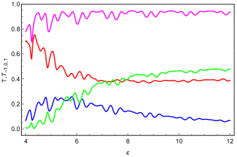
(a)

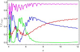
(b)

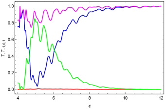
(c)

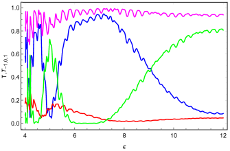
(d)

Figure 2: (Color online) Transmission probabilities as a function of the incident energy $\varepsilon$ for $\omega=1.5$, $k_{y}=1$, $\beta=\frac{\pi}{8}$, $F_{2}=F_{4}=1.5$, and different distances (a): $d_{1}=3$, $d_{2}=5$, (b): $d_{1}=3$, $d_{2}=10$, (c): $d_{1}=1$, $d_{2}=5$, (d): $d_{1}=1$, $d_{2}=10$. With $T_{1}$ (red line), $T_{-1}$ (green line), $T_{0}$ (blue line), and $T$ (magenta line).

Fig. 2 depicts the transmission probability as a function of the incoming energy $\varepsilon$ for various values of $d_{1}$, the spacing between the two barriers, and $d_{2}$, the width of the two barriers. To have a transmission, it is necessary that the following condition: $\varepsilon>k_{y}+2\varpi$ should be fulfilled. As a result, we can say that the quantity $k_{y}+2\varpi$ plays the role of an effective mass [31]. We observe that the transmission varies in an oscillatory way, and the total transmission oscillates in the vicinity of unity. Fig. 2a plotted for $d_{1}=3$ and $d_{2}=5$, we see that the transmission with photon emission $T_{1}$ (red line) decreases exponentially, the transmission with absorption $T_{-1}$ (green line) increases along the $\varepsilon$-axis, and the transmission $T_{0}$ with zero photon exchange (blue line) decreases rapidly towards zero. When the width of the barrier is increased,  $T_{-1}$ becomes null from $\varepsilon=7$ but $T_{1}$ increases, and $T_{0}$ shows different behaviors varying between decreasing then increasing along the $\varepsilon-$axis as depicted in Fig. 2b.  For the particular values $d_{1}=1$ and $d_{2}=10$, $T_{1}$ is almost zero for all incident energies, $T_{-1}$ increases then decreases exponentially, and $T_{0}$ shows the opposite behavior (decreases then increases exponentially). From the energy $E=10$, we notice that the transmission is carried out only with zero photon exchange ($T_{0}$) and then all fermions cross the barrier, showing the Klein tunnel. When the width of the barrier is increased to $d_{2}=10$ in Fig. 2d, we observe that $T_{0}$ is dominant between $\varepsilon=6$ and $\varepsilon=9$, and after that, $T_{1}$ becomes more dominant but $T_{-1}$ is almost null. As a conclusion, varying the two distances makes it possible to control the mode of transmission, meaning that we can vary the mode of transmission by changing the two distances, but the Klein paradox is still present.

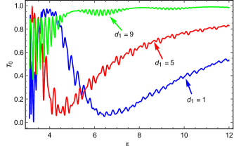
(a)

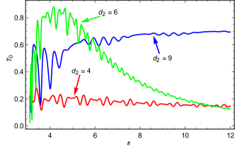
(b)

Figure 3: (Color online) Transmission probability with zero photon exchange $T_{0}$ as a function of $\varepsilon$ for $\beta=0$, $k_{y}=0.1$, $\varpi=1.5$, $F_{2}=F_{4}=1.5$, and different distances ($d_{1},d_{2}$) such that (a): $d_{2}=10$, $d_{1}=1$ (blue line), $d_{1}=5$ (red line), $d_{1}=9$ (green line), and (b): $d_{1}=3$, $d_{2}=4$ (blue line), $d_{1}=6$ (red line), $d_{1}=9$ (green line).

In Fig. 3 we have plotted the transmission of the central band corresponding to $l=0$ as a function of the incident energy of the fermions for different values of $d_{1}$ and $d_{2}$ for well-determined values of other variables. Fig. 3a depicts for various spacing values of $d_{1}$ between the two barriers. We can see that as the distance increases, the transmission process with zero photon exchange $T_{0}$ becomes more dominant because the two barriers become like two peaks of width $d=d_{2}-d_{1}$. In this case, most of the incident fermions cross the barrier with zero photon exchange, as clearly seen in the green curve, which corresponds to $d=9$. Fig. 3b is plotted for different values of the barrier width $d_{2}$, and we notice that for $d_{2}$, which is almost equal to $d_{1}$ (red line), $T_{0}$ is  very weak and decreases in an oscillatory way. For $d_{2}=2d_{1}$ (green line),  $T_{0}$ increases for low energies, then decreases exponentially towards zero in the vicinity of $\varepsilon=11$. For $d_{2}=3d_{1}$ (blue line),  $T_{0}$ becomes more important than the other transmission process because the sum of the three transmission modes is close to unity, as we have seen in the previous figures. We can conclude that increasing the barrier width suppresses the transmission of the side bands and increases the transmission with zero photon exchange.

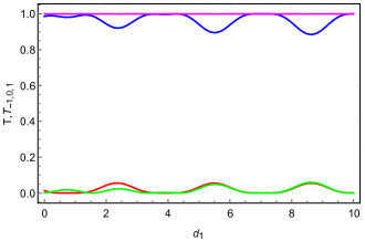
(a)

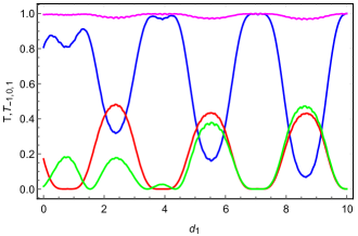
(b)

(c)

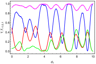
(d)

Figure 4: (Color online) Transmission probabilities as a function of $d_{1}$ for $d_{2}=10$, $k_{y}=1$, $\varpi=2$, $\varepsilon=20$, $\beta=0$, and different amplitudes $F$ ($F_{1}=F_{4}=F$) such that (a): $F=0.5$, (b): $F=1.9$, (c): $F=2.9$, (d): $F=3.9$. With $T$ (magenta line), $T_{0}$ (blue line), $T_{1}$ (red line), $T_{-1}$ (green line).

In Fig. 4, we present the transmission probabilities as a function of the distance between the two barriers $d_{1}$ for different values of the amplitude $F$ of the laser field. Fig. 4a is plotted for $F=0.5$, and we observe that the total transmission $T$ (magenta line) almost equals unit whatever the distance $d_{1}$ because the laser fields are very weak and they have almost a negligible effect. The transmission with zero photon exchange $T_{0}$ oscillates in the vicinity of unit, and the transmissions ($T_{1}$, $T_{-1}$) with photon exchange oscillate in the vicinity of zero. The laser fields are very weak but allow for quantifying the energy, even though the majority of the fermions cross the barrier with zero photon exchange. Fig. 4b is plotted for $F=1.9$, and hence that the laser effect is very clear because we observe that the transmissions with photon exchange vary periodically, showing that  $T_{1}$ (red line) decreases and $T_{-1}$ increases along the $d_{1}$-axis. However, $T_{0}$ varies in phase opposition with the two other transmission modes, with an increase in the amplitude of the oscillations along the $d_{1}$ axis. The total transmission always oscillates in the vicinity of the unit, meaning the Klein effect is present. Now, by increasing to the value $F=2.9$ in Fig. 4c, $T_{0}$ oscillates along the $d_{1}$-axis, and with an increase in the amplitude of the oscillations, it vanishes for very precise values. The intervals at which this transmission is obtained are maximal, and the transmissions with photon exchanges are zero. Fig. 4d is plotted for $F=3.9$, that is to say $\alpha=\frac{F}{\omega^{2}}$ is closed to $1$, we observe a decrease in the interval where $T_{1}$ and $T_{-1}$ get canceled with an increase in the number of peaks. We see that $T_{1}$ oscillates with a decrease in amplitude, and in contrast,  $T_{-1}$ increases along the $d_{1}$-axis. As a result, it appears that increasing the amplitude $F$ of the laser fields makes it possible to decrease the interval of cancellation of the transmissions, but it also increases the number of oscillations.

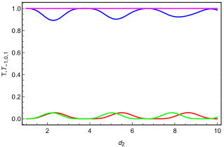
(a)

(b)

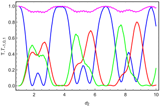
(c)

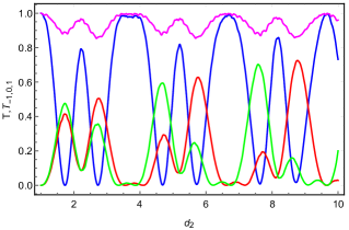
(d)

Figure 5: (Color online) Transmission probabilities as a function of $d_{2}$ for $d_{2}=10$, $k_{y}=1$, $\varpi=2$, $\varepsilon=20$, $\beta=0$, and different amplitudes $F$ ($F_{2}=F_{4}=F$) such that (a): $F=0.5$, (b): $F=1.9$, (c): $F=2.9$, (d): $F=3.9$. With $T$ (magenta line), $T_{0}$ (blue line), $T_{1}$ (red line), $T_{-1}$ (green line).

Fig. 5 is similar to the previous figure with a variation of the barrier widths and the same parameter values. Fig. 5a is plotted for $F=0.5$, and then the generation of transmission modes is observed, but the effect of the laser fields is very weak. The transmissions $T_{1}$ and $T_{-1}$ oscillate around zero, which  can be neglected in comparison to $T_{0}$, implying a very clear Klein effect. For the value $F=1.9$ in Fig. 5b, $T_{1}$ and $T_{-1}$ vary periodically with the increase in amplitude, but  $T_{0}$ varies in an oscillatory way with the decrease in the amplitude  along the $d_{2}$-axis. For $F=2.9$, Fig. 5c shows that $T_{0}$ varies regularly with the appearance of peaks in the minimum part. For $F=3.9$ in Fig. 5d, we observe that the total transmission $T$ oscillates around the unit, while $T_{0}$ is more dominant, which is oscillating between zero and one, canceling out at several points, $T_{1}$ and $T_{-1}$ also oscillate with the increase in amplitude along the $d_{2}$-axis. For example, in the vicinity of the value $d_{2}=4$, $T_{1}$ and $T_{-1}$ almost null, but $T_{0}$ is equal to the unit, which implies that all the fermions cross the barrier without exchanging photons. There are several points where transmissions get canceled. From the width of the barriers, it is possible to control the passage by which transmission mode.

Fig. 6 presents the transmission probabilities as a function of the phase shift $\beta$  for $k_{y}=1$, $\varpi=2$, $\varepsilon=12$, $F_{2}=2$, $d_{1}=1.3$,  $d_{2}=3$, and different values of the amplitude $F_{4}$ of the second laser barrier. For $F_{4}=0.9$ in Fig. 6a, we notice that the three transmission modes vary in an oscillating way with the same frequency for different amplitudes. The transmission with zero photon exchange $T_{0}$ is more dominant, while the transmission with photon emission $T_{1}$ and absorption $T_{-1}$ vary in the same way. A similar result is obtained in [32] for a double oscillating potential. The total transmission $T$ oscillates around the unit, which implies the presence of the Klein effect. Fig. 6b is plotted for $F_{4}=2$ that is to say $\alpha_{1}=\alpha_{2}$, in this case, the amplitude of the oscillations increases, but $T_{0}$ is still more dominant and $T$ is still fluctuating around the unit. In Fig. 6c with $F_{4}=2.9$, we see that the transmissions become non-sinusoidal but vary periodically. $T_{0}$ is always more dominant, and its amplitude is almost equal to $0.9$, whereas $T_{1}$ and $T_{-1}$ vary symmetrically. In addition, we observe that the Klein tunnel presents periodically for very precise values of $\beta$. When $\alpha_{4}$ tends towards $1$, Fig. 6d shows that the amplitude of $T_{0}$ decreases with the increase in the number of oscillations, and the Klein tunnel is exhibited periodically as before.

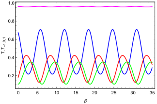
(a)

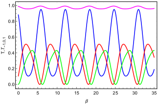
(b)

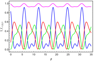
(c)

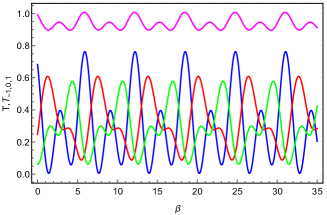
(d)

Figure 6: (Color online) Transmission probabilities as a function of the phase shift $\beta$ for $k_{y}=1$, $\varpi=2$, $\varepsilon=12$, $F_{2}=2$, $d_{1}=1.3$ $d_{2}=3$, and different value of amplitude $F_{4}$ such that (a): $F_{4}=0.9$, (b): $F_{4}=2$, (c): $F_{4}=2.9$, (d): $F_{4}=3.9$. With $T$ (magenta line), $T_{0}$ (blue line), $T_{1}$ (red line), $T_{-1}$ (green line).

IV Conclusion

We have studied the behavior of Dirac fermions through double laser barriers generated by two electric fields, the first of amplitude $F_{2}$ and the second of amplitude $F_{4}$, and of frequency $\omega$ shifted by a phase shift $\beta$. The two barriers divide the graphene sheet into five regions. In regions 1, 3, and 5, there is only pristine graphene, and the other two regions are irradiated by laser fields. Within the framework of Floquet’s approximation, we solved the eigenvalue equation to determine the wave functions corresponding to each region. The oscillation of the barrier over time generates several energy bands. Then, using the boundary conditions of each barrier, we obtained eight equations, each of which has several modes. To simplify the calculation, we used the matrix formalism to arrive at a transfer matrix of infinite order. The latter is difficult to solve, and for this reason we have limited our study to the first three energy bands: the central band corresponds to the energy $\varepsilon$ and the first two side bands correspond to the $\varepsilon+\varpi$. The current densities are also used to determine the transmission coefficient corresponding to each energy band.

The numerical analysis of our theoretical results shows that the transmission exists if the incidence energy of the Dirac fermions satisfy the condition $\varepsilon>k_{y}+2\varpi$, such that this threshold plays the role of an effective mass. The vibration of the barrier over time produces two transmission processes: the transmission process with zero photon exchange and the process with photon exchange. The variation of the distance between the two barriers makes it possible to cancel one of the two processes, and the variation of the width of the barriers makes it possible to change the transmission process. When the distance between the two barriers $d_{1}$ is increased, the number of oscillations increases, and the transmission with zero photon exchange becomes more dominant. The decrease in the width of the barrier $d_{2}$ makes it possible to reduce the transmission $T_{0}$ even if the incident energy increases. The increase in laser field amplitude increases the number of oscillations and their amplitude. The Klein tunnel is observed periodically, and it is obtained for very precise values of the phase shift $\beta$.

Appendix A Determining transmission channels

The continuity of the wave function at the barrier edges makes it possible to find eight equations, each of which has an infinity mode. The analytical resolution of this system is difficult. For simplification, we use the matrix formalism, which allows us to write this system in matrix form with an infinite order transfer matrix. To simplify, we limit our study to the three first bands: the central band corresponds to $l=0$ and the two first side bands correspond to $l=\pm 1$. For the first barrier, we have $\Psi_{1}(-d_{2},y,t)=\Psi_{2}(-d_{2},y,t)$ and $\Psi_{2}(-d_{1},y,t)=\Psi_{3}(-d_{1},y,t)$, which give

$$\delta_{m,0}e^{-ik^{0}_{x}d_{2}}+r_{m}e^{+ik^{m}_{x}d_{2}}=\sum_{l=-\infty}^{+\infty}\left(a_{1l}e^{-iq^{l}_{x}d_{2}}+a_{2l}e^{+iq^{l}_{x}d_{2}}\right)J_{m-l}(\alpha_{2})$$ (44)

$$\delta_{m,0}\gamma_{m}e^{-ik^{0}_{x}d_{2}}-r_{m}\gamma^{*}_{m}e^{+ik^{m}_{x}d_{2}}=\sum_{l=-\infty}^{+\infty}\left(a_{1l}\Gamma_{l}e^{-iq^{l}_{x}d_{2}}-a_{2l}\Gamma^{*}_{l}e^{+iq^{l}_{x}d_{2}}\right)J_{m-l}(\alpha_{2})$$ (45)

$$c_{1m}e^{-ik^{m}_{x}d_{1}}+c_{2m}e^{+ik^{m}_{x}d_{1}}=\sum_{l=-\infty}^{+\infty}\left(a_{1l}e^{-iq^{l}_{x}d_{1}}+a_{2l}e^{+iq^{l}_{x}d_{1}}\right)J_{m-l}(\alpha_{2})$$ (46)

$$c_{1m}\gamma_{m}e^{-ik^{m}_{x}d_{1}}-c_{2m}\gamma^{*}_{m}e^{+ik^{m}_{x}d_{1}}=\sum_{l=-\infty}^{+\infty}\left(a_{1l}\Gamma_{l}e^{-iq^{l}_{x}d_{1}}-a_{2l}\Gamma^{*}_{l}e^{+iq^{l}_{x}d_{1}}\right)J_{m-l}(\alpha_{2}).$$ (47)

For the second barrier we have $\Psi_{3}(d_{1},y,t)=\Psi_{4}(d_{1},y,t)$ and $\Psi_{4}(d_{2},y,t)=\Psi_{5}(d_{2},y,t)$, which give

$$c_{1m}e^{ik^{m}_{x}d_{1}}+c_{2m}e^{-ik^{m}_{x}d_{1}}=\sum_{l=-\infty}^{+\infty}\left(b_{1l}e^{iq^{l}_{x}d_{1}}+b_{2l}e^{-iq^{l}_{x}d_{1}}\right)e^{-i(m-l)\beta}J_{m-l}(\alpha_{4})$$ (48)

$$c_{1m}\gamma_{m}e^{ik^{m}_{x}d_{1}}-c_{2m}\gamma^{*}_{m}e^{-ik^{m}_{x}d_{1}}=\sum_{l=-\infty}^{+\infty}\left(b_{1l}\Gamma_{l}e^{iq^{l}_{x}d_{1}}-b_{2l}\Gamma^{*}_{l}e^{-iq^{l}_{x}d_{1}}\right)e^{-i(m-l)\beta}J_{m-l}(\alpha_{4})$$ (49)

$$t_{m}e^{ik^{m}_{x}d_{2}}+\mathbb{0}_{m}e^{-ik^{m}_{x}d_{2}}=\sum_{l=-\infty}^{+\infty}\left(b_{1l}e^{iq^{l}_{x}d_{2}}+b_{2l}e^{-iq^{l}_{x}d_{2}}\right)e^{-i(m-l)\beta}J_{m-l}(\alpha_{4})$$ (50)

$$t_{m}\gamma_{m}e^{ik^{m}_{x}d_{2}}-\mathbb{0}_{m}\gamma^{*}_{m}e^{-ik^{m}_{x}d_{2}}=\sum_{l=-\infty}^{+\infty}\left(b_{1l}\Gamma_{l}e^{iq^{l}_{x}d_{2}}-b_{2l}\Gamma^{*}_{l}e^{-iq^{l}_{x}d_{2}}\right)e^{-i(m-l)\beta}J_{m-l}(\alpha_{4}).$$ (51)

We can write all sets of equations in matrix form as follows

$$\begin{pmatrix}\delta_{m,0}\\ r_{m}\end{pmatrix}=\begin{pmatrix}\mathbb{S}_{1,1}&\mathbb{S}_{1,2}\\ \mathbb{S}_{2,1}&\mathbb{S}_{2,2}\end{pmatrix}\begin{pmatrix}t_{m}\\ \mathbb{0}_{m}\end{pmatrix}=\mathbb{S}\begin{pmatrix}t_{m}\\ \mathbb{0}_{m}\end{pmatrix}$$ (52)

where $\mathbb{S}$ is the total transfer matrix. The transfer matrix $\mathbb{S}$ has infinite order to simplify we go to finite order, so we take $m$ included between -$N$ and $N$, knowing that $N>\alpha_{j}$ [22], whit $\mathbb{S}$ is the matrix product of the transfer matrix for each region (53), and $\mathbb{S}(j,j+1)$ the transfer matrix of the region $j$ to region $j+1$

$$\mathbb{S}=\mathbb{S}(1,2).\mathbb{S}(2,3).\mathbb{S}(3,4).\mathbb{S}(4,5)$$ (53)

with

$$\mathbb{S}(1,2) = \begin{pmatrix}\mathbb{G}^{0}_{-d_{2}}&\mathbb{G}_{d_{2}}\\ \mathbb{R}_{+,-d_{2}}^{+1}&\mathbb{R}_{-,d_{2}}^{-1}\\ \end{pmatrix}^{-1}\begin{pmatrix}\mathbb{H}_{+,-d_{2}}^{2}&\mathbb{H}_{+,d_{2}}^{2}\\ \mathbb{L}_{+,-d_{2}}^{2,+1}&\mathbb{L}_{-,d_{2}}^{2,-1}\\ \end{pmatrix}$$ (54)

$$\mathbb{S}(2,3) = \begin{pmatrix}\mathbb{H}_{+,-d_{1}}^{2}&\mathbb{H}_{+,d_{1}}^{2}\\ \mathbb{L}_{+,-d_{1}}^{2,+1}&\mathbb{L}_{-,d_{1}}^{2,-1}\end{pmatrix}^{-1}\begin{pmatrix}\mathbb{G}_{-d_{1}}&\mathbb{G}_{d_{1}}\\ \mathbb{R}_{+,-d_{1}}^{l,+1}&\mathbb{R}_{-,d_{1}}^{l,-1}\\ \end{pmatrix}$$ (55)

$$\mathbb{S}(3,4) = \begin{pmatrix}\mathbb{G}_{d_{1}}&\mathbb{G}_{-d_{1}}\\ \mathbb{R}_{+,d_{1}}^{+1}&\mathbb{R}_{-,-d_{1}}^{-1}\\ \end{pmatrix}^{-1}\begin{pmatrix}\mathbb{K}^{4}_{+,-d_{1}}&\mathbb{K}^{4}_{+,d_{1}}\\ \mathbb{F}^{4,+}_{+,d_{1}}&\mathbb{F}^{4,+}_{-,-d_{1}}\\ \end{pmatrix}$$ (56)

$$\mathbb{S}(4,5) = \begin{pmatrix}\mathbb{K}^{4}_{+,d_{2}}&\mathbb{K}^{4}_{+,-d_{2}}\\ \mathbb{F}^{4,+}_{+,d_{2}}&\mathbb{F}^{4,+}_{-,-d_{2}}\\ \end{pmatrix}^{-1}\begin{pmatrix}\mathbb{G}_{d_{2}}&\mathbb{G}_{-d_{2}}\\ \mathbb{R}_{+,d_{2}}^{+1}&\mathbb{R}_{-,-d_{2}}^{-1}\\ \end{pmatrix}$$ (57)

where $z=\pm d_{1,2}$ and we have set

$$(\mathbb{G}^{0}_{z})=e^{ik^{0}_{x}z}$$ (58)

$$(\mathbb{G}_{z})_{m,l}=e^{ik^{l}_{x}z}\delta_{m,l}$$ (59)

$$(\mathbb{R}_{\pm,z}^{\pm 1})_{m,l}=\pm\gamma_{l}^{\pm 1}e^{ik^{l}_{x}z}\delta_{m,l}$$ (60)

$$(\mathbb{H}^{j}_{\pm,z})_{m,l}=\pm e^{iq^{l}_{x}z}J_{m-l}(\alpha_{j})$$ (61)

$$(\mathbb{L}_{\pm,z}^{j,\pm 1})_{m,l}=\pm\Gamma_{l}^{\pm 1}e^{iq^{l}_{x}z}J_{m-l}(\alpha_{j})$$ (62)

$$(\mathbb{K}^{j}_{\pm,z})_{m,l}=\pm e^{iq^{l}_{x}z}J_{m-l}(\alpha_{j})e^{-i(m-l)\beta}$$ (63)

$$(\mathbb{F}_{\pm,z}^{j,\pm 1})_{m,l}=\pm\Gamma_{l}^{\pm 1}e^{iq^{l}_{z}}J_{m-l}(\alpha_{j})e^{-i(m-l)\beta}.$$ (64)

We assume the electron propagation direction is from left to right with energy $\varepsilon$, therefore, the transmission coefficient of the m-$th$ band is written as follows:

$$t_{m}=\mathbb{S^{\prime}}\delta_{m,0}$$ (65)

with $\mathbb{S^{\prime}}=\mathbb{S}^{-1}_{1,1}$. Recall that $m$ varies from -$N$ to $N$, that is to say

$$\begin{pmatrix}t_{-N}\\ .\\ .\\ t_{-1}\\ t_{0}\\ t_{1}\\ .\\ .\\ t_{N}\end{pmatrix}=\mathbb{S^{\prime}}\begin{pmatrix}0\\ .\\ .\\ 0\\ 1\\ 0\\ .\\ .\\ 0\end{pmatrix}.$$ (66)

To simplify, we have limited our study to the three first bands: the central band corresponding to the energy $E$ and the two first side bands corresponding to the energy $\varepsilon\pm\varpi$. In this case, we obtain

$$t_{-1}=\mathbb{S^{\prime}}[1,2]$$ (67)

$$t_{0}=\mathbb{S^{\prime}}[2,2]$$ (68)

$$t_{1}=\mathbb{S^{\prime}}[3,2].$$ (69)

On the other hand, the transmission probability can be obtained from the electric current density, which is also found using the continuous equation $J=\Psi^{\dagger}\sigma_{x}\Psi$. Thus, the different current densities are given as follows:

$$J^{0}_{\text{inc}}=\gamma_{0}+\gamma^{*}_{0}$$ (70)

$$J^{m}_{\text{ref}}=r_{m}r_{m}^{*}(\Gamma_{m}+\Gamma^{*}_{m})$$ (71)

$$J^{m}_{\text{tra}}=t_{m}t_{m}^{*}(\gamma_{m}+\gamma^{*}_{m})$$ (72)

where $\gamma_{m}=s_{m}\frac{k^{m}_{x}+i(k_{y}-m\omega)}{\sqrt{(k^{m}_{x})^{2}+(k_{y}-\varpi)^{2}}}$ and $\Gamma_{m}=s_{m}\frac{q^{m}_{x}+i(k_{y}-m\omega)}{\sqrt{(q^{m}_{x})^{2}+(k_{y}-m\varpi)^{2}}}$. The transmission corresponds to the $m$-th side-band, is given by the following relation

$$T_{m}=\frac{\cos\theta_{m}}{\cos\theta_{0}}|t_{m}|^{2}$$ (73)

where $\cos\theta_{m}=\frac{k_{x}^{m}}{\sqrt{(k_{x}^{m})^{2}+k_{y}^{2}}}$ and $k_{x}^{m}=\sqrt{(\varepsilon+m\varpi)^{2}-k_{y}^{2}}$. Finally, the total transmission probability is given by the sum over all modes

$$T=\sum_{m=-N}^{N}T_{m}.$$ (74)

References

- [1] A. K. Geim and K. S. Novoselov, Nat. Mater. 6, 183 (2007).
- [2] K. S. Novoselov, A. K. Geim, S. V. Morozov, D. Jiang, M. I. Katsnelson, I. V. Grigorieva, S. V. Dubonos, and A. A. Firsov, Nature 438, 197 (2005).
- [3] K. S. Novoselov, A. K. Geim, S. V. Morozov, D. Jiang, Y. Zhang, S. V. Dubonos, I. V. Grigorieva, and A. A. Firsov, Science 306, 666 (2004).
- [4] A. H. Castro Neto, F. Guinea, N. M. R. Peres, K. S. Novoselov, and A. K. Geim, Rev. Mod. Phys. 81, 109 (2009).
- [5] Y. Zhang, Y. W. Tan, H. L. Stormer, and P. Kim, Nature 438, 201 (2005).
- [6] S. Morozov, K. Novoselov, M. Katsnelson, F. Schedin, D. Elias, J. Jaszczak, and A. Geim, Phys. Rev. Lett. 100, 016602 (2008).
- [7] K. I. Bolotin, K. J. Sikes, Z. Jiang, M. Klima, G. Fudenberg, J. Hone, P. Kim, and H. L. Stormer, Solid State Commun. 351. 146 (2008).
- [8] A. K. Geim, Science 324, 1530 (2009).
- [9] Qiaoliang Bao, Han Zhang, Bing Wang, Zhenhua Ni, Candy Haley Yi Xuan Lim, Yu Wang, Ding Yuan Tang, and Kian Ping Loh, Nature Photon 5, 411 (2011).
- [10] S. Reich, J. Maultzsch, C. Thomsen, and P. Ordejon, Phys. Rev. B 66, 035412 (2002).
- [11] N. M. R. Peres, J. Phys.: Condens. Matter 21, 323201 (2009).
- [12] M. I. Katsnelson, K. S. Novoselov, and A. K. Geim, Nat. Phys. 2, 620 (2006).
- [13] C. W. J. Beenakker, Rev. Mod. Phys. 80, 1337 (2008).
- [14] N. Stander, B. Huard, and D. Goldhaber-Gordon, Phys. Rev. Lett. 102, 026807 (2009).
- [15] A. N. Sidorov, M. M. Yazdanpanah, R. Jalilian, P. J. Ouseph, R. W. Cohn, and G. U. Sumanasekera, Nanotechnology 18, 135301 (2007).
- [16] G. A. K. P. A. Giovannetti, P. A. Khomyakov, G. Brocks, V. V. Karpan, J. van den Brink, and P. J. Kelly, Phys. Rev. Lett. 101, 026803 (2008).
- [17] F. Guinea, M. I. Katsnelson, and A. K. Geim, Nat. Phys. 6, 30 (2010).
- [18] G.-X. Ni, Y. Zheng, S. Bae, H. R. Kim, A. Pachoud, Y. S. Kim, C.-L. Tan, D. Im, J.-H. Ahn, B. H. Hong, and B. Ozyilmaz, ACS Nano 6, 1158 (2012).
- [19] H. Bahlouli, E. B. Choubabi, A. El Mouhafid, and A. Jellal, Solid State Communi. 151, 1309 (2011).
- [20] L. Dell’Anna and A. De Martino, Phys. Rev. B 79, 045420 (2009).
- [21] A. Jellal and A. El Mouhafid, J. Phys. A: Math. Theo. 44, 015302 (2011).
- [22] A. Jellal, M. Mekkaoui, E. B. Choubabi, and H. Bahlouli, Eur. Phys. J. B 87, 123 (2014).
- [23] M. Ahsan Zeb, K. Sabeeh, and M. Tahir, Phys. Rev. B 78, 165420 (2008).
- [24] A. El Mouhafid and A. Jellal, J. Low Temp. Phys. 173, 264 (2013).
- [25] R. El Aitouni, M. Mekkaoui, A. Jellal, and M. Schreiber, arXiv:2307.03999 (2023).
- [26] R. Biswas, S. Maitty, and C. Sinha, Physica E 84, 235 (2016).
- [27] R. Biswas and C. Sinha, Appl. Phys. 114, 183706 (2013).
- [28] R. El Aitouni, M. Mekkaoui, and A. Jellal, Ann. Phys. (Berlin) 535, 2200630 (2023).
- [29] R. El Aitouni and A. Jellal, Phys. Lett. A. 447, 128288 (2022).
- [30] C. W. J. Beenakker, Rev. Mod. Phys, 80, 1337 (2008).
- [31] M. Mekkaoui, A. Jellal, and H. Bahlouli, Solid State Communi. 358, 114981 (2022).
- [32] M. Mekkaoui, E. B. Choubabi, A. Jellal, and H. Bahlouli, Mater. Res. Express 4, 035002 (2017).