On the generalized dimensions of chaotic attractors

Abstract

We prove that if $\mu$ is the physical measure of a chaotic flow diffeomorphically conjugated to a suspension flow based on a Poincaré application $R$ with physical measure $\mu_{R}$, $D_{q}(\mu)=D_{q}(\mu_{R})+1$, where $D_{q}$ denotes the generalized dimension of order $q$ with $q\neq 1$. We also prove that a similar result holds for the local dimensions so that, under the additional hypothesis of exact-dimensionality of $\mu_{R}$, our result extends to the case $q=1$. We then apply these results to estimate the $D_{q}$ spectrum of the Rössler attractor and prove the existence of the information dimension $D_{1}$ for the Lorenz ’63 flow.

AMS subject classification:

37C10, 37D45, 37E05

Keywords and phrases:

generalized dimensions, chaotic attractor, Rössler flow, Lorenz-like flows.

1 Introduction

Generalized dimensions have been introduced in 1983 by Hentschel and Procaccia to describe the variety of different scaling behaviors of physical measures of chaotic dynamical systems [HP]. This spectrum of dimensions plays a central role in the synchronization properties of chaotic dynamical systems [CF, RT, BR], as well as in the distributions of local quantities of interest, such as local dimensions and recurrence times [CF]. Let us now recall the definition of these objects and that of some related notions.

Definition 1

Let $\nu$ be a probability measure on $\left(\mathbb{R}^{d},\mathcal{B}\left(\mathbb{R}^{d}\right)\right),d\geq 1$ and, for any $x\in\mathbb{R}^{d},$ let $B_{r}^{\left(d\right)}\left(x\right):=\left\{y\in\mathbb{R}^{d}:\left|x-y\right|\leq r\right\}$ be the Euclidean ball of radius $r$ centered in $x.$

1. The generalized dimension of order $q$ of $\nu$ is given by

   $$D_{q}\left(\nu\right):=\left\{\begin{array}[c]{cc}\frac{1}{q-1}\lim_{r\downarrow 0}\frac{\log\int\nu\left(dx\right)\nu^{q-1}\left(B_{r}^{\left(d\right)}\left(x\right)\right)}{\log r}&\text{if }q\neq 1\\ \lim_{r\downarrow 0}\frac{\int\nu\left(dx\right)\log\nu\left(B_{r}^{\left(d\right)}\left(x\right)\right)}{\log r}&\text{if }q=1\end{array}\right.$$ (1)

   provided the limit exists.

2. The local dimension at $x\in\mathbb{R}^{d}$ is defined as

   $$d_{\nu}(x):=\lim_{r\downarrow 0}\frac{\log\nu(B_{r}^{(d)}(x))}{\log r}\,$$ (2)

   provided the limit exists.

3. We say that $\nu$ is exact-dimensional if $d_{\nu}(\cdot)$ is well defined and constant $\nu$-almost everywhere (in which case this typical value is $D_{1}(\nu)$).

Generalized dimensions and local dimensions are closely related within the so-called multifractal formalism, which has been developed along the years in analogy with thermodynamics [Pe]. The $D_{q}$ spectrum provides a comprehensive description of the geometric structure of the measure, including the information dimension $(q=1)$, the correlation dimension $(q=2)$, and the box-counting dimension of the support of the measure $(q=0)$. In different recent publications, it is used to gauge the convergence of the geometric structure of the physical measures of coupled chaotic systems, in a process that was termed topological synchronization [L1, L2].
Although many efforts have been put forward to numerically estimate these quantities, the designed algorithms are known to be subject to important numerical errors, especially for negative $q$ [PSR]. For flows, this adds up to the accumulated errors associated with the discretization process, yielding unreliable estimates.
In this paper, we will study in detail the $D_{q}$ spectrum associated with physical measures of chaotic flows in $\mathbb{R}^{d}$, $d\geq 3$, that are diffeomorphically to a suspension flows. To be more specific, let $\Sigma$ be a compact $\left(d-1\right)$-dimensional manifold that stands for a Poincaré surface and $R:\Sigma\circlearrowleft$ a return map with physical measure $\mu_{R}$. We denote $\mathfrak{t}$ the associated roof function and suppose $\mathfrak{t}\in L^{1}(\mu_{R})$. Note that $\mathfrak{t}$ is a $C^{1}\left(\Sigma,\mathbb{R}_{+}\right)$ function provided the velocity field is at least $C^{1}$. Setting $\mathfrak{s}_{0}:=0,\mathfrak{s}_{1}:=\mathfrak{t}$ and $\forall n\geq 2,$

$$\Sigma\ni\xi\longmapsto\mathfrak{s}_{n}\left(\xi\right):=\sum_{k=1}^{n}\mathfrak{t\circ}R^{k}\in\mathbb{R}_{+}\ ,$$ (3)

$\forall\xi\in\Sigma$ we denote by

$$\mathfrak{n}\left(\xi,t\right):=\max\left\{n\in\mathbb{N}:\mathfrak{s}_{n}\left(\xi\right)\leq t\right\}$$ (4)

and by

$$\Sigma_{\mathfrak{t}}:=\left\{\left(\xi,t\right)\in\Sigma\times\mathbb{R}_{+}:t\in\left[0,\mathfrak{t}\left(\xi\right)\right]\right\}\ .$$ (5)

We then define the suspension semi-flow $\left(S^{t},\ t\geq 0\right)$

$$\Sigma_{\mathfrak{t}}\ni\left(\xi,s\right)\longmapsto S^{t}\left(\xi,s\right):=\left(R^{\mathfrak{n}\left(\xi,t+s\right)}\left(\xi\right),t+s-\mathfrak{s}_{\mathfrak{n}\left(\xi,t+s\right)}\right)\in\Sigma_{t}\ ,\;t\geq 0$$ (6)

whose physical measure $\mu_{S}$ has density $\frac{\mathbf{1}_{\left[0,\mathfrak{t}\right]}}{\mu_{R}\left[\mathfrak{t}\right]}$ w.r.t. $\mu_{R}\otimes\lambda,$ where $\lambda$ is the Lebesgue measure on $\left(\mathbb{R},\mathcal{B}\left(\mathbb{R}\right)\right).$ We define

$$\Sigma_{\mathfrak{t}} \ni\left(\xi,t\right)\longmapsto\pi_{1}\left(\xi,t\right):=t\in\mathbb{R}_{+}\ ,$$ (7)

$$\Sigma_{\mathfrak{t}} \ni\left(\xi,t\right)\longmapsto\pi_{2}\left(\xi,t\right):=\xi\in\Sigma\ .$$ (8)

We suppose that there exists a diffeomorphism $\Theta$ mapping $\mathring{\Sigma}_{\mathfrak{t}}$ to an open set $\mathcal{U}\subset\mathbb{R}^{d}$ and a semi-flow $\left(\chi^{t},t\geq 0\right)$ in $\mathbb{R}^{d}$ such that $\forall t\geq 0,\Theta\circ S^{t}=\chi^{t}\circ\Theta.$ The physical measure $\mu$ of $\left(\chi^{t},t\geq 0\right)$ is then the push-forward under $\Theta$ of $\mu_{S}$.
The above construction is a standard one and applies to well-studied chaotic flows, such as the Rössler and the Lorenz ’63 one.
We start by stating our main general results, which relate $D_{q}(\mu)$ to $D_{q}(\mu_{R})$ for such flows. Parts of the technical details of the proof will be performed in the appendix.
We then apply these results to show that the estimates of the Generalized dimensions of the Rössler attractor should be somehow trivial. Indeed, the strong contraction of the flow along the $z$ axis renders the intersection of the attractor with a suitable Poincaré section indistinguishable, up to machine precision, from a uni-dimensional curve. As a consequence, the geometric structure of the numerically created attractor relates to that of a uni-dimensional return map, which turns out to belong to the family of S-unimodal maps. The characteristics of such maps have been widely studied in the literature and their physical measures are well-known. This will allow us to give an explicit formula for their $D_{q}$ spectrum.
Finally, we discuss the case of the classical Lorenz system and show that its information dimension $D_{1}$ is well-defined and can be derived from that of its 2-dimensional base map.

2 Main result

The following theorem contains our main theoretical results relating the fractal dimensions of a flow to those of its base map.

Theorem 2

Suppose $\nu$ is the physical measure of a $C^{1}$ flow in $\mathbb{R}^{d}$ constructed as in the previous section. Then, provided the different dimensions associated with $\mu_{R}$ exist, we have

1. For all $q\neq 1$,

   $$D_{q}\left(\mu\right)=D_{q}\left(\mu_{R}\right)+1\ .$$ (9)

2. For all $x\in\mathcal{U}$,

   $$d_{\mu}(x)=d_{\mu_{R}}(\xi)+1,$$ (10)

   where $\xi=\pi_{2}\circ\Theta^{-1}(x).$

3. If $\mu_{R}$ is exact-dimensional, then

   $$D_{1}(\mu)=D_{1}(\mu_{R})+1.$$ (11)

2.1 Proof of point 1.

1. turns out to be a corollary of the case when the roof function $\mathfrak{t}$ is assumed to be bounded from above. Therefore we will first discuss this case in the following proposition.

Proposition 3

Assume that $\kappa\leq\mathfrak{t}\leq\kappa^{-1}$ for some $\kappa>0.$ for all $q\neq 1$, if $D_{q}\left(\mu_{R}\right)$ is well defined, then

$$D_{q}\left(\mu\right)=D_{q}\left(\mu_{R}\right)+1\ .$$ (12)

The proof of the previous proposition is deferred to the appendix.
In the case when $\mathfrak{t}$ is unbounded, first notice that, for any bounded measurable function $\varphi$ on $\Sigma$ and any $K>0,$

$$\mu_{R}\left[\mathfrak{t}\varphi\right] =\mu_{R}\left[\mathfrak{t}\left(\mathbf{1}_{\left[0,K\right]}\left(\mathfrak{t}\right)+\mathbf{1}_{\left(K,\infty\right)}\left(\mathfrak{t}\right)\right)\varphi\right]$$ (13)

$$=\mu_{R}\left[\left(\mathfrak{t}\wedge K\right)\varphi\right]+\mu_{R}\left[\left(\mathfrak{t}-K\right)\mathbf{1}_{\left(K,\infty\right)}\left(\mathfrak{t}\right)\varphi\right]$$

and

$$\left|\mu_{R}\left[\left(\mathfrak{t}-K\right)\mathbf{1}_{\left(K,\infty\right)}\left(\mathfrak{t}\right)\varphi\right]\right| \leq\mu_{R}\left[\left(\mathfrak{t}-K\right)\mathbf{1}_{\left(K,\infty\right)}\left(\mathfrak{t}\right)\left|\varphi\right|\right]$$ (14)

$$\leq\left\|\varphi\right\|_{\infty}\int_{K}^{\infty}dt\mu_{R}\left\{\mathfrak{t}>t\right\}\ .$$

For any $\varepsilon>0,$ let $K_{\varepsilon}>0$ be such that $\int_{K_{\varepsilon}}^{\infty}dt\mu_{R}\left\{\mathfrak{t}>t\right\}\leq\varepsilon.$ Then, $\forall K>K_{\varepsilon},\xi\in\Sigma,$

$$\mu_{R}\left[\mathfrak{t}\mathbf{1}_{B_{r}^{\left(d-1\right)}\left(\xi\right)}\right] \leq\mu_{R}\left[\left(\mathfrak{t}\wedge K\right)\mathbf{1}_{B_{r}^{\left(d-1\right)}\left(\xi\right)}\right]+\varepsilon$$ (15)

$$\leq K\mu_{R}\left[\mathbf{1}_{B_{r}^{\left(d-1\right)}\left(\xi\right)}\right]+\varepsilon\ .$$

Moreover, if $\varphi>0,$ from (13) we get that $\mu_{R}\left[\mathfrak{t}\varphi\right]\geq\mu_{R}\left[\left(\mathfrak{t}\wedge K\right)\varphi\right].$ Point 1) follows immediately from Proposition 3 and the following lemmata 4 and 5.

Lemma 4

Let $\mu_{R}\left[\mathfrak{t}\right]<\infty.$ Then, for $q>1,D_{q}\left(\nu_{R}\right)=D_{q}\left(\mu_{R}\right).$

Proof. Let us set

$$\nu_{R}^{K}\left(d\xi\right):=\frac{\mu_{R}\left(d\xi\right)\left(\mathfrak{t}\left(\xi\right)\wedge K\right)}{\mu_{R}\left[\mathfrak{t}\wedge K\right]}\ .$$ (16)

Hence, for $q>1,$

$$\int_{\Sigma}\nu_{R}\left(d\xi\right)\nu_{R}^{q-1}\left(B_{r}^{\left(d-1\right)}\left(\xi\right)\right) =\frac{1}{\mu_{R}^{q}\left[\emph{t}\right]}\int_{\Sigma}\mu_{R}\left(d\xi\right)\mathfrak{t}\left(\xi\right)\mu_{R}^{q-1}\left[\mathfrak{t}\mathbf{1}_{B_{r}^{\left(d-1\right)}\left(\xi\right)}\right]$$ (17)

$$\geq\frac{\mu_{R}^{q}\left[\mathfrak{t}\wedge K\right]}{\mu_{R}^{q}\left[\mathfrak{t}\right]}\frac{\int_{\Sigma}\mu_{R}\left(d\xi\right)\left(\mathfrak{t}\left(\xi\right)\wedge K\right)\mu_{R}^{q-1}\left[\mathfrak{t}\mathbf{1}_{B_{r}^{\left(d-1\right)}\left(\xi\right)}\right]}{\mu_{R}^{q}\left[\mathfrak{t}\wedge K\right]}$$

$$\geq\frac{\mu_{R}^{q}\left[\mathfrak{t}\wedge K\right]}{\mu_{R}^{q}\left[\mathfrak{t}\right]}\frac{\int_{\Sigma}\mu_{R}\left(d\xi\right)\left(\mathfrak{t}\left(\xi\right)\wedge K\right)\mu_{R}^{q-1}\left[\left(\mathfrak{t}\wedge K\right)\mathbf{1}_{B_{r}^{\left(d-1\right)}\left(\xi\right)}\right]}{\mu_{R}^{q}\left[\mathfrak{t}\wedge K\right]}$$

$$=\frac{\mu_{R}^{q}\left[\mathfrak{t}\wedge K\right]}{\mu_{R}^{q}\left[\mathfrak{t}\right]}\int_{\Sigma}\nu_{R}^{K}\left(d\xi\right)\left(\nu_{R}^{K}\left(B_{r}^{\left(d-1\right)}\left(\xi\right)\right)\right)^{q-1}\ .$$

On the other hand, for any $\varepsilon>0,$

$$\int_{\Sigma}\mu_{R}\left(d\xi\right)\mathfrak{t}\left(\xi\right)\nu_{R}^{q-1}\left[\mathbf{1}_{B_{r}^{\left(d-1\right)}\left(\xi\right)}\right]\leq\int_{\Sigma}\mu_{R}\left(d\xi\right)\left[\left(\mathfrak{t}\left(\xi\right)\wedge K\right)\nu_{R}^{q-1}\left[\mathbf{1}_{B_{r}^{\left(d-1\right)}\left(\xi\right)}\right]\right]+\varepsilon\ ,$$ (18)

so that,

$$\int_{\Sigma}\nu_{R}\left(d\xi\right)\nu_{R}^{q-1}\left(B_{r}^{\left(d-1\right)}\left(\xi\right)\right) \leq\frac{1}{\left(\mu_{R}\left[\mathfrak{t}\wedge K\right]\right)^{q}}\left\{\int_{\Sigma}\mu_{R}\left(d\xi\right)\left[\left(\mathfrak{t}\left(\xi\right)\wedge K\right)\mu_{R}^{q-1}\left[\mathfrak{t}\mathbf{1}_{B_{r}^{\left(d-1\right)}\left(\xi\right)}\right]\right]+\varepsilon\right\}$$ (19)

$$\leq\frac{\int_{\Sigma}\mu_{R}\left(d\xi\right)\left[\left(\mathfrak{t}\left(\xi\right)\wedge K\right)\left(\mu_{R}\left[\left(\mathfrak{t}\wedge K\right)\mathbf{1}_{B_{r}^{\left(d-1\right)}\left(\xi\right)}\right]+\varepsilon\right)^{q-1}\right]+\varepsilon}{\left(\mu_{R}\left[\mathfrak{t}\wedge K\right]\right)^{q}}\ .$$

Let $q\in(1,2].$ Since, for $a$ and $b>0,\left(a+b\right)^{q-1}\leq a^{q-1}+b^{q-1},$ we have

$$\int_{\Sigma}\nu_{R}\left(d\xi\right)\nu_{R}^{q-1}\left(B_{r}^{\left(d-1\right)}\left(\xi\right)\right) \leq\int_{\Sigma}\nu_{R}^{K}\left(d\xi\right)\left(\nu_{R}^{K}\left(B_{r}^{\left(d-1\right)}\left(\xi\right)\right)\right)^{q-1}+$$ (20)

$$+\left(\frac{\varepsilon}{\mu_{R}\left[\mathfrak{t}\wedge K\right]}\right)^{q-1}+\frac{\varepsilon}{\mu_{R}^{q}\left[\mathfrak{t}\wedge K\right]}$$

$$\leq\int_{\Sigma}\nu_{R}^{K}\left(d\xi\right)\left(\nu_{R}^{K}\left(B_{r}^{\left(d-1\right)}\left(\xi\right)\right)\right)^{q-1}+$$

$$+\varepsilon^{q-1}\left(\frac{K+\varepsilon^{2-q}}{\mu_{R}^{q}\left[\mathfrak{t}\wedge K\right]}\right)\ .$$

For $q>2,$ since

$$\left(\mu_{R}\left[\left(\mathfrak{t}\wedge K\right)\mathbf{1}_{B_{r}^{\left(d-1\right)}\left(\xi\right)}\right]+\varepsilon\right)^{q-1} =\mu_{R}^{q-1}\left[\left(\mathfrak{t}\wedge K\right)\mathbf{1}_{B_{r}^{\left(d-1\right)}\left(\xi\right)}\right]+$$ (21)

$$+\varepsilon\left(q-1\right)\int_{0}^{1}ds\left(\mu_{R}\left[\left(\mathfrak{t}\wedge K\right)\mathbf{1}_{B_{r}^{\left(d-1\right)}\left(\xi\right)}\right]+s\varepsilon\right)^{q-2}$$

$$\leq\mu_{R}^{q-1}\left[\left(\mathfrak{t}\wedge K\right)\mathbf{1}_{B_{r}^{\left(d-1\right)}\left(\xi\right)}\right]+\varepsilon\left(q-1\right)\left(K+\varepsilon\right)^{q-2}\ ,$$

from (19) we get

$$\int_{\Sigma}\nu_{R}\left(d\xi\right)\nu_{R}^{q-1}\left(B_{r}^{\left(d-1\right)}\left(\xi\right)\right) \leq\int_{\Sigma}\nu_{R}^{K}\left(d\xi\right)\left(\nu_{R}^{K}\left(B_{r}^{\left(d-1\right)}\left(\xi\right)\right)\right)^{q-1}+$$ (22)

$$+\varepsilon\frac{\left(q-1\right)\mu_{R}\left[\mathfrak{t}\wedge K\right]\left(K+\varepsilon\right)^{q-2}+1}{\mu_{R}^{q}\left[\mathfrak{t}\wedge K\right]}\ .$$

Then, setting

$$c_{q}\left(K,\varepsilon\right):=\frac{\left(q-1\right)\mu_{R}\left[\mathfrak{t}\wedge K\right]\left(K+\varepsilon\right)^{q-2}+1}{\mu_{R}^{q}\left[\mathfrak{t}\wedge K\right]}\vee\frac{K+\varepsilon^{2-q}}{\mu_{R}^{q}\left[\mathfrak{t}\wedge K\right]}\ ,$$ (23)

we have, for $r<1$

$$\frac{\log\int_{\Sigma}\nu_{R}\left(d\xi\right)\nu_{R}^{q-1}\left(B_{r}^{\left(d-1\right)}\left(\xi\right)\right)}{\log r}\leq\frac{\log\int_{\Sigma}\nu_{R}^{K}\left(d\xi\right)\left(\nu_{R}^{K}\left(B_{r}^{\left(d-1\right)}\left(\xi\right)\right)\right)^{q-1}}{\log r}+$$ (24)

$$+\varepsilon^{\left(q-1\right)\wedge 1}c_{q}\left(K,\varepsilon\right)\frac{\int_{0}^{1}ds\frac{1}{\int_{\Sigma}\nu_{R}^{K}\left(d\xi\right)\left(\nu_{R}^{K}\left(B_{r}^{\left(d-1\right)}\left(\xi\right)\right)\right)^{q-1}+sc_{q}\left(K,\varepsilon\right)\varepsilon^{\left(q-1\right)\wedge 1}}}{\log r}$$

and by (17)

$$\frac{\log\int_{\Sigma}\nu_{R}\left(d\xi\right)\nu_{R}^{q-1}\left(B_{r}^{\left(d-1\right)}\left(\xi\right)\right)}{\log r}\geq\frac{\log\int_{\Sigma}\nu_{R}^{K}\left(d\xi\right)\left(\nu_{R}^{K}\left(B_{r}^{\left(d-1\right)}\left(\xi\right)\right)\right)^{q-1}}{\log r}\ ,$$ (25)

so that the result follows by taking the limit as $r\downarrow 0$ in view of Proposition 3.   

Lemma 5

Let $\mu_{R}\left[\mathfrak{t}\right]<\infty.$ Then, for $q<1,D_{q}\left(\nu_{R}\right)=D_{q}\left(\mu_{R}\right).$

Proof. If $q<1,$ for any $\varepsilon>0,$

$$\int_{\Sigma}\nu_{R}\left(d\xi\right)\frac{1}{\nu_{R}^{1-q}\left(B_{r}^{\left(d-1\right)}\left(\xi\right)\right)}=\frac{1}{\mu_{R}^{q}\left[\mathfrak{t}\right]}\int_{\Sigma}\mu_{R}\left(d\xi\right)\frac{\mathfrak{t}\left(\xi\right)}{\left(\mu_{R}\left[\mathfrak{t}\mathbf{1}_{B_{r}^{\left(d-1\right)}\left(\xi\right)}\right]\right)^{1-q}}$$ (26)

$$\geq\left(\frac{\mu_{R}\left[\mathfrak{t}\wedge K\right]}{\mu_{R}\left[\mathfrak{t}\right]}\right)^{q}\frac{1}{\mu_{R}^{q}\left[\mathfrak{t}\wedge K\right]}\int_{\Sigma}\mu_{R}\left(d\xi\right)\frac{\mathfrak{t}\left(\xi\right)}{\left(\mu_{R}\left[\left(\mathfrak{t}\wedge K\right)\mathbf{1}_{B_{r}^{\left(d-1\right)}\left(\xi\right)}\right]+\varepsilon\right)^{1-q}}$$

$$\geq\left(\frac{\mu_{R}\left[\mathfrak{t}\wedge K\right]}{\mu_{R}\left[\mathfrak{t}\right]}\right)^{q}\frac{1}{\mu_{R}^{q}\left[\mathfrak{t}\wedge K\right]}\int_{\Sigma}\mu_{R}\left(d\xi\right)\frac{\mathfrak{t}\left(\xi\right)\wedge K}{\left(\mu_{R}\left[\left(\mathfrak{t}\wedge K\right)\mathbf{1}_{B_{r}^{\left(d-1\right)}\left(\xi\right)}\right]+\varepsilon\right)^{1-q}}$$

$$\geq\left(\frac{\mu_{R}\left[\mathfrak{t}\wedge K\right]}{\mu_{R}\left[\mathfrak{t}\right]}\right)^{q}\frac{1}{\mu_{R}^{q}\left[\mathfrak{t}\wedge K\right]}\int_{\Sigma}\mu_{R}\left(d\xi\right)\frac{\mathfrak{t}\left(\xi\right)\wedge K}{\mu_{R}^{1-q}\left[\left(\mathfrak{t}\wedge K\right)\mathbf{1}_{B_{r}^{\left(d-1\right)}\left(\xi\right)}\right]}\times$$

$$\times\left(\frac{\mu_{R}\left[\left(\mathfrak{t}\wedge K\right)\mathbf{1}_{B_{r}^{\left(d-1\right)}\left(\xi\right)}\right]}{\mu_{R}\left[\left(\mathfrak{t}\wedge K\right)\mathbf{1}_{B_{r}^{\left(d-1\right)}\left(\xi\right)}\right]+\varepsilon}\right)^{1-q}$$

$$=\left(\frac{\mu_{R}\left[\mathfrak{t}\wedge K\right]}{\mu_{R}\left[\mathfrak{t}\right]}\right)^{q}\int_{\Sigma}\nu_{R}^{K}\left(d\xi\right)\left(\nu_{R}^{K}\left[B_{r}^{\left(d-1\right)}\left(\xi\right)\right]\right)^{q-1}\times$$

$$\times\left(1-\frac{\varepsilon}{\mu_{R}\left[\left(\mathfrak{t}\wedge K\right)\mathbf{1}_{B_{r}^{\left(d-1\right)}\left(\xi\right)}\right]+\varepsilon}\right)^{1-q}\ .$$

But, since there exists $\kappa>0$ such that $\mathfrak{t}>\kappa,$

$$\left(1-\frac{\varepsilon}{\mu_{R}\left[\left(\mathfrak{t}\wedge K\right)\mathbf{1}_{B_{r}^{\left(d-1\right)}\left(\xi\right)}\right]+\varepsilon}\right)^{1-q}=\left(1-\frac{\varepsilon}{\mu_{R}\left[\left(\mathfrak{t}\wedge K\right)\mathbf{1}_{B_{r}^{\left(d-1\right)}\left(\xi\right)}\right]\nu_{R}^{K}\left[\mathbf{1}_{B_{r}^{\left(d-1\right)}\left(\xi\right)}\right]+\varepsilon}\right)^{1-q}$$ (27)

$$\geq\left(1-\frac{\varepsilon}{\kappa\nu_{R}^{K}\left[\mathbf{1}_{B_{r}^{\left(d-1\right)}\left(\xi\right)}\right]+\varepsilon}\right)^{1-q}=1-\varepsilon\left(1-q\right)\int_{0}^{1}ds\frac{\left(\kappa\nu_{R}^{K}\left[\mathbf{1}_{B_{r}^{\left(d-1\right)}\left(\xi\right)}\right]\right)^{1-q}}{\left(\kappa\nu_{R}^{K}\left[\mathbf{1}_{B_{r}^{\left(d-1\right)}\left(\xi\right)}\right]+s\varepsilon\right)^{2-q}}$$

$$\geq 1-\frac{\varepsilon\left(1-q\right)}{\kappa\nu_{R}^{K}\left(B_{r}^{\left(d-1\right)}\left(\xi\right)\right)}\ .$$

Hence,

$$\int_{\Sigma}\nu_{R}\left(d\xi\right)\frac{1}{\nu_{R}^{1-q}\left(B_{r}^{\left(d-1\right)}\left(\xi\right)\right)} \geq\left(\frac{\mu_{R}\left[\mathfrak{t}\wedge K\right]}{\mu_{R}\left[\mathfrak{t}\right]}\right)^{q}\int_{\Sigma}\nu_{R}^{K}\left(d\xi\right)\left(\nu_{R}^{K}\left[B_{r}^{\left(d-1\right)}\left(\xi\right)\right]\right)^{q-1}\times$$ (28)

$$\times\left(1-\frac{\varepsilon\left(1-q\right)}{\kappa\nu_{R}^{K}\left(B_{r}^{\left(d-1\right)}\left(\xi\right)\right)}\right)$$

$$=\left(\frac{\mu_{R}\left[\mathfrak{t}\wedge K\right]}{\mu_{R}\left[\mathfrak{t}\right]}\right)^{q}\left\{\int_{\Sigma}\nu_{R}^{K}\left(d\xi\right)\left(\nu_{R}^{K}\left[B_{r}^{\left(d-1\right)}\left(\xi\right)\right]\right)^{q-1}+\right.$$

$$\left.-\varepsilon\frac{\left(1-q\right)}{\kappa}\int_{\Sigma}\nu_{R}^{K}\left(d\xi\right)\left(\nu_{R}^{K}\left[B_{r}^{\left(d-1\right)}\left(\xi\right)\right]\right)^{q-2}\right\}$$

$$\geq\left(\frac{\mu_{R}\left[\mathfrak{t}\wedge K\right]}{\mu_{R}\left[\mathfrak{t}\right]}\right)^{q}\int_{\Sigma}\nu_{R}^{K}\left(d\xi\right)\left(\nu_{R}^{K}\left[B_{r}^{\left(d-1\right)}\left(\xi\right)\right]\right)^{q-1}\times$$

$$\times\left[1-\varepsilon\frac{\left(1-q\right)}{\kappa}\frac{\int_{\Sigma}\nu_{R}^{K}\left(d\xi\right)\left(\nu_{R}^{K}\left[B_{r}^{\left(d-1\right)}\left(\xi\right)\right]\right)^{q-2}}{\int_{\Sigma}\nu_{R}^{K}\left(d\xi\right)\left(\nu_{R}^{K}\left[B_{r}^{\left(d-1\right)}\left(\xi\right)\right]\right)^{q-1}}\right]\ ,$$

so that, for $q<1$ and for any $\varepsilon>0,$

$$\frac{\log\int_{\Sigma}\nu_{R}\left(d\xi\right)\nu_{R}^{q-1}\left(B_{r}^{\left(d-1\right)}\left(\xi\right)\right)}{\log r}\geq\frac{\log\int_{\Sigma}\nu_{R}^{K}\left(d\xi\right)\left(\nu_{R}^{K}\left(B_{r}^{\left(d-1\right)}\left(\xi\right)\right)\right)^{q-1}}{\log r}+$$ (29)

$$+\frac{\log\left[1-\varepsilon\frac{\left(1-q\right)}{\kappa}\frac{\int_{\Sigma}\nu_{R}^{K}\left(d\xi\right)\left(\nu_{R}^{K}\left[B_{r}^{\left(d-1\right)}\left(\xi\right)\right]\right)^{q-2}}{\int_{\Sigma}\nu_{R}^{K}\left(d\xi\right)\left(\nu_{R}^{K}\left[B_{r}^{\left(d-1\right)}\left(\xi\right)\right]\right)^{q-1}}\right]}{\log r}=$$

$$\frac{\log\int_{\Sigma}\nu_{R}^{K}\left(d\xi\right)\left(\nu_{R}^{K}\left(B_{r}^{\left(d-1\right)}\left(\xi\right)\right)\right)^{q-1}}{\log r}+$$

$$-\varepsilon\frac{\left(1-q\right)}{\kappa}\frac{\int_{0}^{1}ds\left[\frac{\int_{\Sigma}\nu_{R}^{K}\left(d\xi\right)\left(\nu_{R}^{K}\left[B_{r}^{\left(d-1\right)}\left(\xi\right)\right]\right)^{q-1}}{\int_{\Sigma}\nu_{R}^{K}\left(d\xi\right)\left(\nu_{R}^{K}\left[B_{r}^{\left(d-1\right)}\left(\xi\right)\right]\right)^{q-2}}-s\varepsilon\frac{\left(1-q\right)}{\kappa}\right]^{-1}}{\log r}\geq$$

$$\frac{\log\int_{\Sigma}\nu_{R}^{K}\left(d\xi\right)\left(\nu_{R}^{K}\left(B_{r}^{\left(d-1\right)}\left(\xi\right)\right)\right)^{q-1}}{\log r}+$$

$$-\varepsilon\frac{\left(1-q\right)}{\kappa}\frac{\left[\frac{\int_{\Sigma}\nu_{R}^{K}\left(d\xi\right)\left(\nu_{R}^{K}\left[B_{r}^{\left(d-1\right)}\left(\xi\right)\right]\right)^{q-1}}{\int_{\Sigma}\nu_{R}^{K}\left(d\xi\right)\left(\nu_{R}^{K}\left[B_{r}^{\left(d-1\right)}\left(\xi\right)\right]\right)^{q-2}}-\varepsilon\frac{\left(1-q\right)}{\kappa}\right]^{-1}}{\log r}\ .$$

By Lemma 11 (in the appendix), for any $q\neq 1,$ there exists $C_{q}>0$ such that

$$C_{q}^{-1}r^{\left(q-1\right)D_{q}\left(\mu_{R}\right)}\leq\int_{\Sigma}\nu_{R}^{K}\left(d\xi\right)\left(\nu_{R}^{K}\left[B_{r}^{\left(d-1\right)}\left(\xi\right)\right]\right)^{q-1}\leq C_{q}r^{\left(q-1\right)D_{q}\left(\mu_{R}\right)}\ .$$ (30)

Therefore,

$$r^{\alpha_{q}}C_{q-1}^{-1}C_{q}^{-1}\leq\frac{\int_{\Sigma}\nu_{R}^{K}\left(d\xi\right)\left(\nu_{R}^{K}\left[B_{r}^{\left(d-1\right)}\left(\xi\right)\right]\right)^{q-1}}{\int_{\Sigma}\nu_{R}^{K}\left(d\xi\right)\left(\nu_{R}^{K}\left[B_{r}^{\left(d-1\right)}\left(\xi\right)\right]\right)^{q-2}}\leq C_{q-1}C_{q}r^{\alpha_{q}}\ ,$$ (31)

where, since $q<1,$

$$\alpha_{q} :=\left(q-1\right)D_{q}\left(\mu_{R}\right)-\left(q-2\right)D_{q-1}\left(\mu_{R}\right)$$ (32)

$$=\left(2-q\right)D_{q-1}\left(\mu_{R}\right)-\left(1-q\right)D_{q}\left(\mu_{R}\right)$$

$$=D_{q-1}\left(\mu_{R}\right)+\left(1-q\right)\left(D_{q-1}\left(\mu_{R}\right)-D_{q}\left(\mu_{R}\right)\right)>0\ .$$

Taking the the limit $r\downarrow 0,$ from Lemma 11 we get that, for $q<1,D_{q}\left(\nu_{R}\right)\geq D_{q}\left(\mu_{R}\right).$ Moreover,

$$\int_{\Sigma}\nu_{R}\left(d\xi\right)\frac{1}{\nu_{R}^{1-q}\left(B_{r}^{\left(d-1\right)}\left(\xi\right)\right)} =\left(\frac{\mu_{R}\left[\mathfrak{t}\wedge K\right]}{\mu_{R}\left[\mathfrak{t}\right]}\right)^{q}\frac{1}{\mu_{R}^{q}\left[\mathfrak{t}\wedge K\right]}\int_{\Sigma}\mu_{R}\left(d\xi\right)\frac{\mathfrak{t}\left(\xi\right)\wedge K}{\left(\mu_{R}\left[\left(\mathfrak{t}\wedge K\right)\mathbf{1}_{B_{r}^{\left(d-1\right)}\left(\xi\right)}\right]\right)^{1-q}}\times$$ (33)

$$\times\left(\frac{\mu_{R}\left[\left(\mathfrak{t}\wedge K\right)\mathbf{1}_{B_{r}^{\left(d-1\right)}\left(\xi\right)}\right]}{\mu_{R}\left[\mathfrak{t}\mathbf{1}_{B_{r}^{\left(d-1\right)}\left(\xi\right)}\right]}\right)^{1-q}\frac{\mathfrak{t}\left(\xi\right)}{\mathfrak{t}\left(\xi\right)\wedge K}$$

$$\leq\left(\frac{\mu_{R}\left[\mathfrak{t}\wedge K\right]}{\mu_{R}\left[\mathfrak{t}\right]}\right)^{q}\int_{\Sigma}\nu_{R}^{K}\left(d\xi\right)\frac{1}{\left(\nu_{R}^{K}\left(B_{r}^{\left(d-1\right)}\left(\xi\right)\right)\right)^{1-q}}\times$$

$$\times\left(1+\frac{\int_{\Sigma}\nu_{R}^{K}\left(d\xi\right)\left(\nu_{R}^{K}\left(B_{r}^{\left(d-1\right)}\left(\xi\right)\right)\right)^{q-1}\frac{\mathfrak{t}\left(\xi\right)}{K}\mathbf{1}_{(K,\infty]}\left(\mathfrak{t}\left(\xi\right)\right)}{\int_{\Sigma}\nu_{R}^{K}\left(d\xi\right)\left(\nu_{R}^{K}\left(B_{r}^{\left(d-1\right)}\left(\xi\right)\right)\right)^{q-1}}\right)\ .$$

But, since there exists $\kappa>0$ such that $\mathfrak{t}>\kappa,$

$$\frac{\int_{\Sigma}\nu_{R}^{K}\left(d\xi\right)\left(\nu_{R}^{K}\left(B_{r}^{\left(d-1\right)}\left(\xi\right)\right)\right)^{q-1}\frac{\mathfrak{t}\left(\xi\right)}{K}\mathbf{1}_{(K,\infty]}\left(\mathfrak{t}\left(\xi\right)\right)}{\int_{\Sigma}\nu_{R}^{K}\left(d\xi\right)\left(\nu_{R}^{K}\left(B_{r}^{\left(d-1\right)}\left(\xi\right)\right)\right)^{q-1}}$$ (34)

$$\leq\left(\frac{K}{\kappa}\right)^{q}\frac{\int_{\Sigma}\mu_{R}\left(d\xi\right)\left(\mu_{R}\left(B_{r}^{d-1}\left(\xi\right)\right)\right)^{q-1}\frac{\mathfrak{t}\left(\xi\right)}{K}\mathbf{1}_{(K,\infty]}\left(\mathfrak{t}\left(\xi\right)\right)}{\int_{\Sigma}\mu_{R}\left(d\xi\right)\mu_{R}\left(B_{r}^{d-1}\left(\xi\right)\right)^{q-1}}$$

$$=\frac{K^{q-1}}{\kappa^{q}}\frac{\int_{\Sigma}\mu_{R}\left(d\xi\right)\left(\mu_{R}\left(B_{r}^{d-1}\left(\xi\right)\right)\right)^{q-1}\mathfrak{t}\left(\xi\right)\mathbf{1}_{(K,\infty]}\left(\mathfrak{t}\left(\xi\right)\right)}{\int_{\Sigma}\mu_{R}\left(d\xi\right)\mu_{R}\left(B_{r}^{d-1}\left(\xi\right)\right)^{q-1}}$$

which implies

$$\int_{\Sigma}\nu_{R}\left(d\xi\right)\nu_{R}^{1-q}\left(B_{r}^{\left(d-1\right)}\left(\xi\right)\right)\leq\left(\frac{\mu_{R}\left[\mathfrak{t}\wedge K\right]}{\mu_{R}\left[\mathfrak{t}\right]}\right)^{q}\int_{\Sigma}\nu_{R}^{K}\left(d\xi\right)\frac{1}{\left(\nu_{R}^{K}\left(B_{r}^{\left(d-1\right)}\left(\xi\right)\right)\right)^{1-q}}\times$$ (35)

$$\times\left(1+\frac{K^{q-1}}{\kappa^{q}}\frac{\int_{\Sigma}\mu_{R}\left(d\xi\right)\left(\mu_{R}\left(B_{r}^{d-1}\left(\xi\right)\right)\right)^{q-1}\mathfrak{t}\left(\xi\right)\mathbf{1}_{(K,\infty]}\left(\mathfrak{t}\left(\xi\right)\right)}{\int_{\Sigma}\mu_{R}\left(d\xi\right)\mu_{R}\left(B_{r}^{d-1}\left(\xi\right)\right)^{q-1}}\right)\ .$$

Hence, by (35) we obtain

$$\frac{\log\int_{\Sigma}\nu_{R}\left(d\xi\right)\nu_{R}^{q-1}\left(B_{r}^{\left(d-1\right)}\left(\xi\right)\right)}{\log r}\leq\frac{\log\int_{\Sigma}\nu_{R}^{K}\left(d\xi\right)\left(\nu_{R}^{K}\left[B_{r}^{\left(d-1\right)}\left(\xi\right)\right]\right)^{q-1}}{\log r}+$$ (36)

$$+q\frac{\log\frac{\mu_{R}\left[\mathfrak{t}\wedge K\right]}{\mu_{R}\left[\mathfrak{t}\right]}}{\log r}+\frac{\log\left(1+\frac{K^{q-1}}{\kappa^{q}}\frac{\int_{\Sigma}\mu_{R}\left(d\xi\right)\left(\mu_{R}\left(B_{r}^{d-1}\left(\xi\right)\right)\right)^{q-1}\mathfrak{t}\left(\xi\right)\mathbf{1}_{(K,\infty]}\left(\mathfrak{t}\left(\xi\right)\right)}{\int_{\Sigma}\mu_{R}\left(d\xi\right)\mu_{R}\left(B_{r}^{d-1}\left(\xi\right)\right)^{q-1}}\right)}{\log r}$$

which, in view of Lemma 11 (in the appendix), implies the thesis.   

2.2 Proof of point 2.

For any $\varkappa>0,$ let

$$d_{\mu_{S}}^{\varkappa}(\xi,t):=\lim_{r\rightarrow 0}\frac{\log\mu_{S}(B_{\varkappa r}^{(d-1)}(\xi)\times B_{\varkappa r}^{(1)}(t))}{\log r}\ .$$ (37)

We have

$$d_{\mu_{S}}^{\varkappa}(\xi,t) =\lim_{r\rightarrow 0}\frac{\log\int\mu_{R}(d\eta)\mathbf{1}_{B_{\varkappa r}^{(d-1)}(\xi)}(\eta)\frac{\int_{0}^{\mathfrak{t}(\eta)}ds}{\mu_{R}[\mathfrak{t}]}\mathbf{1}_{B_{\varkappa r}^{(1)}(t)}(s)}{\log r}$$ (38)

$$=\lim_{r\rightarrow 0}\frac{\log\mu_{R}(B_{\varkappa r}^{(d-1)}(\xi))\frac{\mathfrak{t}_{\varkappa r}\left(\xi\right)\wedge\left(t+\varkappa r\right)-\left(t-\varkappa r\right)\vee 0}{\mu_{R}[\mathfrak{t}]}}{\log r}$$

$$=\lim_{r\rightarrow 0}\frac{\log\mu_{R}(B_{\varkappa r}^{(d-1)}(\xi))}{\log r}+\frac{\log(\mathfrak{t}_{\varkappa r}\left(\xi\right)\wedge\left(t+\varkappa r\right)-\left(t-\varkappa r\right)\vee 0)}{\log r}-\frac{\log\mu_{R}[\mathfrak{t}]}{\log r}\ ,$$

where

$$\mathfrak{t}_{\varkappa r}\left(\xi\right):=\frac{\int_{B_{\varkappa r}^{\left(d-1\right)}\left(\xi\right)}\mu_{R}\left(d\eta\right)\mathfrak{t}\left(\eta\right)}{\mu_{R}\left(B_{\varkappa r}^{\left(d-1\right)}\left(\xi\right)\right)}\;,\varkappa>0\ ,$$ (39)

and

$$\mathfrak{t}_{\varkappa r}\left(\xi\right)\wedge\left(t+\varkappa r\right)-\left(t-\varkappa r\right)\vee 0=\left\{\begin{array}[c]{c}\mathfrak{t}_{\varkappa r}\left(\xi\right)-t+\varkappa r\\ 2\varkappa r\\ t+\varkappa r\end{array}\right.\ .$$ (40)

Hence, taking the limit as $r\downarrow 0$ we get

$$d_{\mu_{S}}^{\varkappa}(\xi,t)=d_{\mu_{R}}(\xi)+1\ .$$ (41)

Since, there exists $c>0$ such that

$$B_{cr}^{(d-1)}(\xi)\times B_{cr}^{(1)}(t)\subseteq B_{r}^{(d)}(\xi,t)\subseteq B_{\frac{r}{c}}^{(d-1)}(\xi)\times B_{\frac{r}{c}}^{(1)}(t)\ ,$$ (42)

we get

$$d_{\mu_{S}}^{c}(\xi,t)\leq d_{\mu_{S}}(\xi,t)\leq d_{\mu_{S}}^{1/c}(\xi,t)$$ (43)

and

$$d_{\mu_{S}}(\xi,t)=d_{\mu_{R}}(\xi)+1\ .$$ (44)

But $\Theta$ is bi-Lipschitz and moreover, for any $x\in\mathcal{U},\Theta(\xi,t)=x,$ which implies $d_{\mu}(x)=d_{\mu_{S}}(\xi,t).$

2.3 Proof of point 3.

From point 2., the function

$$d_{r}(x):=\frac{\log\mu(B_{r}^{(d)}(x))}{\log r}$$ (45)

converges, as $r\downarrow 0,$ to $d_{\mu_{R}}+1$, where $d_{\mu_{R}}$ is well defined and equal to $D_{1}(\mu_{R})$ for $\mu_{R}$-almost every $x$, since $\mu_{R}$ is exact-dimensional. Therefore, for $\mu$-almost every $x\in\mathcal{U}$,

$$|d_{r}(x)|<2(D_{1}(\mu_{R})+1)$$ (46)

for $r$ small enough. Thus, by the dominated convergence theorem, we get

$$D_{1}(\mu) =\lim_{r\downarrow 0}\int\mu\left(dx\right)d_{r}(x)=\int\mu\left(dx\right)\lim_{r\downarrow 0}d_{r}(x)$$ (47)

$$=\int\mu\left(dx\right)(d_{\mu_{R}}(x)+1)=D_{1}(\mu_{R})+1\ .$$

3 Application to the estimation of the generalized dimensions of the Rössler attractor

The Rössler system [Ro] is a well-known example of deterministic chaotic flow and has been widely studied in the literature on non-linear dynamics. It is defined by:

$$\mathbf{\dot{x}}=f_{c}\left(\mathbf{x}\right)$$ (48)

where $\mathbf{x}=\left(x,y,z\right)\in\mathbb{R}^{3}$ and

$$f_{c}\left(\mathbf{x}\right):=\left(\begin{array}[c]{c}-y-z\\ x+ay\\ b+z\left(x-c\right)\end{array}\right)\;,\;c>0$$ (49)

is the Rössler’s phase velocity field with parameters $a,b,c.$
$f_{c}$ can be represented as

$$\mathbb{R}^{3}\ni\mathbf{x}\longmapsto f_{c}\left(\mathbf{x}\right)=\left(F_{c}+\frac{1}{2}G\left(\mathbf{x}\right)\right)\mathbf{x}+J\mathbf{b}\in\mathbb{R}^{3}\mathbf{\ },$$ (50)

where $\mathbf{b}:=\left(0,0,b\right),$ $I$ is the identity matrix on $\mathbb{R}^{3},$

$$J:=\left(\begin{array}[c]{ccc}0&0&0\\ 0&0&0\\ 0&0&1\end{array}\right)$$ (51)

is the projector on the the component $w_{3}$ of any $\mathbf{w\in}\mathbb{R}^{3},$

$$F_{c}:=\left(\begin{array}[c]{lll}0&-1&-1\\ 1&a&0\\ 0&0&-c\end{array}\right)\ ,$$ (52)

and

$$G\left(\mathbf{x}\right):=\left(\begin{array}[c]{lll}0&0&0\\ 0&0&0\\ x_{3}&0&x_{1}\end{array}\right)\ .$$ (53)

Assuming that the parameters $a,b,c$ are chosen such that the Rössler’s system (48) exhibits a chaotic behaviour (see e.g. [Zg]) the associated flow turns out to be diffeomorphically conjugated to a suspension flow built on the Poincaré map of a given cross-section, as described in the previous section. Namely, following [LDM], we can shift the axes origin in $p_{0}$ and consider the phase velocity field

$$\bar{f}\left(\mathbf{\bar{x}}\right):=\left\{\begin{array}[c]{l}-\bar{y}-\bar{z}\\ \bar{x}+a\bar{y}\\ \frac{c-\sqrt{c^{2}-4ab}}{2a}\bar{x}+\bar{z}\left(\bar{x}-\bar{c}\right)\end{array}\right.=\left(\tilde{F}+\frac{1}{2}G\left(\mathbf{\bar{x}}\right)\right)\mathbf{\bar{x}}\ ,$$ (54)

where

$$\left\{\begin{array}[c]{l}\bar{x}:=x-\frac{c-\sqrt{c^{2}-4ab}}{2}\\ \bar{y}:=y+\frac{c-\sqrt{c^{2}-4ab}}{2a}\\ \bar{z}:=z-\frac{c-\sqrt{c^{2}-4ab}}{2a}\end{array}\right.\ ,$$ (58)

$$\bar{c} :=c-\frac{c-\sqrt{c^{2}-4ab}}{2}\ ,$$ (59)

and

$$\tilde{F}:=\left(\begin{array}[c]{lll}0&-1&-1\\ 1&a&0\\ \frac{c-\sqrt{c^{2}-4ab}}{2a}&0&-\bar{c}\end{array}\right)\ .$$ (60)

In most applications, $c$ is usually large with respect to $a$ and $b$, and the quantity $\epsilon:=\frac{c-\sqrt{c^{2}-4ab}}{2}$ is small. We can rename $\tilde{F}$ as $A_{\epsilon}$ and write

$$A_{\epsilon}=\left(\begin{array}[c]{ccc}0&-1&-1\\ 1&a&0\\ \frac{\epsilon}{a}&0&-c+\epsilon\end{array}\right)=F_{c}+\epsilon G_{0}$$ (61)

where

$$G_{0}:=\left(\begin{array}[c]{ccc}0&0&0\\ 0&0&0\\ \frac{1}{a}&0&1\end{array}\right)\ .$$ (62)

Therefore we can rewrite (48) as

$$\frac{d}{dt}\mathbf{\bar{x}}\left(t\right)=\left[F_{c}+\epsilon G_{0}+\frac{1}{2}G\left(\mathbf{\bar{x}}\left(t\right)\right)\right]\mathbf{\bar{x}}\left(t\right)\ .$$ (63)

Consequently, for large values of $c$, we can consider (63) as a small perturbation of the ODE system

$$\frac{d}{dt}\mathbf{y}\left(t\right)=\left[F_{c}+\frac{1}{2}G\left(\mathbf{y}\left(t\right)\right)\right]\mathbf{y}\left(t\right)=:E(\mathbf{y}(t))\ ,$$ (64)

whose flow, as it clearly appears from Fig. 1, displays a chaotic attractor of the Rössler’s type, which we will denote by $\mathcal{A}$, in a neighborhood of $\mathbf{y}=\mathbf{0}$ as the original one. In other words, we assume that the system (54) is sufficiently robust . In the following to ease the notation we will set $\bar{x}=x,\bar{y}=y,\bar{z}=z$ and $\bar{c}=c.$ Let then $R:\Sigma\circlearrowleft$ be the first return map relative to the cross-section

$$\Sigma:=\left\{\left(x,y,z\right)\in\mathbb{R}^{3}:x=0,\dot{x}>0\right\}\ .$$ (65)

We define the box:

$$B=\{(x,y,z)\in\mathbb{R}^{3},X\leq x\leq 0,|y|\leq Y,|z|\leq Z\}\ ,$$ (66)

where $X,Y,Z>0$ are such that

$$\{x\geq 0\}\cap\mathcal{A}\subset B\ .$$ (67)

See Fig. (1) for a graphical representation. Let $(x_{0},y_{0},z_{0})\in B\cap\{x=0,y>0\}$. Whenever the flow is in $B$, since $x\leq 0$, using the Grönwall lemma on the third component of $E$, we get

$$|z(t,x_{0},y_{0},z_{0}|)|\leq Ze^{-ct}\ ,$$

for all $t$ such that $z(t,x_{0},y_{0},z_{0})\in B$. Let

$$t_{0}=\inf\{t>0:\mathbf{x}(t_{0},0,y_{0},z_{0})\in\Sigma\}\ .$$ (68)

We have that

$$t_{0}>\frac{\pi L}{\sup|E|}\geq\frac{\pi L}{\sqrt{(Y+Z)^{2}+(X+aY)^{2}+Z^{2}(X-c)^{2}}}\ ,$$ (69)

where $L$ is the radius of the largest ball $B_{r}(0)$ such that $B_{r}(0)\cap\mathcal{A}=\emptyset$ (its existence is insured by the Hartman-Grobman Theorem). Numerical simulations performed for different values of $c$ show that $L$ is slightly larger than $c/2$, while $X,Y<2c$ and $Z$ is very small compared to $X$ and $Y$. This gives $t_{0}\leq 1/2$ which implies

$$|z(t_{0},x_{0},y_{0},z_{0})|\leq Ze^{-c/2}\ .$$ (70)

Note that, as suggested by Fig. 1, $Z$ can be taken very small. Indeed, the flow already undergoes a strong contraction for $x>c$. For the parameters $c=18$, $a=b=0.1$, $Z$ can be taken of order $10^{-2}$. The Poincaré map $R$ is then of the form

$$\Sigma\ni(y,z)\longmapsto(R_{1}(y,z),R_{2}\left(y,z\right))\in\Sigma\ .$$ (71)

with $\left|R_{2}\left(y,z\right)\right|=O(e^{-c/2}).$ In the right-hand side of Fig. 2, we plot the intersection of the numerical attractor computed using the RK4 method at different discretization sizes $h$ with the Poincaré section $\Sigma$, using trajectories of sizes $t=10^{4}/h$. Since the RK4 method has an accumulated error of order $h^{4}$, the errors in the numerical computation of the trajectories of the flows defined by (63) and (64) are of order $10^{4}h^{4}$, as observed in Fig. 2. Moreover, for all tested $h$, the intersection of the numerical attractor $\Omega$ with $\Sigma$ appears to be embedded in a one-dimensional curve $\Gamma_{h}$ that can be parameterized by $z=\varphi_{h}(y),$ where $\varphi_{h}$ is a $C^{1}$ function. Consequently, the return map $\hat{R}$ observed numerically is of the form

$$\Sigma\ni(y,z)\longmapsto\hat{R}(y,z)=(\mathbf{T}(y),\varphi_{h}(y))\in\Sigma\ ,$$ (72)

with $\varphi_{h}(y)=O(h)$. $\mathbf{T}$ turns out to be a unimodal map, as seen in Fig. 1 (a) and (b) in [LDM], and the right-hand side of Fig. 2).

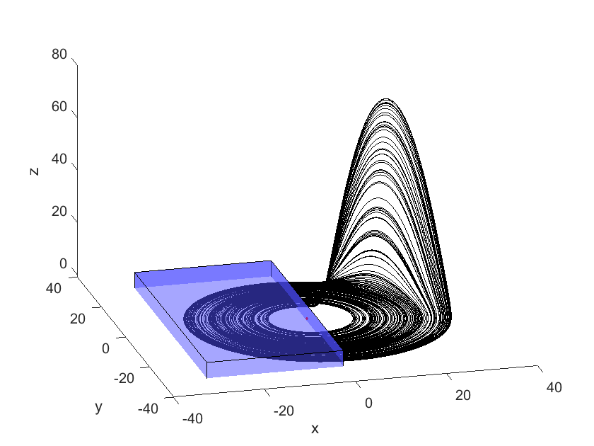
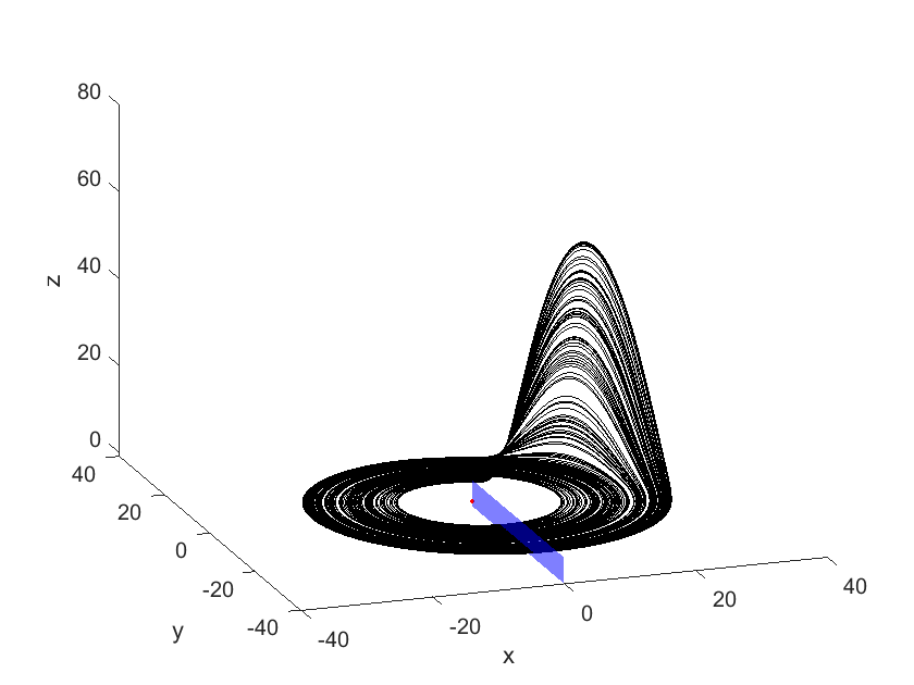
Figure 1: Up: Attractor of the velocity field $E$. The box $B$ is represented in blue. Down: Attractor of the flow generated by $\bar{f}$. The Poincaré section $\Sigma$ is represented in blue. In both cases, we took with $a=b=0.1$ and $c=18$

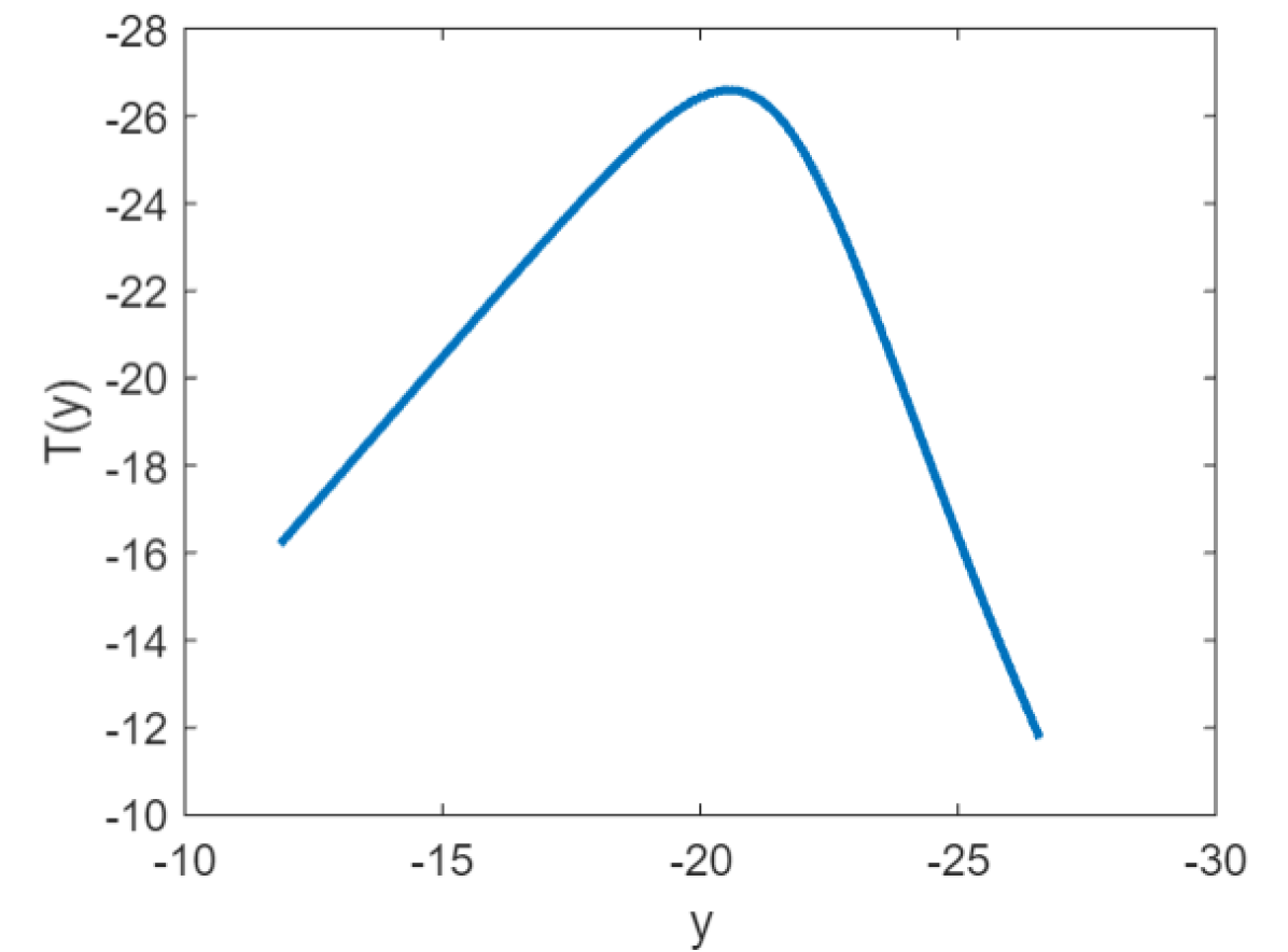
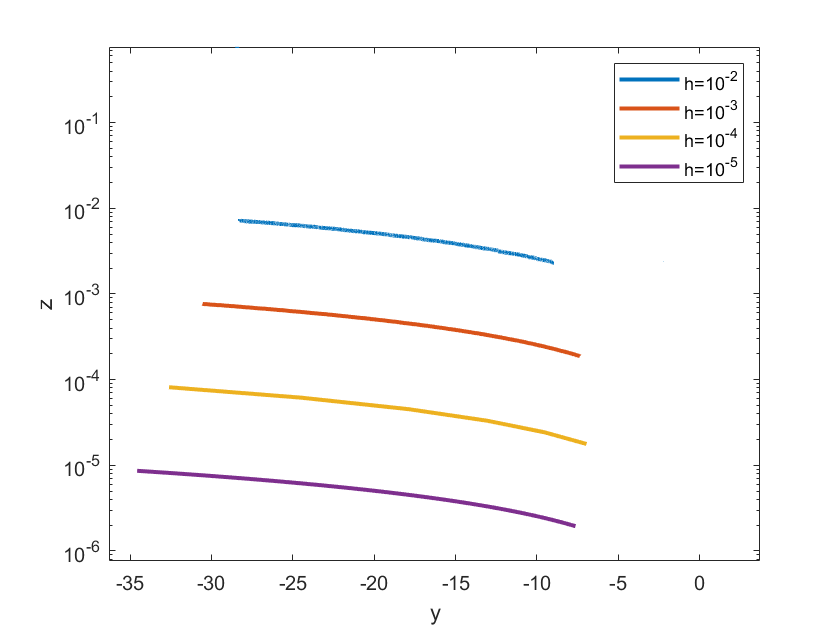
Figure 2: Left: Graphical representation of the unimodal map $\mathbf{T}$, associated with the Rössler flow of parameters $a=b=0.1$, $c=18$ (the axes are inverted). Right: 1-D cross-section of the attractor with the Poincaré section $\Sigma$ for different discretizations $h$.

This shows that the numerical estimate of the empirical average of an observable $\phi$ of the Rössler’s type semi-flow $\left(\chi_{E}^{t},t\geq 0\right)$ defined by the vector field $E$, that is the empirical average of $\phi$ computed along the trajectories of the numerically integrated system, gets very close to the expected value $\hat{\mu}\left[\phi\circ\Theta\right],$ where $\Theta$ now stands for the diffeomorphism conjugating $\left(\chi_{E}^{t},t\geq 0\right)$ with its associated suspension semi-flow and $\hat{\mu}$ is the measure with density $\frac{\mathbf{1}_{\left[0,\mathfrak{t}\right]}}{\mu_{\hat{R}}\left[\mathfrak{t}\right]}$ w.r.t. $\mu_{\hat{R}}\otimes\lambda.$ In particular this argument can be applied to estimate the generalized dimensions spectrum of the physical measure $\mu$ of the flow defined by $E$ as it will be highlighted in Remark 10 at the end of this section.

Proposition 6

Denoting $\mu_{\mathbf{T}}$ the physical measure associated with $\mathbf{T}$, we have that $D_{q}(\hat{\mu}_{R})=D_{q}(\mu_{\mathbf{T}})$ for all $q\in\mathbb{R}$, provided $D_{q}(\mu_{\mathbf{T}})$ exists.

Proof. The proof of this result is a consequence of the following lemma whose proof is deferred to the appendix.

Lemma 7

Let $I$ and $J$ be two intervals such that $I\subseteq J$ and $T:I\circlearrowleft$ a map admitting a physical measure $\mu_{T}.$ Consider the map $\hat{R}:I\times J\circlearrowleft$ such that, given $\varphi:J\circlearrowleft$ a bounded $\mathcal{B}\left(J\right)$-measurable function,

$$I\times J\ni\left(y,z\right)\longmapsto\hat{R}\left(y,z\right):=\left(T\left(y\right),\varphi\left(y\right)\right)\in I\times J\ .$$ (73)

Then, for any $f\in BL\left(I\times J\right),$ where $BL\left(I\times J\right)$ is the space of real-valued bounded Lipschitz functions on $I\times J$ of norm $1,$

$$\lim_{n\rightarrow\infty}\frac{1}{n}\sum_{k=1}^{n}f\circ\hat{R}^{k}=\mu_{T}\left[f\left(\cdot,\varphi\left(\cdot\right)\right)\right]\;,\;dydz-a.s.\ .$$ (74)

The previous lemma implies that $\hat{\mu}_{R}$ is supported on $\Gamma_{h},$ the graph of $\varphi_{h}$. Now, being

$$\mu_{\Phi}:=\mu_{\mathbf{T}}\otimes\delta_{0}\ .$$ (75)

the push-forward of $\hat{\mu}_{R}$ under the diffeomorphism

$$\mathbb{R}^{2}\ni(y,z)\longmapsto\Phi(y,z)=(y,z-\varphi_{h}(y))\in\mathbb{R}^{2}\ ,$$ (76)

we have that

$$D_{q}(\hat{\mu}_{R})=D_{q}(\mu_{\Phi})=D_{q}(\mu_{\mathbf{T}})$$ (77)

for all $q\in\mathbb{R}$ provided $D_{q}(\mu_{\mathbf{T}})$ exists.   

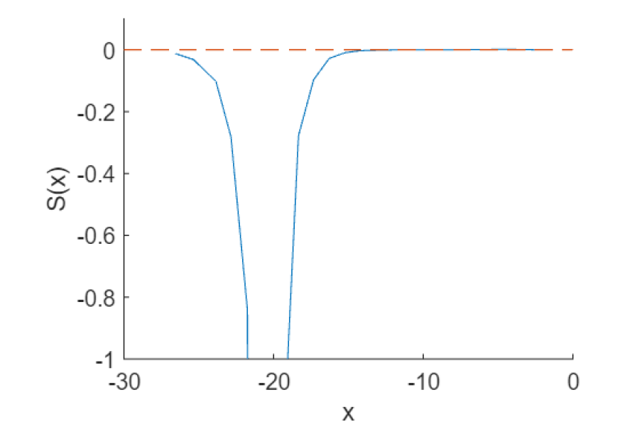
Figure 3: Schwartzian derivative of $\mathbf{T}$ for the parameters $a=b=0.1$ and $c=18$.

Let us now suppose that $\mathbf{T}$ is regular enough, so that its Schwartzian derivative $\mathbf{S}$ is well-defined outside of the critical point. This is a priori not implied by the regularity of the velocity field. Numerical simulations suggest that $\mathbf{S}$ is negative, at least for the set of parameters considered (See Figure 3). Under these assumptions, one can refer to the well-developed theory of S-unimodal maps to compute the generalized dimension spectrum of $\mu_{\mathbf{T}}$. Depending on the parameters $a$, $b$ and $c,\mu_{\mathbf{T}}$ is supported on either one of these 3 types of sets [Ke]:

1. A finite union of intervals, in which case $\mu_{\mathbf{T}}$ is absolutely continuous with respect to Lebesgue,

2. A finite collection of points, in which case $\mu_{T}$ is a sum of Dirac measures,

3. A Cantor set.

For our choice of parameters $a$, $b$ and $c$, we can reasonably rule out the second possibility, for otherwise the dynamics of the Rössler system would be periodic.
Sets of type 1) and 3) can be hard to distinguish from numerical simulations, so, in order to discriminate between the two, we estimate numerically the Lyapunov exponent

$$\lambda_{\mathbf{T}}(y)=\lim_{n\to\infty}\frac{1}{n}\sum_{i=1}^{n}\log|\mathbf{T}^{\prime}(\mathbf{T}^{i}(y))|,$$

for different generic points $y$ in the domain of $\mathbf{T}.$ The value of $\lambda_{\mathbf{T}}(y)$ turns out to be independent on the particular choice of $y$ and to be positive ($\approx 0.36$). From [Ke], $\mu_{\mathbf{T}}$ must therefore be supported on a set of type 1) rather than on a set of type 3) (which only occurs for a subset of parameters of zero Lebesgue measure in the set of parameters of $S-$unimodal maps [Ke]). It is known that under such assumptions, the density is bounded away from 0 on its support and contains singularities distributed along the orbit of the critical point [AM]. In particular, $\mu_{\mathbf{T}}$ should satisfy the hypothesis of the following Theorem (whose proof can be found in the appendix), which allows us to compute $D_{q}(\mu_{\mathbf{T}})$ explicitly.

Theorem 8

Let $I\subset\mathbb{R}$ an interval and $\nu$ a probability measure on $\left(I,\mathcal{B}(I)\right)$ that is absolutely continuous with respect to Lebesgue with a density $\rho:I\to\mathbb{R}^{+}$. Suppose $\rho$ is bounded away from $0$ in its support and of the form

$$\rho=\psi_{0}+\sum_{k=1}^{\infty}\frac{\psi_{k}\chi_{k}}{|x-x_{k}|^{\alpha_{k}}}\ ,$$ (78)

where $\{x_{k}\}_{k\geq 1}\subset I$ and, for any $k\geq 1,$

• $0<\alpha_{k+1}\leq\alpha_{k}<1.$

• $\psi_{k}$ is continuous at $x_{k}$ and $\psi_{k}(x_{k})\neq 0.$

• $\chi_{k}$ is either $\mathbf{1}_{[x_{k},+\infty)}$ or $\mathbf{1}_{(-\infty,x_{k}]}.$

Then denoting $\alpha=\underset{k\geq 1}{\sup}\{\alpha_{k}\}=\alpha_{1},$ we have

$$D_{q}(\nu)=\begin{cases}1\ \text{if}\ q<1/\alpha,\\ \frac{q(1-\alpha)}{q-1}\ \text{otherwise}.\end{cases}$$ (79)

Remark 9

For certain quadratic maps of Benedicks-Carleson type, $\alpha_{k}=1/2$ for all $k$ [BS]. For such maps, we computed in [CGSV] a quantity obtained by taking the Legendre transform of the singularity spectrum $\mathbb{R}\ni\alpha\longmapsto f(\alpha)\in\mathbb{R}$ of the measure $\nu$. This quantity is known to coincide with $\mathbb{R}\ni q\longmapsto D_{q}\in\mathbb{R}$ under some conditions on $f$ which are not verified in the present context (in particular, $f$ must be defined on an interval [Pe]). Remarkably, our formula agrees with the quantity computed in [CGSV], even though we are in the presence of countably infinitely many singularities, suggesting that this computation method remains valid in a broader context.

Applying Theorem 2, we get the following formula:

$$D_{q}(\hat{\mu})=\begin{cases}2\ \text{if}\ q<1/\alpha,\\ 1+\frac{q(1-\alpha)}{q-1}\ \text{otherwise}\ .\end{cases}$$ (80)

Estimates of $D_{q}$ for negative $q$ are known to be subject to important statistical errors [PSR], which could explain the discrepancy between the curve in Figure 1 in [L2] and Formula (80) in this range. Several publications give estimates of the correlation dimension $D_{2}(\hat{\mu})$ and of the Haussdorff dimension $D_{0}(\hat{\mu})$ that are compatible with Formula (80), with $\alpha=1/2$. For example, [SR] gives $D_{2}(\hat{\mu})=1.986\pm 0.078.$ Although these estimates are obtained for the parameters $a=0.1,b=0.1,c=14$, Formula (80) still holds if $\mathbf{T}$ is a regular $S-$unimodal map and $\mu_{\mathbf{T}}$ is absolutely continuous. We believe that it is a generic situation for choices of $a,b,c$ such that the Rössler system is chaotic, since the set of unimodal maps having a Cantor set as an attractor has zero Lebesgue measure in the set of parametrizable S-unimodal maps. The values of these parameters may possibly influence the value of $\alpha$.

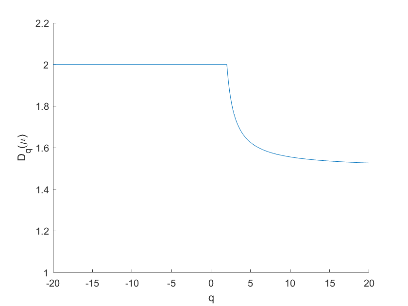
Figure 4: Representation of the $D_{q}$ spectrum of the measure $\hat{\mu}$, as given by formula (80) for $\alpha=1/2$.

Remark 10

1. Actually, $R$ is a two-dimensional map and the support of $\mu_{R}$ should exhibit a fractal structure in the $z$ direction, although invisible in numerical experiments. The contribution of this vertical component should increase the values of $D_{q}(\mu)$, so that

   $$D_{q}(\mu)\geq D_{q}(\hat{\mu}).$$

2. For simplicity, our analysis has been carried on for the velocity field $E$, but the same considerations apply to the original Rössler field $f_{c}$.

3. For values of $a,b,c$ such that the Rössler system evolves toward a periodic orbit, the invariant measure associated with the return map is a sum of Dirac measures, so that $D_{q}(\mu_{R})=0$ for all $q$. In that case, Theorem 2 yields $D_{q}(\mu)=1$ for all $q$, as expected for a measure supported on a closed curve.

3.1 Lorenz ’63 system

Since the Lorenz ’63 system is diffeomorphically conjugated to its geometric model, its generalized dimensions are those of the latter. The details of its construction can be found in [AP]. In particular, the Poincaré application is of the form

$$F(x,y)=\left(f(x),g(x,y)\right)\ ,$$ (81)

where $|g|$ is not anymore negligible as in the Rössler case. Little is known about the generalized dimensions of the physical invariant measure $\mu_{F}$ associated with $F$, whose support exhibits a fractal structure in the stable direction. However, since $\mu_{F}$ is exact dimensional [GP], by point 2. and 3. of Theorem 2 it follows that the information $D_{1}$ of the classical Lorenz system’s physical measure is well-defined and satisfies

$$D_{1}=D_{1}(\mu_{F})+1\ .$$ (82)

An explicit formula relates $D_{1}(\mu_{F})$ to the entropy and to the expanding properties of $F$ [GP].

4 Appendix

4.1 Proof of Proposition 3

The proof of Proposition 3 relies on the following lemmata.

Lemma 11

Let

$$\nu_{R}\left(d\xi\right):=\mu_{R}\left(d\xi\right)\frac{\mathfrak{t}\left(\xi\right)}{\mu_{R}\left[\mathfrak{t}\right]}\ .$$ (83)

Then, for $q\neq 1$

$$D_{q}\left(\nu_{R}\right)=D_{q}\left(\mu_{R}\right)\ .$$ (84)

Proof. Let $q>1.$ Since there exists $\kappa>0$ such that, $\kappa\leq\mathfrak{t\leq}\frac{1}{\kappa},$ we have

$$\int_{\Sigma}\nu_{R}\left(d\xi\right)\nu_{R}^{q-1}\left(B_{r}^{\left(d-1\right)}\left(\xi\right)\right) \leq\frac{1}{\left\{\kappa\mu_{R}\left[\mathfrak{t}\right]\right\}^{q}}\int_{\Sigma}\mu_{R}\left(d\xi\right)\mu_{R}^{q-1}\left(B_{r}^{\left(d-1\right)}\left(\xi\right)\right)\ ,$$ (85)

$$\int_{\Sigma}\nu_{R}\left(d\xi\right)\nu_{R}^{q-1}\left(B_{r}^{\left(d-1\right)}\left(\xi\right)\right) \geq\left\{\frac{\kappa}{\mu_{R}\left[\mathfrak{t}\right]}\right\}^{q}\int_{\Sigma}\mu_{R}\left(d\xi\right)\mu_{R}^{q-1}\left(B_{r}^{\left(d-1\right)}\left(\xi\right)\right)\ .$$ (86)

Similarly, if $q<1,$

$$\int_{\Sigma}\nu_{R}\left(d\xi\right)\nu_{R}^{q-1}\left(B_{r}^{\left(d-1\right)}\left(\xi\right)\right)=\int_{\Sigma}\nu_{R}\left(d\xi\right)\frac{1}{\nu_{R}^{1-q}\left(B_{r}^{\left(d-1\right)}\left(\xi\right)\right)}$$ (87)

$$\leq\frac{1}{\kappa\mu_{R}\left[\mathfrak{t}\right]}\frac{\mu_{R}^{1-q}\left[\mathfrak{t}\right]}{\kappa^{1-q}}\int_{\Sigma}\mu_{R}\left(d\xi\right)\frac{1}{\mu_{R}^{1-q}\left(B_{r}^{\left(d-1\right)}\left(\xi\right)\right)}$$

$$=\left\{\frac{\kappa}{\mu_{R}\left[\mathfrak{t}\right]}\right\}^{q}\int_{\Sigma}\mu_{R}\left(d\xi\right)\mu_{R}^{q-1}\left(B_{r}^{\left(d-1\right)}\left(\xi\right)\right)\ ,$$

$$\int_{\Sigma}\nu_{R}\left(d\xi\right)\frac{1}{\nu_{R}^{1-q}\left(B_{r}^{\left(d-1\right)}\left(\xi\right)\right)}\geq\frac{1}{\left\{\kappa\mu_{R}\left[\mathfrak{t}\right]\right\}^{q}}\int_{\Sigma}\mu_{R}\left(d\xi\right)\mu_{R}^{q-1}\left(B_{r}^{\left(d-1\right)}\left(\xi\right)\right)\ .$$ (88)

 

Given $r$ sufficiently small, there exists $c>1$ and $\left(\xi,t\right)\in\Sigma_{\mathfrak{t}}$ such that

$$\Theta\left(B_{c^{-1}r}^{\left(d-1\right)}\left(\xi\right)\times B_{c^{-1}r}^{\left(1\right)}\left(t\right)\right)\subseteq B_{r}^{\left(d\right)}\left(\Theta\left(t,\xi\right)\right)\subseteq\Theta\left(B_{cr}^{\left(d-1\right)}\left(\xi\right)\times B_{cr}^{\left(1\right)}\left(t\right)\right)\ .$$ (89)

Then, for $q>1,$

$$\mu\left[\mu^{q-1}\left(B_{r}^{\left(d\right)}\left(\mathbf{\cdot}\right)\right)\right]\leq\mu\left[\mu^{q-1}\left(\Theta\left(B_{cr}^{\left(d-1\right)}\left(\pi_{2}\circ\Theta^{-1}\left(\mathbf{\cdot}\right)\right)\times B_{cr}^{\left(1\right)}\left(\pi_{1}\circ\Theta^{-1}\left(\mathbf{\cdot}\right)\right)\right)\right)\right]$$ (90)

$$=\Theta_{\ast}\mu_{S}\left[\left(\Theta_{\ast}\mu_{S}\right)^{q-1}\left(\Theta\left(B_{cr}^{\left(d-1\right)}\left(\pi_{2}\circ\Theta^{-1}\left(\mathbf{\cdot}\right)\right)\times B_{cr}^{\left(1\right)}\left(\pi_{1}\circ\Theta^{-1}\left(\mathbf{\cdot}\right)\right)\right)\right)\right]$$

$$=\mu_{S}\left[\left(\Theta_{\ast}\mu_{S}\right)^{q-1}\left(\Theta\left(B_{cr}^{\left(d-1\right)}\left(\pi_{2}\left(\mathbf{\cdot}\right)\right)\times B_{cr}^{\left(1\right)}\left(\pi_{1}\left(\mathbf{\cdot}\right)\right)\right)\right)\right]$$

$$=\mu_{S}\left[\mu_{S}^{q-1}\left(B_{cr}^{\left(d-1\right)}\left(\pi_{2}\left(\cdot\right)\right)\times B_{cr}^{\left(1\right)}\left(\pi_{1}\left(\cdot\right)\right)\right)\right]$$

$$=\int_{\Sigma}\mu_{R}\left(d\xi\right)\frac{\int_{0}^{\mathfrak{t}\left(\xi\right)}dt}{\mu_{R}\left[\mathfrak{t}\right]}\left\{\int_{\Sigma}\mu_{R}\left(d\eta\right)\frac{\int_{0}^{\mathfrak{t}\left(\eta\right)}ds}{\mu_{R}\left[\mathfrak{t}\right]}\mathbf{1}_{B_{cr}^{\left(1\right)}\left(t\right)}\left(s\right)\mathbf{1}_{B_{cr}^{\left(d-1\right)}\left(\xi\right)}\left(\eta\right)\right\}^{q-1}$$

$$=\int_{\Sigma}\mu_{R}\left(d\xi\right)\frac{\int_{0}^{\mathfrak{t}\left(\xi\right)}dt}{\mu_{R}^{q}\left[\mathfrak{t}\right]}\times$$

$$\times\left\{\int_{\Sigma}\mu_{R}\left(d\eta\right)\mathbf{1}_{B_{cr}^{\left(d-1\right)}\left(\xi\right)}\left(\eta\right)\left(\mathfrak{t}\left(\eta\right)\wedge\left(t+cr\right)-\left(t-cr\right)\vee 0\right)\right\}^{q-1}\ .$$

Let us set

$$\mathfrak{t}_{\varkappa r}\left(\xi\right):=\frac{\int_{B_{\varkappa r}^{\left(d-1\right)}\left(\xi\right)}\mu_{R}\left(d\eta\right)\mathfrak{t}\left(\eta\right)}{\mu_{R}\left(B_{\varkappa r}^{\left(d-1\right)}\left(\xi\right)\right)}\;,\varkappa>0,\ .$$ (91)

We get

$$\mu\left[\mu^{q-1}\left(B_{r}^{\left(d\right)}\left(\cdot\right)\right)\right] \leq\int_{\Sigma}\mu_{R}\left(d\xi\right)\mu_{R}^{q-1}\left(B_{cr}^{\left(d-1\right)}\left(\xi\right)\right)\frac{\int_{0}^{\mathfrak{t}\left(\xi\right)}dt}{\mu_{R}^{q}\left[\mathfrak{t}\right]}\times$$ (92)

$$\times\left\{\mathfrak{t}_{cr}\left(\xi\right)\wedge\left(t+cr\right)-\left(t-cr\right)\vee 0\right\}^{q-1}\ .$$

Similarly we have

$$\mu\left[\mu^{q-1}\left(B_{r}^{\left(d\right)}\left(\cdot\right)\right)\right] \geq\int_{\Sigma}\mu_{R}\left(d\xi\right)\mu_{R}^{q-1}\left(B_{c^{-1}r}^{\left(d-1\right)}\left(\xi\right)\right)\frac{\int_{0}^{\mathfrak{t}\left(\xi\right)}dt}{\mu_{R}^{q}\left[\mathfrak{t}\right]}\times$$ (93)

$$\times\left\{\mathfrak{t}_{c^{-1}r}\left(\xi\right)\wedge\left(t+c^{-1}r\right)-\left(t-c^{-1}r\right)\vee 0\right\}^{q-1}\ .$$

Moreover, for $q<1,$ (89) implies

$$\mu\left[\mu^{q-1}\left(B_{r}^{\left(d\right)}\left(\cdot\right)\right)\right] \leq\int_{\Sigma}\mu_{R}\left(d\xi\right)\mu_{R}^{q-1}\left(B_{c^{-1}r}^{\left(d-1\right)}\left(\xi\right)\right)\frac{\int_{0}^{\mathfrak{t}\left(\xi\right)}dt}{\mu_{R}^{q}\left[\mathfrak{t}\right]}\times$$ (94)

$$\times\left\{\mathfrak{t}_{c^{-1}r}\left(\xi\right)\wedge\left(t+c^{-1}r\right)-\left(t-c^{-1}r\right)\vee 0\right\}^{q-1}$$

and

$$\mu\left[\mu^{q-1}\left(B_{r}^{\left(d\right)}\left(\cdot\right)\right)\right] \geq\int_{\Sigma}\mu_{R}\left(d\xi\right)\mu_{R}^{q-1}\left(B_{cr}^{\left(d-1\right)}\left(\xi\right)\right)\frac{\int_{0}^{\mathfrak{t}\left(\xi\right)}dt}{\mu_{R}^{q}\left[\mathfrak{t}\right]}\times$$ (95)

$$\times\left\{\mathfrak{t}_{cr}\left(\xi\right)\wedge\left(t+cr\right)-\left(t-cr\right)\vee 0\right\}^{q-1}\ .$$

Since for $r$ sufficiently small, $\varkappa>0,$

$$\mathfrak{t}_{\varkappa r}\left(\xi\right)\wedge\left(t+\varkappa r\right)-\left(t-\varkappa r\right)\vee 0=\left\{\begin{array}[]{c}\mathfrak{t}_{\varkappa r}\left(\xi\right)-t+\varkappa r\\ 2\varkappa r\\ t+\varkappa r\end{array}\right.\ ,$$ (96)

we have

Lemma 12

For $q\neq 1,$

$$\lim_{r\downarrow 0}\frac{\log\int_{\Sigma}\mu_{R}\left(d\xi\right)\mu_{R}^{q-1}\left(B_{cr}^{\left(d-1\right)}\left(\xi\right)\right)\frac{\int_{0}^{\mathfrak{t}\left(\xi\right)}dt\left[\mathfrak{t}_{cr}\left(\xi\right)-t+cr\right]^{q-1}}{\mu_{R}^{q}\left[\mathfrak{t}\right]}}{\log r}$$ (97)

$$=\lim_{r\downarrow 0}\frac{\log\int_{\Sigma}\mu_{R}\left(d\xi\right)\mu_{R}^{q-1}\left(B_{c^{-1}r}^{\left(d-1\right)}\left(\xi\right)\right)\frac{\int_{0}^{\mathfrak{t}\left(\xi\right)}dt\left[\mathfrak{t}_{c^{-1}r}\left(\xi\right)-t+c^{-1}r\right]^{q-1}}{\mu_{R}^{q}\left[\mathfrak{t}\right]}}{\log r}$$

$$=\left(q-1\right)D_{q}\left(\nu_{R}\right)\ .$$

Proof. Let us consider first the case $q>1.$

Denoting by $s:=\mathfrak{t}_{cr}\left(\xi\right)-t+cr,$ for some $\lambda_{r}\in\left[0,1\right]$ such that $\lim_{r\downarrow 0}\lambda_{r}=1,$

$$\int_{\Sigma}\mu_{R}\left(d\xi\right)\mu_{R}^{q-1}\left(B_{cr}^{\left(d-1\right)}\left(\xi\right)\right)\frac{\int_{0}^{\mathfrak{t}\left(\xi\right)}dt\left[\mathfrak{t}_{cr}\left(\xi\right)-t+cr\right]^{q-1}}{\mu_{R}^{q}\left[\mathfrak{t}\right]}$$ (98)

$$=\int_{\Sigma}\mu_{R}\left(d\xi\right)\mu_{R}^{q-1}\left(B_{cr}^{\left(d-1\right)}\left(\xi\right)\right)\frac{\int_{\mathfrak{t}_{cr}\left(\xi\right)-\mathfrak{t}\left(\xi\right)+cr}^{\mathfrak{t}_{cr}\left(\xi\right)+cr}s^{q-1}ds}{\mu_{R}^{q}\left[\mathfrak{t}\right]}$$

$$=\int_{\Sigma}\mu_{R}\left(d\xi\right)\mu_{R}^{q-1}\left(B_{cr}^{\left(d-1\right)}\left(\xi\right)\right)\times$$

$$\times\frac{\mathfrak{t}\left(\xi\right)\left[\lambda_{cr}\left(\mathfrak{t}_{cr}\left(\xi\right)+cr\right)+\left(1-\lambda_{r}\right)\left(\mathfrak{t}_{cr}\left(\xi\right)+cr-\mathfrak{t}\left(\xi\right)\right)\right]^{q-1}}{\mu_{R}^{q}\left[\mathfrak{t}\right]}$$

$$\leq\frac{1}{\kappa^{q-1}}\int_{\Sigma}\nu_{R}\left(d\xi\right)\nu_{R}^{q-1}\left(B_{cr}^{\left(d-1\right)}\left(\xi\right)\right)\times$$

$$\times\left[\lambda_{r}\left(\mathfrak{t}_{cr}\left(\xi\right)+cr\right)+\left(1-\lambda_{r}\right)\left(\mathfrak{t}_{cr}\left(\xi\right)+cr-\mathfrak{t}\left(\xi\right)\right)\right]^{q-1}$$

$$=\frac{1}{\kappa^{q-1}}\int_{\Sigma}\nu_{R}\left(d\xi\right)\nu_{R}^{q-1}\left(B_{cr}^{\left(d-1\right)}\left(\xi\right)\right)\left[\mathfrak{t}_{cr}\left(\xi\right)+cr+\left(\lambda_{r}-1\right)\mathfrak{t}\left(\xi\right)\right]^{q-1}\ .$$

Since $\mathfrak{t}$ has bounded variation,

$$\left|\mathfrak{t}_{\varkappa r}\left(\cdot\right)-\mathfrak{t}\left(\cdot\right)\right| \leq\frac{\int_{B_{\varkappa r}^{\left(d-1\right)}\left(\cdot\right)}\mu_{R}\left(d\eta\right)\left|\mathfrak{t}\left(\eta\right)-\mathfrak{t}\left(\cdot\right)\right|}{\mu_{R}\left(B_{\varkappa r}^{\left(d-1\right)}\left(\cdot\right)\right)}$$ (99)

$$\leq 2r\sup_{\eta\in B_{\varkappa r}^{\left(d-1\right)}\left(\cdot\right)}\left|\nabla\mathfrak{t}\left(\eta\right)\right|\ .$$

Thus, there exists $c^{\prime}>0$ such that $\left|\mathfrak{t}_{\varkappa r}\left(\cdot\right)-\mathfrak{t}\left(\cdot\right)\right|\leq c^{\prime}r,$ so that

$$\kappa+O\left(r\right)\leq\left[\mathfrak{t}_{cr}\left(\xi\right)+cr+\left(\lambda_{r}-1\right)\mathfrak{t}\left(\xi\right)\right]\leq\frac{1}{\kappa}+O\left(r\right)\ ;$$ (100)

which implies,

$$\int_{\Sigma}\nu_{R}\left(d\xi\right)\nu_{R}^{q-1}\left(B_{cr}^{\left(d-1\right)}\left(\xi\right)\right)\left[\mathfrak{t}_{cr}\left(\xi\right)-\mathfrak{t}\left(\xi\right)+cr+\lambda_{r}\mathfrak{t}\left(\xi\right)\right]^{q-1}$$ (101)

$$\leq\frac{1}{\kappa^{q-1}}\left(\frac{1}{\kappa}+O\left(r\right)\right)^{q-1}\int_{\Sigma}\nu_{R}\left(d\xi\right)\nu_{R}^{q-1}\left(B_{cr}^{\left(d-1\right)}\left(\xi\right)\right)$$

$$=\frac{1}{\kappa^{q-1}}\left[\frac{1}{\kappa^{q-1}}+O\left(r\right)\right]\int_{\Sigma}\nu_{R}\left(d\xi\right)\nu_{R}^{q-1}\left(B_{cr}^{\left(d-1\right)}\left(\xi\right)\right)\ .$$

On the other hand,

$$\int_{\Sigma}\mu_{R}\left(d\xi\right)\mu_{R}^{q-1}\left(B_{c^{-1}r}^{\left(d-1\right)}\left(\xi\right)\right)\frac{\int_{\mathfrak{t}_{r}\left(\xi\right)-\mathfrak{t}\left(\xi\right)+c^{-1}r}^{\mathfrak{t}_{r}\left(\xi\right)+c^{-1}r}s^{q-1}ds}{\mu_{R}^{q}\left[\mathfrak{t}\right]}$$ (102)

$$\geq\kappa^{q-1}\int_{\Sigma}\nu_{R}\left(d\xi\right)\nu_{R}^{q-1}\left(B_{c^{-1}r}^{\left(d-1\right)}\left(\xi\right)\right)\left[\mathfrak{t}_{c^{-1}r}\left(\xi\right)-\mathfrak{t}\left(\xi\right)+c^{-1}r+\lambda_{r}\mathfrak{t}\left(\xi\right)\right]^{q-1}$$

$$\geq\kappa^{q-1}\left[\lambda_{r}\kappa^{q-1}+O\left(r\right)\right]\int_{\Sigma}\nu_{R}\left(d\xi\right)\nu_{R}^{q-1}\left(B_{c^{-1}r}^{\left(d-1\right)}\left(\xi\right)\right)\ .$$

Similarly for $q<1$ we have

$$\int_{\Sigma}\mu_{R}\left(d\xi\right)\mu_{R}^{q-1}\left(B_{c^{-1}r}^{\left(d-1\right)}\left(\xi\right)\right)\frac{\int_{0}^{\mathfrak{t}\left(\xi\right)}dt\frac{1}{\left[\mathfrak{t}_{c^{-1}r}\left(\xi\right)-t+c^{-1}r\right]^{1-q}}}{\mu_{R}^{q}\left[\mathfrak{t}\right]}$$ (103)

$$\leq\frac{1}{\kappa^{q-1}}\int_{\Sigma}\nu_{R}\left(d\xi\right)\nu_{R}^{q-1}\left(B_{c^{-1}r}^{\left(d-1\right)}\left(\xi\right)\right)\frac{1}{\left[\mathfrak{t}_{c^{-1}r}\left(\xi\right)+c^{-1}r+\left(\lambda_{r}-1\right)\mathfrak{t}\left(\xi\right)\right]^{1-q}}$$

$$\leq\frac{1}{\kappa^{q-1}}\frac{1}{\left[\lambda_{r}\kappa+O\left(r\right)\right]^{1-q}}\int_{\Sigma}\nu_{R}\left(d\xi\right)\nu_{R}^{q-1}\left(B_{c^{-1}r}^{\left(d-1\right)}\left(\xi\right)\right)$$

and

$$\int_{\Sigma}\mu_{R}\left(d\xi\right)\mu_{R}^{q-1}\left(B_{cr}^{\left(d-1\right)}\left(\xi\right)\right)\frac{\int_{0}^{\mathfrak{t}\left(\xi\right)}dt\frac{1}{\left[\mathfrak{t}_{cr}\left(\xi\right)-t+cr\right]^{1-q}}}{\mu_{R}^{q}\left[\mathfrak{t}\right]}$$ (104)

$$\geq\kappa^{q-1}\int_{\Sigma}\nu_{R}\left(d\xi\right)\nu_{R}^{q-1}\left(B_{cr}^{\left(d-1\right)}\left(\xi\right)\right)\frac{1}{\left[\mathfrak{t}_{cr}\left(\xi\right)-\mathfrak{t}\left(\xi\right)+cr+\lambda_{r}\mathfrak{t}\left(\xi\right)\right]^{1-q}}$$

$$\geq\kappa^{q-1}\frac{1}{\left[\kappa^{-1}+O\left(r\right)\right]^{1-q}}\int_{\Sigma}\nu_{R}\left(d\xi\right)\nu_{R}^{q-1}\left(B_{cr}^{\left(d-1\right)}\left(\xi\right)\right)\ .$$

 

Lemma 13

For $q\neq 1,$

$$\lim_{r\downarrow 0}\frac{\log\int_{\Sigma}\mu_{R}\left(d\xi\right)\mu_{R}^{q-1}\left(B_{cr}^{\left(d-1\right)}\left(\xi\right)\right)\frac{\int_{0}^{\mathfrak{t}\left(\xi\right)}dt\left[t+cr\right]^{q-1}}{\mu_{R}^{q}\left[\mathfrak{t}\right]}}{\log r}$$ (105)

$$=\lim_{r\downarrow 0}\frac{\log\int_{\Sigma}\mu_{R}\left(d\xi\right)\mu_{R}^{q-1}\left(B_{c^{-1}r}^{\left(d-1\right)}\left(\xi\right)\right)\frac{\int_{0}^{\mathfrak{t}\left(\xi\right)}dt\left[t+c^{-1}r\right]^{q-1}}{\mu_{R}^{q}\left[\mathfrak{t}\right]}}{\log r}$$

$$=\left(q-1\right)D_{q}\left(\nu_{R}\right)\ .$$

Proof. Let $q>1.$ Denoting by $s:=t+cr,$ for some $\lambda_{r}\in\left[0,1\right]$ such that $\lim_{r\downarrow 0}\lambda_{r}=1,$

$$\int_{\Sigma}\mu_{R}\left(d\xi\right)\mu_{R}^{q-1}\left(B_{cr}^{\left(d-1\right)}\left(\xi\right)\right)\frac{\int_{0}^{\mathfrak{t}\left(\xi\right)}dt\left[t+cr\right]^{q-1}}{\mu_{R}^{q}\left[\mathfrak{t}\right]}$$ (106)

$$=\int_{\Sigma}\mu_{R}\left(d\xi\right)\mu_{R}^{q-1}\left(B_{cr}^{\left(d-1\right)}\left(\xi\right)\right)\frac{\int_{cr}^{\mathfrak{t}\left(\xi\right)+cr}dss^{q-1}}{\mu_{R}^{q}\left[\mathfrak{t}\right]}$$

$$=\int_{\Sigma}\mu_{R}\left(d\xi\right)\mu_{R}^{q-1}\left(B_{cr}^{\left(d-1\right)}\left(\xi\right)\right)\frac{\mathfrak{t}\left(\xi\right)\left[\lambda_{r}\left(\mathfrak{t}\left(\xi\right)+cr\right)+\left(1-\lambda_{r}\right)\left(cr\right)\right]^{q-1}}{\mu_{R}^{q}\left[\mathfrak{t}\right]}$$

$$\leq\frac{1}{\kappa^{q-1}}\int_{\Sigma}\nu_{R}\left(d\xi\right)\nu_{R}^{q-1}\left(B_{cr}^{\left(d-1\right)}\left(\xi\right)\right)\left[\lambda_{r}\mathfrak{t}\left(\xi\right)+cr\right]^{q-1}$$

$$\leq\frac{\left[\kappa^{-1}+cr\right]^{q-1}}{\kappa^{q-1}}\int_{\Sigma}\nu_{R}\left(d\xi\right)\nu_{R}^{q-1}\left(B_{cr}^{\left(d-1\right)}\left(\xi\right)\right)\ .$$

Similarly,

$$\int_{\Sigma}\mu_{R}\left(d\xi\right)\mu_{R}^{q-1}\left(B_{c^{-1}r}^{\left(d-1\right)}\left(\xi\right)\right)\frac{\int_{0}^{\mathfrak{t}\left(\xi\right)}dt\left[t+c^{-1}r\right]^{q-1}}{\mu_{R}^{q}\left[\mathfrak{t}\right]}$$ (107)

$$\geq\kappa^{q-1}\int_{\Sigma}\nu_{R}\left(d\xi\right)\nu_{R}^{q-1}\left(B_{c^{-1}r}^{\left(d-1\right)}\left(\xi\right)\right)\left[\lambda_{r}\mathfrak{t}\left(\xi\right)+c^{-1}r\right]^{q-1}$$

$$\geq\left[\lambda_{r}\kappa+c^{-1}r\right]^{q-1}\kappa^{q-1}\int_{\Sigma}\nu_{R}\left(d\xi\right)\nu_{R}^{q-1}\left(B_{c^{-1}r}^{\left(d-1\right)}\left(\xi\right)\right)\ .$$

On the other hand, for $q<1,$

$$\int_{\Sigma}\mu_{R}\left(d\xi\right)\mu_{R}^{q-1}\left(B_{c^{-1}r}^{\left(d-1\right)}\left(\xi\right)\right)\frac{\int_{0}^{\mathfrak{t}\left(\xi\right)}dt\frac{1}{\left[t+c^{-1}r\right]^{1-q}}}{\mu_{R}^{q}\left[\mathfrak{t}\right]}$$ (108)

$$\leq\frac{1}{\kappa^{q-1}}\int_{\Sigma}\nu_{R}\left(d\xi\right)\nu_{R}^{q-1}\left(B_{c^{-1}r}^{\left(d-1\right)}\left(\xi\right)\right)\frac{1}{\left[\lambda_{r}\mathfrak{t}\left(\xi\right)+c^{-1}r\right]^{1-q}}$$

$$\leq\frac{1}{\kappa^{q-1}\left[\lambda_{r}\kappa+c^{-1}r\right]^{1-q}}\int_{\Sigma}\nu_{R}\left(d\xi\right)\nu_{R}^{q-1}\left(B_{cr}^{\left(d-1\right)}\left(\xi\right)\right)\ .$$

 

Lemma 14

For $q\neq 1,$

$$\lim_{r\downarrow 0}\frac{\log\int_{\Sigma}\mu_{R}\left(d\xi\right)\mu_{R}^{q-1}\left(B_{cr}^{\left(d-1\right)}\left(\xi\right)\right)\frac{\int_{0}^{\mathfrak{t}\left(\xi\right)}dt\left[2cr\right]^{q-1}}{\mu_{R}^{q}\left[\mathfrak{t}\right]}}{\log r}$$ (109)

$$=\lim_{r\downarrow 0}\frac{\log\int_{\Sigma}\mu_{R}\left(d\xi\right)\mu_{R}^{q-1}\left(B_{c^{-1}r}^{\left(d-1\right)}\left(\xi\right)\right)\frac{\int_{0}^{\mathfrak{t}\left(\xi\right)}dt\left[c^{-1}r\right]^{q-1}}{\mu_{R}^{q}\left[\mathfrak{t}\right]}}{\log r}$$

$$=\left(q-1\right)D_{q}\left(\nu_{R}\right)+q-1\ .$$

Proof.

$$\int_{\Sigma}\mu_{R}\left(d\xi\right)\mu_{R}^{q-1}\left(B_{cr}^{\left(d-1\right)}\left(\xi\right)\right)\frac{\int_{0}^{\mathfrak{t}\left(\xi\right)}dt\left[2cr\right]^{q-1}}{\mu_{R}^{q}\left[\mathfrak{t}\right]}$$ (110)

$$=\left[2cr\right]^{q-1}\int_{\Sigma}\mu_{R}\left(d\xi\right)\mu_{R}^{q-1}\left(B_{cr}^{\left(d-1\right)}\left(\xi\right)\right)\frac{\mathfrak{t}\left(\xi\right)}{\mu_{R}^{q}\left[\mathfrak{t}\right]}$$

$$\leq\left[\frac{2cr}{\kappa}\right]^{q-1}\int_{\Sigma}\nu_{R}\left(d\xi\right)\nu_{R}^{q-1}\left(B_{cr}^{\left(d-1\right)}\left(\xi\right)\right)$$

and

$$\int_{\Sigma}\mu_{R}\left(d\xi\right)\mu_{R}^{q-1}\left(B_{cr}^{\left(d-1\right)}\left(\xi\right)\right)\frac{\int_{0}^{\mathfrak{t}\left(\xi\right)}dt\left[2cr\right]^{q-1}}{\mu_{R}^{q}\left[\mathfrak{t}\right]}$$ (111)

$$\geq\left[2cr\kappa\right]^{q-1}\int_{\Sigma}\nu_{R}\left(d\xi\right)\nu_{R}^{q-1}\left(B_{cr}^{\left(d-1\right)}\left(\xi\right)\right)\ ,$$

as well as

$$\int_{\Sigma}\mu_{R}\left(d\xi\right)\mu_{R}^{q-1}\left(B_{c^{-1}r}^{\left(d-1\right)}\left(\xi\right)\right)\frac{\int_{0}^{\mathfrak{t}\left(\xi\right)}dt\left[2c^{-1}r\right]^{q-1}}{\mu_{R}^{q}\left[\mathfrak{t}\right]}$$ (112)

$$\leq\left[\frac{2c^{-1}r}{\kappa}\right]^{q-1}\int_{\Sigma}\nu_{R}\left(d\xi\right)\nu_{R}^{q-1}\left(B_{c^{-1}r}^{\left(d-1\right)}\left(\xi\right)\right)\ ,$$

$$\int_{\Sigma}\mu_{R}\left(d\xi\right)\mu_{R}^{q-1}\left(B_{c^{-1}r}^{\left(d-1\right)}\left(\xi\right)\right)\frac{\int_{0}^{\mathfrak{t}\left(\xi\right)}dt\left[2c^{-1}r\right]^{q-1}}{\mu_{R}^{q}\left[\mathfrak{t}\right]}$$ (113)

$$\geq\left[2c^{-1}r\kappa\right]^{q-1}\int_{\Sigma}\nu_{R}\left(d\xi\right)\nu_{R}^{q-1}\left(B_{c^{-1}r}^{\left(d-1\right)}\left(\xi\right)\right)\ .$$

 

In view of Lemma 11, for $q\neq 1,$ Proposition 3 follows collecting the Lemmata 12, 13 and 14.

4.2 Proof of Lemma 7

Proof. Let $g$ be a positive symmetric mollifier, i.e. a smooth function such that:

• it is supported on $J;$

• if $x_{J}$ is the middle point of $J,\int dxg\left(x-x_{J}\right)=1;$

• $\forall f\in BL\left(J\right),$ setting $J\ni x\longmapsto g_{\sigma}\left(y\right):=\sigma^{-1}g_{\sigma}\left(\frac{y-y_{J}}{\sigma}\right)\in\mathbb{R}_{+},\lim_{\sigma\downarrow 0}\int dx\frac{g\left(\frac{x-x_{J}}{\sigma}\right)}{\sigma}f\left(y\right)=f\left(x_{J}\right);$

for example we may choose

$$J\ni y\longmapsto g\left(x\right):=\frac{Z_{J}}{\sqrt{2\pi}}e^{-\frac{\left(x-x_{J}\right)^{2}}{2}}\mathbf{1}_{J}\left(\left|x-x_{J}\right|\right)\in\mathbb{R}_{+}\ .$$ (114)

with $Z_{J}$ such that $\int_{J}dxg\left(x\right)=1.$ Then, $\forall f\in BL\left(I\times J\right)$ and $\left(x,y\right)\in I\times J,$ by the Schwartz inequality, we get

$$\left|\int_{J}dzg_{\sigma}\left(z-y\right)f\left(x,z\right)-f\left(x,y\right)\right| =\int_{J}dzg_{\sigma}\left(z-y\right)\left|f\left(x,z\right)-f\left(x,y\right)\right|$$ (115)

$$\leq\int_{J}dzg_{\sigma}\left(z-y\right)\left|z-y\right|$$

$$\leq\sqrt{\int_{J}dzg_{\sigma}\left(z-y\right)\left(z-y\right)^{2}}\leq Z_{J}\sigma\ ,$$

where we have used that $\forall\left(x,y\right)\in I\times J,$

$$\left|f\left(x,z\right)-f\left(x,y\right)\right|\leq\left\|f\right\|_{BL\left(I\times J\right)}\left|z-y\right|=\left|z-y\right|\ .$$ (116)

Hence, setting $\int_{J}dzg_{\sigma}\left(z-y\right)f\left(x,z\right)=:\left(g_{\sigma}\ast f\right)\left(x,y\right)$ and considering the bounded linear operators on the Banach space $BM\left(I\times J\right)$ of bounded $\mathcal{B}\left(I\times J\right)$-measurable functions endowed with the sup-norm

$$BM\left(I\times J\right) \ni f\longmapsto T_{\varphi}f\left(\cdot,\cdot\right):=f\left(\cdot,\varphi\left(\cdot\right)\right)\in BM\left(I\times J\right)\ ,$$ (117)

$$BM\left(I\times J\right) \ni f\longmapsto G_{\sigma}f:=\left(g_{\sigma}\ast f\right)\in BM\left(I\times J\right)\ ,$$ (118)

for any $f\in BM\left(I\times J\right)$ we have

$$T_{\varphi}\left(G_{\sigma}f\right)=\left(T_{\varphi}G_{\sigma}\right)f=\left(T_{\varphi}g_{\sigma}\right)\ast f=g_{\sigma}\ast\left(T_{\varphi}f\right)=G_{\sigma}\left(T_{\varphi}f\right)\ .$$ (119)

Since $\forall f\in BL\left(I\times J\right)$

$$\left|\frac{1}{n}\sum_{k=1}^{n}f\circ R^{k}-\frac{1}{n}\sum_{k=1}^{n}\left(g_{\sigma}\ast f\right)\left(T^{k}\left(x\right),\varphi\circ T^{k-1}\left(x\right)\right)\right|$$ (120)

$$\leq\frac{1}{n}\sum_{k=1}^{n}\left|f\left(T^{k}\left(x\right),\varphi\circ T^{k-1}\left(x\right)\right)-\left(g_{\sigma}\ast f\right)\left(T^{k}\left(x\right),\varphi\circ T^{k-1}\left(x\right)\right)\right|$$

$$\leq\frac{1}{n}\sum_{k=1}^{n}\int_{J}dzg_{\sigma}\left(z-\varphi\circ T^{k-1}\left(y\right)\right)\left|f\left(T^{k}\left(x\right),z\right)-f\left(T^{k}\left(x\right),\varphi\circ T^{k-1}\left(x\right)\right)\right|$$

$$\leq Z_{J}\sigma\ ,$$

we get

$$\frac{1}{n}\sum_{k=1}^{n}f\circ R^{k} =\frac{1}{n}\sum_{k=1}^{n}f\left(T^{k}\left(x\right),\varphi\circ T^{k-1}\left(x\right)\right)-\left(g_{\sigma}\ast f\right)\left(T^{k}\left(x\right),\varphi\circ T^{k-1}\left(x\right)\right)$$ (121)

$$+\frac{1}{n}\sum_{k=1}^{n}\left(g_{\sigma}\ast f\right)\left(T^{k}\left(x\right),\varphi\circ T^{k-1}\left(x\right)\right)$$

$$\leq Z_{J}\sigma+\frac{1}{n}\sum_{k=1}^{n}\left(g_{\sigma}\ast f\right)\left(T^{k}\left(x\right),\varphi\circ T^{k-1}\left(x\right)\right)$$

and

$$\frac{1}{n}\sum_{k=1}^{n}f\circ R^{k}\geq-Z_{J}\sigma+\frac{1}{n}\sum_{k=1}^{n}\left(g_{\sigma}\ast f\right)\left(T^{k}\left(x\right),\varphi\circ T^{k-1}\left(x\right)\right)\ .$$ (122)

But,

$$\frac{1}{n}\sum_{k=1}^{n}\left(g_{\sigma}\ast f\right)\left(T^{k}\left(x\right),\varphi\circ T^{k-1}\left(x\right)\right)=$$ (123)

$$=\int_{J}dz\frac{1}{n}\sum_{k=1}^{n}g_{\sigma}\left(z-T^{k-1}\left(x\right)\right)f\left(T^{k}\left(x\right),\varphi\left(z\right)\right)\underset{n\uparrow\infty}{\longrightarrow}\int_{J}dz\int_{I}\mu_{T}\left(dy\right)g_{\sigma}\left(z-y\right)f\left(y,\varphi\left(z\right)\right)\ .$$

Letting $\sigma\downarrow 0$ we obtain $\lim_{n\rightarrow\infty}\frac{1}{n}\sum_{k=1}^{n}f\circ R^{k}=\mu_{T}\left[f\left(\cdot,\varphi\left(\cdot\right)\right)\right]\ dxdy-a.s.,$ that is $R$ admits an invariant measure $\mu_{R}$ whose support is the graph of $\varphi;$ in other words $spt\mu_{R}=\left\{\left(x,y\right)\in I\times J:y=\varphi\left(x\right)\right\},$ and disintegrates as $\mu_{T}\left(dx\right)\delta_{\left\{\varphi\left(x\right)\right\}}\left(dy\right)$ where $\delta_{\left\{z\right\}}\left(dy\right)$ stands for the Dirac mass at $\left\{z\right\}.$   

We remark that, as it clearly appears from the proof, this result is independent of the choice of the mollifier $g.$

4.3 Proof of Theorem 8

We will first prove the following lemma, which deals with the case of a finite number of singularities, and then move to the infinite case.

Lemma 15

Let $I\subset\mathbb{R}$ an interval, $n\geq 1$ and $\nu$ a probability measure on $\left(I,\mathcal{B}\left(I\right)\right)$ that is absolutely continuous with respect to Lebesgue with a density $\rho_{n}:I\rightarrow\mathbb{R}^{+}$. Suppose $\rho_{n}$ is bounded away from $0$ in its support and is of the form

$$\rho_{n}=\psi_{0}+\sum_{k=1}^{n}\frac{\psi_{k}\chi_{k}}{|x-x_{k}|^{\alpha_{k}}}\ ,$$ (124)

where $\{x_{k}\}_{k=1,...,n}\subset I$ and, for any $k=1,..,n,$

• $0<\alpha_{k}<1.$

• $\psi_{k}$ is continuous at $x_{k}$ and $\psi_{k}(x_{k})\neq 0$.

• $\chi_{k}$ is either $\mathbf{1}_{[x_{k},+\infty)}$ or $\mathbf{1}_{(-\infty,x_{k}]}.$

Then denoting $\alpha:=\underset{k=1,...,n}{\max}\{\alpha_{k}\},$

$$D_{q}(\nu)=\begin{cases}1\ \text{if}\ q<1/\alpha\ ,\\ \frac{q(1-\alpha)}{q-1}\ \text{otherwise}\ .\end{cases}$$ (125)

Proof. To ease the computations, we will write the proof assuming that the terms $\psi_{k}$ and $\chi_{k}$ are set equal to $1$ for any value of $k.$ As a matter of fact, this assumption will not affect the result which, as it will clearly appear from the development of the proof, will depend only on the order of the singularities of $\rho_{n}.$ Let us denote $k_{0}$ the smallest index that realizes $\alpha_{k_{0}}=\alpha$ and set

$$I_{q}(r):=\int_{I}\nu(B_{r}(x))^{q-1}d\nu(x)\ .$$ (126)

All along the proof, $c$ and $c_{i}$ denote positive constants whose values can change from line to line.

Let us first deal with the case $q<0.$ Since

$$|x-x_{k_{0}}|^{-\alpha}\leq\rho_{n}(x)\leq c\sum_{k=1}^{n}|x-x_{k}|^{-\alpha}\ ,$$ (127)

we have

$$I_{q}(r)\leq c\sum_{l=0}^{n}\int_{I}dx(x-x_{l})^{-\alpha}\left[\int_{x-r}^{x+r}(y-x_{k_{0}})^{-\alpha}dy\right]^{q-1}\ .$$ (128)

Since, for all $k=1,...,n,$

$$\int_{x-r}^{x+r}dy|y-x_{k}|^{-\alpha}\asymp r\mathbf{1}_{B_{r}^{c}(x_{k})}(x)+\mathbf{1}_{B_{r}(x_{k})}(x)(|x-x_{k}|+r)^{1-\alpha}\ ,$$ (129)

(128) and (129) yield

$$I_{q}(r) \leq cr^{q-1}\sum_{l=1}^{n}\int_{I}dx|x-x_{l}|^{-\alpha}\mathbf{1}_{B_{r}^{c}(x_{k_{0}})}(x)+$$ (130)

$$+c\sum_{1\leq l\leq n\ :\ l\neq k_{0}}\int_{I}dx\left|x-x_{l}\right|^{-\alpha}(|x-x_{k_{0}}|+r)^{(1-\alpha)(q-1)}]\mathbf{1}_{B_{r}(x_{k_{0}})}(x)+$$

$$+c\int_{I}dx\left|x-x_{k_{0}}\right|^{-\alpha}(|x-x_{k_{0}}|+r)^{(1-\alpha)(q-1)}\mathbf{1}_{B_{r}(x_{k_{0}})}(x)\ ,$$

The integral in the first term on the r.h.s. of (130) is finite, hence this term is bounded by $c_{1}r^{q-1}.$ The second term on the r.h.s. (130) is bounded by $c_{2}r^{(1-\alpha)q+\alpha},$ while the third term is bounded by $c_{3}r^{\left(1-\alpha\right)q}.$ Therefore,

$$I_{q}(r)\leq c_{1}r^{q-1}+c_{2}r^{(1-\alpha)q+\alpha}+c_{3}r^{\left(1-\alpha\right)q}\ .$$ (131)

Since $q<0$ and $0<\alpha<1,$

$$I_{q}(r)\leq c_{1}r^{q-1}\left(1+o(r^{q-1})\right)\ ,$$ (132)

then

$$D_{q}(\nu)\geq 1\ .$$ (133)

Since $\mathbb{R}^{+}\ni x\longmapsto x^{q-1}\in\mathbb{R}$ is a convex function, by (127) and by the Jensen inequality,

$$I_{q}(r) \geq c\int_{I}dx(x-x_{k_{0}})^{-\alpha}\left[\sum_{k=0}^{n}\int_{x-r}^{x+r}(y-x_{k})^{-\alpha}dy\right]^{q-1}$$

$$\geq c\left[\sum_{k=0}^{n}\int_{I}dx(x-x_{k_{0}})^{-\alpha}\int_{x-r}^{x+r}(y-x_{k})^{-\alpha}dy\right]^{q-1}\ .$$

Thus, the upper bound of $D_{q}\left(\nu\right)$ is obtained in similar fashion combining (4.3) and (129).

Let us now consider $q>1.$ From (127) we have

$$I_{q}(r)\geq c\int_{I}dx|x-x_{k_{0}}|^{-\alpha}\left[\int_{x-r}^{x+r}|y-x_{k_{0}}|^{-\alpha}dy\right]^{q-1}\ ,$$ (135)

which yields, as for the previous cases,

$$I_{q}(r)\geq c_{1}r^{q-1}+c_{2}r^{(1-\alpha)q+\alpha}+c_{3}r^{\left(1-\alpha\right)q}\ .$$ (136)

If $q>1/\alpha,$

$$I_{q}(r)\geq c_{3}r^{\left(1-\alpha\right)q}\left(1+o(r^{\left(1-\alpha\right)q})\right)\ ,$$ (137)

which implies

$$D_{q}(\nu)\leq\frac{(1-\alpha)q}{q-1}\ .$$ (138)

On the other hand, if $1<q\leq 1/\alpha,$

$$I_{q}(r)\geq c_{1}r^{q-1}\left(1+o(r^{q-1})\right)\ ,$$ (139)

which leads to

$$D_{q}(\nu)\leq 1\ .$$ (140)

For what concerns the lower bound, we have

$$I_{q}(r) \leq c\sum_{l=0}^{n}\int_{I}dx|x-x_{l}|^{-\alpha}\left[\sum_{k=0}^{n}\int_{x-r}^{x+r}|y-x_{k}|^{-\alpha}dy\right]^{q-1}$$

$$\leq c\sum_{k,l=0}^{n}\int_{I}dx|x-x_{l}|^{-\alpha}\left[\int_{x-r}^{x+r}|y-x_{k}|^{-\alpha}dy\right]^{q-1}\ .$$

Indeed, the last inequality is obtained for $q\geq 2$ by Jensen inequality, while for $1<q<2,$ it comes from the fact that

$$(a+b)^{q-1}\leq a^{q-1}+b^{q-1}$$ (142)

for any $a,b>0.$ Combining with (129), we get

$$I_{q}(r) \leq cr^{q-1}\sum_{k,l=1}^{n}\int_{I}dx|x-x_{l}|^{-\alpha}\mathbf{1}_{B_{r}^{c}(x_{k})}(x)+$$ (143)

$$+c\sum_{1\leq k\neq l\leq n}\int_{I}dx\left|x-x_{l}\right|^{-\alpha}(|x-x_{k}|+r)^{(1-\alpha)(q-1)}\mathbf{1}_{B_{r}(x_{k_{0}})}(x)+$$

$$+c\sum_{1\leq m\leq n}\int_{I}dx\left|x-x_{m}\right|^{-\alpha}(|x-x_{m}|+r)^{(1-\alpha)(q-1)}\mathbf{1}_{B_{r}(x_{m})}(x)\ ,$$

As before, we have the following estimate:

$$I_{q}^{N}(r)\leq c_{1}r^{q-1}+c_{2}r^{(1-\alpha)q+\alpha}+c_{3}r^{\left(1-\alpha\right)q}\ .$$ (144)

If $q\geq 1/\alpha,$ we get

$$D_{q}(\nu)\geq\frac{(1-\alpha)q}{q-1}\ ,$$ (145)

while if $1<q<1/\alpha,$

$$D_{q}(\nu)\geq 1\ .$$ (146)

Combining all the estimates, we get the thesis for $q\in\mathbb{R}\setminus[0,1]$.

Since $D_{q}(\nu)$ is a non-increasing function of $q,$ and since $D_{-1}(\nu)=D_{1/\alpha}(\nu)=1,$ we get that $D_{q}(\nu)=1$ for $q\in[0,1],$ which concludes the proof.   

4.3.1 Proof of theorem 8

Let us set $\rho_{0}:=\psi_{0}$ and $\forall k\geq 1$,

$$I\ni x\longmapsto\rho_{k}\left(x\right):=\frac{\psi_{k}\left(x\right)\chi_{k}\left(x\right)}{\left|x-x_{k}\right|^{\alpha_{k}}}\in\mathbb{R}_{+}.$$ (147)

Moreover, let $\nu_{n}:=\sum_{k=0}^{n}\rho_{k}.$ Since $\forall n\geq 1,$

$$1=\nu\left[1\right]=\nu_{n}\left[1\right]+\int_{I}dx\sum_{k\geq n+1}\rho_{k}\left(x\right),$$ (148)

setting $c_{n}:=\int_{I}dx\sum_{k\geq n+1}\rho_{k}\left(x\right),$ because $\forall k\geq 1,a_{k}:=\int_{I}dx\rho_{k}\left(x\right)>0,$

$$c_{n}=a_{n+1}+c_{n+1}>c_{n+1}.$$

Hence, by the monotone convergence theorem,

$$\lim_{n\rightarrow\infty}c_{n}=\inf_{n\geq 0}c_{n}\geq 0.$$

Therefore,

$$0 < \lim_{n\rightarrow\infty}\nu_{n}\left[1\right]=\lim_{n\rightarrow\infty}\int_{I}dx\sum_{k=0}^{n}\rho_{k}\left(x\right)=\lim_{n\rightarrow\infty}\sum_{k=0}^{n}\int_{I}dx\rho_{k}\left(x\right)=$$

$$= \int_{I}dx\psi_{0}\left(x\right)+\sum_{k\geq 1}\int_{I}dx\rho_{k}\left(x\right)=1-\inf_{n\geq 0}c_{n}\leq 1\ ,$$

as well as, $\forall l\geq 1,$

$$0<\lim_{m\rightarrow\infty}\int_{I}dx\sum_{k=l}^{m}\rho_{k}\left(x\right)=\lim_{m\rightarrow\infty}\sum_{k=l}^{m}\int_{I}dx\rho_{k}\left(x\right)=\sum_{k\geq l}\int_{I}dx\rho_{k}\left(x\right)\leq 1\ .$$ (150)

Consequently,

$$\lim_{n\rightarrow\infty}c_{n}=\lim_{n\rightarrow\infty}\int_{I}dx\sum_{k\geq n+1}\rho_{k}\left(x\right)=\lim_{n\rightarrow\infty}\sum_{k\geq n+1}\int_{I}dx\rho_{k}\left(x\right)=0.$$

Thus, $\forall\varepsilon>0,\exists n_{\varepsilon}\geq 1$ such that $\forall n>n_{\varepsilon},c_{n}<\varepsilon$ so that

$$\nu_{n}\left[1\right]\leq\nu\left[1\right]\leq\nu_{n}\left[1\right]+\varepsilon.$$ (151)

Therefore, for any $q>1$ and $n>n_{\varepsilon},$

$$\nu\left[\left(\nu\left[\mathbf{1}_{B_{r}\left(\cdot\right)}\right]\right)^{q-1}\right] \leq\nu_{n}\left[\left(\nu\left[\mathbf{1}_{B_{r}\left(\cdot\right)}\right]\right)^{q-1}\right]+\int_{I}dx\sum_{k\geq n+1}\rho_{k}\left(x\right)\left(\nu\left[\mathbf{1}_{B_{r}\left(x\right)}\right]\right)^{q-1}$$ (152)

$$\leq\nu_{n}\left[\left(\nu_{n}\left[\mathbf{1}_{B_{r}\left(\cdot\right)}\right]+\int_{I}dx\sum_{k\geq n+1}\rho_{k}\left(x\right)\mathbf{1}_{B_{r}\left(x\right)}\right)^{q-1}\right]+c_{n}$$ (153)

$$\leq\nu_{n}\left[\left(\nu_{n}\left[\mathbf{1}_{B_{r}\left(\cdot\right)}\right]+c_{n}\right)^{q-1}\right]+c_{n}$$ (154)

$$\leq\nu_{n}\left[\left(\nu_{n}\left[\mathbf{1}_{B_{r}\left(\cdot\right)}\right]+\varepsilon\right)^{q-1}\right]+\varepsilon\ .$$

For $q\in\left(1,2\right),$

$$\nu\left[\left(\nu\left[\mathbf{1}_{B_{r}\left(\cdot\right)}\right]\right)^{q-1}\right] \leq \nu_{n}\left[\nu_{n}^{q-1}\left[\mathbf{1}_{B_{r}\left(\cdot\right)}\right]+\varepsilon^{q-1}\right]+\varepsilon$$

$$= \nu_{n}\left[\nu_{n}^{q-1}\left[\mathbf{1}_{B_{r}\left(\cdot\right)}\right]\right]+\varepsilon^{q-1}\left(1+\varepsilon^{2-q}\right)\ ,$$

while for $q\geq 2,$

$$\left(\nu_{n}\left[\mathbf{1}_{B_{r}\left(\cdot\right)}\right]+\varepsilon\right)^{q-1} =\left(\nu_{n}\left[\mathbf{1}_{B_{r}\left(\cdot\right)}\right]\right)^{q-1}+\varepsilon\left(q-1\right)\int_{0}^{1}ds\left(\nu_{n}\left[\mathbf{1}_{B_{r}\left(\cdot\right)}\right]+s\varepsilon\right)^{q-2}$$ (156)

$$\leq\left(\nu_{n}\left[\mathbf{1}_{B_{r}\left(\cdot\right)}\right]\right)^{q-1}+\varepsilon^{q-1}\ ,$$

that is

$$\nu_{n}\left[\left(\nu_{n}\left[\mathbf{1}_{B_{r}\left(\cdot\right)}\right]+\varepsilon\right)^{q-1}\right]+\varepsilon\leq\nu_{n}\left[\left(\nu_{n}\left[\mathbf{1}_{B_{r}\left(\cdot\right)}\right]\right)^{q-1}\right]+\varepsilon\left(1+\varepsilon^{q-2}\right)\ .$$ (157)

Setting $\varepsilon_{q}:=\varepsilon^{q-1}\left(1+\varepsilon^{2-q}\right)\wedge\varepsilon\left(1+\varepsilon^{q-2}\right),\forall q>1,$

$$\log\nu\left[\left(\nu\left[\mathbf{1}_{B_{r}\left(\cdot\right)}\right]\right)^{q-1}\right] \leq \log\left\{\nu_{n}\left[\left(\nu_{n}\left[\mathbf{1}_{B_{r}\left(\cdot\right)}\right]\right)^{q-1}\right]+\varepsilon_{q}\right\}$$

$$= \log\nu_{n}\left[\left(\nu_{n}\left[\mathbf{1}_{B_{r}\left(\cdot\right)}\right]\right)^{q-1}\right]+$$

$$+\varepsilon_{q}\int_{0}^{1}ds\frac{1}{\nu_{n}\left[\left(\nu_{n}\left[\mathbf{1}_{B_{r}\left(\cdot\right)}\right]\right)^{q-1}\right]+s\varepsilon_{q}}\ .$$

Dividing by $\log r$ and taking the limit as $r\downarrow 0,$ by the Lagrange mean value theorem, we get $D_{q}\left(\nu\right)\geq D_{q}\left(\nu_{n}\right).$ On the other hand,

$$\nu\left[\left(\nu\left[\mathbf{1}_{B_{r}\left(\cdot\right)}\right]\right)^{q-1}\right] = \left(\nu_{n}\left[\mathbf{1}_{B_{r}\left(\cdot\right)}\right]+\int_{I}dx\sum_{k\geq n+1}\rho_{k}\left(x\right)\mathbf{1}_{B_{r}\left(x\right)}\right)^{q-1}$$

$$\geq \left(\nu_{n}\left[\mathbf{1}_{B_{r}\left(\cdot\right)}\right]\right)^{q-1}\ ,$$

which implies $D_{q}\left(\nu\right)\leq D_{q}\left(\nu_{n}\right).$

Let now $q<1.$ For any $1\leq l\leq n$

$$\nu\left[\frac{1}{\left(\nu\left[\mathbf{1}_{B_{r}\left(\cdot\right)}\right]\right)^{1-q}}\right] \leq \nu\left[\frac{1}{\left(\nu_{n}\left[\mathbf{1}_{B_{r}\left(\cdot\right)}\right]\right)^{1-q}}\right]=\nu_{n}\left[\frac{1}{\left(\nu_{n}\left[\mathbf{1}_{B_{r}\left(\cdot\right)}\right]\right)^{1-q}}\right]+$$

$$+\int_{I}dx\sum_{k\geq n+1}\rho_{k}\left(x\right)\frac{1}{\left(\nu_{n}\left[\mathbf{1}_{B_{r}\left(x\right)}\right]\right)^{1-q}}$$

$$\leq \nu_{n}\left[\frac{1}{\left(\nu_{n}\left[\mathbf{1}_{B_{r}\left(\cdot\right)}\right]\right)^{1-q}}\right]+\int_{I}dx\sum_{k\geq n+1}\rho_{k}\left(x\right)\frac{1}{\left(\int_{x-r}^{x+r}dy\rho_{l}\left(y\right)\right)^{1-q}}\ .$$

Proceeding as in the proof of the upper bound (130) we obtain that there exist $c_{1},c_{2}>0$ such that

$$\nu\left[\frac{1}{\left(\nu\left[\mathbf{1}_{B_{r}\left(\cdot\right)}\right]\right)^{1-q}}\right] \leq c_{1}r^{\left(q-1\right)}+c_{2}r^{\left(1-\alpha_{l}\right)q+\alpha_{l}}$$

$$= r^{\left(q-1\right)}\left(c_{1}+c_{2}r^{\alpha_{l}\left(1-q\right)+1}\right)\ .$$

Moreover, since there exists a positive constant $c_{3}$ such that $\int_{I}\nu_{n}\left(dy\right)\mathbf{1}_{B_{r}\left(x\right)}\geq\int_{x-r}^{x+r}dy\psi_{0}\left(y\right)=c_{3}r,$

$$\nu\left[\frac{1}{\left(\nu\left[\mathbf{1}_{B_{r}\left(\cdot\right)}\right]\right)^{1-q}}\right] \geq \nu_{n}\left[\frac{1}{\left(\nu_{n}\left[\mathbf{1}_{B_{r}\left(\cdot\right)}\right]+\varepsilon\right)^{1-q}}\right]$$

$$= \nu_{n}\left[\frac{1}{\left(\nu_{n}\left[\mathbf{1}_{B_{r}\left(\cdot\right)}\right]\right)^{1-q}}\left(1-\frac{\varepsilon}{\nu_{n}\left[\mathbf{1}_{B_{r}\left(\cdot\right)}\right]+\varepsilon}\right)^{1-q}\right]$$

$$\geq \nu_{n}\left[\frac{1}{\left(\nu_{n}\left[\mathbf{1}_{B_{r}\left(\cdot\right)}\right]\right)^{1-q}}\right]\left(1-\frac{\varepsilon}{c_{3}r+\varepsilon}\right)^{1-q}\ .$$

Hence, for $q<1$ we get $1\leq D_{q}\left(\nu\right)\leq D_{q}\left(\nu_{n}\right).$ Since by the previous lemma, for $q<1,D_{q}\left(\nu_{n}\right)=1,$ this implies $D_{q}\left(\nu\right)=D_{q}\left(\nu_{n}\right)=1.$
Finally taking the limit as $q$ tends to $1$ we get $D_{1}\left(\nu\right)=1.$

5 Acknowledgements

T.C. was partially supported by CMUP, which is financed by national funds through FCT – Fundaçao para a Ciência e Tecnologia, I.P., under the project with reference UIDB/00144/2020. T.C. also acknowledges the Department of Mathematics and Computer Science of the University of Calabria, where part of this research was carried on, for hospitality and support under the VIS 2023 project. T. C. thanks Jérôme Rousseau and Mike Todd for useful discussions concerning generalized dimensions and Jorge M. Freitas for his expertise on unimodal maps. MG is partially supported by GNAMPA and acknowledges the CMUP, where part of this work was done, for hospitality and support. Both authors thank Sandro Vaienti for his insightful comments.

References

- [AM] Avila A., Moreira C. G., Statistical Properties of Unimodal Maps Physical Measures, Periodic Orbits and Pathological Laminations Publications mathématiques de l’IHES, Vol. 101, 1–67 (2005).
- [AP] Araújo V., Pacifico M. J., Three-Dimensional Flows Springer (2010).
- [BR] Barros V., Rousseau J., Shortest Distance Between Multiple Orbits and Generalized Fractal Dimensions, Annales Henri Poincaré, volume 22, 1853–1885 (2021).
- [BS] Baladi V., Smania D., Linear response for smooth deformations of generic nonuniformly hyperbolic unimodal maps, Annales scientifiques de l’École Normale Supérieure, Série 4, Tome 45 no. 6, pp. 861-926 (2012).
- [CF] Caby T., Faranda D., Mantica G., Vaienti S., Yiou P., Generalized dimensions, large deviations and the distribution of rare events, Physica D, Vol. 40015, 132-143 (2019).
- [CGSV] Caby T., Gianfelice M., Saussol B., Vaienti S., Topological Synchronization or a simple attractor, Nonlinearity 36 n. 7, 3603-3621 (2023).
- [GP] Galatolo S., Pacifico M. J., Lorenz-like flows: exponential decay of correlations for the Poincaré map, logarithm law, quantitative recurrence Ergod. Th. & Dynam. Sys. 30, 1703–1737 (2010).
- [HP] Hentschel H.G.E., Procaccia I., The infinite number of generalized dimensions of fractals and strange attractors, Physica D: Nonlinear Phenomena, Volume 8, Issue 3, 435-444 (1983).
- [Ke] Keller G., Exponents, attractors and Hopf decompositions for interval maps, Ergodic Theory Dynam. Systems, n.10, 717–744 (1990).
- [L1] Lahav N., Sendiña-Nadal I., Hens C., Ksherim B., Barzel B., Cohen R., Boccaletti S., Synchronization of chaotic systems: A microscopic description Phys. Rev. E 98, n.5, 052204, (2018).
- [L2] Lahav N., Sendiña-Nadal I., Hens C., Ksherim B., Barzel B., Cohen R., Boccaletti S., Topological synchronization of chaotic systems Sci. Rep. 12, n.1, 1–10 (2022).
- [LDM] Letellier C., Dutertre P., Maheu B., Unstable periodic orbits and templates of the Rössler system: Toward a systematic topological characterization Chaos 5, n.1, 271 (1995).
- [Pe] Pesin Y. B., Dimension theory in dynamical systems: contemporary views and applications University of Chicago Press, Chicago, (1998).
- [PSR] Pastor-Satorras R., Riedi R. H., Numerical estimates of the generalized dimensions of the Hénon attractor for negative q J. Phys. A: Math. Gen. 29 L391 (1996).
- [Ro] Rössler O. E. An equation for continuous chaos Phys. Lett. 57A, 397–8 (1976).
- [RT] Rousseau J., Todd M., Orbits closeness for slowly mixing dynamical systems preprint, arXiv:2209.06594 .
- [Sp] Sprott J. C., Quantifying the robustness of a chaotic system Chaos 32, 033124 (2022).
- [SR] Sprott J. C., Rowlands G., Improved correlation dimension calculation International Journal of Bifurcation and Chaos, Vol. 11, No. 7 1865–1880 (2001).
- [Zg] Zgliczyński P., Computer assisted proof of chaos in the Rössler equations and in the Hénon map Nonlinearity 104, n. 1, 243–252 (1997).