Dubins Curve Based Continuous-Curvature Trajectory Planning for Autonomous Mobile Robots

Abstract

AMR is widely used in factories to replace manual labor to reduce costs and improve efficiency. However, it is often difficult for logistics robots to plan the optimal trajectory and unreasonable trajectory planning can lead to low transport efficiency and high energy consumption. In this paper, we propose a method to directly calculate the optimal trajectory for short distance on the basis of the Dubins set, which completes the calculation of the Dubins path. Additionally, as an improvement of Dubins path, we smooth the Dubins path based on clothoid, which makes the curvature varies linearly. AMR can adjust the steering wheels while following this trajectory. The experiments show that the Dubins path can be calculated quickly and well smoothed.

I Introduction

In the context of the global “Industry 4.0” era, manufacturing is becoming increasingly important. However, with the expansion of production scale, increasing labor costs have become a serious concern for logistics warehouses and factories[2]. In factories, the demand for intelligent logistics, characterized by digitalization and automation, is growing. Autonomous mobile robot(AMR) is playing an increasingly important role in the field of logistics transportation and is being widely used in factories to replace manual labor. However, in the logistics warehousing environment, it is often difficult for robots to plan the optimal trajectory. A lot of time is wasted in unnecessary turning maneuvers, detours and other actions, which reduces the transportation efficiency and results in high energy consumption. Therefore, it is necessary to study the trajectory planning of logistics robots.

Path planning and trajectory planning are crucial issues in the field of Robotics. Path planning, which is a merely geometric matter, generate a geometric path in the operating space of the robot, while trajectory planning endow a geometric path with the time information. In most cases, path planning often precedes trajectory planning; however, these two phases are not necessarily distinct and the two problems may be solved at the same time[1]. For instance, it is probably a path planning problem if planning at a large scale, such as how to drive from a city to another. The planners only need to plan the shortest path without considering speed, acceleration, etc of the vehicle. However, it is probably a trajectory planning problem if planning at a small scale, such as parking a car into a parking space, and the kinematic constraints should be considered.

However, some researchers do not consider it trajectory planning since it does not consider the time limitation. In fact, the time information is unavoidable if planning at a small scale and the kinematic constraints should be considered. For example, the velocity cannot be too fast to avoid exceeding the upper bound of friction, the curvature should not change abruptly, etc. Hence, the time information should be always taken into consideration. Therefore, particular care should be put in generating a trajectory that could be executed at high speed, but at the same time harmless for the robot. Such a trajectory is defined as smooth. In warehousing environment, robots should execute fast and accurate, appropriate acceleration, speed, curvature, etc therefore are necessary for logistics robots and robots obviously need a well planned trajectory.

Path planning algorithms are a valuable reference for trajectory planning though they are not the same. Current researches mostly focus on path planning, which can be roughly divided into local planning and global planning based on the range of information obtained. Local planning is to plan the path in real time based on the local environment information collected by the sensors. Common local planning algorithms include A-star algorithm[3], artificial potential field method[4, 5], fuzzy algorithm[6], etc. Global planning is to plan the path by search algorithms after constructing the map model based on the known global environment. Common global planning algorithms include genetic algorithm[7], bee colony algorithm[8], rapidly-exploring random tree(RRT). Classified by algorithm type, there are interpolation based planning methods such as Bezier curve[9] and spline curve[10], sampling based planning methods like RRT algorithm and numerical optimization methods like function optimization method[18].

However, most algorithms just consider planning a path from the initial to the final position, without considering the limitation of orientation and the turning radius in AMR. The path may have problems such as large curvature, abrupt changes in curvature, etc, that AMR cannot follow. Therefore, not all the algorithms are applicable for AMR.

Many researchers have also found this problem. Dubins provided a solution based on the properties of the vehicle, called the Dubins path[14]. Compared to the previously mentioned algorithms, the main advantage of Dubins path is that it limits the maximum curvature of the path and takes into account the orientation of AMR. Dubins proved that the optimal path from the initial position and orientation to the final position and orientation consists of at most three circular arcs and line segments. The form of the path is CCC or CSC, where C and S denote circular arcs and line segments, respectively. There are six types of Dubins path: LRL, RLR, LSL, RSR, RSL, LSR, where L, R, S denote turn left, turn right and go straight[14], as shown in Fig. 1.

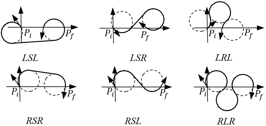
Figure 1: Types of Dubins path

Dubins pointed out that to become the optimal path, the circular arc C should be arc with the minimum radius allowed by AMR. This conclusion was later proved by Reeds and Shepp[11]. They further shortened the path by allowing reversals of motion(i.e. introducing cusps into the path). The trajectory is therefore more complex.

Although the shorter path has been studied, Dubins path still has a significance of its own in the context of robotics. For example, in many motion planning tasks, motion reversals are not feasible. The Dubins path is still a valuable reference for path planning of warehouse logistics robots.

Dubins only proved the existence of the shortest path, but not how to calculate it. To obtain the optimal Dubins path, the length of all 6 types of trajectories have to be calculated and compared, which is very computationally intensive. The scheme for fast computation of Dubins path for long distance has been solved[13], but the scheme for short distance is still unsolved. In some cases where strict real-time requirements apply, such as the study of the real-time robot motion planning[12], this may cause problems. In addition, the curvature of Dubins path is not continuous, since the path consists of line segments and circular arcs with fixed curvature. The robots have to stop to adjust the steering wheel, which reduces efficiency and increases energy consumption. Therefore, for logistics robot, Dubins path is not complete and should be improved to trajectory planning.

We first introduce, in Section II, some properties of Dubins path as a basis for the following computation. The complete computation method is then fully developed based on the angle quadrants of the corresponding pairs of the initial and final orientation angles in Section III, without explicitly computing the length of all types. In Section IV, Dubins path is turned into trajectory planning and the problem that the curvature is not continuous is solved based on clothoid. In Section V, the experimental results are presented.

II Properties of Dubins path

Dubins path is composed of three segments, where the first and the last segment are arcs. The initial and final arc segments in the Dubins path are denoted $C_{il}$, $C_{ir}$, $C_{fl}$, $C_{fr}$(where i and f stand for “initial” and “final”, and r and l stand for “right” and “left”). Then the case of intersection of union $\{C_{il}\cup C_{ir}\}$ and $\{C_{fl}\cup C_{fr}\}$, i.e. $\{C_{il}\cup C_{ir}\}\cap\{C_{fl}\cup C_{fr}\}\neq\emptyset$, is the short distance case.

II-A Model of AMR

Dubins path is for car-like vehicles. The model of AMR for Dubins path is shown in Fig. 2. and the motion equation is:

$$\dot{x} =v\cos\rho$$ (1)

$$\dot{y} =v\sin\rho$$

$$\dot{\rho} =\frac{v}{b}\tan\phi.$$

where $v$ is the velocity of AMR, $b$ is the wheelbase of AMR, $\theta$ is the angle of AMR and $\phi$ is the angle of steering wheel.

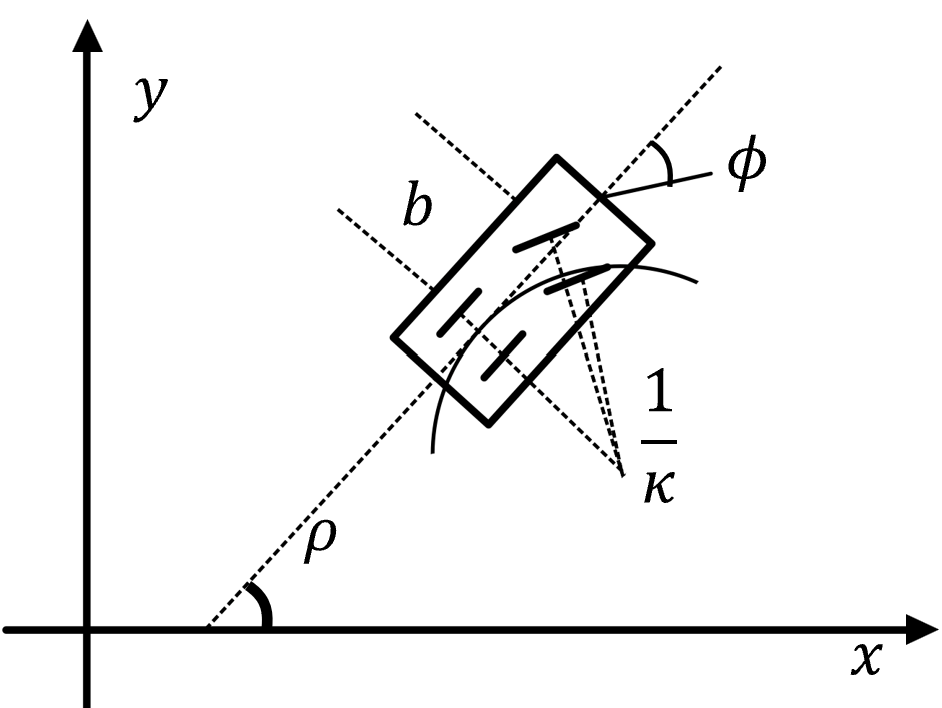
Figure 2: AMR model of Dubins path

It is easy to plan the path for AMR with four steering wheels(they can even turn in place), compared to car-like vehicles. Dubins path may not be suitable for this AMR. Regardless of the robots in operation, a smooth trajectory is still necessary, in terms of avoiding excessive acceleration of the actuators and vibrations of the mechanical structure, which is important for logistics robots. Therefore, robots that follow the trajectory developed from Dubins path can work quickly and safely.

II-B Coordinate Transformation

The first step of common method of computing Dubins path is transforming the initial point to the origin of the coordinate and final point to$x$-axis by orthogonal transformation and then normalize the radius of the arc. Denoting the initial position and orientation angle $(0,0,\alpha)$ and the final position and orientation angle $(d,0,\beta)$, as shown in Fig. 3. Then it is easy to see that:

$$\alpha =\theta_{i}-\phi$$ (2)

$$\beta =\theta_{f}-\phi$$

$$d =D/r$$

$$\phi =\arctan\frac{y_{f}-y_{i}}{x_{f}-x_{i}}$$

$$D =\sqrt{(y_{f}-y_{i})^{2}-(x_{f}-x_{i})^{2}}$$

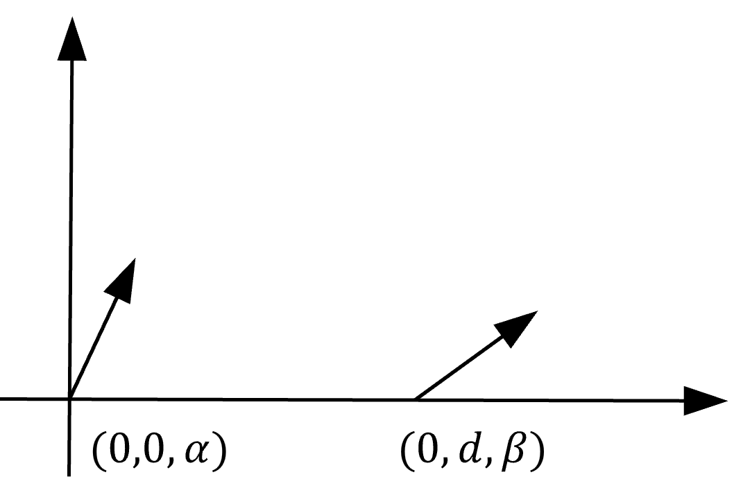
Figure 3: Position and orientation angle of initial and final point

II-C Critical Distance

As mentioned before, the condition of short distance case is $\{C_{il}\cup C_{ir}\}\cap\{C_{fl}\cup C_{fr}\}\neq\emptyset$, that is the distance between the centers of circles at initial and final points should be shorter than $2$. So the critical distance $d_{0}$ is

$$d_{0} =\max\{d_{ll},d_{lr},d_{rl},d_{rr}\}$$ (3)

$$d_{ll} =\sqrt{4-(\cos\alpha-\cos\beta)^{2}-\sin\alpha+\sin\beta}$$

$$d_{lr} =\sqrt{4-(\cos\alpha+\cos\beta)^{2}-\sin\alpha-\sin\beta}$$

$$d_{rl} =\sqrt{4-(\cos\alpha+\cos\beta)^{2}+\sin\alpha+\sin\beta}$$

$$d_{rr} =\sqrt{4-(-\cos\alpha+\cos\beta)^{2}+\sin\alpha-\sin\beta}$$

where $d_{ll}$ is the horizontal distance of the centers of the counterclockwise circle at initial point and the counterclockwise circle at final point, as the line segment $AB$ shown in Fig. 4, and so on.

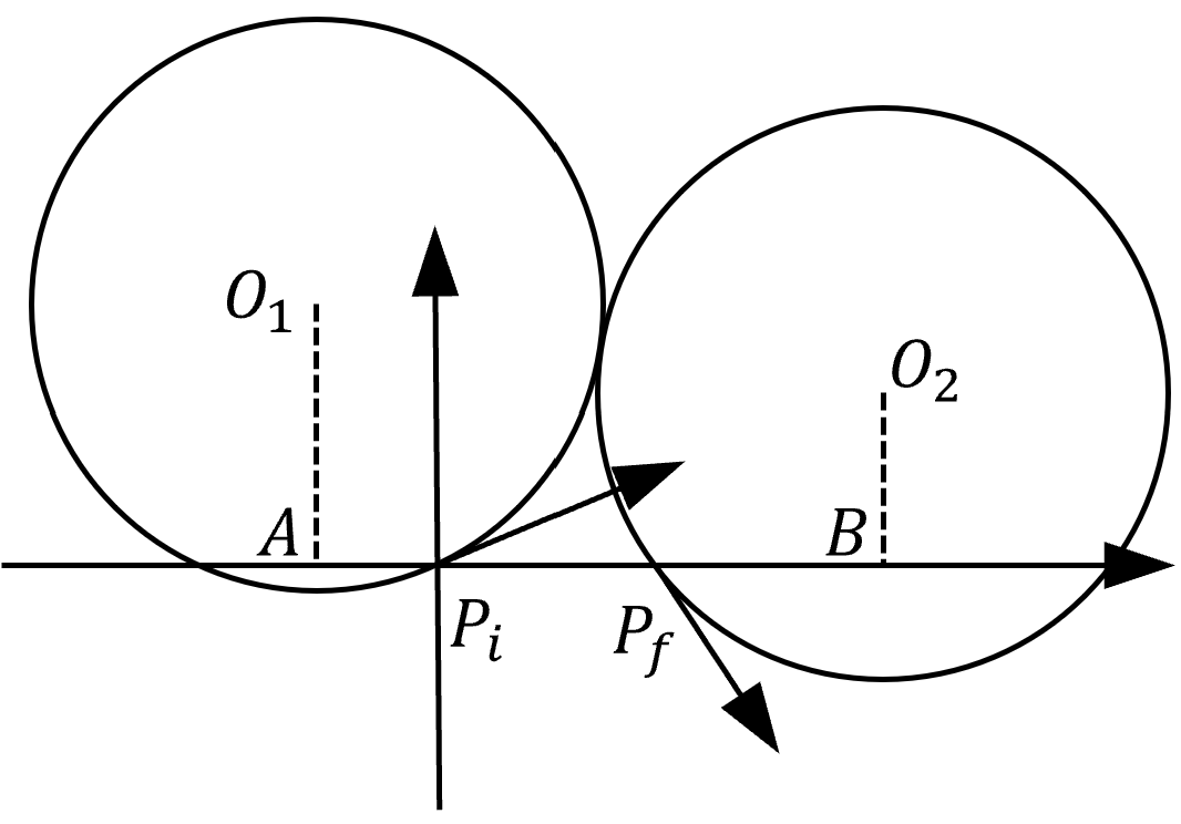
Figure 4: Line segment $d_{ll}$

Compared with long distance case, CCC may be optimal and some trajectories may not exist, e.g. when $C_{ir}\cap C_{fl}\neq\emptyset$, RSL doesn’t exist.

II-D Path Equivalency Groups

After coordinate transformation, divide the range of possible orientation angles $(\alpha,\beta)$ into four quadrants: quadrant 1 corresponds to the range $[0,\pi/2)$, quadrant 2 to $[\pi/2,\pi)$, quadrant 3 to $[\pi,3\pi/2)$, and quadrant 4 to the range $[3\pi/2,2\pi)$. Since each of $\alpha$ or $\beta$ can be in any of the four quadrants, together this produces $16$ different combinations of possible quadrants. We represent each of them by element $a_{ij}$, where index $i$ corresponds to the quadrant number of the initial, and $j$ that of the final orientation. For example, the case $\alpha\in[0,\pi/2)$, $\beta\in[3\pi/2,2\pi)$ corresponds to $a_{12}$. Actually, those $a_{ij}$ can be divided into six independent cluster, called equivalency groups[13]: $\mathbb{E}_{1}=\{a_{11},a_{44}\}$, $\mathbb{E}_{2}=\{a_{12},a_{21},a_{34},a_{43}\}$, $\mathbb{E}_{3}=\{a_{13},a_{31},a_{24},a_{42}\}$, $\mathbb{E}_{4}=\{a_{14},a_{41}\}$, $\mathbb{E}_{5}=\{a_{22},a_{33}\}$, $\mathbb{E}_{6}=\{a_{23},a_{32}\}$.

Elements in the same group have similar optimal trajectories, which greatly reduces the computation. After an optimal path of an element is computed, that of other classes in the same equivalency group can be obtained by orthogonal transformation.

II-E The Necessary Condition of Path of Type CCC Being Optimal Path

Since CCC may be the optimal path in short distance case, it is necessary to analyse its property.

The first and third segments that make up the path of type CCC are two arcs with the same orientation. The second segment should be an arc with the opposite orientation and is tangent to the two arcs. Actually, there are two arcs meeting the condition, so there are two possible trajectories, as shown by the solid line in Fig. 5. Therefore, it is important to know which is the optimal path.

Figure 5: Two possible CCC path

Theorem 1

The necessary condition of path of type CCC being optimal trajectory is:1)the initial and final points are on the opposite sides of the rhombus and $\varphi<\pi/2$, or 2)they are on the same side of the rhombus.

Proof:

As shown in Fig. 5, the lines connecting the centers of four circles make up a rhombus. If the initial and final points, $P_{i}$ and $P_{f}$, are both on the inside or outside of the rhombus, they are considered to be on the same side; otherwise they are considered to be on the opposite side. Let $c_{1}$ and $c_{2}$ denote the length of path in 5, respectively.

Consider the case when initial and final points are in the same side first. If they are both on the inside, as shown in Fig. 6(a),the length of two trajectories are

$$c_{1}=\varepsilon_{1}+(\alpha+\pi)+\varepsilon_{2}$$ (4)

$$c_{2}=[2\pi+(\alpha-\varepsilon_{1})]+(\pi-\alpha)+(2\pi-\alpha+\varepsilon_{2})$$

$$c_{2}-c_{1}=4(\pi-\alpha)>0.$$

Similarly, if they are both on the outside, as shown in Fig. 6(b), the difference of the length is

$$c_{2}-c_{1}=-4\varphi<0.$$ (5)

Therefore, if initial and final points are both on inside, the optimal path cannot be the path where the middle arc is a inferior arc(for the other is shorter). When they are both on outside, the optimal path cannot be the path where the middle arc is a superior arc.

(a) Both on the inside

(b) Both on the outside

Figure 6: Initial and final points are on the same side

When they are on the opposite side, the difference of path length is

$$c_{2}-c_{1}=4(\frac{\pi}{2}-\varphi).$$ (6)

Therefore, when $\varphi>\pi/2$, the optimal path cannot be the path where the middle arc is a superior arc and when $\varphi<\pi/2$, the optimal path cannot be the other one.

Actually, no path of type CCC, where the middle arc is of length not greater than $\pi R$, can be an optimal path[14]. So a path of type CCC cannot be an optimal path when the initial and final points are on the opposite side and $\varphi<\pi/2$ or they are both on outside.

∎

III Complete Computation Method of Dubins path

The calculation of the Dubins path for long distances has been solved[13], while that for short distances has not yet been studied. Therefore, in this section, the scheme for calculating the Dubins path for short distances will be fully developed. Then, an auxiliary method to simplify the calculation is presented.

The following additional notation is used below: unless stated otherwise, forms suck as $AB$ and $\wideparen{AB}$ represent straight line segments and circular arc segments, respectively, with A and B being the segments’ endpoints. When needed for clarity, the strings may be longer: e.g. $A_{1}\wideparen{B_{1}C_{1}}D_{1}$ is an arc with the endpoints $A_{1}$, $D_{1}$ and two inner points $B_{1}$, $C_{1}$. Let $d$ and its subscript denote the horizontal distance of centers of circles at initial and final positions, and the subscript denote the orientation of the circle. $d_{ll}$ is e.g. the horizontal distance of the centers of the counterclockwise circle at initial position and the counterclockwise circle at final position, i.e., the line segment $AB$ in Fig. 4. Let $t$, $p$ and $q$ denote the length of the first, second and third segments of path, respectively, and the subscript denote the type of path, e.g., $t_{lsl}$ is the length of the first segment of path of type LSL. Let $\mathcal{L}$ and its subscript denote the length of path .The computation method can be found in [13].

III-A Equivalency Group $\mathbb{E}_{1}$

As mentioned in Section II-D, classes $a_{11}$ and $a_{44}$ belong to the same equivalency group. We first show for class $a_{11}$ how to compute optimal path. Then by applying an orthogonal transformation to the optimal path for class $a_{11}$, the optimal solution for $a_{44}$ will be obtained.

Theorem 2

For the short distance case, the optimal path corresponding to the class $a_{11}$ may be LSL, RSR, RSL, LSR, RLR, LRL, and is shown in Tab . I.

TABLE I: Optimal Path Corresponding to Class $a_{11}$

Condition			Optimal Path
$d_{rl}<d<d_{0}$			RSL
$d<d_{rl}$	$\alpha<\beta$	$t_{rsr}<\pi,S_{11}^{1}>0$	RSR
		$t_{rsr}>\pi,S_{11}^{2}>0$	LSR
		Otherwise	RLR
	$\alpha>\beta$	$q_{lsl}<\pi,S_{11}^{3}>0$	LSL
		$q_{lsl}>\pi,S_{11}^{4}>0$	LSR
		Otherwise	LRL

the switching functions in Tab. I are

$$S_{11}^{1} =2(p_{rlr}-\pi)-p_{rsr},$$ (7)

$$S_{11}^{2} =2(t_{rlr}+q_{rlr})-(p_{lsr}+2q_{lsr})+2\pi,$$

$$S_{11}^{3} =2(p_{lrl}-\pi)-p_{lsl},$$

$$S_{11}^{4} =2(t_{lrl}+q_{lrl})-(p_{lsr}+2t_{lsr})+2\pi.$$

Proof:

Since $\mathcal{L}_{rsl}<\min\{\mathcal{L}_{lsl},\mathcal{L}_{rsr},\mathcal{L}_{lsr}\}$[13], when RSL path exists, the optimal path is RSL, i.e.

$$d_{rl}<d<d_{0}$$ (8)

It is easy to see that $\mathcal{L}_{lsl}=\mathcal{L}_{rsr}$, $\mathcal{L}_{lrl}=\mathcal{L}_{rlr}$ when $\alpha=\beta$. Furthermore, $\frac{\partial\mathcal{L}_{lsl}}{\partial\alpha}<0$, $\frac{\partial\mathcal{L}_{lsl}}{\partial\beta}>0$; $\frac{\partial\mathcal{L}_{rsr}}{\partial\alpha}>0$, $\frac{\partial\mathcal{L}_{rsr}}{\partial\beta}<0$. Therefore, $\mathcal{L}_{rsr}<\mathcal{L}_{lsl}$, $\mathcal{L}_{rlr}<\mathcal{L}_{lrl}$ when $\alpha<\beta$; $\mathcal{L}_{rsr}>\mathcal{L}_{lsl}$, $\mathcal{L}_{rlr}>\mathcal{L}_{lrl}$ when $\alpha>\beta$.

We should consider the relationship between RLR, RSR and LSR when $\alpha<\beta$.

We first compute the switching function between RSR and LSR. Define the critical initial orientation as one where orientation $\alpha$ coincides with the tangent to the circle $O_{fr}$, as shown in Fig. 7.; denote it $\alpha=\overline{\alpha}$. $\overline{\alpha}$ is uniquely defined by the set $(\beta,d)$. $P_{i}\wideparen{TP_{f}}$ is their degenerate path SR, which implies that if $\alpha>\overline{\alpha}$ then path LSR can be excluded from consideration($\mathcal{L}_{lsr}>\mathcal{L}_{rsr}$); conversely path RSR can be excluded. Actually, if $\alpha>\overline{\alpha}$ then $t_{lsr}>\pi$ and $t_{rsr}<\pi$; conversely $t_{lsr}<\pi$ and $t_{rsr}>\pi$. So $t_{rsr}$(or $t_{lsr}$) can be the switching function. If $t_{rsr}>\pi$ then $\mathcal{L}_{rsr}>\mathcal{L}_{lsr}$; if $t_{rsr}<\pi$ then $\mathcal{L}_{rsr}<\mathcal{L}_{lsr}$.

Figure 7: Critical initial orientation

The computation of switching function between RLR and RSR is more complex. As shown in Fig. 8, $\wideparen{P_{i}A}\wideparen{BP_{f}}$ is RSR path and $\wideparen{P_{i}DEP_{f}}$ is RLR path. $O_{tl}$ is the common tangent circle of $O_{ir}$ and $O_{fr}$, $AO_{ir}//CO_{tl}//BO_{fr}$, $FP_{f}//GH$. So $\mathcal{L}_{rlr}$, $\mathcal{L}_{rsr}$ and the switching function $S_{11}^{1}$ respectively are

$$\mathcal{L}_{rlr} =(\xi+\gamma)+[(\gamma-\zeta)+\pi+\sigma]+\sigma$$ (9)

$$\mathcal{L}_{rsr} =\xi+p_{rsr}+\zeta+\pi$$

$$S_{11}^{1} =\mathcal{L}_{rlr}-\mathcal{L}_{rsr}=2(p_{rlr}-\pi)-p_{rsr}$$

If $S_{11}^{1}>0$ then $\mathcal{L}_{rlr}>\mathcal{L}_{rsr}$; conversely $\mathcal{L}_{rlr}<\mathcal{L}_{rsr}$.

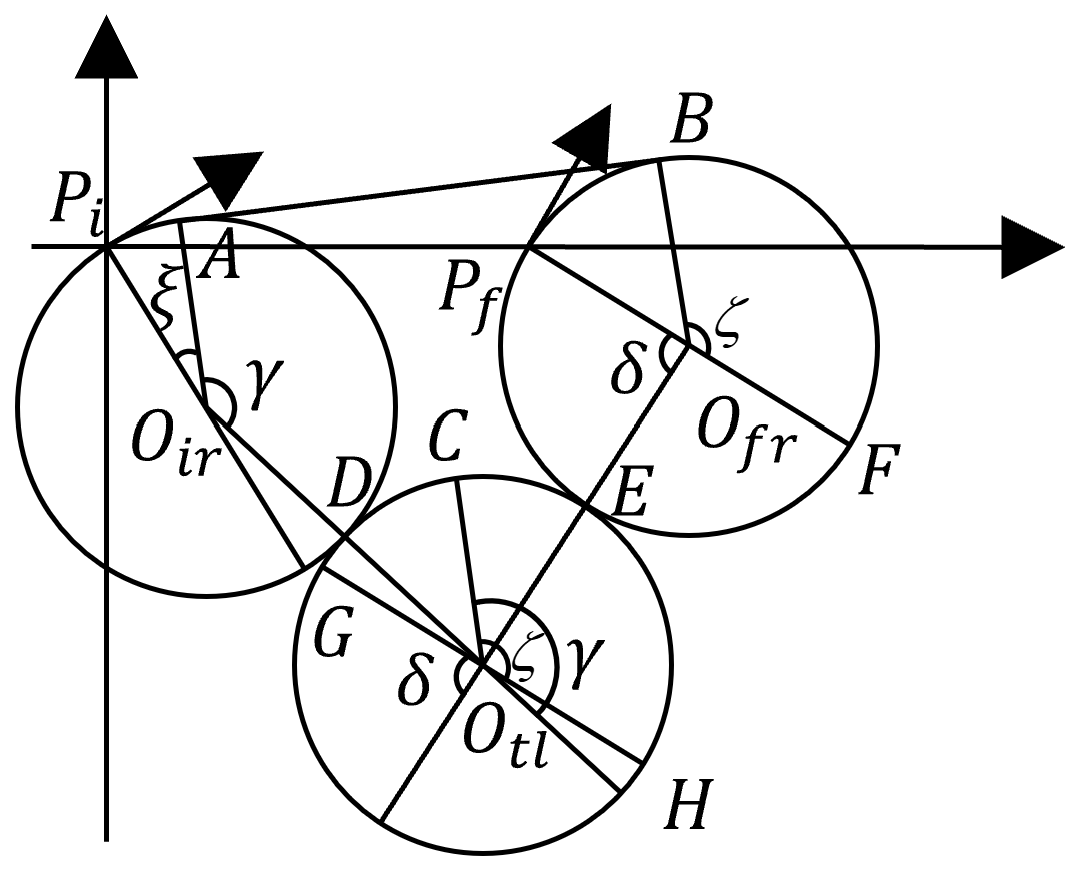
Figure 8: Computation of the switching function $S_{11}^{1}$ for class $a_{11}$

The computation of switching function between RLR and LSR is similar with that of $S_{11}^{1}$. As shown in Fig. 9, $\mathcal{L}_{rlr}$, $\mathcal{L}_{lsr}$ and the switching function $S_{11}^{2}$ respectively are

$$\mathcal{L}_{rlr} =\xi+\xi+\gamma+\zeta+\delta+\delta$$ (10)

$$\mathcal{L}_{lsr} =\gamma+p_{lsr}+2\pi-\zeta$$

$$S_{11}^{2} =\mathcal{L}_{rlr}-\mathcal{L}_{lsr}=2(t_{rlr}+q_{rlr})-(p_{lsr}+2q_{lsr})+2\pi$$

If $S_{11}^{2}>0$ then $\mathcal{L}_{rlr}>\mathcal{L}_{lsr}$; conversely $\mathcal{L}_{rlr}<\mathcal{L}_{lsr}$.

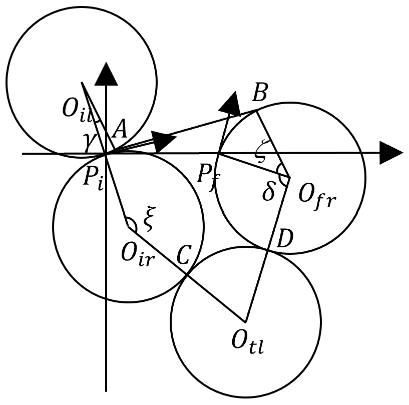
Figure 9: Computation of switching function $S_{11}^{2}$ for class $a_{11}$

We should consider the relationship between LRL, LSL and LSR when $\alpha<\beta$. Similarly, $S_{11}^{3}=2(p_{lrl}-\pi)-p_{lsl}$, $S_{11}^{4}=2(t_{lrl}+q_{lrl})-(p_{lsr}+2t_{lsr})+2\pi$.

It is noteworthy that the switching function between LSL and LSR is $q_{lsl}$, for their common degenerated path is LS. Define the critical final orientation as one where orientation $\beta$ coincides with the tangent to the circle $O_{il}$, as shown in Fig. 10.; denote it $\beta=\overline{\beta}$. $\overline{\beta}$ is uniquely defined by the set $(\alpha,d)$. LSR can be excluded from consideration if $\beta>\overline{\beta}$($\mathcal{L}_{lsr}>\mathcal{L}_{rsr}$); conversely LSR can be excluded. That’s why $t_{rsr}$ is the switching function if $\alpha<\beta$; $q_{lsl}$ is the switching function if $\alpha>\beta$.

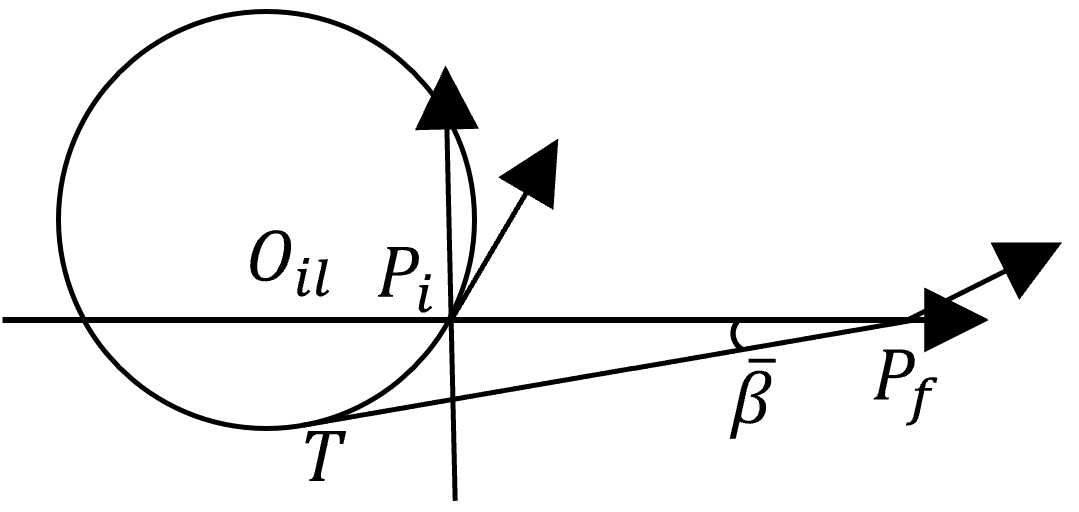
Figure 10: Critical final orientation

∎

III-B Equivalency Group $\mathbb{E}_{2}$

As mentioned in Section II-D, classes $a_{12}$, $a_{21}$, $a_{34}$ and $a_{43}$ belong to the same equivalency group. We first show for class $a_{12}$ how to compute optimal path, then by applying an orthogonal transformation to the optimal path for class $a_{12}$, the optimal solution for other classes will be obtained.

Theorem 3

For the short distance case, the optimal path corresponding to the class $a_{12}$ may be RSR, LSR, RLR, LRL.

Proof:

It is easy to see that $C_{ir}\cap C_{fl}\neq\emptyset$ does occur for short distance case, so path RSL is not feasible and can be excluded from consideration. For short distance case, as shown in Fig. 11,the length of first segment of LSL is greater than $\pi$, so $\mathcal{L}_{lsl}>|P_{i}\wideparen{TP_{f}}|$, which implies that $\mathcal{L}_{lsr}<\mathcal{L}_{lsl}$ if $\alpha<\overline{\alpha}$; $\mathcal{L}_{lsr}>\mathcal{L}_{lsl}$ if $\alpha>\overline{\alpha}$. Therefore, type LSL can be excluded as well.

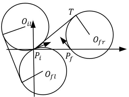
Figure 11: LSL cannot be the optimal path for class $a_{12}$

∎

Theorem 4

For the short distance case, the optimal path corresponding to the class $a_{12}$ is shown in Tab. II.

TABLE II: Optimal Path Corresponding to Class $a_{12}$

Condition			Optimal Path
$d_{lr}<d<d_{0}$	$t_{rsr}<\pi$	$S_{12}^{1}<0$	RLR
		$S_{12}^{1}>0$	RSR
	$t_{rsr}>\pi$	$S_{12}^{2}<0$	RLR
		$S_{12}^{2}>0$	LSR
$d<d_{lr}$			LRL

the switching functions in Tab. II are

$$S_{12}^{1} =2(p_{rlr}-\pi)-p_{rsr},$$ (11)

$$S_{12}^{2} =2(t_{rlr}+q_{rlr})-(p_{lsr}+2q_{lsr})+2\pi.$$

Proof:

The possible optimal trajectories are RLR, RSR and LSR if $C_{il}$ and $C_{fr}$ do not intersect. Similar to $a_{11}$, $t_{rsr}$(or $t_{lsr}$) can be the switching function between RSR and LSR with $\overline{\alpha}$ being the critical initial orientation. Then compare the length of them with that of RLR, respectively.

If the four circle intersect with each other, i.e. $d<d_{lr}$, path LSR does not exist . The length of first and third segments of RSR are both greater than $\pi$, which makes the length of RSR much greater than that of others. Therefore it is impossible for trajectories of type of CSC to be optimal path. Furthermore, $\mathcal{L}_{rlr}-\mathcal{L}_{lrl}>0$, so the optimal path is LRL. ∎

The respective switching functions for classes $a_{21}$, $a_{34}$, and $a_{43}$ are obtained from the switching function for class $a_{12}$.

III-C Equivalency Group $\mathbb{E}_{3}$

According to section II-D, classes $a_{13}$, $a_{31}$, $a_{24}$ and $a_{42}$ belong to the same equivalency group. We first show for class $a_{13}$ how to compute optimal path, then by applying an orthogonal transformation to the optimal path for class $a_{13}$, the optimal solution for other classes will be obtained.

Theorem 5

For the short distance case, the optimal path corresponding to the class $a_{13}$ may be RSR, RSL, LSR, RLR and LRL, and is shown in Tab. III.

TABLE III: Optimal Path Corresponding to Class $a_{13}$

Condition			Optimal Path
$d<d_{lr}$	$d<d_{rl}$	$S_{13}^{1}<0$	RLR
		$S_{13}^{1}>0$	LRL
	$d>d_{rl}$	$S_{13}^{2}<0$	LRL
		$S_{13}^{2}>0$	RSL
$d>d_{lr}$	$t_{rsr}<\pi$		RSR
	$t_{rsr}>\pi$		LSR

the switching functions in Tab. III are

$$S_{13}^{1} =\alpha-\beta+p_{rlr}-p_{lrl},$$ (12)

$$S_{13}^{2} =2(q_{lrl}+t_{lrl})+2q_{rsl}-p_{rsl}-2\pi.$$

Proof:

For case of class $a_{13}$(i.e. $\alpha\in[0,\pi/2)$, $\beta\in[\pi,3\pi/2)$), the distance between $C_{il}$ and $C_{fl}$ is greater than that between $C_{ir}$ and $C_{fr}$. We may think that inequality $\mathcal{L}_{lsl}>\mathcal{L}_{rsr}$ may hold. Actually, if $\alpha=0,\beta=\pi$ then $\mathcal{L}_{lsl}=\mathcal{L}_{rsr}$, so if $\alpha>0,\beta>\pi$ then $\mathcal{L}_{lsl}>\mathcal{L}_{rsr}$. Hence LSL can be excluded from the list of candidates for an optimal solution.

Similar to the long distance case, if path of type of LSR or RSR exist(i.e. $C_{il}\cap C_{fr}=\emptyset$), the optimal path is one of them, and so the switching function.

When $C_{il}\cap C_{fr}\neq\emptyset$, whether $C_{ir}$ and $C_{fl}$ intersect have an effect on the optimal path. If they are tangent then $\mathcal{L}_{rsl}=\mathcal{L}_{rlr}$(the path is their common degenerated curve $RL$, actually). Accordingly, if $C_{ir}\cap C_{fl}=\emptyset$ then $\mathcal{L}_{rsl}<\mathcal{L}_{rlr}$. Similarly, RSR can be excluded from consideration. There are still RSL and LRL left. As shown in Fig. 12, the length of them and the switching function $S_{13}^{2}$ respectively are

$$\mathcal{L}_{lrl} =2\gamma+\xi+\delta+2\zeta$$ (13)

$$\mathcal{L}_{rsl} =\xi+p_{rsl}+2\pi-\zeta$$

$$S_{13}^{2} =\mathcal{L}_{lrl}-\mathcal{L}_{rsl}$$

$$=2(t_{lrl}+q_{lrl})+2q_{rsl}-p_{rsl}-2\pi$$

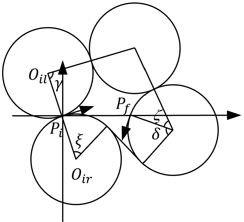
Figure 12: Computation of switching function $S_{13}^{2}$ for class $a_{13}$

RSL does not exist if $C_{ir}\cap C_{fl}\neq\emptyset$, so now only need to compare $\mathcal{L}_{lrl}$ and $\mathcal{L}_{rlr}$. The switching function is

$$S_{13}^{1} =\frac{\mathcal{L}_{rlr}-\mathcal{L}_{lrl}}{2}$$ (14)

$$=\alpha-\beta+p_{rlr}-p_{lrl}$$

∎

It is easy to obtain optimal trajectories of other classes in $\mathbb{E}_{3}$ by applying orthogonal transformation.

III-D Equivalency Group $\mathbb{E}_{4}$

Classes $a_{14}$, $a_{41}$ belong to the same equivalency group. We first show for class $a_{14}$ how to compute optimal path, then by applying an orthogonal transformation to the optimal path for it, the optimal solution for the other will be obtained.

Theorem 6

For the short distance case, the optimal path corresponding to the class $a_{14}$ may be RSR, RSL, LSR, RLR and LRL, and is shown in Tab. IV.

TABLE IV: Optimal Path Corresponding to Class $a_{14}$

Condition		Optimal Path
$d_{lr},d_{rl}<d<d_{0}$	$t_{rsr}>\pi$	LSR
	$q_{rsr}>\pi$	RSL
	Otherwise	RSR
$d_{rl}<d<d_{lr}$	$S_{14}^{1}<0$	LRL
	$S_{14}^{1}>0$	LSR
$d_{lr}<d<d_{rl}$	$S_{14}^{2}<0$	LRL
	$S_{14}^{2}>0$	RSL
$d<d_{lr},d_{rl}$	$S_{14}^{3}<0$	RLR
	$S_{14}^{3}>0$	LRL

the switching functions in Tab. IV are

$$S_{14}^{1} =2(t_{lrl}+q_{lrl})+2t_{lsr}-p_{lsr}-2\pi,$$ (15)

$$S_{14}^{2} =2(t_{lrl}+q_{lrl})+2q_{rsl}-p_{rsl}-2\pi,$$

$$S_{14}^{3} =\alpha-\beta+p_{rlr}-p_{lrl}.$$

Proof:

For class $a_{14}$, $C_{ir}$ and $C_{fr}$ will intersect first. The optimal solution in this case is similar to that in long distance case. There are two cases if the initial and final positions get closer: $C_{il}$ and $C_{fr}$ intersect first(i.e. $d_{rl}<d<d_{lr}$) or $C_{ir}$ and $C_{fl}$ intersect first(i.e. $d_{lr}<d<d_{rl}$), as shown in Fig. 13.

Consider the case that $C_{il}$ and $C_{fr}$ intersect first. It is easy to see that $P_{i}$ and $P_{f}$ are on the outside of the rhombus for $C_{ir}$ and $C_{fr}$. According to theorem 1, RLR cannot be optimal path. The length of the first and third segments of LSL are both greater than $\pi$, which leads to $\mathcal{L}_{lsl}\gg\mathcal{L}_{lsr}$ and similarly $\mathcal{L}_{rsr}>\mathcal{L}_{lsr}$. Hence, LSL and RSR can be excluded from list of candidates for an optimal solution and the possible optimal trajectories are LRL and LSR. Similarly, if $C_{ir}$ and $C_{fl}$ intersect first, the possible optimal trajectories may be LRL and RSL .

Furthermore, if $d<d_{lr},d_{rl}$, LSR and RSL do not exist and the length of RSR and LSL are both greater than that of type CCC. Accordingly, the type of optimal path should be CCC. As for the switching functions, the computation is the same as described in the previous section.

Figure 13: Case that $C_{il}$ and $C_{fr}$ intersect first(left) and case that $C_{ir}$ and $C_{fl}$ intersect first(right)

∎

By applying the orthogonal transformation to the path of class $a_{14}$, the optimal solution for class $a_{41}$ will be obtained.

III-E Equivalency Group $\mathbb{E}_{5}$

According to section II-D, classes $a_{22}$ and $a_{33}$ belong to equivalency group $\mathbb{E}_{5}$. We first show for class $a_{22}$ how to compute optimal path, then by applying an orthogonal transformation to the optimal path for it, the optimal solution for $a_{33}$ will be obtained.

Theorem 7

For the short distance case, the optimal path corresponding to the class $a_{22}$ may be RSR, LSL, LSR, RLR and LRL, and is shown in Tab. V.

TABLE V: Optimal Path Corresponding to Class $a_{22}$

Condition		Optimal Path
$\alpha<\beta$	$q_{lsl}>\pi$	LSR
	$q_{lsl}<\pi,S_{22}^{1}>0$	RSR
	$q_{lsl}<\pi,S_{22}^{1}<0$	RLR
$\alpha>\beta$	$t_{rsr}>\pi$	LSR
	$t_{rsr}<\pi,S_{22}^{2}>0$	LSL
	$t_{rsr}<\pi,S_{22}^{2}<0$	LRL

the switching functions in Tab. V are

$$S_{22}^{1} =2(p_{rlr}-\pi)-p_{rsr},$$ (16)

$$S_{22}^{2} =2(p_{lrl}-\pi)-p_{lsl}.$$

Proof:

Similar to class $a_{11}$, $\mathcal{L}_{rsr}=\mathcal{L}_{lsl}$, $\mathcal{L}_{rlr}=\mathcal{L}_{lrl}$ holds, if $\alpha=\beta$. Hence, the comparison between $\mathcal{L}_{rsr}$ and $\mathcal{L}_{rlr}$ and that between $\mathcal{L}_{lsl}$ and $\mathcal{L}_{lrl}$ can refer to the class $a_{11}$.

The calculation of switching functions between LSR and RSR and that between LSR and LSL may also refer to the class $a_{11}$. Let $\overline{\alpha}$ and $\overline{\beta}$ be the critical orientation, i.e. let $t_{rsr}$ and $q_{lsl}$ be the switching functions. The difference is that when $\alpha<\beta$, to achieve $\mathcal{L}_{lsr}<\mathcal{L}_{rsr}$, i.e. $t_{rsr}>\pi$, $P_{f}$ should be close to $P_{i}$ and the angle $\varphi$ should be greater than $\frac{\pi}{2}$, which means that $P_{i}$ and $P_{f}$ are on the opposite side of the rhombus. According to theorem 1, RLR is impossible to be the optimal path. Similarly, when $\alpha>\beta$, if $q_{lsl}>\pi$, LRL cannot be the optimal path.

∎

By applying orthogonal transformation, the optimal solution for class $a_{33}$ is easy to obtained.

III-F Equivalency Group $\mathbb{E}_{6}$

Classes $a_{23}$ and $a_{32}$ belong to equivalency group $\mathbb{E}_{6}$. We first show for class $a_{23}$ how to compute optimal path, then by applying an orthogonal transformation to the optimal path for it, the optimal solution for $a_{32}$ will be obtained.

Theorem 8

For the short distance case, the optimal path corresponding to the class $a_{23}$ may be RSR, RSL, LSR and LRL, and is shown in Tab. VI.

TABLE VI: Optimal Path Corresponding to Class $a_{23}$

Condition		Optimal Path
$d_{lr},d_{rl}<d<d_{0}$		RSR
$d_{rl}<d<d_{lr}$	$q_{rsr}<0$	RSR
	$q_{rsr}>0$	RSL
$d_{lr}<d<d_{rl}$	$t_{rsr}<0$	RSR
	$t_{rsr}>0$	LSR
$d<d_{lr},d_{rl}$		LRL

Proof:

Trajectories of types LSL and RLR are excluded from consideration for class $a_{23}$. Since $\mathcal{L}_{rsr}<\mathcal{L}_{lsl}$ holds[13], LSL also cannot be the optimal path. Furthermore, $P_{i}$ and $P_{f}$ are both the outside of the rhombus in path of type RLR. According to theorem 1, RLR is impossible to be the optimal path.

For class $a_{32}$, $C_{ir}$ and $C_{fl}$ intersect first. When only these two circles intersect, the conclusion of the long distance case still applies, so the optimal path is RSR in this case.

If the distance between the initial and final positions is relatively far, $\alpha>\overline{\alpha}$ and $\beta<\overline{\beta}$ hold, but may not necessarily do if the distance is close. If $P_{i}$ and $P_{f}$ get closer, there are two cases: 1. $C_{il}$ and $C_{fr}$ intersect first; 2. $C_{ir}$ and $C_{fl}$ intersect first. For case 1, let $\overline{\beta}$ be the critical final orientation. If $\beta>\overline{\beta}$, $\mathcal{L}_{rsr}>\mathcal{L}_{rsl}$ holds; if $\beta<\overline{\beta}$, $\mathcal{L}_{rsr}<\mathcal{L}_{rsl}$ holds. For case 2, let $\overline{\alpha}$ be the critical initial orientation. If $\alpha>\overline{\alpha}$, $\mathcal{L}_{lsr}>\mathcal{L}_{rsr}$ holds; if $\alpha<\overline{\alpha}$, $\mathcal{L}_{lsr}<\mathcal{L}_{rsr}$ holds.

Trajectories of types LSR and RSL do not exist if the four circles intersect with each other. Since $C_{fr}$ is on the left of $C_{ir}$, the length of the first and third segments of RSR are both greater than $\pi$, so RSR cannot be the optimal path. Therefore, the optimal path can only be LRL. ∎

IV From Dubins Path to Trajectory

Dubins path meets the kinematic constraints of the AMR and the AMR can follow the path. However, since the path is composed of line segments and arcs with curvature equal to the maximum steering curvature of the AMR, the curvature of the path is not continuous and there are abrupt changes in curvature at the junction of line segments and arcs. AMR moving to the junction needs to stop and adjust the steering wheels to the maximum angle before proceeding. Therefore, it is necessary to smooth the curve to make it more suitable for AMR movement.

IV-A Continuous Curvature Turn

Clothoid, whose curvature varies linearly with its arc length, is defined by Fresnel integral. The differential equation of it is

$$\mathrm{d}\kappa=\sigma\mathrm{d}l$$ (17)

where $\kappa$ is the curvature of the curve, $l$ is the length of the curve and $\sigma$, relating to the steering velocity of the front wheels, is the sharpness of the clothoid.

Clothoid is often used in trajectory or path planning[15, 16, 17, 18] and the discontinuity can be well solved by the clothoid.It is used to connect the straight-line segments to the circular arc segments and is drivable because the steering wheel turns in a continuous motion[19].The steering velocity is described by sharpness $\sigma$, the greater the sharpness is, the faster the velocity. In other words, $\sigma$ is the upper-bounded curvature derivative. The turns of the trajectory smoothed by the clothoid should be symmetrical, for the AMR adjusts its steering wheels at a constant velocity and there are straight-lines outside the turns. Therefore, The second half of the turn can be obtained symmetrically by the first half of that.

Before smoothing the trajectory, it is necessary to distinguish between different types of turns. For turns with larger angles, the steering wheels turn to the maximum angle during the steering process, but for turns with smaller angles, the wheels do not turn to the maximum angle. We denote the former one sharp turn and the latter one wide turn, as shown in Fig. 14. In the sharp turn, the entry and exit points are on the same circle[20], but the wide turn does not have this property. It is therefore necessary to distinguish between the sharp turn and wide turn and to make the entry and exit points of wide on the same circle.

Figure 14: Sharp turn(left) and wide turn(right)

Theorem 9

The critical angle of sharp turn and wide turn, denoted by $\theta_{c}$, is

$$\theta_{c}=\frac{1}{2\sigma_{max}^{2}r^{2}}$$ (18)

where $\sigma_{max}$ and $r$ are the maximum steering sharpness and the minimum steering radius allowed by AMR, respectively.

Proof:

Distinguishing between sharp turn and wide turn is all about determining the critical steering angle. The parametric equation of (17) is

$$x =\frac{1}{\sigma_{max}}\int_{0}^{t}\cos(\tau^{2})\mathrm{d}\tau$$ (19)

$$y =\frac{1}{\sigma_{max}}\int_{0}^{t}\sin(\tau^{2})\mathrm{d}\tau.$$

The sharpness $\sigma$ is the only parameter of the clothoid, and if it remains constant, the clothoid is also uniquely determined. The difference between sharp and wide turns is whether the curvature of the trajectory reaches the maximum curvature, we therefore focus on the curvature of the trajectory. The curvature of the clothoid at any point $t$ is

$$\kappa=\frac{\left|\dot{x}\ddot{y}-\dot{y}\ddot{x}\right|}{[\dot{x}^{2}+\dot{y}^{2}]^{3/2}}=2\sigma_{max}t.$$ (20)

Let $t_{c}$ denote the parameter $t$ that curvature of the clothoid just reaches the maximum curvature, denoted by $\kappa_{max}$. It is easy to see that $\kappa_{max}=1/r$, so $t_{c}$ is

$$t_{c}=\frac{1}{2\sigma_{max}r}.$$ (21)

The coordinate of the tangency point $P$ can be obtained by substituting $t_{c}$ into (19), as shown in Fig. 15, i.e.

$$x_{P}=\frac{1}{\sigma_{max}}\int^{t_{c}}_{0}\cos(\tau^{2})\mathrm{d}\tau$$ (22)

$$y_{P}=\frac{1}{\sigma_{max}}\int^{t_{c}}_{0}\sin(\tau^{2})\mathrm{d}\tau.$$ (23)

Fig. 15 is the turn in the critical case. The small solid circle $O$ is the circle of maximum curvature tangent to the clothoid at the point $P$, i.e. AMR following the clothoid just adjusts the steering wheels to the maximum angle at the point $P$.

Let $\eta$ denote the angle between the tangent at point $P$ and the $x$-axis and $\theta_{out}$ denote the angle between the tangent at exit point $P_{out}$(the symmetrical point of entry point $P_{in}$ about line $OP$) and $x$-axis. It is not difficult to see that the tangents $P_{in}T$ and $P_{out}T$ are also symmetrical about line $OP$, so that the angle $\eta$ is half of $\theta_{out}$.

Note that slope of any tangent on the clothoid $k$ is

$$k=\frac{\mathrm{d}y}{\mathrm{d}x}=\tan t^{2}.$$ (24)

Accordingly, the angle between any tangent on the clothoid and $x$-axis is the square of parameter $t$. Since the case shown in Fig. 15 is the critical case, the exit angle is the critical angle, i.e. $\theta_{out}=\theta_{c}$. Hence, the critical angle $\theta_{c}$ is

$$\eta =t_{c}^{2}$$ (25)

$$\theta_{out} =2\eta$$

So the critical angle $\theta_{c}$ can be obtained from (21) and (25)

$$\theta_{c}=\frac{1}{2\sigma_{max}^{2}r^{2}}$$ (26)

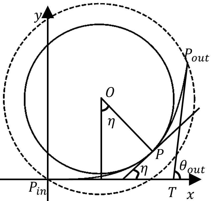
Figure 15: Critical angle

∎

Theorem 10

In critical case, the expression for the axis of symmetry of the turn in the continuous curvature trajectory is

$$Ax+By+C=0$$ (27)

$$A=\tan t_{c}^{2}$$

$$B=-1$$

$$C=y_{P}+r\cos t_{c}^{2}+A(x_{P}-r\sin t_{c}^{2})$$

where $t_{c}$ is the critical parameter and given by (21); $(x_{P},y_{P})$ is the coordinate of tangent point $P$ and given by (22).

Proof:

As mentioned earlier, the turn of the trajectory is symmetrical and the second half can obtained symmetrically by the first half. It is easy to see that the point $P$ is also the midpoint of the turn. Obviously, the axis of symmetry, i.e. line $OP$ in Fig. 15, should pass through point $P$ and be perpendicular to the tangent at point $P$. Accordingly, the slope of the axis of symmetry, denoted by $k_{m}$, is

$$k_{m}=-\frac{1}{\tan t_{c}^{2}}.$$ (28)

It is easy to get from Fig. 15 the coordinate of the center of the circle $(x_{O},y_{O})$.

$$x_{O} =x_{P}-r\sin t_{c}^{2}$$ (29)

$$y_{O} =y_{P}+r\cos t_{c}^{2}.$$

So the expression of the axis of symmetry is

$$Ax+By+C=0$$ (30)

$$A=k_{m}$$

$$B=-1$$

$$C=y_{O}+k_{m}x_{O}.$$

Additionally, any point at the second half $(x_{l},y_{l})$ is

$$x_{l}=x_{f}-2A\frac{Ax_{f}+By_{f}+C}{A^{2}+B^{2}}$$ (31)

$$y_{l}=y_{f}-2B\frac{Ax_{f}+By_{f}+C}{A^{2}+B^{2}}$$

where $(x_{f},y_{f})$ is the symmetrical point of point $(x_{l},y_{l})$ at the first half; $A$, $B$ and $C$ are the line parameter of the axis of symmetry, respectively.

By the axis of symmetry, the second half of the turn can be easily obtained by the first half. ∎

Theorem 11

The sharpness in wide turn ,denoted by $\sigma_{s}$, is

$$\sigma_{s} =\frac{C_{f}+S_{f}\tan\eta}{x_{O}+y_{O}\tan\eta}$$ (32)

$$\eta =\frac{\theta_{out}}{2}$$

where $(x_{O},y_{O})$ is the coordinate of the center of the circle and given by (29); $C_{f}$ and $S_{f}$ are the Fresnel integral; $\eta$, half of $\theta_{out}$, is the angle between the tangent at the midpoint of the turn and the $x$-axis; $\theta_{out}$ is the exit angle.

Proof:

In the sharp turn case, the steering wheels should be adjusted as quickly as possible to pass the turn quickly. Thus, the sharpness of the clothoid should be $\sigma_{max}$, the maximum sharpness allowed by the AMR. However, in the case of wide turn, the sharpness should be less. Let $P$ denote the midpoint of the turn and $\eta$ denote the angle between the tangent at $P$ and the $x$-axis. The angle $\eta$ is, obviously, half of the exit angle $\theta_{out}$, since the turn is symmetrical. The slope of the tangent, denoted by $k_{P}$, is

$$k_{P} =\tan\eta$$ (33)

$$\eta =\theta_{out}/2.$$

Let $\sigma_{s}$ denote the sharpness in the wide case and the coordinate of $P$ is

$$x_{P} =C_{f}/\sigma_{s}$$ (34)

$$y_{P} =S_{f}/\sigma_{s}$$

$$C_{f} =\frac{1}{\sigma_{s}}\int_{0}^{t}\cos\left(\tau^{2}\right)\mathrm{d}\tau$$

$$S_{f} =\frac{1}{\sigma_{s}}\int_{0}^{t}\sin\left(\tau^{2}\right)\mathrm{d}\tau$$

where $C_{f}$ and $S_{f}$ are the Fresnel integral.

As mentioned earlier, line segment $OP$, whose slope is denoted by $k_{OP}$, in Fig. 15 should be perpendicular to the tangent, i.e.

$$k_{OP}k_{P} =-1$$ (35)

$$K_{OP} =\frac{y_{O}-S_{f}/\sigma_{s}}{x_{O}-C_{f}/\sigma_{s}}.$$

Therefore, $\sigma_{s}$ is

$$\sigma_{s} =\frac{C_{f}+S_{f}\tan\eta}{x_{O}+y_{O}\tan\eta}.$$ (36)

∎

The smooth of the turn at any angle is accomplished, and the trajectory with continuous curvature can be uniquely determined from the difference between the entry and exit angles. It is noteworthy that all these parameters are related only to the properties of the AMR(i.e. $\sigma_{max}$ and $r$), which means that the trajectory with continuous curvature is uniquely determined from the AMR and the initial and final positions and angles.

IV-B Transit Between Turns

A trajectory with continuous curvature is composed of turns with continuous curvature and line segments. In Dubins path, the line is the common tangent of the two circular arcs. However, it is not so easy to find the line segment of the trajectory after smoothing. Some concepts are defined so as to solve this problem.

As mentioned in Section IV-A, the circle where the entry and exit points are located, i.e. the dashed circle in Fig. 15, is defined as external boundary circle, since the curvature of the trajectory within this circle is greater than zero and the entire turn lies within it. The solid circle in Fig. 15, whose curvature is equal to the maximum allowable curvature of the AMR, is defined as internal bound circle since the trajectory is outside the circle. The radii of these two circles are $R$ and $r$, respectively. The angle between the initial orientation and the $x$-axis is denoted by $\theta_{i}$ and the angle between the final orientation and the $x$-axis is denoted by $\theta_{f}$.

Theorem 12

The angle between the orientation of entry point $P_{in}$ and line $P_{in}O$, as shown by the angle $\mu$ in Fig. 16 and defined as the characteristic angle, is a constant and is related only to the property of the AMR.

Proof:

The angle $\mu$ in Fig. 16 is, obviously,

$$\mu=\arctan(y_{O}/x_{O}).$$ (37)

The angle $\mu$ is related to $x_{O}$ and $y_{O}$. As mentioned before, all parameters relate only to $\sigma_{max}$ and $r$, including the coordinator of the center of the circle $(x_{O},y_{O})$. Therefore, $\mu$ is constant as long as $\sigma_{max}$ and $r$ remain unchanged. Additionally, the angle $\mu_{o}$ is also constant and is equal to $\pi-\mu$. ∎

Note that the first segment of Dubins path is an circular arc, the angle $\mu$ is helpful in determining the position of the center of the two boundary circles. It is more helpful in finding the transit line.

Theorem 13

As shown in Fig. 16, the entry and exit orientations are always tangent to the same circle, called the characteristic circle, whose radius $r_{c}$ is

$$r_{c}=R\sin\mu.$$ (38)

Proof:

Since $\mu$ is a constant, wherever the entry point, the distance between the corresponding chord and the center of the circle is also a constant, which is equal to $|y_{O}|$. Therefore, there is a circle, whose radius is also $|y_{O}|$, always tangent to the entry orientation. The orientation of exit is also tangent to the circle, since $\mu_{o}=\pi-\mu$ holds. The radius of the circle $r_{c}$ is

$$r_{c}=R\sin\mu.$$ (39)

∎

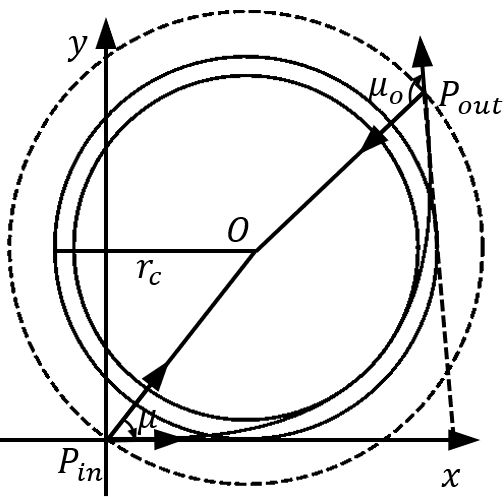
Figure 16: Characteristic angle and circle

The characteristic angle determines the characteristic circle, and the circle is furthermore helpful in determining the transit line between the first and third segments of the circular arcs. Like Dubins path, the second segment can be determined by the common tangent between the characteristic circles at the initial and final positions.

V Experimental Results

In this section, the computation method of Dubins path for the short distance case is tested and compared with the conventional method in terms of computation time. Then experiments are carried out for smoothing the trajectory. The minimum steering radius $r$ and the maximum sharpness $\sigma$ allowed by AMR are equal to $1$ and $0.6$, respectively, in the following text.

V-A Computation of Dubins path

Let the positions of the initial and final points, $P_{i}$ and $P_{f}$, be $(2.5,1)$ and $(4.5,1)$, respectively. Let the initial and final angle, $\theta_{i}$ and $\theta_{f}$, be $\pi/3$ and $\pi/4$, respectively. According to Section III, it is class $a_{11}$. Since $\alpha>\beta$, $q_{lsl}=0.67<\pi$, $S_{11}^{3}=2.88>0$ hold, according to Theorem 2, the type of the optimal trajectory is LSL. Actually, the length of all the existing trajectories are: $\mathcal{L}_{lsl}=7.86$, $\mathcal{L}_{rsr}=8.07$, $\mathcal{L}_{lsr}=13.56$, $\mathcal{L}_{rlr}=11.27$, $\mathcal{L}_{lrl}=11.78$, respectively. Therefore, LSL is indeed the shortest. The computation time is 0.043ms, while that of the conventional method is 0.137ms. The computation speed of this method is about 3 times faster than the conventional one. The trajectory is shown in Fig. 17.

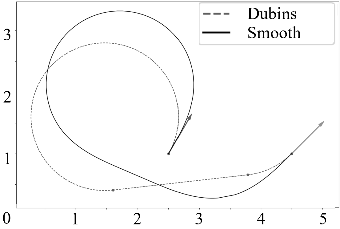
Figure 17: Trajectory of type of LSL in short distance case

V-B Smooth of Dubins path

Let the positions of the initial and final points, $P_{i}$ and $P_{f}$, be $(1,4)$ and $(9,4)$, respectively. Let the initial and final angle, $\theta_{i}$ and $\theta_{f}$, be $\pi/2$ and $\pi/3$, respectively. The type of the optimal trajectory is LSR. The trajectories are as shown in Fig. 18. Point $a$ and $b$ in the figure are the intersection points of line segment and circular arcs in the Dubins path. In the smooth trajectory, segments $P_{i}e$ and $fP_{f}$ are turns with continuous curvature. The curvature varies from $0$ to $\kappa_{max}$ and then back to $0$ again, as shown by the corresponding points in Fig. 19. It is easy to see that the two turns are both sharp(because the curvature reach the maximum $\kappa_{max}$). After smoothing, the problem that the curvature changes abruptly is well solved.

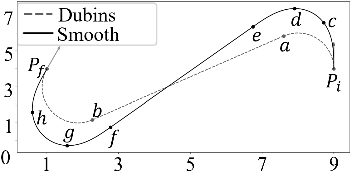
Figure 18: Trajectory of type of LSR in long distance case

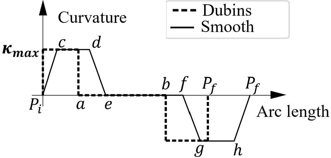
Figure 19: Curvature-arc length relationship corresponding to Fig. 18

Then consider the case of wide turn. Similarly, let $P_{i}=(1,1)$, $P_{f}=(9,1)$, $\theta_{i}=\pi/3$, $\theta_{f}=-2\pi/3$, respectively. The type of the optimal trajectory is LSL. Comparatively, the turn $fgP_{f}$ is a wide turn, because the maximum curvature of this turn is lower than $\kappa_{max}$.

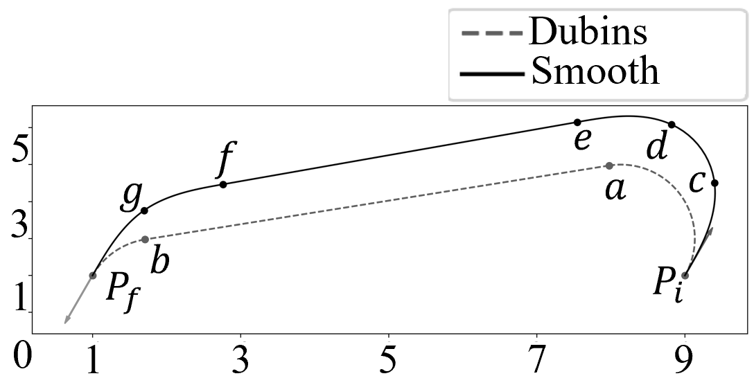
Figure 20: Trajectory of type of LSL in long distance case

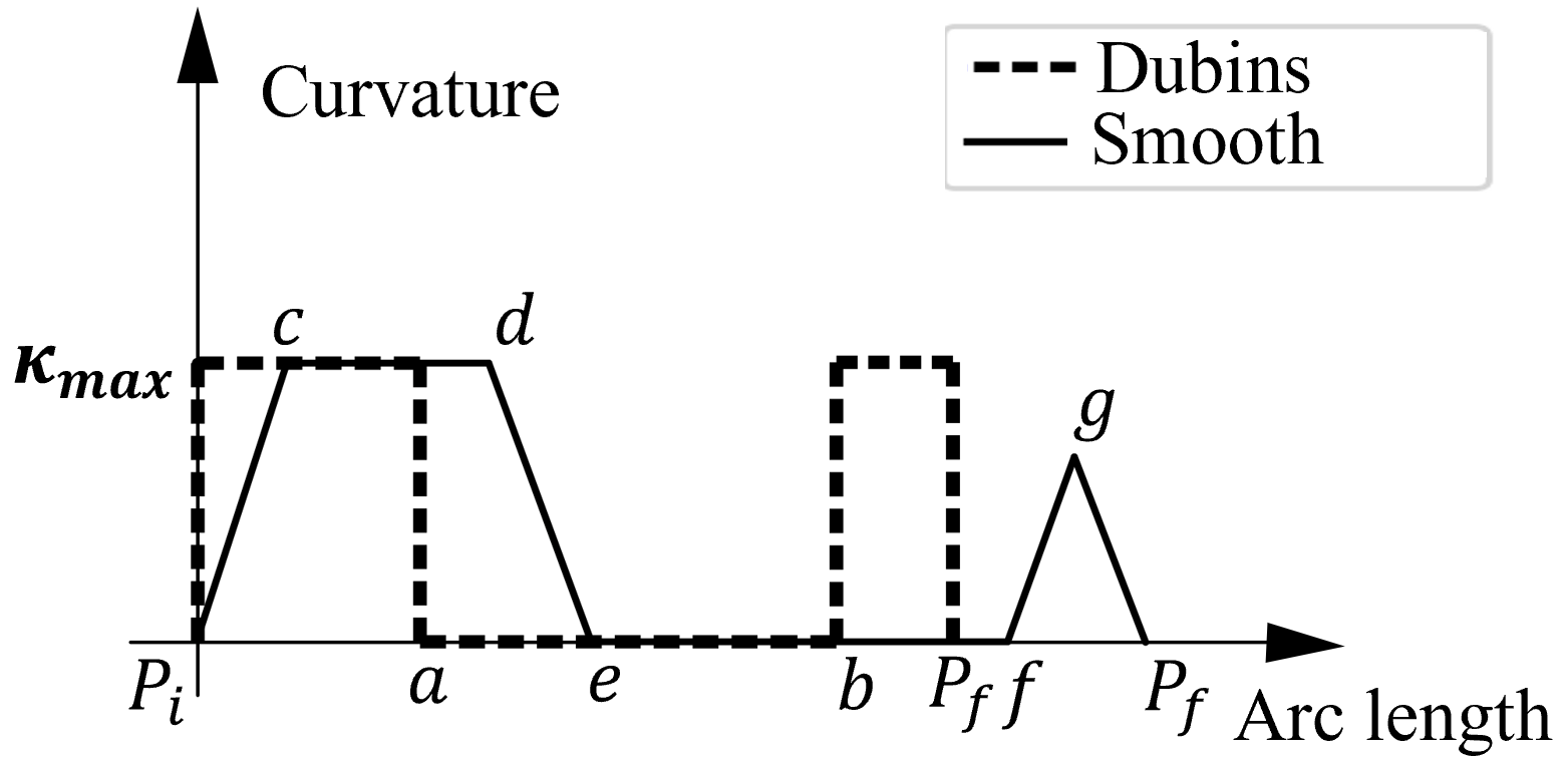
Figure 21: Curvature-arc length relationship corresponding to Fig. 20

VI Conclusion

In this paper, for the current problems of trajectory planning for logistics robots, we derived the fast calculation method of Dubins path for short distance and completed the calculation of Dubins path. To solve the problem of discontinuous curvature, we smoothed Dubins path by clothoid.

To calculate Dubins path in the case of short distance, the $16$ different combinations of angle quadrants are divided by topology into $6$ equivalency groups. Classes in the same groups have the same topology. The trajectory of a class can be easily obtained by orthogonally transforming the trajectory of any other class in the same group. This method is about three times faster than the conventional method, which greatly improves the efficiency.

We smooth the Dubins path for the discontinuous curvature problem. The turns are divided into sharp turn and wide turn by the angle and maximum curvature of the turn. By modifying the sharpness, the entry and exit points are on the same circle. In order to connect the two continuous turn, we presented the characteristic angle and furthermore the characteristic circle. Similar to Dubins path, the transit line can be determined by the common tangent of the two characteristic circles. The experiments show that the curvature varies linearly after smoothing.

References

- [1] Gasparetto A, Boscariol P, Lanzutti A, et al. Path planning and trajectory planning algorithms: A general overview[J]. Motion and Operation Planning of Robotic Systems: Background and Practical Approaches, 2015: 3-27.
- [2] van Gils T, Ramaekers K, Caris A, et al. Designing efficient order picking systems by combining planning problems: State-of-the-art classification and review[J]. European Journal of Operational Research, 2018, 267(1): 1-15.
- [3] Urmson C, Anhalt J, Bagnell D, et al. Autonomous driving in urban environments: Boss and the urban challenge[J]. Journal of field Robotics, 2008, 25(8): 425-466.
- [4] C. Zheyi and X. Bing, “AGV Path Planning Based on Improved Artificial Potential Field Method,” 2021 IEEE International Conference on Power Electronics, Computer Applications (ICPECA), Shenyang, China, 2021, pp. 32-37, doi: 10.1109/ICPECA51329.2021.9362519.
- [5] Xu X, Wang M, Mao Y. Path planning of mobile robot based on improved artificial potential field method[J]. Journal of Computer Applications, 2020, 40(12): 3508.
- [6] Liu X-H, Zhang D, Zhang J, et al. A path planning method based on the particle swarm optimization trained fuzzy neural network algorithm[J]. Cluster Computing, 2021: 1-15.
- [7] Sarkar R, Barman D, Chowdhury N. Domain knowledge based genetic algorithms for mobile robot path planning having single and multiple targets[J]. Journal of King Saud University-Computer and Information Sciences, 2022, 34(7): 4269-4283.
- [8] Kumar S, Sikander A. Optimum mobile robot path planning using improved artificial bee colony algorithm and evolutionary programming[J]. Arabian Journal for Science and Engineering, 2022, 47(3): 3519-3539.
- [9] Zheng L, Zeng P, Yang W, et al. Bézier curve-based trajectory planning for autonomous vehicles with collision avoidance[J]. IET Intelligent Transport Systems, 2020, 14(13): 1882-1891.
- [10] Shiller Z, Gwo Y-R, others. Dynamic motion planning of autonomous vehicles[J]. IEEE Transactions on Robotics and Automation, 1991, 7(2): 241-249.
- [11] Reeds J, Shepp L. Optimal paths for a car that goes both forwards and backwards[J]. Pacific journal of mathematics, 1990, 145(2): 367-393.
- [12] Barraquand J, Latombe J-C. Nonholonomic multibody mobile robots: Controllability and motion planning in the presence of obstacles[J]. Algorithmica, 1993, 10(2-4): 121.
- [13] Shkel A M, Lumelsky V J. Classification of the Dubins set[J]. Robotics Auton. Syst., 2001, 34: 179-202.
- [14] Dubins L E. On curves of minimal length with a constraint on average curvature, and with prescribed initial and terminal positions and tangents[J]. American Journal of mathematics, 1957, 79(3): 497-516.
- [15] H. Ren and K. Fujisawa, “Obstacle Avoidable G2-continuous Trajectory Generated with Clothoid Spline Solution,” 2021 6th International Conference on Control and Robotics Engineering (ICCRE), Beijing, China, 2021, pp. 23-27, doi: 10.1109/ICCRE51898.2021.9435729.
- [16] M. Brezak and I. Petrović, “Real-time Approximation of Clothoids With Bounded Error for Path Planning Applications,” in IEEE Transactions on Robotics, vol. 30, no. 2, pp. 507-515, April 2014, doi: 10.1109/TRO.2013.2283928.
- [17] G. Ignéczi and E. Horváth, “A Clothoid-based Local Trajectory Planner with Extended Kalman Filter,” 2022 IEEE 20th Jubilee World Symposium on Applied Machine Intelligence and Informatics (SAMI), Poprad, Slovakia, 2022, pp. 000467-000472, doi: 10.1109/SAMI54271.2022.9780857.
- [18] D. González, J. Pérez, V. Milanés and F. Nashashibi, “A Review of Motion Planning Techniques for Automated Vehicles,” in IEEE Transactions on Intelligent Transportation Systems, vol. 17, no. 4, pp. 1135-1145, April 2016, doi: 10.1109/TITS.2015.2498841.
- [19] D. K. Wilde, “Computing clothoid segments for trajectory generation,” 2009 IEEE/RSJ International Conference on Intelligent Robots and Systems, St. Louis, MO, USA, 2009, pp. 2440-2445, doi: 10.1109/IROS.2009.5354700.
- [20] T. Fraichard and A. Scheuer, “From Reeds and Shepp’s to continuous-curvature paths,” in IEEE Transactions on Robotics, vol. 20, no. 6, pp. 1025-1035, Dec. 2004, doi: 10.1109/TRO.2004.833789.