[1]\fnmPierre \surGaillard \equalcontThese authors contributed equally to this work.
These authors contributed equally to this work.
These authors contributed equally to this work.
1]\orgdivUniv. Grenoble Alpes, \orgnameINRIA, \orgnameCNRS, \orgnameGrenoble INP, \orgnameLJK, \orgaddress \cityGrenoble, \postcode38000, \countryFrance
2]\orgdivDEEL, \orgnameIRT Saint Exupéry, \orgaddress\street3 rue Tarfaya, \cityToulouse, \postcode31400, \countryFrance
3]\orgdivUMR5219, \orgnameInstitut Mathématiques de Toulouse, \orgaddress\street118 route de Narbonne, \cityToulouse, \postcode31400, \countryFrance
4] \orgnameTSE, \orgaddress\street1, Esplanade de l’Université, \cityToulouse, \postcode31000, \countryFrance
Adaptive approximation of monotone functions
Abstract
We study the classical problem of approximating a non-decreasing function in norm by sequentially querying its values, for known compact real intervals , and a known probability measure on . For any function we characterize the minimum number of evaluations of that algorithms need to guarantee an approximation with an error below after stopping. Unlike worst-case results that hold uniformly over all , our complexity measure is dependent on each specific function . To address this problem, we introduce , a generalization of an algorithm originally proposed by Novak (1992) for numerical integration. We prove that achieves an optimal sample complexity for any function , up to logarithmic factors. Additionally, we uncover results regarding piecewise-smooth functions. Perhaps as expected, the error of decreases much faster for piecewise- functions than predicted by the algorithm (without any knowledge on the smoothness of ). A simple modification even achieves optimal minimax approximation rates for such functions, which we compute explicitly. In particular, our findings highlight multiple performance gaps between adaptive and non-adaptive algorithms, smooth and piecewise-smooth functions, as well as monotone or non-monotone functions. Finally, we provide numerical experiments to support our theoretical results.
keywords:
-approximation, sequential algorithms, numerical integration1 Introduction
Let be any non-empty compact intervals in . The problem we consider in this paper is the following. Given any non-decreasing function that is initially unknown but that a learner can sequentially evaluate at points of their choice, how to best estimate with as few evaluations of as possible? We will study the error as a performance criterion, for some known integer and some known probability measure on . More precisely, we will study algorithms that can guarantee an error observably below after a finite number of evaluations, and will characterize the minimum number of such evaluations to reach this goal, for any non-decreasing function . Even though this problem is a classical one, finding the best -dependent sample complexity and an algorithm that achieves it is still an open question.
To make things more formal, we first describe how the learner interacts with the unknown function .
Online protocol.
Given an accuracy level , the learner first chooses a point , then observes , then chooses , then observes , etc. At each round , the point is chosen as a measurable function of the whole history . The process ends after a finite number of rounds whose value may be determined during the observation process ( is a stopping time).111This means that, for any integer , whether the inequality is true or not is fully known after observing (in a measurable way). Finally, after observing the whole history , the learner outputs a function as a candidate for estimating . We will call algorithm222Throughout the paper our definition of algorithms refers in fact to adaptive algorithms that adjust their sequence of points to the function to be approximated based on previous observations. The latter should be contrasted with non-adaptive algorithms, for which the sequence of points is fixed for all functions ’s. any procedure that, given and , returns a tuple in satisfying the above online protocol. We only consider deterministic algorithms, except for the integral estimation problem (Section 4.1) for which randomized algorithms achieve better rates in expectation.
Learning goal: small number of evaluations with guaranteed error.
Let be any positive integer and be any probability measure on . The performance of the learner will be evaluated by its error defined by
| (1) |
In all the sequel, an accuracy level will be initially given to the learner, who will be required to guarantee that after stopping, for any (initially unknown) non-decreasing function . Given this constraint, the goal of the learner is to make as few evaluations of as possible, that is, to minimize the stopping time . We will also refer to as the sample complexity of the algorithm.
Main intuitions and informal presentation of the results.
Before detailing our results in the next sections, we describe the main intuitions in the special case where and is the Lebesgue measure on . The ideas are introduced informally and will be made more precise later.
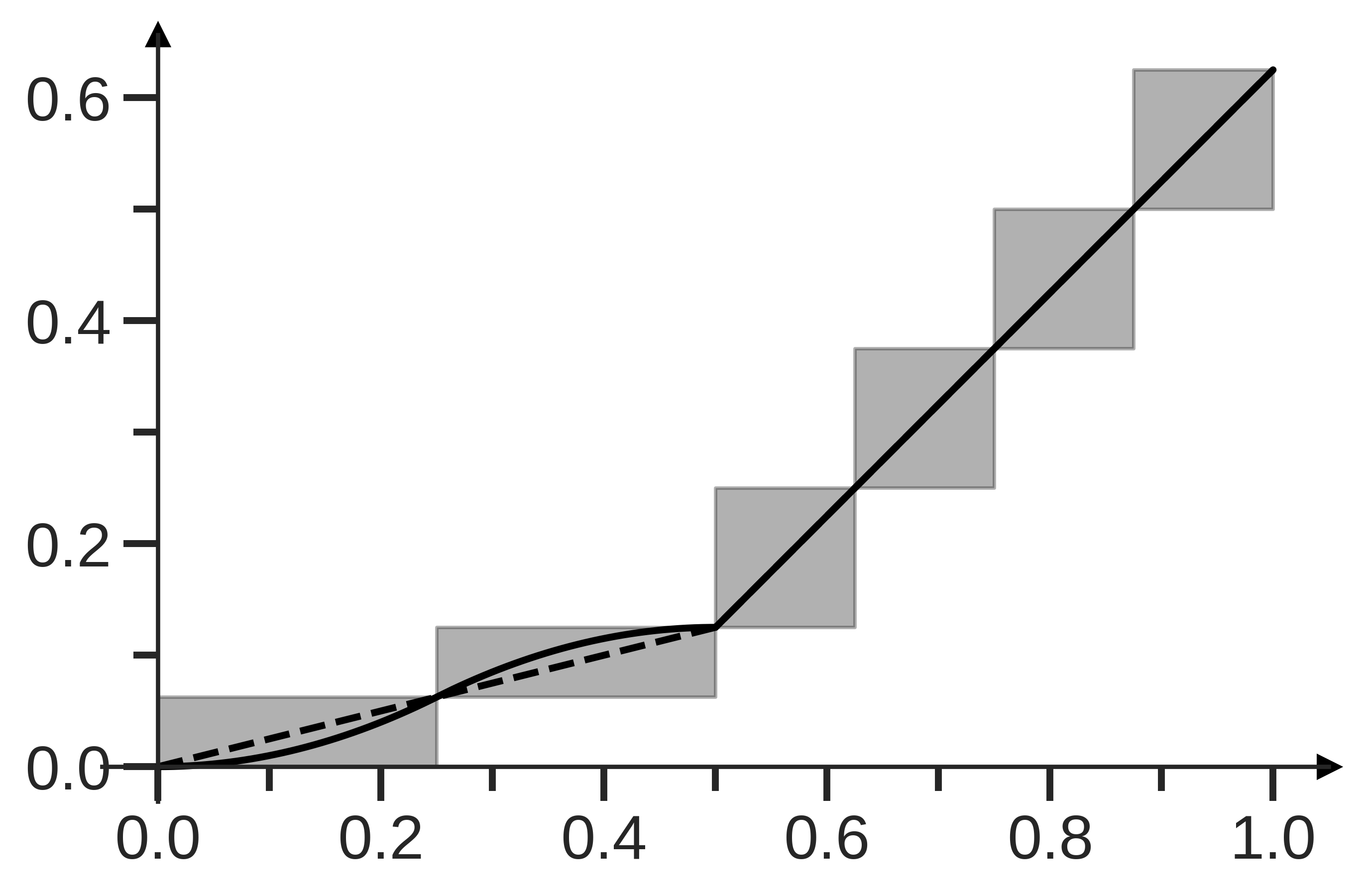
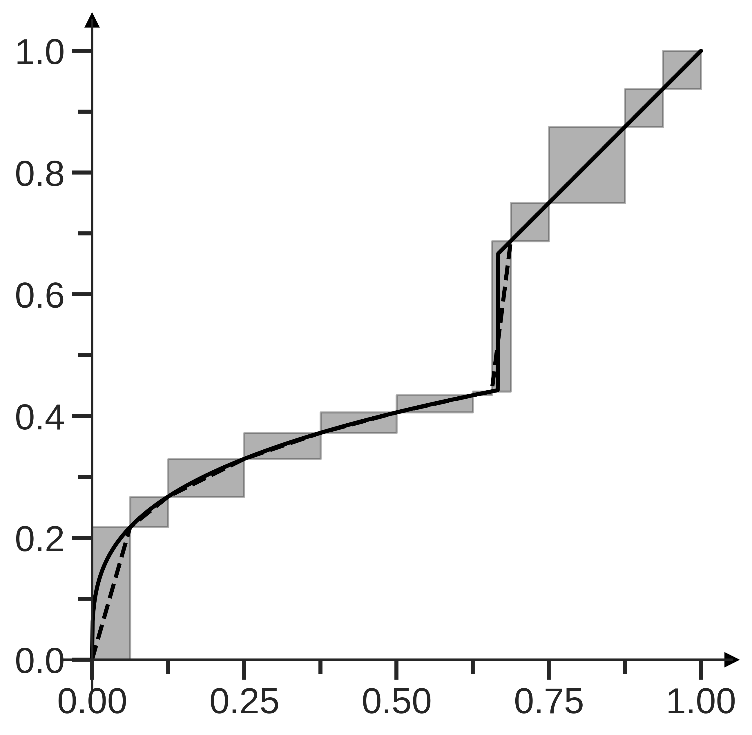
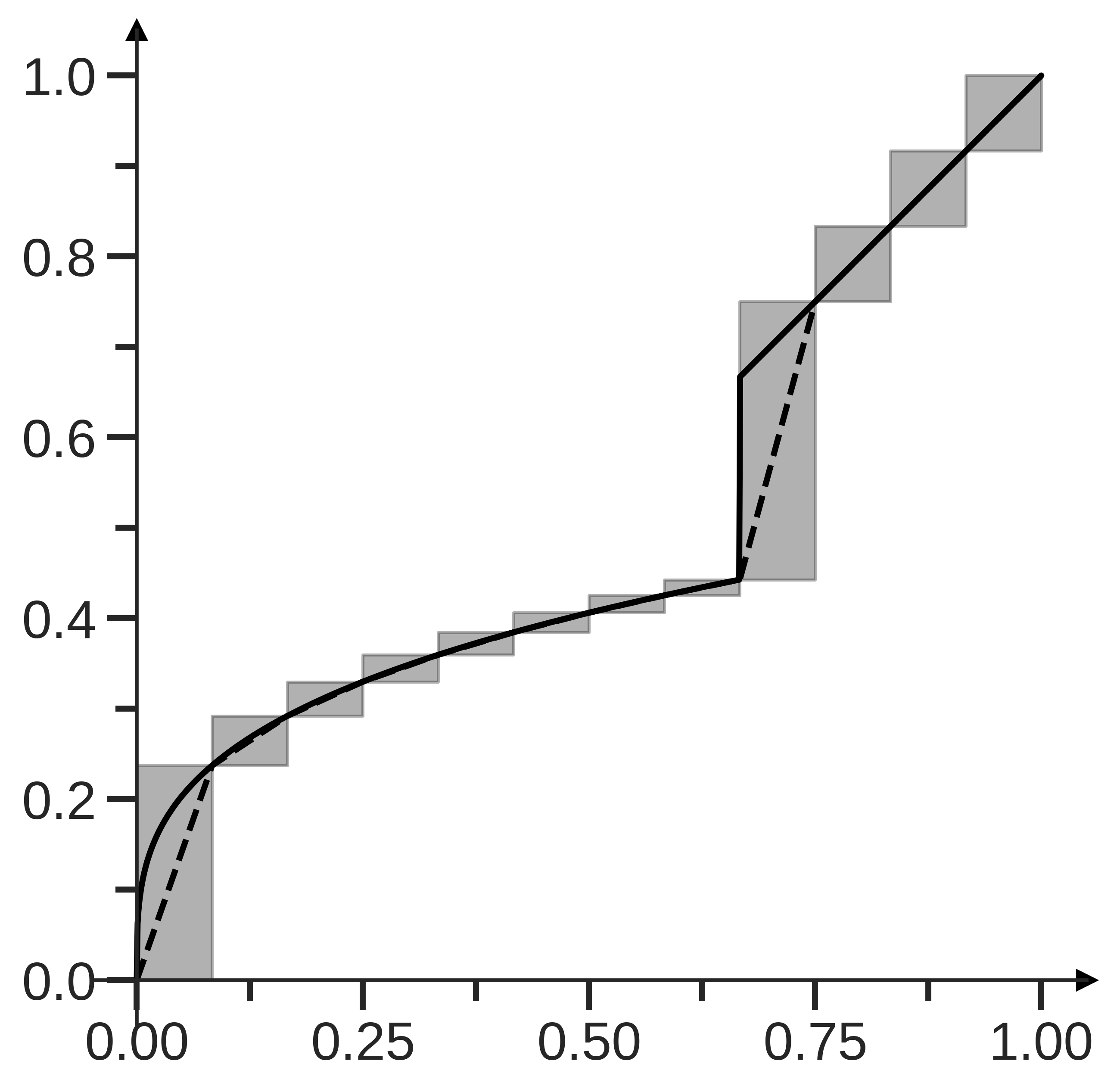
Imagine that we have already evaluated at some points . Since we know that is non-decreasing and bounded between and , we can deduce that the graph of is contained inside the adjacent rectangles (or boxes) shown in Figure 1.333Two boxes are degenerate (and thus not visible) on Figure 1, since GreedyBox evaluates at the endpoints and . Therefore, estimating with any function whose graph also lies in these adjacent boxes will guarantee an error of at most the total area of these boxes. We can even achieve by estimating with a piecewise-constant function (on each box , choose ) or with a piecewise-affine function (choose that linearly interpolates all the observed points ).
Now let , and suppose that we want to guarantee an error below as quickly as possible. Given the above comment, it seems that an ideal choice of the sequence is such that the total area of the adjacent boxes at round falls below for the smallest value of possible. We derive lower and upper bounds that support this intuition:
-
•
Lower bound: if after stopping (at time ) we want to guarantee that whatever , then must be larger than or equal to the minimum number (denoted by ) of adjacent boxes that contain the graph of and whose total area is at most of (see Theorem 1).
-
•
A nearly optimal greedy algorithm: of course an optimal choice of is impractical (it would require the full knowledge of the function ). However, a natural algorithm is to choose at each round the next point in the middle of the box with maximum area, so as to greedily reduce the total area of the boxes. See Figure 1 for an illustration. This algorithm, which we call , was suggested in a similar form by Novak [1]. One of our main contributions is to show that the stopping time of is always at most of the order of the lower bound up to a logarithmic factor in (see Theorem 2).
Both the lower and upper bounds are proved in a more general setting, in norm, for any integer and any probability measure on .
1.1 Contributions and outline of the paper
Our main contribution is to characterize the optimal sample complexity of algorithms with guaranteed error after stopping (see after Equation (1)), for any non-decreasing function , any and any probability measure . More precisely:
- •
-
•
In Section 3 we study GreedyBox (Algorithm 1) and show that its sample complexity matches our lower bound up to logarithmic factors (see Theorem 2). An important practical feature of GreedyBox is that, at each iteration , it provides a certificate that upper bounds its error and stops as soon as this certificate falls below .
All the results are written in the case where for convenience, but all of them can be rescaled to any non-empty compact intervals and of .444The case where is not closed can be addressed similarly via a simple extension argument and by replacing the values of at the endpoints of by the endpoints of .
In Section 4 we study consequences (with improved rates) for two specific subproblems:
-
•
Integral approximation. For this problem, we show that the deterministic version of GreedyBox (Algorithm 1) is also optimal up to logarithmic factors. However, drawing inspiration from Novak [1], we introduce a randomized version in Section 4.1.2 that improves the accuracy by a factor of in expectation after iterations (Theorem 4).
-
•
Worst-case function approximation under a smoothness assumption. In the worst case, the upper bound of Theorem 2 is of the order of for monotone functions. It is well known that for smooth functions, better rates can be achieved using improved quadrature formulas (e.g., Davis and Rabinowitz [2]). For example, functions can be -approximated in any norm after roughly evaluations (also discussed in Appendix B.8). In Section 4.2, we provide a minimax lower bound showing that function evaluations are necessary for any algorithm seeking to approximate a piecewise-affine function with singularities (see Proposition 6). We establish that GreedyBox in fact achieves this rate for piecewise- functions when , but is suboptimal in the regime (Theorem 5 and Proposition 7). Lastly, we propose a simple modification of GreedyBox that optimally addresses both regimes. These results highlight three significant differences for the -approximation problem:
-
–
between monotone piecewise- functions with two or more discontinuities, for which a better rate than is not achievable, and functions (with no singularities) which can be approximated at a rate of ;
-
–
between general piecewise- functions and monotone piecewise- functions, with a minimax rate respectively of at least and at most for ;
-
–
between non-adaptive algorithms, which need function evaluations, and adaptive ones, which only require for .
-
–
Finally, in Section 5, we provide numerical experiments that compare GreedyBox to the trapezoidal method on several functions . Our simulations validate the rates anticipated by our analysis and demonstrate the superiority of our approach compared to the uniform trapezoidal rule in approximating monotone piecewise-smooth functions within the norm.
1.2 Important definitions and notation
We now introduce several definitions and notations that will be useful to present our results more formally. In all the sequel, we work with , some fixed integer and a probability measure on .
Standard notation.
We denote by the set of integers greater than or equal to . For any , we denote the floor and ceiling functions at by and respectively. For any measurable function , we denote the -norm of by .
Box, width, generalized area.
We call box any subset with and . Its width is given by
and its generalized area is given by
Note that the above definitions consider open intervals . The generalized area corresponds to the usual notion of area when and is the Lebesgue measure.
Adjacent boxes.
We denote by the set of all boxes. We say that a finite sequence of boxes are adjacent if and only if they are of the form for all , for some sequence .
Box-cover and box-covering number of a function.
Let be any non-decreasing function. We call box-cover of any sequence of adjacent boxes that contains the graph of except maybe at the boxes’ endpoints, i.e., writing as above, such that . Furthermore, given , we define two complexity quantities:
-
(i)
denotes the minimum cardinality of a box-cover of whose generalized areas satisfy . We call this quantity the box-covering number of at scale .
-
(ii)
denotes the minimum cardinality of a box-cover of with generalized areas for all .
All our main results will be expressed in terms of ; the other quantity will however be useful in the proofs. The connections between the two are described in Appendix A.3.
We now reinterpret the condition appearing in (i) in an equivalent way. When , this condition corresponds to the total area of the boxes being bounded by (as mentioned earlier in the introduction). For general , an equivalent and useful formulation is the following. Denote by , , the boxes of the cover, and by and the best known lower and upper bounds on the function inside the boxes . Then, is equivalent to
| (2) |
The last condition implies that and are good lower and upper bounds on the function outside of the points . Note an interesting connection with the definition of bracketing entropy in empirical processes theory (see, e.g., [3, Chapter 19] and references therein).
The following lemma shows that is always well defined and at most of the order of . The proof is postponed to Appendix A, where we collect other useful properties about .
Lemma 1.
For all non-decreasing functions and , the quantity is well defined and upper bounded by
| (3) |
Though the rate of is tight in the limit for many functions such as and probability measures such as , the asymptotic behavior of when does not necessarily reflect the shape of for a given . Indeed all functions which are -close to some piecewise-constant function have a very small box-covering number , even if is large in the limit . Importantly, as we show in the next sections, the estimation problem addressed in this paper is very easy for such functions and scales .
1.3 Related works
Quadrature formulas (approximation formulas for the computation of an integral) have long been studied for diverse classes of functions and algorithms along the past decades. We focus on references with strong connections to our problem. Sukharev [4] proved that affine methods are minimax optimal in the set of nonadaptive methods for every convex set of functions. It is in particular the case for non-decreasing functions. Since the work of Bakhvalov [5], it is known that nonadaptive methods are as good as adaptive ones for any class of functions that is both convex and symmetric. Note that the last hypothesis is not verified in our problem. However, Kiefer [6] later showed that the trapezoidal rule is optimal among all deterministic (possibly adaptive) methods for integral approximation in the case of monotone functions. His work was completed by the one of Novak [1], who gave optimal bounds for different possible types of algorithms as summarized in Table 1. In particular it is shown that adaption combined with randomization is key to obtaining an improved rate in expectation. These bounds were later extended by Papageorgiou [7] to the integral approximation of multivariate monotone functions. The books from Davis [2] and Brass [8] give a larger panel of results on numerical integration under various assumptions.
| Strategy | Non-adaptive | Adaptive |
|---|---|---|
| Deterministic | ||
| Stochastic |
Of course, many other function sets were studied. A non-exhaustive list includes work on the set of unimodal functions [9], on the set of functions with bounded variation [10], on convex and symmetric classes of functions [11, 12, 13], and on various classes of multivariate functions [14, 15, 16]. Note that the bounds in the previous papers are not -dependent.
All of the aforementioned works were on integral approximation, an easier problem than approximation. Numerous studies investigate the approximation of diverse classes of functions, mostly using interpolation. A known example is polynomial interpolation for -times continuously differentiable functions. Many works employ the modulus of smoothness of the function to bound its approximation, providing -dependent bounds. It is for example the case of [17] for the approximation of periodic functions using trigonometric polynomials. The computation of a best linear -approximation, where a basis of functions is previously given and one looks for the weights that minimize , was studied in depth (e.g. [18, 19]). [20] studied the class of functions with their first derivatives continuous except at one singularity, and showed that adaptive algorithms are better that non-adaptive in the case of integral estimation. The same remark and work was later carried to approximation in [21]. Some work involves -monotone functions, that is, functions with monotone -th derivatives. The papers [22, 23] studied the rate of convergence of interpolation methods on this set of functions, and showed results depending on the modulus of smoothness of the function. To our knowledge, little is known about approximation of general non-decreasing functions, without any continuity or smoothness assumptions.
Adaptive methods have a long history in numerical integration and other approximation or learning problems. For numerical integration of monotone functions, as mentioned above, adaption combined with randomization is key to improving worst-case rates (see [1] and Table 1 above, as well as [24]). We show that adaption is also key to obtaining less pessimistic, -dependent error bounds. This work also shares algorithmic principles with online learning methods for (possibly noisy) black-box optimization, such as bandit algorithms [25] or the EGO algorithm [26]. Indeed such algorithms rely on adaptive sampling strategies to reduce the current uncertainty (via, e.g. UCB or Bayesian approaches), which is reminiscent of the way GreedyBox selects the box to be split at time . Close to our paper is the work by Bachoc et al. [27], who derive -dependent error bounds for certified black-box Lipschitz optimization.
Lastly, Bonnet et al. [28] explore a close variant of our main algorithm (Algorithm 1), which itself draws significant inspiration from Novak [1] for numerical integration. Bonnet et al. [28] address the problem of adaptively reconstructing a monotone function from imperfect observations. In contrast to our approach, they do not provide any guarantees regarding sample complexity or approximation. Their focus is on asymptotic convergence guarantees, including point-wise, , or norm convergence, as the number of function evaluations tends towards infinity. They do not provide any convergence rate information, nor finite time or f-dependente guarantees. Nevertheless, they highlight an intriguing application in uncertainty quantification that could potentially benefit from our analysis.
2 Lower bound
In this section we prove a lower bound on the number of evaluations of that any deterministic algorithm must request in order to guarantee an -approximation of in -norm after stopping, when only given the prior knowledge that is non-decreasing. The next theorem states that in such a case, at least evaluations of are necessary.
In the sequel we write to make it explicit that the stopping time of the algorithm depends on the underlying function (through the sequentially observed values ).
Theorem 1.
Let and be the output of any deterministic algorithm such that, for all non-decreasing functions ,
Then, for all non-decreasing functions ,
In words, any algorithm that is guaranteed to output an -approximation after finitely-many evaluations whatever the non-decreasing function must evaluate each at least times before stopping. In Section 3 we show a matching upper bound up to a multiplicative factor of the order of . This indicates that the box-covering number introduced in Section 1.2 is a key quantity to describe the inherent difficulty of the estimation problem.
Note that the lower bound holds for every simultaneously. It thus has a similar flavor to distribution-dependent lower bounds that have been proved for the stochastic multi-armed bandit problem in online learning theory (see, e.g., Chapter 16 by Lattimore and Szepesvári [25]). Recently an -dependent lower bound (also based on a notion of cover) was proved by Bachoc et al. [27] for certified zeroth-order Lipschitz optimization, where algorithms are required to output error certificates (i.e., observable upper bounds on the optimization error).
Proof.
Assume for a moment that there exists a non-decreasing function such that . When run on , the algorithm only uses the query points before stopping. Let denote the ordered values after removing redundancies and the values and (if applicable), with . Consider the adjacent boxes for where we set and . The sequence is a box-cover of (by monotonicity). We construct two functions and that surround :
Since for all , the algorithm (which is deterministic) would behave the same when run with or as when run with , and would construct the same approximation function after the same number of evaluations. However,
where the last inequality follows from and the definition of . The triangle inequality then yields
which shows that one of or is larger than . Since (as proved above) is the approximation function output by the algorithm both with and , which are both non-decreasing, the last conclusion is in contradiction with the assumption that for all non-decreasing functions . This concludes the proof. ∎
3 Upper bound
In this section we introduce the GreedyBox algorithm and derive an -dependent sample complexity bound (Theorem 2) that matches the lower bound of Theorem 1 up to a logarithmic factor, for every non-decreasing function . In Section 4 we will study consequences and derive improved bounds for integral estimation (in expectation) and worst-case approximation of piecewise- functions.
3.1 Algorithm and main result
We consider Algorithm 1 below, which draws heavily on an algorithm proposed by Novak [1, Section 3.2] for numerical integration, and which we call thereafter. A variant for handling imperfect observations was also considered by Bonnet et al. [28].
It is remarkably simple: at every round, it selects the largest box in the current box-cover of and replaces it with two smaller boxes by evaluating at the middle or, more generally, at a conditional median for a general probability measure . At any , we approximate with the trapezoidal estimator defined as the piecewise-affine function that joins the points visited up to time . Note that this estimator uses evaluations of . We stop Algorithm 1 at time , which is the first when the certificate falls below . (This is because is a valid upper bound on , by Lemma 2 below.)
-
1.
Select a box with largest generalized area: pick .
-
2.
Let be a median of the conditional distribution , and evaluate at .
-
3.
Sort the points in increasing order:
. -
4.
Define the generalized areas for all by
-
5.
Update the certificate
(4) -
6.
Let .
Output: .
Algorithmic complexity.
We assume that a median of the conditional distribution can be computed exactly at every round . When is the Lebesgue measure, it can indeed be computed in closed form: it is the midpoint .
For the sake of simplicity, in Algorithm 1 we perform a sort (Step 3) and an argmax operation (Step 1) at each round , to get the points in increasing order and to choose the box with the largest generalized area. However, one can get rid of the sort operation at each round and do it only once at the end, because GreedyBox does not need the order of the boxes before the last iteration, where it uses sorted points to build . Furthermore, for the argmax operation, naive methods yield a computational complexity of at each time , resulting in a quadratic complexity for , far worse than the linear complexity of traditional algorithms such as the trapezoidal rule. To speed up , we use a classical algorithmic trick: a max-heap, which is a binary tree that takes logarithmic time to both remove the maximum value and add an element. This provides with a computational complexity of after rounds, which is closer to the complexity of the trapezoidal rule.
Upper bound on the sample complexity.
Let be some target accuracy level. The next theorem provides a bound on the sample complexity of . The proof appears in Section 3.2.
Theorem 2.
Let be non-decreasing,555Recall that the input and output sets of can be rescaled to any non-empty compact intervals and of , changing the results only by a multiplicative constant. , and . Then, defined above (Algorithm 1) satisfies
at the stopping time . Furthermore, its sample complexity is bounded as follows:
We make three comments before proving the theorem.
A new -dependent bound. Since for all non-decreasing functions (by Lemma 1), the above sample complexity bound implies the well-known upper bound of up to logarithmic factors in the worst case. Importantly, though the rate of is worst-case optimal (see, e.g., [6, Section 5.A]), Theorem 2 yields a much better bound for functions that are easier to approximate, such as functions close to piecewise-constant functions, because is small in that case. Since the algorithm uses no prior knowledge on (beyond monotonicity) to stop at , it is adaptive to the unknown complexity .
A nearly optimal bound. Note that the lower bound of Theorem 1 is in terms of , while the upper bound of Theorem 2 is proportional to . By a simple argument (dividing boxes times to reduce their generalized widths by a factor of , similarly to the proof of Lemma 4), we can prove that . Therefore, the lower and upper bounds of Theorems 1 and 2 match up to a logarithmic factor. For each non-decreasing function , GreedyBox is thus nearly optimal among all algorithms with guaranteed error after stopping.
A possible minor improvement. When is the Lebesgue measure, the bound on could be slightly improved (in the constants) by replacing the certificate in Equation (4) with (see Lemma 9 in Appendix B.1). While a similar minor improvement is likely to hold for general with a slightly different interpolation (non-necessarily piecewise-affine), we decided to focus on piecewise-affine interpolations for the sake of presentation.
3.2 Proof of Theorem 2
Before proving Theorem 2, we first state three lemmas, whose proofs are all postponed to Appendix B.
The first one below shows that, at any round before stopping, the error of is at most the sum of the generalized areas to the power of the current-box cover of . We recall that denotes the generalized area of the -th box at round , and we define the trapezoidal estimato to be the piecewise-affine function that joins the points visited up to time .
Lemma 2.
Let be non-decreasing, and . For any ,
The next two lemmas are used to control . We first show (by a dichotomy argument) that the algorithm can quickly make all boxes equally small. Recall from Section 1.2 that denotes the minimum cardinality of a box-cover of for which each box has a generalized area below .
Lemma 3.
Let be non-decreasing, and . Define , and assume that is such that . Then, at time , all the boxes maintained by have a generalized area bounded from above by , i.e., for all .
The next lemma shows that the certificate at round decreases at least linearly in .
Lemma 4.
Let be non-decreasing, and . For any , we have . Therefore, for all in ,
| (5) |
Proof of Theorem 2.
We are now ready to prove the theorem. The first inequality follows immediately from Lemma 2 and from the fact that by definition of .
We now show by contradiction that . Assume thus for a moment that
| (6) |
This assumption will be used implicitly when calling Lemmas 3 and 4 below, since it will imply that (so that the algorithm has not stopped before any round considered below). We will see in the end that it raises a contradiction.
Let . By Lemma 3 applied with , at time , the boxes maintained by all have generalized areas at most of each, so that the certificate satisfies
| (7) |
where we used the fact that (by Lemma 8 in Appendix A.3) and that (since ). Now, we apply Lemma 4 with and . It yields:
This raises a contradiction with (6), since (using again )
and is by definition the first time such that . Therefore, (6) must be false, so that . Elementary calculations conclude the proof of Theorem 2. ∎
4 Improvement for special cases
In this section, we derive consequences (with rates faster than the worst-case ) in two specific cases: integral estimation and piecewise-smooth functions.
In the sequel, we adopt a slightly different yet equivalent viewpoint than in Section 3. Though Algorithms 2 and 3, defined in this section, formally stop at round , in the proofs, we extend their definitions to all rounds , by replacing the while condition with , defining as the first round (if any) where the certificate reaches , and setting for all subsequent rounds . Note that their approximation error equals zero for all .
4.1 Side problem: integral estimation
Throughout this subsection, we focus on the case of integral estimation rather than approximation in -norm. The goal is to approximate the integral of a non-decreasing function on . This problem is simpler than the -approximation problem studied previously, and thus can be easily extended to integral estimation while maintaining the same bound.
A deterministic algorithm for the integral estimation problem is defined as a procedure that, given , produces a tuple , where and are defined sequentially, similar to the approximation in -norm. That is: for all , is a measurable function of the history and is a stopping time after which the process of the algorithm ends. The algorithm finally outputs an approximation of the integral. We now study the convergence speed of in this setting (we replace the definition of in the last line of GreedyBox by the computation of ) and check whether it achieves optimal convergence speed.
4.1.1 Nearly optimal performance for integral estimation
The following upper bound on the sample complexity of GreedyBox is a direct consequence of Theorem 2 with .
Corollary 1.
Let be non-decreasing, and . Then, with satisfies, at the stopping time ,
Besides, its sample complexity is bounded from above as follows:
The question is now to check if the lower bound for this weaker problem is still the same one. The following theorem asserts that this is the case.
Theorem 3 (Matching lower bound).
Let and be any deterministic algorithm such that, for all non-decreasing functions :
Then, for all non-decreasing functions
4.1.2 Improvement in expectation with randomization
We now provide a stochastic version of our algorithm; see Algorithm 2 below, which we call . With this randomized variant we prove better guarantees (in expectation only)666We could easily derive high probability bound using Hoeffding’s lemma. for the integral estimation problem than with the deterministic version. Note that the improvement is not true for estimating in -norm. The idea to use randomization to improve the rates is due to Novak [1, Section 2.2]; we adapt this idea to a fully sequential algorithm, whose bound is now adaptive to the complexity of . It’s worth mentioning that, for the sake of simplicity, the random points in Algorithm 2 are currently sampled at the conclusion of the algorithm. However, an alternative approach could involve sequential sampling when the intervals are created, in order to get a sequential estimator for all .
-
1.
Select the box with the largest area: find .
-
2.
Let be a median of the conditional distribution and evaluate at .
-
3.
Sort the points in increasing order:
Define the boxes areas for by
Update the certificate
Let .
The following lemma shows that the error of (Algorithm 2) at stopping time is indeed at most .
Lemma 5.
Let and let be non-decreasing. Then, the output of Algorithm 2 satisfies
Proof.
First, we remark that the stopping time and the ordered sequence are deterministic and do not depend on the randomness of the algorithm. These deterministic points being set, the random variables for are distributed according to conditionally to each of the deterministic intervals defined by the ’s and satisfy for all
Therefore,
and
| (8) |
But since , by monotonicity of , takes values into the interval . Thus,
by definition of (see step 3 of Algorithm 2). Therefore, substituting into Inequality (8) and taking the square root, we get
which is smaller than by the stopping criterion. ∎
Remark that if all boxes at time have similar areas (which the algorithm aims at getting by splitting only largest boxes), Lemma 5 is asking to be at most of order in Algorithm 2, while Algorithm 1 required . Therefore, this leads to an earlier stopping criterion and smaller sample complexity. Typically, after rounds, the approximation error of Algorithm 2 is better than the one of Algorithm 1 by a factor . This is however not so simple to formulate in terms of sample complexity. We will thus only formulate the analog of Theorem 2 under the following assumption.
Assumption 1.
Let . There exist and such that for all .
It is worth to notice that Assumption 1 is mild since for any non-decreasing and . Furthermore, the assumption is non-asymptotic in since the requirement is only for .
Theorem 4.
4.2 An intriguing result for piecewise-regular functions
For the sake of simplicity, in this section, we restrict ourselves to the Lebesgue measure.
As seen before, has a worst-case sample-complexity of order up to logarithmic factors. An interesting question is how the error rate improves with regularity for non-decreasing functions, as well as how to adapt to achieve optimal rates for piecewise-smooth functions. More precisely, unlike the rest of the paper, in this section, we focus on analyzing the effective -error rate of algorithms when run on piecewise-smooth functions. We control the number of evaluations of until falls below , rather than the number of evaluations until the certificate falls below . The first (classical) complexity quantity can be much smaller than (since the algorithm is only aware that is non-decreasing, and lacks any prior regularity knowledge). This does not contradict the lower bound of Theorem 1 and reveals the effective performance of algorithms when run on simpler functions. For instance, on functions, the trapezoidal rule has an effective rate of order (a classical result recalled in Appendix B.8), but cannot guarantee -accuracy before order evaluations if only given the knowledge that the underlying function is non-decreasing.
Upper bound on GreedyBox effective sample complexity.
We aim to explore an intriguing question: can we establish these guarantees for GreedyBox without making any modifications? Moreover, the trapezoidal rule fails to adapt to piecewise- functions, even for simple ones such as . On the contrary, adapts very well to the discontinuities: it converges exponentially fast for any piecewise-constant function. With this in head, one could ask if learns the jumps quickly enough to ensure an -accurate error within sample-complexity for piecewise- functions.777The notation hides logarithmic factors. The next theorem shows that the rate can indeed be improved as long as the number of -singularities888We call -singularity of a point such that is not on any neighborhood of . A discontinuity is a -singularity. is at most of order . It should be noted that the number of -singularities may explode to infinity as approaches zero and that the number of -singularities does not affect the upper bound.
Theorem 5.
Let and . Let be a non-decreasing and piecewise- function with a number of -singularities bounded by and such that whenever it is defined. Then, there exists
such that for all , where is the approximation of returned by after rounds.
Theorem 5 shows that, for piecewise- functions with , achieves -accuracy in function evaluations which improves the worst-case guarantee of Theorem 2. In particular, when the number of singularities is finite, then when , and the -error is asymptotically of order . Note that this result contrasts with what happens for piecewise- functions without the non-decreasing assumption considered by [21], who showed that as soon as there are strictly more than one discontinuity, any algorithm has a worst-case -error of order .
Minimax lower bound for approximating non-decreasing piecewise-smooth functions.
Interestingly, we now show that this result is optimal (up to logarithmic factors) among deterministic algorithms in the regime (Proposition 6), that is when the number of -singularities is at least of order . In the other regime, which corresponds to more regular functions, we also show that our upper bound on GreedyBox cannot be improved (Proposition 7).
Proposition 6.
Let , and . Then, for any deterministic adaptive algorithm and for any
there exists a non-decreasing piecewise-affine function with at most discontinuities, such that .
Remarkably, the above lower bound demonstrates a clear difference between regular functions and piecewise-regular functions, even when the number of pieces is finite. Specifically, when considering the case of , the above lower bound shows that, for piecewise- function with a constant number of discontinuities (), surpassing the bound of is not achievable. This demonstrates the influence of singularities, as functions with no singularities can be approximated at a rate . It is also worth pointing out that the above lower bound maybe easily extended to non-adaptive algorithms (considering Heaviside step adversarial functions) which would require function evaluations. This underscores, in a new scenario, the need of adaptive algorithms to approximate functions with singularities [21].
Negative result for GreedyBox.
The previous result shows that GreedyBox is (up to logs) optimal for highly non-regular functions (). We now consider the other regime () and prove an almost (up to logs) matching lower bound in the case , . This, shows that the rate cannot be improved for GreedyBox for such classes of functions.
Proposition 7.
Let . Then, there exists a piecewise- function with whenever it is defined and one -singularity, such that there exists with , where is the approximation after rounds.
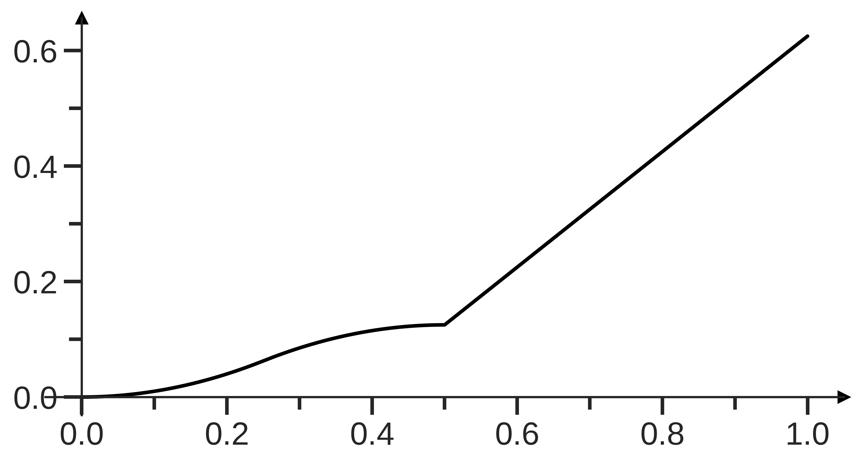
An example of the worst-case function built in the proof of Proposition 7 for , that exhibits poor performance for GreedyBox at , is depicted in Figure 2. The function is formally defined in the proof and consists of two parts: one that oscillates with for , and the other that is linear for . The function is constructed in such a way that at a certain ( in Fig. 2), GreedyBox selects its points precisely between the oscillations, and focuses too much on the linear part, resulting in a maximum possible error. It is worth noting that for each value of , it is possible to construct an adversarial function . However, an interesting question arises: can a single function be devised to work uniformly for all values of ? We believe that this question is challenging and connected to the 10th open problem raised in [8, Chapter 10].
GreedyWidthBox: an optimal modification of GreedyBox.
GreedyBox can actually be adapted to achieve the optimal rate of simultaneously for all , while maintaining our adaptive guarantee in terms of . This can be accomplished by employing the GreedyBox approach for half of the iterations and the trapezoidal rule for the remaining half (see Algorithm 3). The proof, left to the reader, follows closely the one of Theorem 5, in which the upper bound (17) can be simplified by utilizing the fact that, after conducting function evaluations, the trapezoidal rule ensures that all widths are at most of the order . In particular, for and , this provides an algorithm that achieves -acccuracy in norm in function evaluations for non-decreasing piecewise- functions, as soon as the number of -singularities remains constant as .
-
1.
if is even then
Evaluate at the midpoint . 3. Sort the points in increasing order:
Define the generalized areas for all by
Update the certificate
Let .
5 Numerical Experiments
In this section, we study empirically the performance of as compared to the trapezoidal rule. All the experiments are run using and the Lebesgue measure for . Figure 3 displays the output given by both and the trapezoidal rule on the function defined by if and otherwise. One can see that on this example the error of is twice as small as that of the trapezoidal rule. In general, copes far better with discontinuities than the trapezoidal rule.
Remark that the trapezoidal rule is usually an offline algorithm that needs the total number of iterations from the beginning. Fortunately, it can easily be adapted to an online version built on the same model as . Instead of choosing the box with the largest area on Step 1 of , it picks the box with the largest width. This online version matches exactly the offline trapezoidal rule whenever is a power of and allows for a better comparison with . It is this online version that we use in the next experiments.
The trapezoidal rule is known to have an error that decreases linearly with the number of iterations for any non-decreasing functions. This is the same speed of convergence that we proved for in Theorem 2. However, for functions, the error of the trapezoidal rule decreases quadratically with the number of iterations, which corresponds to a sample complexity . This is better than the upper bound in proven in Theorem 5 for . Remember however than no lower bound of order was proved so far for on functions with no singularities. Also note that the trapezoidal rule achieves a rate of only for functions, but can have an error of order as soon as the function is discontinuous (see Figure 4(c)).
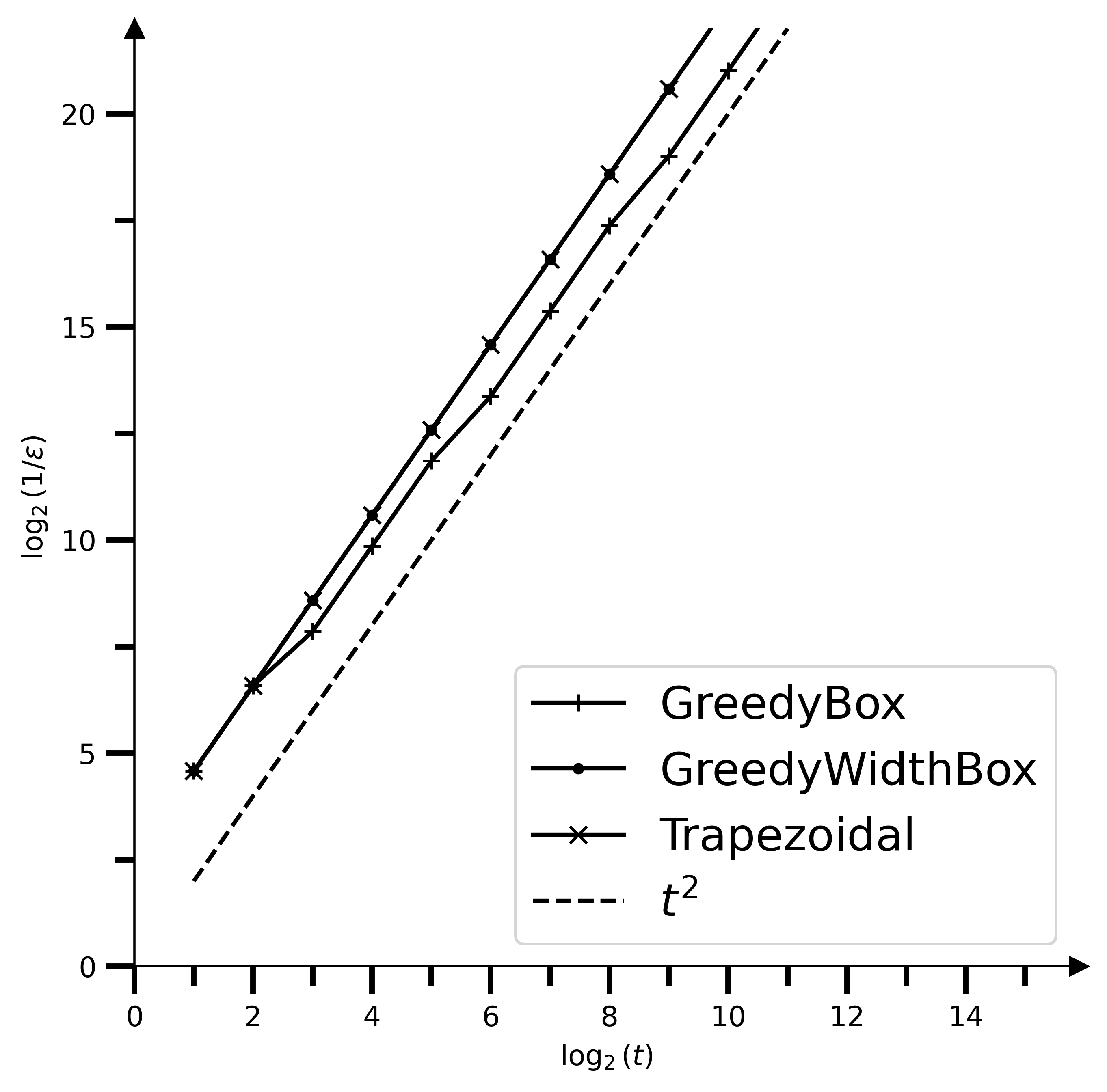
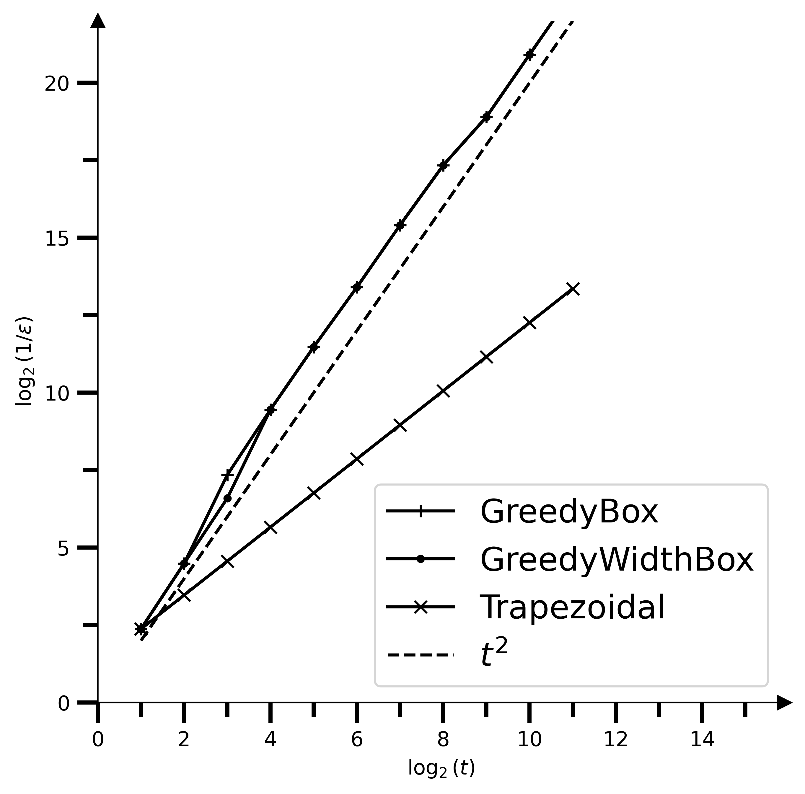
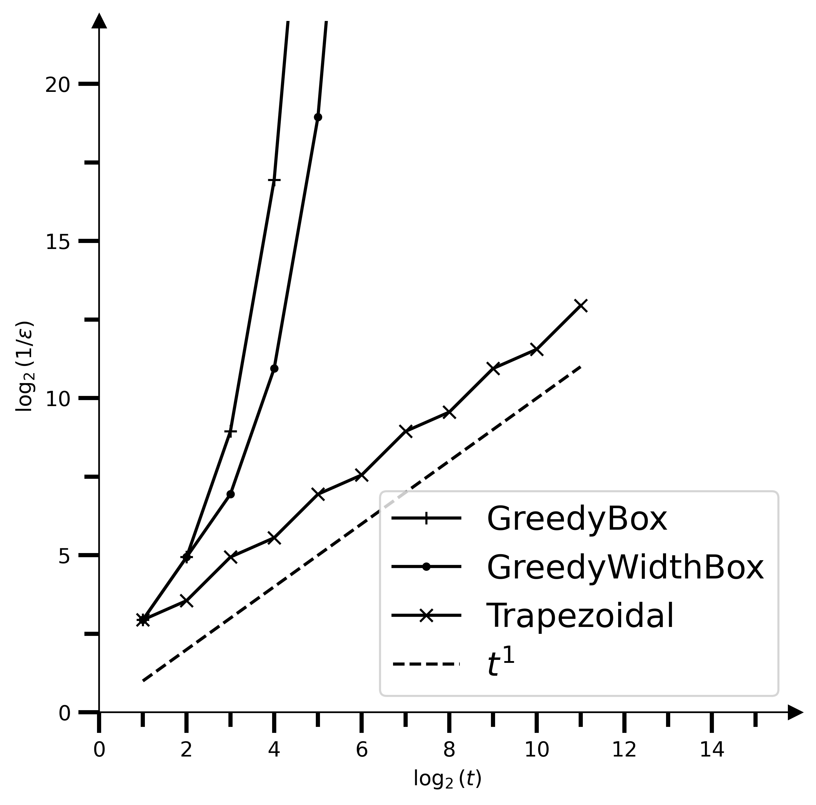
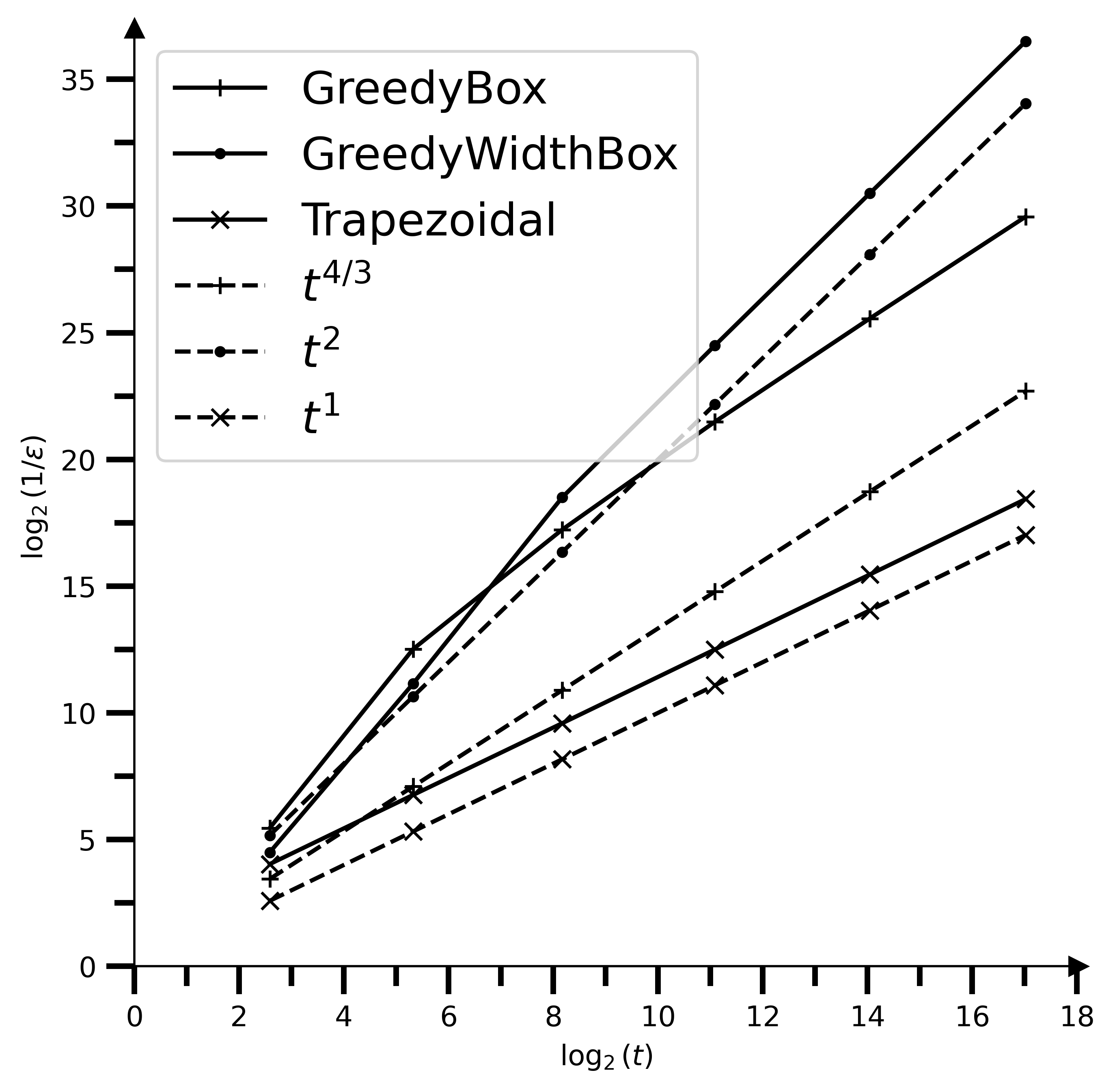
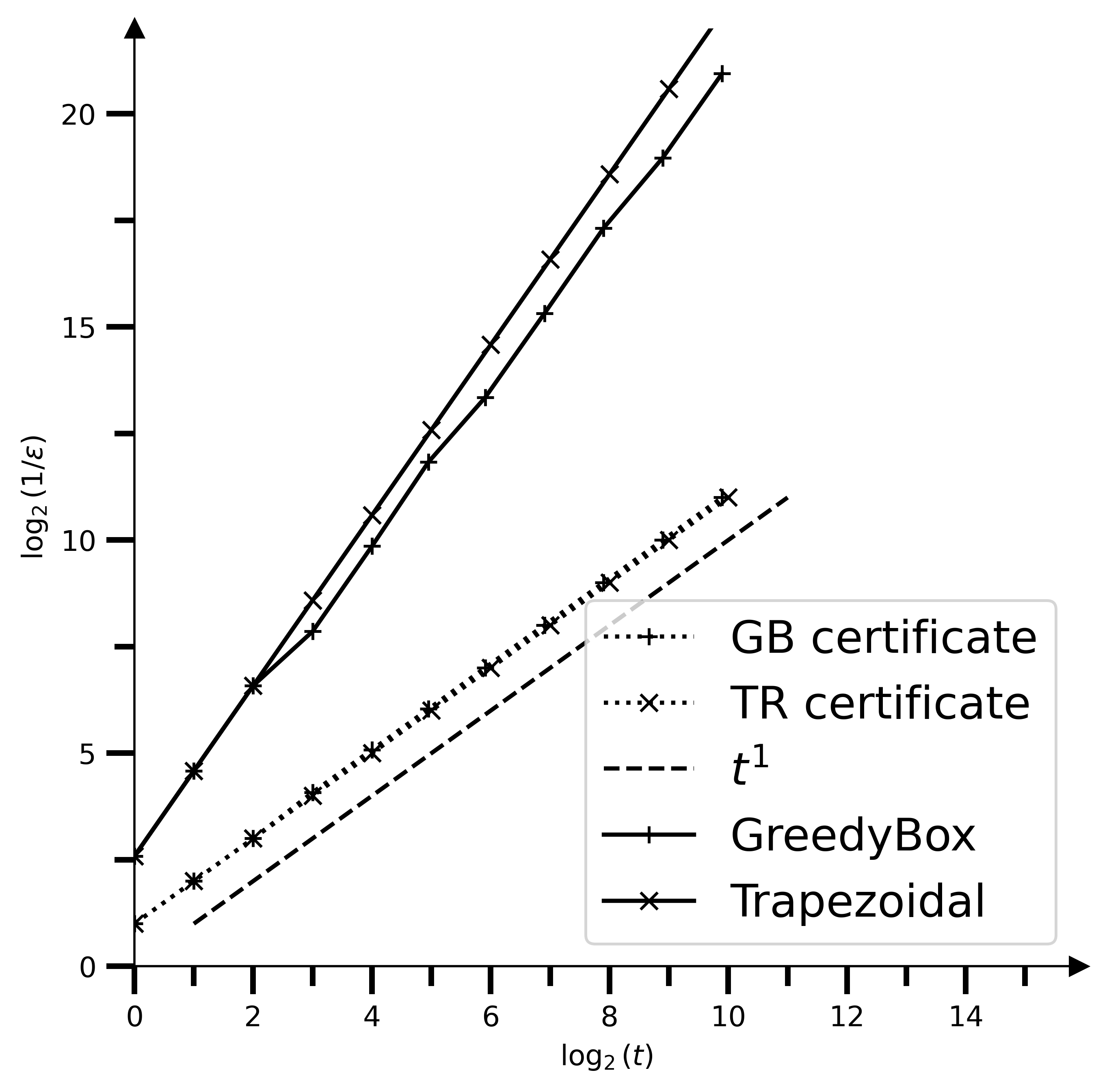
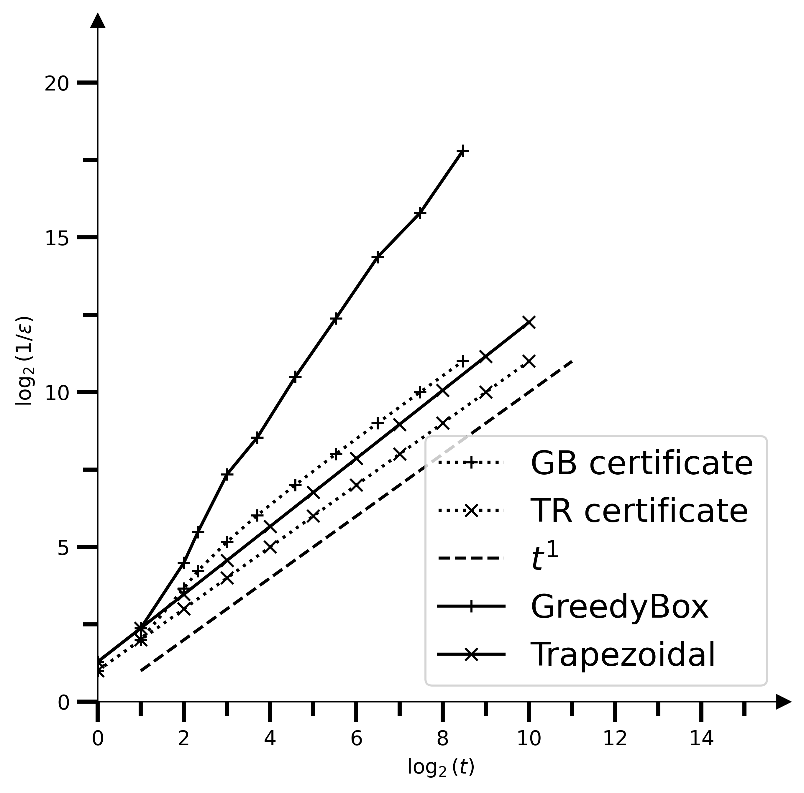
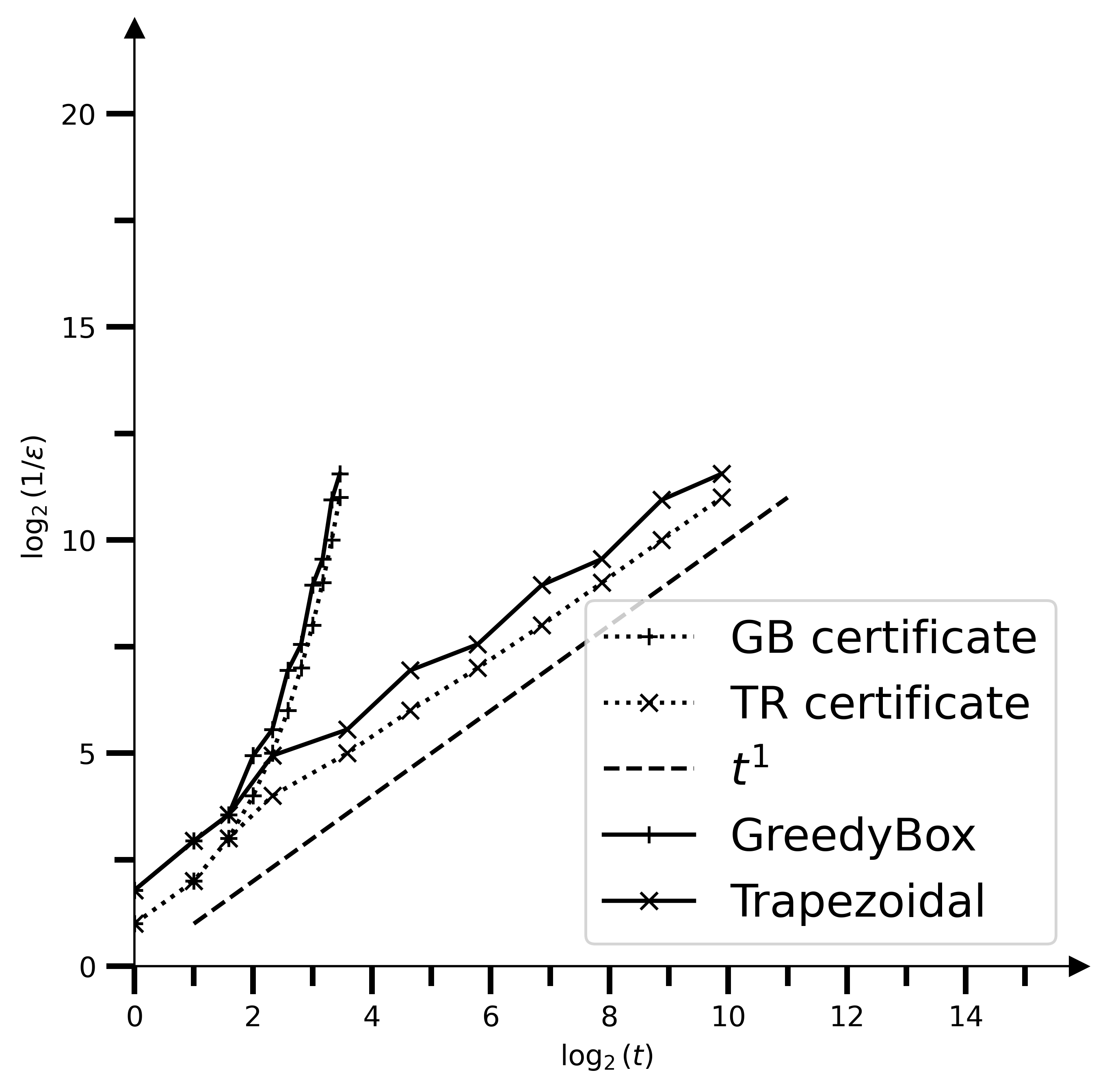
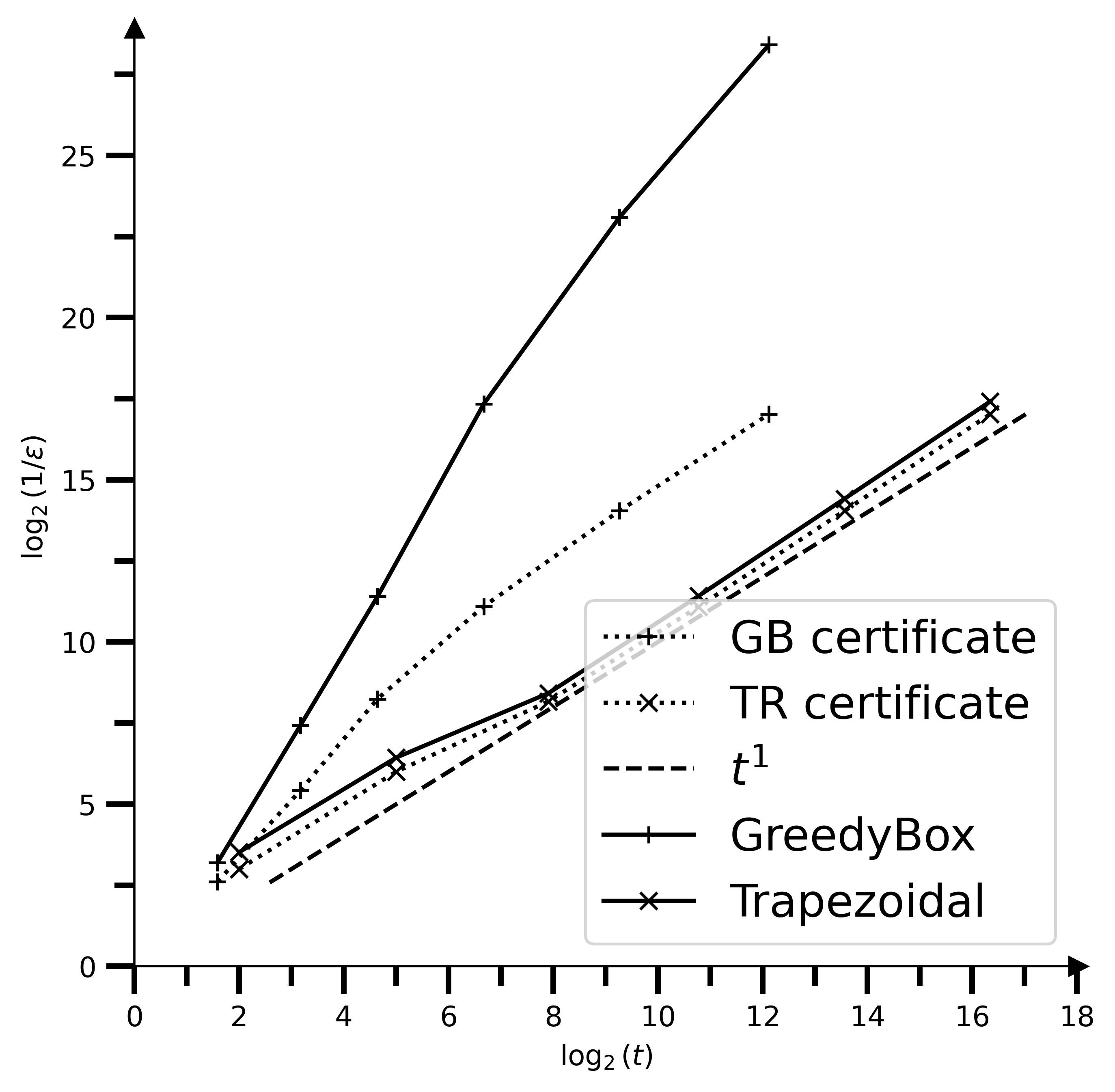
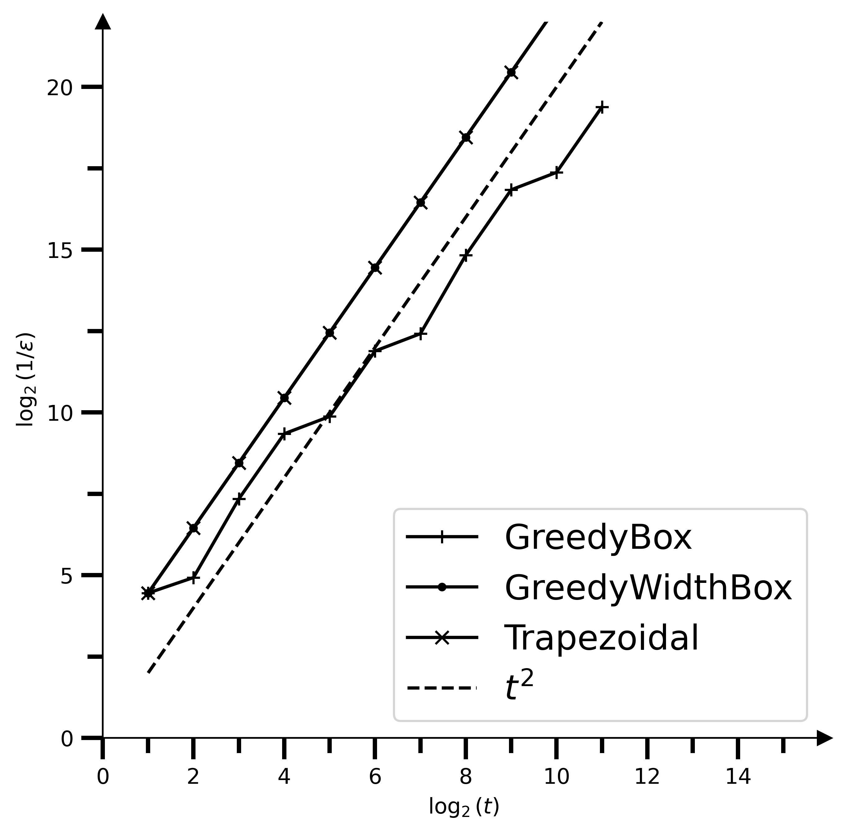
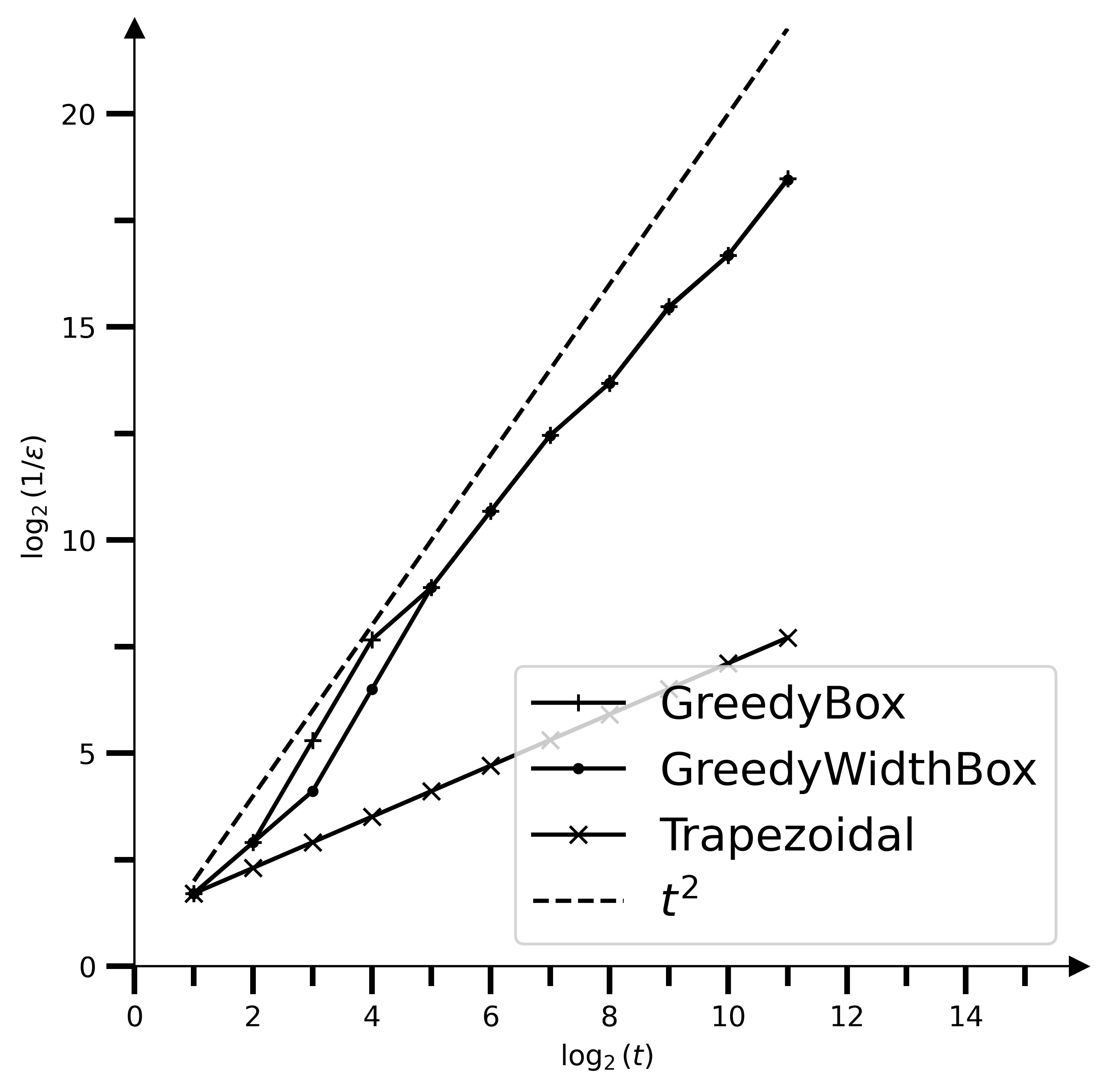
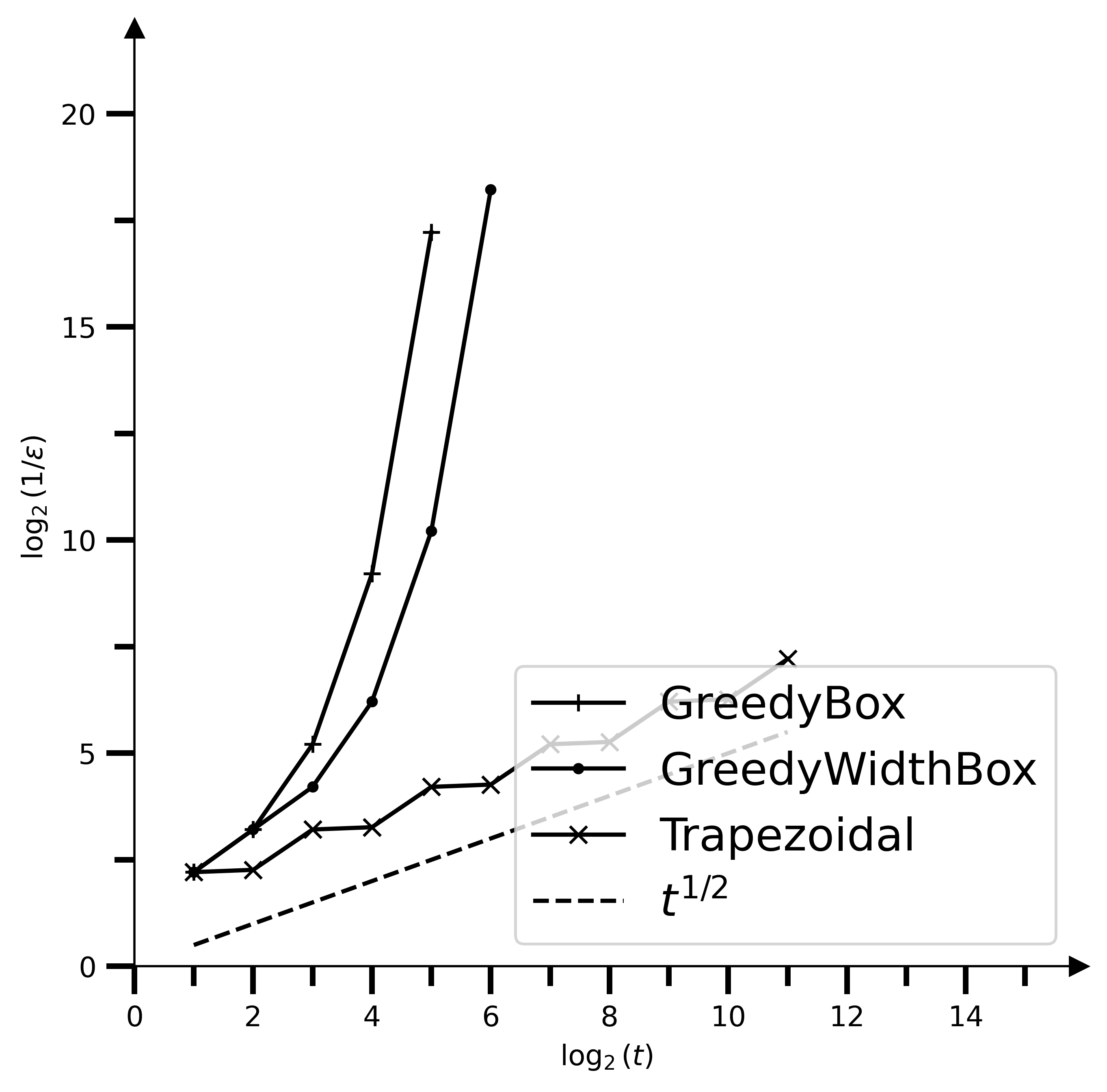
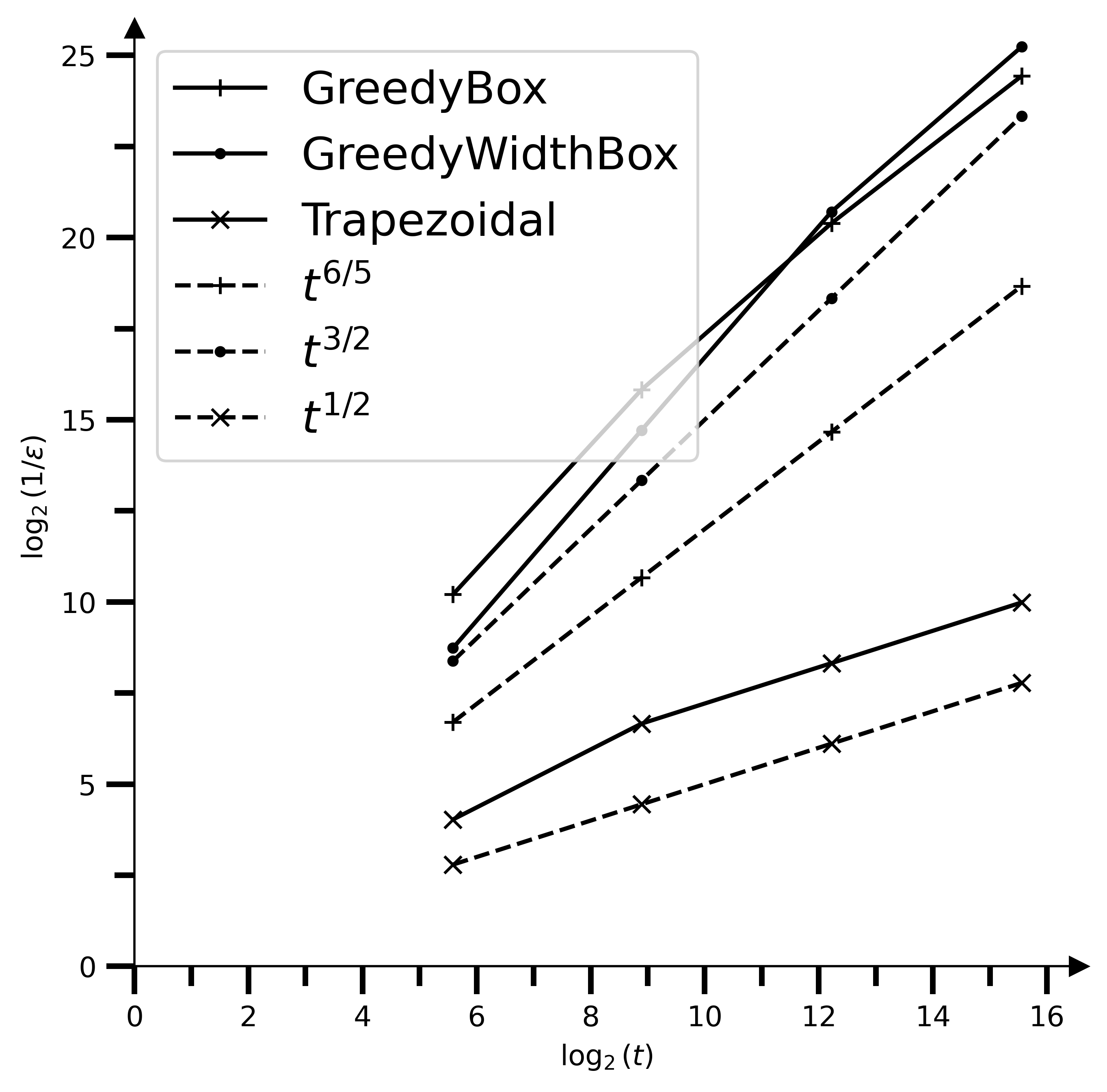
In order to have best-of-both-worlds theoretical results, we introduced a new algorithm called (Algorithm 3), which achieves the asymptotic rate for piecewise- functions, as soon as the number of pieces is finite. In Figure 4, we run the three algorithms for a fixed number of epochs, and observe the distance between the approximated function returned by the algorithm and the true function. Figures 4(a)-4(c) consider three different functions with various regularities. In Figure 4(d), we examine time-dependent piecewise- functions . Here, corresponds to the worst-case function as defined in (25) in the proof of Proposition 7, with an additional introduced discontinuity. For a better understanding of the results, we plot the inverse of this error, and plot everything with logarithmic scale. This means that a straight line with slope 1 represents a linear speed of convergence: an error that decreases inversely proportionally with the number of epochs. Figure 4(d) precisely confirms the anticipated worst-case rates as determined by the analysis for monotone piecewise- functions.
Remember however that given a desired precision , does not stop when its error is smaller than , but when its certificate (the best upper bound it can get without knowing a priori the function) is smaller than . Thus, for computation comparison, what really matters is to plot the convergence of the certificate with regard to some target error . The certificate of GreedyBox appears to be smaller than both GreedyWidthBox and the trapezoidal rule, regardless of the smoothness of the function. Yet, for most of the existing functions, the certificate of is of the order of . However, remark that the same bound apply both for the trapezoidal rule and for . This behavior can be seen on Figure 5 for GreedyBox and the trapezoidal rule. In Figure 5(d), we can see that GreedyBox provides certification of -accuracy approximately 30 times as fast as the trapezoidal rule. For functions, this certificate will never be a good upper bound of the real error, that often is of order for all three algorithms.
6 Conclusion and future works
In this paper, we studied the problem of approximating a non-decreasing function in norm, with sequential (adaptive) access to its values. We first proved an -dependent lower bound on the stopping time that holds for all algorithms with guaranteed error after stopping. We then presented the algorithm (inspired from Novak [1]) and showed that up to logarithmic factors, it is optimal among all such algorithms, for each non-decreasing function . As a direct consequence, we showed for the integral estimation problem that can be combined with additional randomization to get an improved rate in expectation. For the -approximation problem, we also investigated to what extent the error of can decrease faster (than guaranteed by the algorithm) for piecewise- functions. Put briefly, up to logarithmic factors, automatically achieves the improved (and optimal) rate of for a large number of singularities, , and a simple algorithmic variant () achieves this rate for any value of . In particular, our results highlight multiple performance gaps between adaptive and non-adaptive algorithms, and piecewise- functions, as well as monotone or non-monotone functions. We also provided numerical experiments to illustrate our theoretical results.
Several interesting questions about are left open. First, similarly to the faster rates proved for piecewise- functions, it would be interesting to investigate optimal rates for the average error, when is drawn at random from a probability distribution over the set of monotone functions (as, e.g., in Novak [1]). Second, for any fixed non-decreasing function , it would be useful to derive the limit (if any) of the empirical distribution of the points queried by . When and is the Lebesgue measure on , we conjecture that this limit exists and has a density roughly proportional to the square-root of the derivative of almost everywhere. Solving this problem would help complete our understanding of the behavior of , and of how it precisely adapts to the complexity of any function .
Several generalizations would also be worth investigating in the future. A seemingly straightforward direction is to work with Lipschitz functions on compact intervals; an algorithm defined similarly to but with parallelograms instead of rectangular boxes seems perfectly fit for this problem. Other natural directions consist in extending our -dependent bounds to multivariate monotone functions (in the spirit of, e.g., Papageorgiou [7]), to functions of known bounded variation, or variants of these function classes (e.g., entirely monotone functions, functions of bounded Hardy-Krause variation, see [29]).
Another natural and interesting research avenue is to address the case of noisy evaluations of . We believe that, under some known assumptions on the noise distribution, similar sample complexity guarantees (with slower rates) can be achieved by using a mini-batch variant of , which reduces the impact of noise by sampling multiple points and computing the average. Solving this problem would be a way to efficiently estimate cumulative distribution functions under a special censored feedback in the same spirit as in Abernethy et al. [30]. A variant of GreedyBox has been designed and analysed by [28] for addressing imperfect observations. However, the authors have solely established asymptotic convergence garantees (both point-wise and in terms of or norms) when the number of function evaluations approaches infinity, and they do not offer any guarantees regarding sample complexity.
7 Acknowledgements
The authors would like to thank Wouter Koolen for insightful discussions at the beginning of the work, as well as Peter Bartlett for fruitful feedback about improved rates for piecewise-regular functions. This work has benefited from the AI Interdisciplinary Institute ANITI, which is funded by the French “Investing for the Future – PIA3” program under the Grant agreement ANR-19-P3IA-0004. Sébastien Gerchinovitz and Étienne de Montbrun gratefully acknowledge the support of IRT Saint Exupéry and the DEEL project.999https://www.deel.ai/
Appendix A Elementary properties of box-covers
A.1 A general upper bound (proof of Lemma 1)
Lemma 1.
For all non-decreasing functions and , the quantity is well defined and upper bounded by
Proof.
Let . In order to prove the lemma, we exhibit a sequence of at most boxes, show that it is a box-cover of , and that the generalized areas of the boxes are such that .
For let . We also set . Note that . For , we define . Without loss of generality, we assume that for all . (Otherwise, we just remove all ’s such that , and remark below that the ’s still cover the graph of except maybe at the ’s.)
We start by showing that is a box-cover of . First, are adjacent boxes by construction. Note also that the graph of is included in the union of the ’s except maybe at the ’s. Indeed, for all and all , we have by definition of and , and by monotonicity of . Therefore, . This proves that is a box-cover of .
We are left to show that . We have
This entails that , which concludes the proof. ∎
A.2 Technical Lemmas on box-covers
We state here two elementary lemmas about box-covers. The first one below indicates that box-covers of with desired properties exist not only for (or ) but also for all larger values of .
Lemma 6.
Let and be any non-decreasing function. Then,
-
•
for all , there exists a box-cover of such that ;
-
•
for all , there exists a box-cover of such that for all .
Proof.
The proof of the two items is straightforward. For the first one, consider any box-cover of , with , such that . Then, split the last box vertically into sub-boxes . We can immediately see that
so that the sequence of boxes is a box-cover of with cardinality that satisfies the desired generalized area property. The second item can be proved similarly. ∎
The next simple lemma indicates that the values and in any box-cover of are necessary lower and upper bounds on the values of inside the boxes.
Lemma 7.
Let be non-decreasing, and be any box-cover of , with for all , for some sequence . Then, for all ,
Proof.
Let . Since and for any , we have and therefore
We conclude by taking the infimum or supremum over all and by using the fact that is non-decreasing. ∎
A.3 Relationship between and
In this section, we compare the two complexity quantities and defined in Section 1.2.
The quantity always satisfies . The next lemma relates the two complexity notions in a tighter way. Intuitively, if all the boxes of a minimal box-cover of satisfying had similar generalized areas , these areas would be close to , so that
The following lemma implies that indeed
up to a factor of .
Lemma 8.
Let and . Then,
In the proof of Theorem 2 we only use the first inequality . The second inequality shows that this step is tight up to a constant of .
Proof.
Let be a non-decreasing function and .
-
(a)
We prove that . For the sake of readability, we assume that is the Lebesgue measure on , and will explain at the end how to adapt the proof for an arbitrary probability measure . By and Lemma 6, there exists a box-cover of satisfying . Following a technique from Novak [1, Proof of Theorem 3], we now divide the ’s into as many sub-boxes as necessary so that each of their generalized areas is below . We will show that the overall number of resulting boxes is at most .
Let . We split the box in a vertical fashion by splitting into intervals of equal sizes , where . The choice of ensures that .
Then, we define the smaller boxes for . Their generalized areas are given by as required. Furthermore, the new total number of boxes is
Since contains the graph of except maybe at the ’s endpoints (and thus everywhere outside the ’s endpoints), we have shown that , as desired.
When is not the Lebesgue measure on , the proof can be slightly adapted as follows. For each box as above, we distinguish two cases.
Case 1: if , we set , , and as above.
Case 2: if , we set , , and as above. However, for any (if any), we take as a quantile of order of the conditional distribution . Then, among all sub-boxes , , we only keep the non-degenerate ones, i.e., those such that .The rest of the proof remains unchanged. In particular, each remaining sub-box satisfies , and the total number of sub-boxes is at most of .
-
(b)
Before proving the second inequality, we prove an intermediate result: for all , we have
(9) Since , we can consider a box-cover of with generalized areas at most of each. The result immediately follows from
-
(c)
We write for simplicity. We prove that by contradiction. Let us assume that and define
Then using Inequality (9), with substituted with , we get
which contradicts the assumption and thus proves the desired inequality.
∎
Appendix B Omitted proofs
B.1 Proof of Lemma 2
Lemma 2.
Let be non-decreasing, and . For any ,
Proof.
Remark that the approximation is the continuous piecewise-affine function such that for all . Therefore, it suffices to show that for each ,
which follows easily from the fact that on the -th box (since is non-decreasing), and by definition of . Summing over concludes the proof. ∎
As a supplement, we are left with proving the special case of the Lebesgue measure, for which the result holds with a multiplicative factor of .
Lemma 9.
Let be non-decreasing. At any round ,
Proof.
Summing over it suffices to show that for each ,
Let . To ease the notation, we make a change of variables and define for all :
We have
The function is non-decreasing over with and . It remains to control by . which is done in the following.
First we remark that we can assume . Otherwise, since is non-decreasing for all and , which concludes.
We consider the two points such that the sign of does not change over . More formally, they are defined as:
and
Note that the sign of is constant over since . Now, we show the following two facts
| (10) |
Indeed, let , by definition of , it exists such that
and thus using again the definition of for all , If , we are done since because is non-decreasing and . Otherwise using , and making concludes the first inequality of (10). The second inequality can be proved similarly.
B.2 Proof of Lemma 3
Lemma 3.
Let be non-decreasing, and . Define , and assume that is such that . Then, at time , all the boxes maintained by have a generalized area bounded from above by , i.e., for all .
Proof.
By definition of , we can fix a box-cover of such that for all . Recall that these boxes are adjacent, i.e., they are of the form for some nodes . The inequalities thus translate into for all .
In this proof we will compare the boxes maintained by with the boxes above. We first need the following definition: at each round , we say that a box , , maintained by is
-
•
internal if for some ;
-
•
overlapping if for some .
Note that exactly one of the two cases above must hold true. In the sequel, we denote by the box selected by at time . Since is necessary of one of the two types above, we can distinguish between the following two cases.
Case 1: there exists such that is internal. In this case, letting be the corresponding index, we have, by Lemma 7 in Appendix A.2,
Therefore, the generalized areas of and satisfy by construction of . Now, by definition of in Algorithm 1:
This concludes the proof of the lemma in this case, since the quantity can only decrease between rounds and .
Case 2: is an overlapping box at every round . In this case, we say that all nodes lying in are activated at time . More precisely, we say that a node is left-activated when (part of the box lies on the left of ), and that it is right-activated when (part of the box lies on the right of ).
Since by construction, at least one node is either left-activated or right-activated at every round , so that
Inverting sums and recognizing to be the number of rounds when node is -activated, we can see that
so that
Combining the last inequality with the definition of and , we obtain the following intermediate result.
Fact 1.
There exists and such that the node is -activated at least
times within the set of rounds .
We now focus on a single pair provided by Fact 1 above. We follow the evolution of the box maintained by that lies on the -side of . More formally, if we write , this means that if , and that if . Note that, at any round , such a box indeed exists and is unique.
Note that, at all rounds when is -activated, we have , so that the box is replaced (see Step 3 in Algorithm 1) by two boxes whose generalized widths are at most half that of . This is because is a median of the conditional distribution . Since is among these two boxes, we thus have
at each round when is -activated. Note also that at all other rounds ; at such rounds, . Combining the last two properties, and denoting by the round when is -activated for the -th time, we get
To conclude, denote by the round when is -activated for the -th time. Note that so that
where the first inequality follows from and the fact that is non-increasing over time. Therefore, by definition of , all boxes maintained by at time have generalized areas bounded by
We conclude the proof by noting that , so that . ∎
B.3 Proof of Lemma 4
Lemma 4.
Let be non-decreasing, and . For any , we have . Therefore, for all in ,
Proof.
We first prove that for all . To do so, recall that at any round , maintains boxes given by , . We write for their generalized areas sorted in decreasing order.
Part 1: We first show by induction on that
- (i)
-
(ii)
at least boxes of round are identical to boxes of round .
Both (i) and (ii) are straightforward for . Assume they are true for some . Next we prove (i) and (ii) with the index value . At round , the generalized area of the box selected by must be at least as large as the maximum generalized area of the boxes that are identical to boxes of round (by (ii) with ). Therefore, this generalized area is larger than or equal to , which proves (i). Property (ii) is immediate since only one box is selected at every round. This completes the induction.
Part 2: Note that, at each round , the box selected by is replaced with two smaller boxes and whose generalized areas satisfy
since is a median of and for any . Therefore, and by Property (i) above, at least is lost when summing the generalized areas to the power at round , compared to round . Therefore, the certificate of the box-cover at the next round satisfies . Summing over we get:
To see why this implies (5), it suffices to note that , so that
where the first inequality is because the certificate can only decrease over time, and where the last inequality follows from the property shown above. This concludes the proof. ∎
B.4 Proof of Theorem 4
Theorem 4.
Proof.
Let . First, we remark that the points defined by the deterministic version (defined in Algorithm 1) and the stochastic version (Algorithm 2) are identical. Only the stopping criterion and definition of differs from Algorithm 1. Therefore, we can apply Lemma 3.
Let that will be fixed later as a function of . Denote by Assumption 1. Applying Lemma 3 to , we get the following result. At time
all the boxes maintained by Algorithm 2 have an area bounded from above by , i.e.,
From Lemma 8 since by Assumption 1,
which substituted into the definition of yields
Thus, the certificate up to time is bounded from above as
Now, to get rid of the multiplicative term, similarly to Theorem 2, we can apply Lemma 4 (which also works for StochasticGreedyBox) to replace with for . The choice yields
Then, choosing implies . Therefore by definition of the stopping criterion
This concludes the proof. ∎
B.5 Proof of Theorem 5
Theorem 5.
Let and . Let be a non-decreasing and piecewise- function with a number of -singularities bounded by and such that whenever it is defined. Then, there exists
such that for all , where is the approximation of returned by after rounds.
Proof.
Let , and be two constants to be fixed later by the analysis and set .
Step 1. We will now establish an upper bound on the number of evaluations, denoted by , required by GreedyBox to ensure that all individual areas are smaller than . From Lemma 3, we know that
| (13) |
which can be further bounded from above by the use of Lemma 8 in the appendix with the choice . Indeed, since and by Lemma 1, . Thus, Lemma 8 entails
Therefore, plugging back into Inequality (13), the number of required evaluations is bounded as
| (14) |
Step 2. We will now fix the values of and in a way that ensures an approximation error in the -norm smaller than .
For , let us denote by the box maintained by , define to be the width of the box and let be the piecewise-linear function returned by after epochs. By the first step of this proof, for all ,
which implies by construction of (see Proof of Lemma 2), for all
| (15) |
The remaining part of the proof revolves around using the above upper bound for the non-smooth pieces and a more refined upper bound for the pieces. Denote by the indices of all boxes such that is over . Because is piecewise- with at most pieces, . Therefore, the error after evaluations may be decomposed as
| (16) |
We are now left with bounding from above the errors on the right-hand-side for all . On one side, the bound (15) is valid for all , which we bound further by . On the other side, we can use Lemma 11 that bounds the approximation error of for any and piecewise- function to obtain
| (17) |
where , where denotes the set of -singularities. This prompt us to introduce the following function , that depends on the width of the intervals of :
From (16), the total error is thus bounded from above by
| (18) |
It now remains to bound the function for any set of possible widths that could arise from . We thus need to solve the maximization problem
may be re-written in two terms:
| (19) |
Let us first handle the first term. Since , we have in particular
This shows that the number of intervals in the first term verifies
| (20) |
which implies that the first term of (19) is bounded as
| (21) |
Now, let us bound from above the second term of the sum. Since is strictly convex on , Lemma 10 (in the appendix) applied with and states that the second term of (19) is bounded in the following way:
| (22) |
Substituting the two upper bounds (21) and (22) into (19), we have
which substituted into (18) yields
| (23) |
Now, we finalize the proof by considering three cases depending on the value of and by optimizing and for each situation.
Case 1: . Then, , which substituted in (23), implies
Choosing yields
The choice implies for
and by (14), the number of required evaluations is of order
which concludes the first statement of the theorem.
Case 2: . Then, one may then use Theorem 2, which does note use the piecewise-regularity assumption of , and implies that for with
B.6 Proof of Proposition 6
Proposition 6.
Let , and . Then, for any deterministic adaptive algorithm and for any
there exists a non-decreasing piecewise-affine function with at most discontinuities, such that .
Proof.
Let , and . Let be an adaptive algorithm and fix a number of evaluations. We aim to design a function with at most discontinuities such that if is sufficiently small.
Let be the identity function on . Let and and denote by the points that the algorithm would have chosen after evaluations, if it was applied on and by its estimation. Then, we define two functions and such that
Let . For , we define the width of the -th interval. Let denotes the set of indexes that correspond to the largest intervals (i.e., such that for all and and ). Then, we define for all
and
Then, and have at most discontinuities and are such that for all . Thus, since is deterministic, the function estimation and the points chosen by on and after evaluations would also respectively be and .
Furthermore, we have
By triangular inequality, this yields
Therefore, if
which, using , is satisfied for
Noting that and have at most discontinuities and that elsewhere concludes the proof. ∎
B.7 Proof of Proposition 7
Proposition 7.
Let . Then, there exists piecewise- function with one -singularity, such that there exists with where is the approximation at evaluations.
Proof.
Let that will be chosen later by the analysis. Set , and .
Step 1. Design of a worst-case function We will design a worst-case function that will cause GreedyBox to incur a large -error after iterations. The function will consist of two components: one for that oscillates with a second derivative , and another that is linear for . has a continuous derivative and its second derivative is piecewise-continuous wit singularities. An illustration is given in Figure 2 for ().
Let us first design the first oscillating part, that we call , and is defined recursively for all by
| (24) |
Then, we define by: for all
| (25) |
Step 2. Expression of the approximation provided by GreedyBox after iterations on . Let us understand how behaves during the first iterations when given this function. Once done, we will be able to retrieve the expression of the approximation of made by .
Remark that for , (during the first oscillating part), the area of the box is
Similarly, for , (during the linear part), the area of the box is
Thus, because tends to equalize the areas of the different boxes, and because it maintains areas of the form for some in and (it can only splits intervals in ), the box cover we just described is a potential output of after epochs.
Let us formally prove that it is precisely the case. For any and , the area of the box is . Likewise, for any and , the area of the box is . Thus, if for some epoch , one box on the left of has a width greater than , its area will be greater than or equal to , and if one box on the right of has a width greater than , its area will be greater than or equal to . In both cases, the area is strictly greater than , and would choose at Line 1 to split this box rather than any other box that already has area .
Splitting one by one boxes with area greater than , obtains at time the boxes with exact area described previously. is the linear interpolation between all the points where is the extremity of one of the box.
Step 3. Error of GreedyBox on after iterations. Now that we exhibited the exact value of , we are left with computing the total error made by on after steps. Since is linear on the interval , equals on this segment. Then,
Step 4. Choice of . We are left with choosing as large as possible such that the above error is at least . That is,
which can be rewritten as
Thus choosing , yields
Note that the designed function has a number of -singularities
but only has one -singularity at . This concludes the proof. ∎
B.8 Technical lemmas for regular functions
In this section, we establish two technical lemmas that are used in our analysis of GreedyBox for piecewise- functions. The first lemma, presented below, is a property of strictly convex functions.
Lemma 10.
Let , , and be a strictly convex function on . Then
and the maximum is reached for , , , where .
Proof.
Let be as in the statement of the theorem, and let us show that it is optimal. Let be a real-number. Since only the sum of the matters, we can assume without loss of generality that the ’s are sorted in decreasing order. Now, assume that , and let us show that is not a maximum.
Because the sum of the ’s still needs to be equal to , either , or . Assume first that . Furthermore, assume that . This means that is closer to than is from . Let , and . Then,
Then for , and for , , which shows that is suboptimal. We can do the same kind of construction when or when . All these different cases show that is maximized only when the largest possible amount of the ’s are at the extremity of the constraint set, that is when or . This concludes the proof. ∎
The second technical Lemma below recalls a classical result and provides an upper bound on the -error achieved by an affine approximation of a function. In particular, this lemma implies a sample complexity of order for the trapezoidal rule to provide an -approximation in norm for functions.
Lemma 11.
Let . Assume that is and piecewise- and such that for all where it is defined. Then,
where is the affine approximation defined for all by:
Proof.
Since is piecewise- with bounded second derivative, is absolutely continuous, we can thus apply the Taylor-Lagrange Theorem with the integral form of the remainder with . We have for all
We now control the -error of . The above inequality yields that for all there exists such that and
Thus, applying it with entails
which in turns implies that
Therefore, with the change of variable , we get
which concludes the proof. ∎
Appendix C Numerical experiments: the -norm case
In the core of the paper, we gave some plots on the error of , and as compared to the trapezoidal rule in Section 5. In this section, we complete the comparison by displaying some plots for the -norm. In this case, the area of a box is worth .
We can notice several interesting facts on the plots of Figure 6. First, the trapezoidal rule, and behaves better than for the square function. This is the first case we could find where the trapezoidal rule has a better speed of convergence than . Another point is that on Figure 6(b), the trapezoidal rule has a bound of order . However, in Theorem 2, we proved that has an error at worst of the order of , which we proved to be smaller than . Yet, for this example, the trapezoidal does not converge in , which proves that satisfies better worst case property than the trapezoidal rule for -norm with . Figure 6(c) shows results similar to the -norm. In, Figure 6(d), we consider the for approximating , where is the function defined in equation (25) at . The empirical rates seem to confirm once again the anticipated worst-case rates as determined by our analysis.
References
- \bibcommenthead
- Novak [1992] Novak, E.: Quadrature formulas for monotone functions. Proceedings of the American Mathematical Society 115(1), 59–68 (1992)
- Davis and Rabinowitz [1984] Davis, P.J., Rabinowitz, P.: Methods of Numerical Integration. Elsevier Science, Netherlands (1984)
- van der Vaart [1998] Vaart, A.W.: Asymptotic Statistics. Cambridge Series in Statistical and Probabilistic Mathematics. Cambridge University Press, Cambridge (1998)
- Sukharev [1986] Sukharev, A.G.: On the existence of optimal affine methods for approximating linear functionals. Journal of Complexity 2(4), 317–322 (1986)
- Bakhvalov [1971] Bakhvalov, N.S.: On the optimality of linear methods for operator approximation in convex classes of functions. USSR Computational Mathematics and Mathematical Physics 11(4), 244–249 (1971)
- Kiefer [1957] Kiefer, J.: Optimum sequential search and approximation methods under minimum regularity assumptions. Journal of the Society for Industrial and Applied Mathematics 5(3), 105–136 (1957)
- Papageorgiou [1993] Papageorgiou, A.: Integration of monotone functions of several variables. Journal of Complexity 9(2), 252–268 (1993)
- Brass and Petras [2011] Brass, H., Petras, K.: Quadrature Theory: the Theory of Numerical Integration on a Compact Interval. Mathematical Surveys and Monographs, vol. 178. American Mathematical Soc., Rhode Island, USA (2011)
- Novak and Roschmann [1996] Novak, E., Roschmann, I.: Numerical integration of peak functions. Journal of Complexity 12(4), 358–379 (1996)
- Graf and Novak [1990] Graf, S., Novak, E.: The average error of quadrature formulas for functions of bounded variation. The Rocky Mountain journal of mathematics 20(3), 707–716 (1990)
- Novak [1993] Novak, E.: Quadrature formulas for convex classes of functions. In: Numerical Integration IV: Proceedings of the Conference at the Mathematical Research Institute, Oberwolfach, November 8–14, 1992, pp. 283–296 (1993). Springer
- Novak [1995] Novak, E.: Optimal recovery and n-widths for convex classes of functions. Journal of Approximation Theory 80(3), 390–408 (1995)
- Hinrichs et al. [2011] Hinrichs, A., Novak, E., Woźniakowski, H.: The curse of dimensionality for the class of monotone functions and for the class of convex functions. Journal of Approximation Theory 163(8), 955–965 (2011)
- Ritter et al. [1993] Ritter, K., Wasilkowski, G.W., Woźniakowski, H.: On multivariate integration for stochastic processes. In: Numerical Integration IV: Proceedings of the Conference at the Mathematical Research Institute, Oberwolfach, November 8–14, 1992, pp. 331–347 (1993). Springer
- Katscher et al. [1996] Katscher, C., Novak, E., Petras, K.: Quadrature formulas for multivariate convex functions. Journal of Complexity 12(1), 5–16 (1996)
- Krieg and Novak [2017] Krieg, D., Novak, E.: A universal algorithm for multivariate integration. Foundations of Computational Mathematics 17, 895–916 (2017)
- Chandra [2002] Chandra, P.: Trigonometric approximation of functions in Lp-norm. Journal of Mathematical Analysis and Applications 275(1), 13–26 (2002)
- Fletcher et al. [1971] Fletcher, R., Grant, J., Hebden, M.: The calculation of linear best Lp approximations. The Computer Journal 14(3), 276–279 (1971)
- Fletcher et al. [1974] Fletcher, R., Grant, J., Hebden, M.: Linear minimax approximation as the limit of best l_p-approximation. SIAM Journal on Numerical Analysis 11(1), 123–136 (1974)
- Plaskota and Wasilkowski [2005] Plaskota, L., Wasilkowski, G.W.: Adaption allows efficient integration of functions with unknown singularities. Numerische Mathematik 102, 123–144 (2005)
- Plaskota et al. [2008] Plaskota, L., Wasilkowski, G., Zhao, Y.: The power of adaption for approximating functions with singularities. Mathematics of computation 77(264), 2309–2338 (2008)
- Kopotun and Shadrin [2003] Kopotun, K., Shadrin, A.: On k-monotone approximation by free knot splines. SIAM journal on mathematical analysis 34(4), 901–924 (2003)
- Kopotun et al. [2009] Kopotun, K.A., Leviatan, D., Prymak, A.: Nearly monotone and nearly convex approximation by smooth splines in Lp, p striclty greater than 0. Journal of Approximation Theory 160(1-2), 103–112 (2009)
- Novak [1996] Novak, E.: On the power of adaption. Journal of Complexity 12(3), 199–237 (1996)
- Lattimore and Szepesvári [2020] Lattimore, T., Szepesvári, C.: Bandit Algorithms. Cambridge University Press, Cambridge (2020)
- Jones et al. [1998] Jones, D.R., Schonlau, M., Welch, W.J.: Efficient global optimization of expensive black-box functions. Journal of Global optimization 13, 455–492 (1998)
- Bachoc et al. [2021] Bachoc, F., Cesari, T., Gerchinovitz, S.: Instance-dependent bounds for zeroth-order lipschitz optimization with error certificates. Advances in Neural Information Processing Systems 34, 24180–24192 (2021)
- Bonnet et al. [2020] Bonnet, L., Akian, J.-L., Savin, É., Sullivan, T.J.: Adaptive reconstruction of imperfectly observed monotone functions, with applications to uncertainty quantification. Algorithms 13(8), 196 (2020)
- Fang et al. [2021] Fang, B., Guntuboyina, A., Sen, B.: Multivariate extensions of isotonic regression and total variation denoising via entire monotonicity and Hardy-Krause variation. The Annals of Statistics 49(2), 769–792 (2021)
- Abernethy et al. [2016] Abernethy, J.D., Amin, K., Zhu, R.: Threshold bandits, with and without censored feedback. Advances in Neural Information Processing Systems 29 (2016)