A Multi-scale Generalized Shrinkage Threshold Network for Image Blind Deblurring in Remote Sensing

Abstract

Remote sensing images are essential for many earth science applications, but their quality can be degraded due to limitations in sensor technology and complex imaging environments. To address this, various remote sensing image deblurring methods have been developed to restore sharp, high-quality images from degraded observational data. However, most traditional model-based deblurring methods usually require predefined hand-craft prior assumptions, which are difficult to handle in complex applications, and most deep learning-based deblurring methods are designed as a black box, lacking transparency and interpretability. In this work, we propose a novel blind deblurring learning framework based on alternating iterations of shrinkage thresholds, alternately updating blurring kernels and images, with the theoretical foundation of network design. Additionally, we propose a learnable blur kernel proximal mapping module to improve the blur kernel evaluation in the kernel domain. Then, we proposed a deep proximal mapping module in the image domain, which combines a generalized shrinkage threshold operator and a multi-scale prior feature extraction block. This module also introduces an attention mechanism to adaptively adjust the prior importance, thus avoiding the drawbacks of hand-crafted image prior terms. Thus, a novel multi-scale generalized shrinkage threshold network (MGSTNet) is designed to specifically focus on learning deep geometric prior features to enhance image restoration. Experiments demonstrate the superiority of our MGSTNet framework on remote sensing image datasets compared to existing deblurring methods.

I Introduction

Recently, with the rapid advancement of remote sensing technology, remote sensing images have been used in a variety of applications, such as object detection[1, 2, 3], scene segmentation[4, 5, 6], and remote sensing image fusion[7, 8, 9]. However, the quality of these images is often compromised due to the constraints of the imaging hardware and the intricate imaging environment. This has a direct impact on the performance of algorithms in various fields. To address this, the most cost-effective solution is to use image deblurring techniques. These techniques can restore images to a higher quality with more distinct details than their low-quality counterparts, without the need to upgrade the equipment. This has made image deblurring a popular topic in the fields of remote sensing and computer vision.

The classical image degradation model can be expressed mathematically as follow:

$$\mathbf{g}=\mathbf{h}\ast\mathbf{u}+\mathbf{n},$$ (1)

where $\mathbf{g}$ is the degraded observed image, $\mathbf{u}$ is the latent image with sharp details, $\mathbf{h}$ is the blur kernel, $\mathbf{n}$ is the additive white Gaussian noise (AWGN), and ”$*$” denotes the two-dimensional convolution operator.

Attempting to restore the latent sharp image $\mathbf{u}$ and the blur kernel $\mathbf{h}$ from the observed degraded image $\mathbf{g}$, image blind deblurring is an ill-posed inverse problem due to the fact that equation (1) has many blur kernel/high-quality image pairs that do not guarantee a unique solution. To restrict the solution space, various image deblurring techniques have been explored, which can be divided into two categories: traditional model-based methods and deep learning-based methods.

Model-based methods typically involve the selection or construction of geometric prior terms as a primary means of addressing the deblurring problem. Researchers have developed a variety of geometric priors, such as self-similar priors [10, 11], total variational prior (TV) [12], gradient priors [13, 14], sparse coding priors [15, 16, 17], hyper-Laplacian prior [18], and dark channel prior [19]. These priors are used to determine the solution space for latent sharp images and blur kernels.

Despite the success of traditional model-based image deblurring techniques, there are still some issues that have yet to be addressed. The priors used in these methods are typically designed manually, which can lead to an imprecise representation of both the sharp images and the blurred kernels. Furthermore, it can be challenging to select the appropriate parameters for these algorithms, and the computational complexity of solving the models is quite high, resulting in a longer algorithm execution time.

Deep learning-based image deblurring techniques typically employ an end-to-end network architecture to learn the intricate relationship between blur kernel/sharp image pairs [20, 21, 22]. Nah et al. [23] first introduced DeepDeblur, a network that can directly restore sharp images from blurred images in an end-to-end framework. Deepdeblur gradually restores sharp images from coarse to fine through a cascade of sub-networks. Kupyn et al. [24, 25] presented image deblurring in the form of generative adversarial networks. Zhang et al. [26] proposed the residual dense block (RDB) and the residual dense network (RDN) for image restoration. Mao et al. [27] suggested a residual module for the frequency domain that extracts information from the frequency domain to achieve a balance between high-frequency and low-frequency information. Cui et al. [28] presented an image restoration framework denoted as a selective frequency network (SFNet), which is built on a frequency selection mechanism. Cho et al. [29] revisited the coarse-to-fine strategy and presented a multi-input and multi-output U-net (MIMO-UNet) for single image deblurring.

Recently, some deep learning-based methods have incorporated deep networks into classic model-based optimization algorithms and proposed end-to-end deep unfolding networks with optimized parameters [30, 31, 32, 33, 34, 35, 36, 37, 38]. Quan et al. [30] proposed an unfolding deblurring network based on a Gaussian kernel mixture model and a fixed-point iteration framework. Xu et al. [31] proposed a new paradigm that combined deep unfolding and panchromatic sharpening observation models. Li et al. [32] proposed a deep unfolding method for blind deblurring based on a generalized TV regularization algorithm. Zhang and You [33, 34] proposed ISTA-Net, ISTA-Net + and ISTA-Net ++ for image compressive sensing (CS) reconstruction based on the Iterative Shrinkage-Thresholding Algorithm (ISTA). Fan et al. [39] proposed a deep geometric incremental learning framework based on second Nesterov proximal gradient optimization. Inspired by the physical principles of the heat diffusion equations, Cui et al.[40] developed an interpretable diffusion learning MRI reconstruction framework that combines k-space interpolation techniques and image domain methods.

Investigations have shown that deep learning-based approaches are effective in image deblurring. However, there are still some challenges that need to be addressed [41, 42]. Most deep learning networks do not take into account prior knowledge of the image. Additionally, the end-to-end black-box design of the deep learning network makes it difficult to analyze the role of the network architecture. MAP-based deblurring technology is based on Equation (1) to generate satisfactory results. Therefore, it is essential to incorporate an image statistical inference model into the network architecture to improve image deblurring performance. Several deep unfolding networks use a basic convolution layer to learn the priors of the image. Nevertheless, a more complex network structure should be used to capture the complex image prior.

To solve the above problems, this paper proposes a novel approach for image blind deblurring that utilizes multi-scale deep prior learning. The blur kernel and latent sharp image are initially learned through a linear reconstruction step, followed by a deep learning module to capture the deep prior features of the image/blur kernel. Furthermore, a multi-scale generalized shrinkage thresholding technique is proposed to restore lost texture details and improve the restoration of finer image details. The main contributions of this work are summarized as follows:

• A MAP-based multi-scale generalized shrinkage threshold network to solve the blind deblurring problem of images is proposed, leading to an end-to-end trainable and also interpretable framework (MGSTNet);

• We design a proximal-point mapping module that can be learned in the blur kernel reconstruction step. This module is able to learn and filter deep prior information of the blur kernel, resulting in a significant improvement in the evaluation of the blur kernel.

• We create an image deep proximal mapping module that combines a generalized shrinkage threshold operator and a multi-scale prior feature extraction block. Additionally, we incorporate an attention mechanism to adaptively adjust the importance of the prior, thus avoiding the disadvantages of hand-crafted image prior terms.

• The experiments demonstrate that the proposed MGSTNet framework yields superior image restoration quality for blurred images with varying levels of deterioration.

The remainder of this paper is organized as follows. Section II introduces the proposed MAP-based multi-scale generalized shrinkage threshold network for image blind eeblurring in remote sensing, and the experimental results are analyzed in Section III. Conclusions are presented in Section IV.

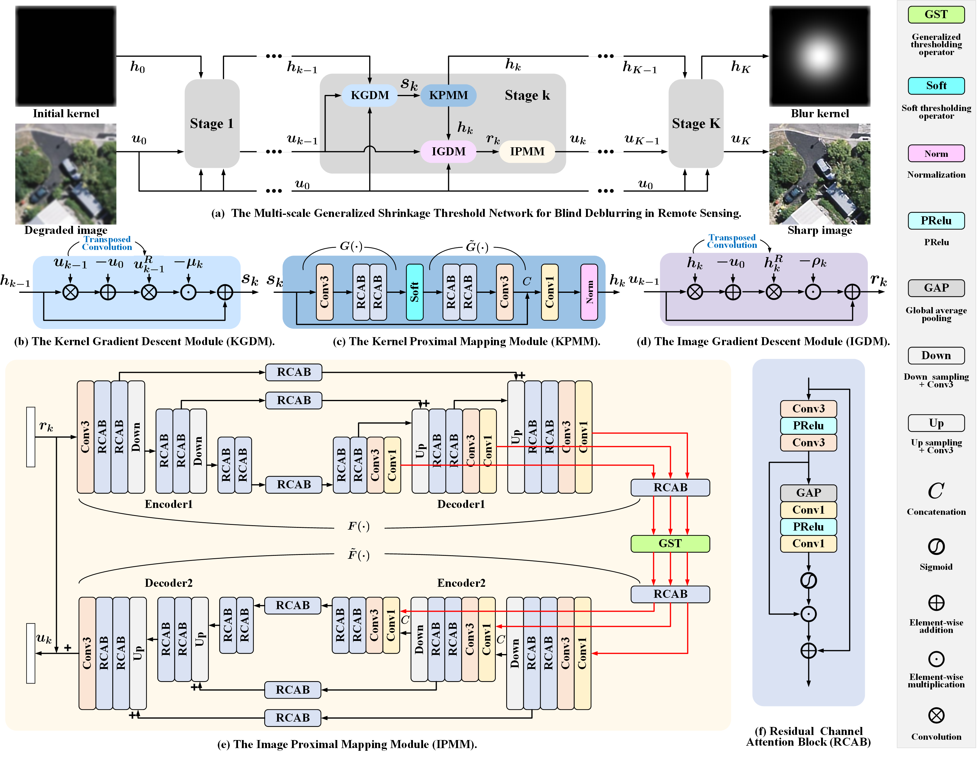
Figure 1: The overall framework of the proposed MGSTNet that learns enriched feature representations for image blind deblurring. MGSTNet is based on an iterative design with alternating image/blur kernel optimization, and its main idea is to learn the representation mapping between the image space (or kernel space) and the feature space by using an encoder-decoder module and a shrinkage threshold module.

II Methodology

II-A The Maximum A Posteriori Framework

The Maximum A Posteriori (MAP) is a powerful tool for solving inverse problems. It is based on Bayesian inference and provides a systematic way to regularize solutions from a set of observations. It is particularly useful for ill-posed problems in image processing, where the image restoration solution is not unique. To better understand our work, we will provide a brief overview of the MAP framework used in blind deblurring methods [21, 22], i.e, estimating the image $\mathbf{u}$ and the blur kernel $\mathbf{h}$ from a given blurred image $\mathbf{g}$, which is defined as follows:

$$\begin{split}(\mathbf{u},\mathbf{h})&=\underset{\mathbf{u},\mathbf{h}}{\operatorname{argmax}}\enspace p(\mathbf{h},\mathbf{u}\mid\mathbf{g})\\ &=\underset{\mathbf{u},\mathbf{h}}{\operatorname{argmax}}\enspace p(\mathbf{g}\mid\mathbf{h},\mathbf{u})p_{u}(\mathbf{u})p_{h}(\mathbf{h}),\end{split}$$ (2)

where $p(\mathbf{h},\mathbf{u}\mid\mathbf{g})$ is the posterior probability, $p(\mathbf{g}\mid\mathbf{h},\mathbf{u})$ represents the likelihood function. The $p_{u}(\mathbf{u})$ and $p_{h}(\mathbf{h})$ denote the probability density functions (statistical priors) of $\mathbf{u}$ and $\mathbf{h}$, respectively.

According to (1) and the general formulation of MAP-based blind deblurring, we define the likelihood probability term as

$$p(\mathbf{g}\mid\mathbf{h},\mathbf{u})\propto e^{-\cfrac{\|\mathbf{h}\ast\mathbf{u}-\mathbf{g}\|_{2}^{2}}{2\sigma^{2}}}$$ (3)

and further define the two prior probability terms as follows

$$\begin{split}p_{u}(\mathbf{u})\propto e^{-\cfrac{\|\Psi(\mathbf{u})\|_{p}^{p}}{2\sigma^{2}}},\quad p_{h}(\mathbf{h})\propto e^{-\cfrac{\|\Phi(\mathbf{h})\|_{1}^{1}}{2\sigma^{2}}}.\end{split}$$ (4)

Taking the negative logarithm of both sides of (2) yields a MAP estimator, which is expressed as follows:

$$\underset{\mathbf{u},\mathbf{h}}{\operatorname{argmin}}-\log p(\mathbf{g}\mid\mathbf{h},\mathbf{u})-\log p_{u}(\mathbf{u})-\log p_{h}(\mathbf{h}),$$ (5)

where $\log\;p_{u}(\mathbf{u})$ and $\log\;p_{h}(\mathbf{h})$ are the logarithms of the prior distributions of $\mathbf{u}$ and $\mathbf{h}$, respectively. Then, the MAP estimator (5) can be formulated as an optimization regularization model as follows:

$$\begin{split}\underset{\mathbf{u},\mathbf{h},\|\mathbf{h}\|_{1}=1}{\operatorname{argmin}}&\;\|\mathbf{h}\ast\mathbf{u}-\mathbf{g}\|_{2}^{2}+\lambda_{1}\|{\Psi}({\mathbf{u}})\|_{p}^{p}+\lambda_{2}\|{\Phi}({\mathbf{h}})\|_{1}^{1},\end{split}$$ (6)

where $\|\mathbf{h}\ast\mathbf{u}-\mathbf{g}\|_{2}^{2}$ represents the data fidelity term, the $\Phi(\cdot)$ and $\Psi(\cdot)$ are the regularization terms induced by the priors imposed on image and kernel, $\lambda_{1}$ and $\lambda_{2}$ are the regularization coefficients. $\Phi(\cdot)$ and $\Psi(\cdot)$ are transformations from the image/blur kernel spaces to the feature space, such as the Fourier transform, the discrete cosine transform, or the discrete wavelet transform.

However, these hand-crafted priors may not be able to accurately capture the feature-complex and geometrically diverse nature of the sharp image and the blur kernel, which can lead to inaccurate or unnatural deblurring results. To address this, we introduce a deep prior learning module. By leveraging a large amount of data, this module can learn complex prior information, thus enhancing the generalizability of image deblurring algorithms.

II-B Proposed Deblurring Framework

In the previous section, we introduced a MAP framework and derived a minimization problem (6). To design our deep unfolding network to solve the image blind deblurring problem, we first introduce the idea of alternating iterations for the minimization problem (6). This problem is divided into two subproblems that solve the latent sharp image $\mathbf{u}$ and the blur kernel $\mathbf{h}$ by the forward-backward splitting approach, alternately,

$$\underset{\mathbf{h},\;\|\mathbf{h}\|_{1}=1}{\operatorname{argmin}}\;\|\mathbf{h}\ast\mathbf{u}-\mathbf{g}\|_{2}^{2}+2\lambda_{1}\|{G}({\mathbf{h}})\|_{1}^{1},$$ (7)

and

$$\underset{\mathbf{u}}{\operatorname{argmin}}\;\|\mathbf{h}\ast\mathbf{u}-\mathbf{g}\|_{2}^{2}+2\lambda_{2}\|{F}({\mathbf{u}})\|_{p}^{p},$$ (8)

where $F(\cdot)$ and $G(\cdot)$ are the geometric prior terms. It has been demonstrated that the gradient of natural images can be more accurately represented by a super-Laplace distribution of the $L_{p}$ norm when it comes to image deblur tasks [18, 43]. In the following, we hope to utilize two deep prior modules to learn knowledge of these geometric prior features from large amounts of images and to fit prior nonlinear transformations.

Based on the MAP framework and the two derived sub-problems, we proposed a novel image blind deblurring network architecture, as illustrated in Fig. 1(a). It is composed of $K$ cascaded reconstruction stages, which incorporate blur kernel reconstruction and image reconstruction modules.

II-B1 Blur Kernel Reconstruction

Mathematically, the classical optimization solving problem (7) leads to two-step updates, which involve the gradient descent iteration $f_{\text{Ker},1}(\cdot)$ of the blur kernel and the proximal mapping step $f_{\text{Ker},2}(\cdot)$ of the blur kernel.

First, the linear reconstruction of the blur kernel $\mathbf{s}_{k}$ can be obtained through gradient descent, that is,

$$\begin{split}\mathbf{s}_{k}&=f_{\text{Ker},1}(\mathbf{h}_{k-1},\mathbf{u}_{k-1},\mathbf{g})\\ &=\mathbf{h}_{k-1}-\mu_{k}\mathbf{u}_{k-1}(-x,-y)\ast(\mathbf{u}_{k-1}\ast\mathbf{h}_{k-1}-\mathbf{g}),\end{split}$$ (9)

where $\mu_{k}$ is the step size in the $k$-step iteration. Then, the kernel proximal-point mapping step $f_{\text{Ker},2}(\cdot)$ can be derived as follows:

$$\begin{split}\mathbf{h}_{k-\frac{1}{2}}&=f_{\text{Ker},2}(\mathbf{s}_{k})\\ &=\textbf{prox}_{\lambda_{1,k},\|G(\cdot)\|_{1}^{1}}(\mathbf{s}_{k})\\ &=\underset{\mathbf{h}}{\operatorname{argmin}}\;\|\mathbf{h}-\mathbf{s}_{k}\|_{2}^{2}+2\lambda_{1,k}\|G(\mathbf{h})\|_{1}^{1}.\end{split}$$ (10)

Kernel Gradient Descent Module. Inspired by ISTA-Net+[33, 42, 34, 35, 37], we employ a kernel gradient descent module (KGDM) $f_{\text{KGDM}}(\cdot)$ with a learnable parameter $\mu_{k}$ to evolve the linear reconstruction gradient flow $f_{\text{Ker},1}(\cdot)$ in (9), that is,

$$\begin{split}\mathbf{s}_{k}&=f_{\text{KGDM}}(\mathbf{h}_{k-1},\mathbf{u}_{k-1},\mathbf{g},\mu_{k})\\ &=\mathbf{h}_{k-1}-\mu_{k}\mathbf{u}_{k-1}(-x,-y)\ast(\mathbf{u}_{k-1}\ast\mathbf{h}_{k-1}-\mathbf{g}).\end{split}$$ (11)

Kernel Proximal Mapping Module. Additionally, we propose an effective module $f_{\text{KPMM}}(\cdot)$ to reconstruct more image features by learning the proximal-point step $f_{\text{Ker},2}(\cdot)$ of the kernel $\mathbf{h}$ in (10), that is,

$$\mathbf{h}_{k-\frac{1}{2}}=f_{\text{KPMM}}(\mathbf{s}_{k})=\mathbf{s}_{k}+\tilde{G}_{k}(\text{Soft}(G_{k}(\mathbf{s}_{k}),\theta_{1,k})),$$ (12)

where $\theta_{1,k}$ is a threshold that is linearly related to $\lambda_{1,k}$ in (10). The above soft-thresholding operator $\text{Soft}(\cdot)$ in (12) is commonly used to solve optimization problems with an $\ell_{1}$-norm regularization term, which can be expressed as:

$${\text{Soft}(y,\theta)}=\begin{cases}0,&{\text{if}}\ {y}\leq\theta,\\ {\text{sgn}(y)(y-\theta),}&{\text{if}}\ {y}>\theta,\end{cases}$$ (13)

where $\theta$ is the threshold value. For the $k$ stage with an architecture of unshared parameters, the KPMM module in (12) is composed of a module encoded with deep kernel prior feature extraction $G_{k}(\cdot)$, a soft thresholding operator $\text{Soft}(\cdot)$ with a learnable threshold $\theta_{1,k}$, a module decoded with deep kernel prior feature extraction $\tilde{G}_{k}(\cdot)$ (inverse transformation) and a long skip connection, as illustrated in Fig. 1(c).

Deep Kernel Prior Extractors $G_{k}(\cdot)$ and $\tilde{G}_{k}(\cdot)$. Fig. 1(c) illustrates the architectures of our deep kernel prior feature extractor $G_{k}(\cdot)$ and its inverse transformation $\tilde{G}_{k}(\cdot)$. To extract the shallow prior feature of the blur kernel, a $3\times 3$ convolution is used. Additionally, two residual channel attention blocks (RCAB)[44] are added to extract deep kernel prior features and balance the prior features of each channel (see Fig. 1 (f) for RCAB). For the inverse transformation $\tilde{G}_{k}(\cdot)$, a symmetric structure is employed to map the prior features back to the blur kernel space.

Using KPMM with a deep kernel prior, a high-quality blur kernel can be reconstructed. To ensure that the kernel $\mathbf{h}\geq 0$ meets the commonly used physical constraint $\|\mathbf{h}\|_{1}=1$, a normalization layer is added to the end of the blur kernel reconstruction, resulting in

$$\mathbf{h}_{k} =\mathbf{h}_{k-\frac{1}{2}}/||\mathbf{h}_{k-\frac{1}{2}}||_{1}.$$ (14)

II-B2 Image Deblurring Reconstruction

It is difficult to recover a high-quality image $\mathbf{u}$ with only low-frequency information due to the low-pass nature of the blur kernel $\mathbf{h}_{k+1}$ once it has been estimated. Consequently, the geometric priors of the image must be learned during the image deblurring stage. This stage consists of an image linear reconstruction subproblem and a proximal point-based feature extraction subproblem, and the solutions can be expressed as $f_{\text{Img},1}(\cdot)$ and $f_{\text{Img},2}(\cdot)$, respectively,

$$\begin{split}\mathbf{r}_{k}&=f_{\text{Img},1}(\mathbf{u}_{k-1},\mathbf{h}_{k},\mathbf{g})\\ &=\mathbf{u}_{k-1}-\rho_{k}\mathbf{h}_{k}(-x,-y)\ast(\mathbf{h}_{k}\ast\mathbf{u}_{k-1}-\mathbf{g})\end{split}$$ (15)

and

$$\begin{split}\mathbf{u}_{k}&=f_{\text{Img},2}(\cdot)=\textbf{prox}_{\lambda_{2,k},\|{F_{k}}(\cdot)\|_{p}^{p}}(\mathbf{r}_{k})\\ &=\underset{\mathbf{u}}{\operatorname{argmin}}\|\mathbf{u}-\mathbf{r}_{k}\|_{2}^{2}+2\lambda_{2,k}\|{F_{k}}(\mathbf{u})\|_{p}^{p},\end{split}$$ (16)

where $\rho_{k}$ is the step-length.

Image Gradient Descent Module. In the proposed framework, we employ an image gradient descent module (IGDM) $f_{\text{IGDM}}(\cdot)$ with a learnable parameter $\rho_{k}$ to evolve the linear reconstruction gradient flow $f_{\text{Img},1}(\cdot)$ in (15), that is,

$$\begin{split}\mathbf{r}_{k}&=f_{\text{IGDM}}(\mathbf{u}_{k-1},\mathbf{h}_{k},\mathbf{g},\rho_{k})\\ &=\mathbf{u}_{k-1}-\rho_{k}\mathbf{h}_{k}(-x,-y)\ast(\mathbf{h}_{k}\ast\mathbf{u}_{k-1}-\mathbf{g}).\end{split}$$ (17)

Image Proximal Mapping Module. Additionally, we design an image proximal-point mapping module (IPMM) $f_{\text{IPMM}}(\cdot)$ to learn the image proximal mapping solution $f_{\text{Img},2}(\cdot)$ in (16), which is expressed as follows:

$$\begin{split}\mathbf{u}_{k}&=f_{\text{IPMM}}(\cdot)\\ &=\mathbf{r}_{k}+\tilde{F}_{k}(\text{GST}_{p}(F_{k}(\mathbf{r}_{k}),\theta_{2,k})).\end{split}$$ (18)

The proposed IPMM module consists of a deep image prior block $F(\cdot)$, a generalized thresholding operator $\text{GST}_{p}(\cdot)$, an inverse deep image prior block $\tilde{F}(\cdot)$, and a long skip connection, as illustrated in Fig. 1(e). The generalized thresholding operator [45] is formulated as

$$\text{GST}_{p}(y,\theta)=\begin{cases}0,&{\text{if}}\ {|y|}\leq\tau_{p}(\theta),\\ {\text{sgn}(y)S_{p}(|y|;\theta),}&{\text{if}}\ {|y|}>\tau_{p}(\theta),\end{cases}$$ (19)

where $\tau_{p}(\theta)=(2\theta(1-p))^{\frac{1}{2-p}}+\theta p(2\theta(1-p))^{\frac{p-1}{2-p}}$ is the threshold determined by the norm coefficient $p$ and the $\theta$, and $\theta$ is linearly related to the regularization coefficient $\lambda_{2,k}$ in (16) (also see [33]). The norm coefficient $p$ is mapped to a value between 0 and 1 using a sigmoid function, i.e., $p=\text{Sigmoid}(p_{0})$. The generalized thresholding operator has the same thresholding rule as the soft-thresholding operator. In the shrinkage rule, the generalized thresholding operator assigns $\text{sgn}(y)S_{p}(|y|;\theta)$ to $\text{GST}_{p}(y,\theta)$. The $S_{p}(|y|;\theta)$ is obtained by iterating the following equation in a fixed point iteration [45] as follows:

$$S_{p,n}(|y|;\theta)=|y|-\theta p(S_{p,n-1}(|y|;\theta)+\delta)^{p-1},\$$ (20)

where $\delta=10^{-5}$ is a small perturbation term to ensure the network stability, The fixed-point iteration number $n$ is set as $3$ and the initialization is $S_{p,0}(|y|;\theta)=|y|$.

Deep Image Prior Extractors $F_{k}(\cdot)$ and $\tilde{F}_{k}(\cdot)$. Images obtained by remote sensing contain a wealth of information about land objects, topography, and a variety of textures and structures that are more intricate than a blur kernel. To accurately capture their prior features, it is essential to take into account complex information from multiple perspectives, such as color, texture, shape, and spatial relationships. In this work, we propose the priori feature transformations (deep image prior extractors) denoted as $F_{k}(\cdot)$ and $\tilde{F}_{k}(\cdot)$ that are activated by deep learning, as illustrated in Fig.1(e). These transformations must be sufficiently powerful and reliable.

Our deep image prior extractor $F_{k}(\cdot)$ is composed of an encoder and a decoder to take advantage of multi-scale feature maps, and a symmetrical structure is employed to construct $\tilde{F}_{k}(\cdot)$. The success of the encoder-decoder architecture has demonstrated that learning the information about the multi-scale image features accurately can improve the performance of the model [21, 22, 46, 47]. The encoder-decoder architecture can learn semantic image information by going through multiple upsampling/downsampling operations and extracting feature information at different scales to acquire a sufficiently large receptive field.

Specifically, our $F_{k}(\cdot)$ extracts shallow features from convolutional layers and utilizes RCABs to acquire features at three different scales. Additionally, RCABs are used to manage the skip connections between the encoder and decoder. The multi-scale features of the decoder, after convolution and RCAB adjustment, are outputted as image prior features.

Consequently, we employ a generalized shrinkage threshold operator to the multi-scale prior features and then use a second encoder-decoder $\tilde{F}(\cdot)$ to map them back to the image space. As depicted in Fig. 1(e), RCAB and convolution are used to adjust and combine the multi-scale prior features with the encoder features. Unlike MIMO-UNet+ which builds multi-scale outputs from image space to image space and creates multi-scale loss terms to optimize network training, our proposed framework creates a nonlinear representation from image space to prior feature space.

Previous algorithms mainly focused on single-scale applications when learning prior features. Our framework, however, introduces multi-scale independent shrinkage threshold operators, as shown in Fig. 1(e). This design allows the network to learn prior features for each scale independently. To obtain a more general and richer prior feature representation, a decoder with multi-scale outputs is used to map the image into the multi-scale prior feature space.

II-C Loss Function

We minimize the total loss of the MGSTNet framework by optimizing its parameters, which is denoted as

$$\begin{gathered}\mathcal{L}_{Total}=\mathcal{L}_{Char}+\alpha_{1}\mathcal{L}_{K}.\end{gathered}$$ (21)

This loss is a combination of the Charbonnier loss $\mathcal{L}_{Char}$ and the kernel loss $\mathcal{L}_{KR}$, with a weight parameter $\alpha_{1}$ set to 0.05.

(1) Charbonnier loss. Charbonnier loss is an approximation of the $\ell_{1}$-loss function that is used to quantify the difference between the recovered image and the ground truth in the spatial domain, that is, [47]:

$$\mathcal{L}_{Char}=\sum_{k=1}^{K}\sqrt{\|{\mathbf{u}_{k}}-{\mathbf{u}_{gt}}\|^{2}+\varepsilon_{1}^{2}},$$ (22)

where $\varepsilon_{1}=1\times 10^{-3}$ and and $K$ is the number of stages. This loss is beneficial as it allows the edges and details of the image to be preserved while disregarding noise and other disturbances, thus enhancing the robustness and performance of the model.

(2) Kernel loss. The accuracy of the intermediate blur kernel $\mathbf{h}$ can be evaluated by comparing the blurred image $\mathbf{g}$ to the convolution $\mathbf{h}_{k}*\mathbf{u}_{gt}$ of the estimated blur kernel $\mathbf{h}_{k}$ and the ground-truth image $\mathbf{u}_{gt}$. This is related to the degradation model $\mathbf{h}\ast\mathbf{u}=\mathbf{g}$, which requires estimating the blur kernel $\mathbf{h}$. Finally, the kernel loss is expressed as follows:

$$\mathcal{L}_{K}=\sum_{k=1}^{K}\left\|\mathbf{h}_{k}*\mathbf{u}_{gt}-\mathbf{g}\right\|_{1}.$$ (23)

III Experiments

In this section, we assess the performance of our approach in image deblurring tasks and compare it with existing state-of-the-art methods on blurred aerial and remote sensing image datasets.

III-A Implementation Details

III-A1 Dataset

In our experiments, three widely used benchmark remote sensing datasets, AIRS, AID and WHU-RS19, are utilized. The AIRS and AID datasets are used to train our proposed model, while the AIRS and WHU-RS19 datasets are employed to evaluate the deblurring performance of all approaches.

AIRS[48]: The AIRS dataset consists of more than 1,000 aerial images with a spatial resolution of 0.075 m/pixel and a size of $10000\times 10000$.

AID[49]: The AID dataset is composed of 10,000 aerial images, each with a size of $600\times 600$ pixels and a spatial resolution of 0.5 m/pixel. It includes 30 distinct land-use categories, such as airports, farmland, beaches, deserts, etc.

WHU-RS19[50]: The WHU-RS19 dataset consists of 1005 remote sensing images, each with a size of $600\times 600$ pixels and a maximum spatial resolution of 0.5 m/pixel. These images contain 19 distinct land types, including Airports, Bridges, Mountains, Rivers, and more.

III-A2 Compared Methods

To assess the image deblurring performance of our method, we compare it with five baseline methods: the traditional normalized sparsity measure method (NSM) [51], the end-to-end generative adversarial network for single image deblurring (DeblurGAN-v2) [25], the Gaussian kernel mixture network for single image defocus deblurring (GKMNet) [30], the multi-input multi-output U-net (MIMO-UNet+) [29], and the residual dense network (RDN) [26], as well as the Selective frequency network (SFNet) [28]. All free parameters for all the compared methods were set according to the official codes, which are available online on the authors’ homepages or on Github.

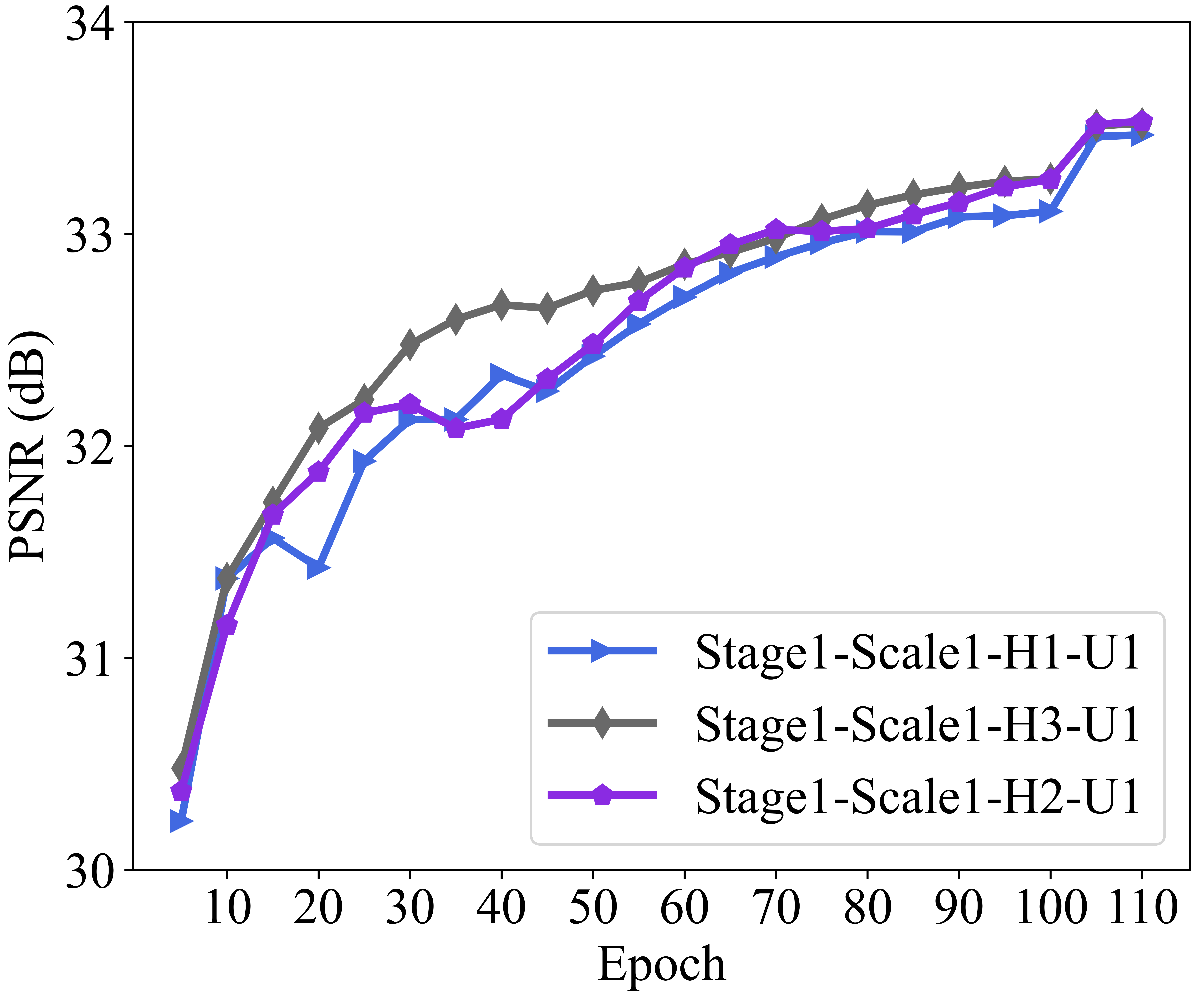
(a) Investigation of the RCABs number in $G_{k}(\cdot)$ and $\tilde{G}_{k}(\cdot)$

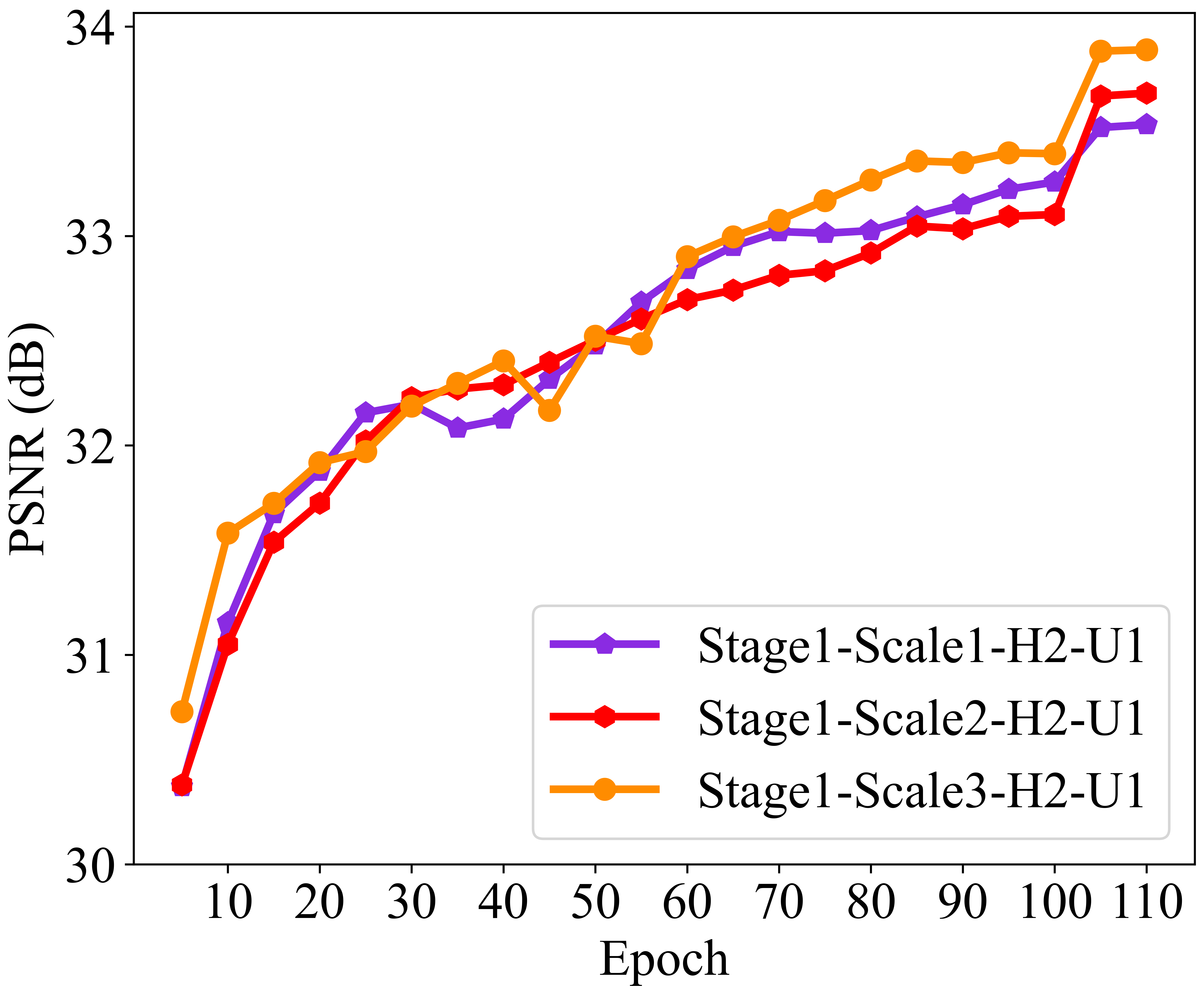
(b) Investigation of the scales number in $F_{k}(\cdot)$ and $\tilde{F}_{k}(\cdot)$

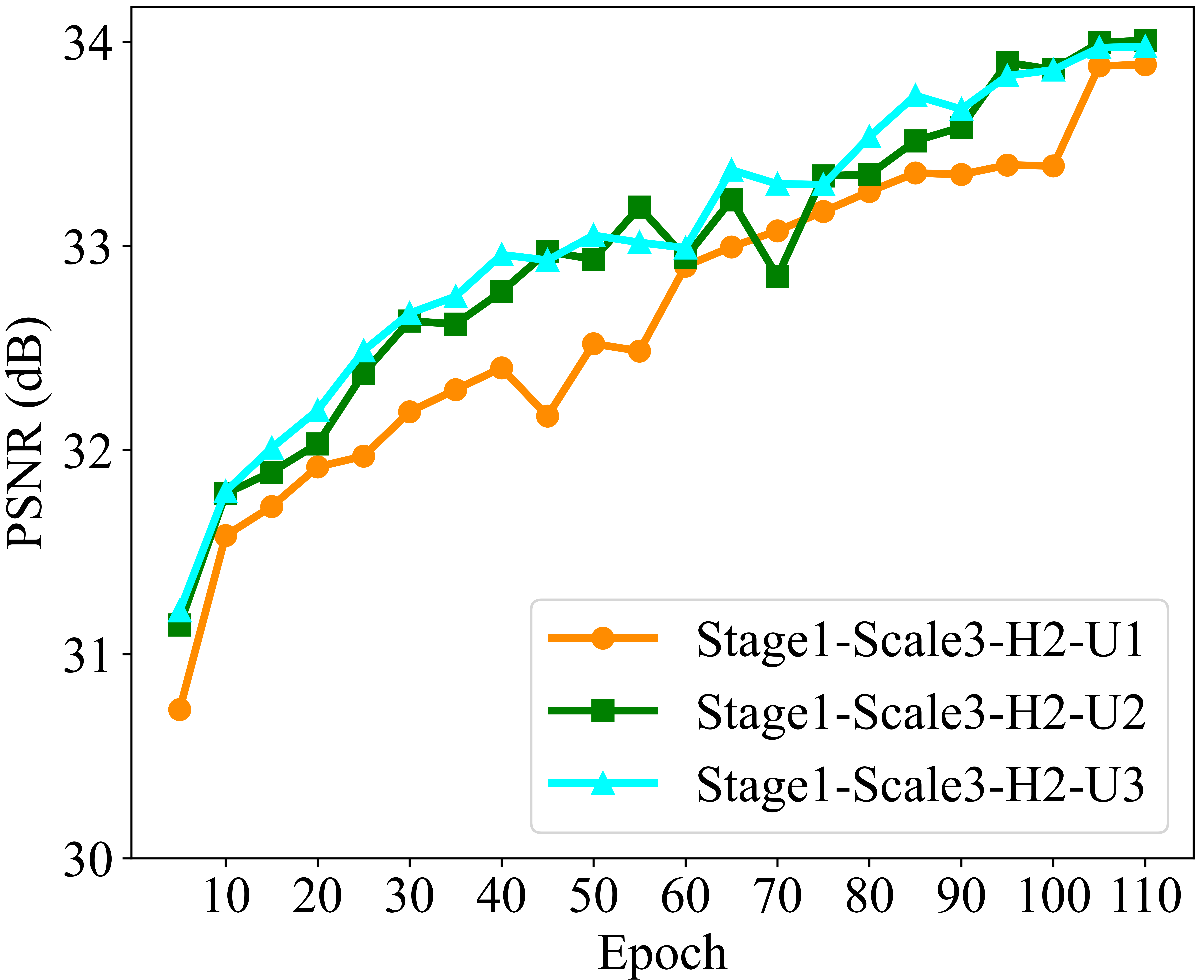
(c) Investigation of the RCABs number in Encoder-decoder

(d) Investigation of the stage number

Figure 2: Convergence analysis of MGSTNet for image deblurring with different structure.

III-A3 Parameter Setting

The AID dataset is utilized as the source of reference images during the training stage. We crop a $256\times 256$ patch from the sharp images and generate the corresponding degraded blur images with (1). The standard deviation $\sigma$ of the isotropic Gaussian blur kernel in (1) is randomly chosen from the range of [0.2, 4.0] and its size is set to $15\times 15$. The image pairs are then fed into the network for training.

During the testing stage, we apply the same random Gaussian blur to WHU-RS19 and use the synthesized WHU-RS19 as a test set to assess performance. To evaluate the image deblurring performance of WHU-RS19, we employ peak signal-to-noise ratio (PSNR), structural similarity (SSIM) [52] and the root mean square error (RMSE).

We randomly crop 1100 sharp image patches of size $256\times 256$ from the AIRS dataset for the experimental section. We then randomly select a Gaussian kernel standard deviation in the range of [1.0, 4.0] to generate sharp/blurred image pairs using (1). Of these, 1000 image pairs are used as the training dataset and 100 image pairs as the test dataset. To further examine the performance of each deblurring network in more complex degradation cases, Gaussian noise with a noise level of $10^{-3}$ is added to the blurred images of the AIRS dataset, which originally had a noise level close to $0$.

We train our network for 50 epochs for deblurring experiments on the AID and WHU-RS19 datasets, with the learning rate initially set to $10^{-4}$ and decreasing to $10^{-5}$ at 40 epochs. For the AIRS dataset, we train our network for 110 epochs, with an initial learning rate of $10^{-4}$ and decreasing to $10^{-5}$ at 100 epochs. The Adam optimizer [53] is used and all experiments are conducted using PyTorch.

TABLE I: Ablation study about the number of RCABs in the modules $G(\cdot)$ and $\tilde{G}(\cdot)$ by the proposed MGSTNet on the AIRS Dataset.

Method	MGSTNet
RCABs number in $G(\cdot)$ and $\tilde{G}(\cdot)$	1	2	3
PSNR	33.47	33.53	33.48
SSIM	0.8631	0.8642	0.8633
RMSE	6.4819	6.4481	6.4707

TABLE II: Ablation study about the blur kernel proximal mapping module by the proposed MGSTNet framework on the AIRS Dataset.

Method	MGSTNet
Kernel index	$s/||s||_{1}$	$h$
MNC	0.7036	0.9447
MSE	$7.9209\times 10^{-3}$	$2.0858\times 10^{-5}$
RMSE	$3.8036\times 10^{-2}$	$3.5029\times 10^{-3}$

TABLE III: Ablation study about the number of scales in the modules $F(\cdot)$ and $\tilde{F}(\cdot)$ by the proposed MGSTNet on the AIRS Dataset.

Method	MGSTNet
Scales number in $F(\cdot)$ and $\tilde{F}(\cdot)$	1	2	3
PSNR	33.53	33.66	33.88
SSIM	0.8642	0.8736	0.8832
RMSE	6.4481	6.2521	6.0307

TABLE IV: Ablation study about the number of RCABs in the modules $F(\cdot)$ and $\tilde{F}(\cdot)$ by the proposed MGSTNet on the AIRS Dataset.

Method	MGSTNet
RCABs number in $F(\cdot)$ and $\tilde{F}(\cdot)$	1	2	3
PSNR	33.88	33.99	33.97
SSIM	0.8832	0.8856	0.8856
RMSE	6.0307	5.9519	5.9787

TABLE V: Ablation study about the stage number of MGSTNet on the AIRS Dataset.

Method	MGSTNet
Stage number	1	2	3
PSNR	33.99	34.04	34.13
SSIM	0.8856	0.8878	0.8881
RMSE	5.9519	5.8842	5.8822

Figure 3: Visual comparison for different deblurring methods on AIRS datasets.

Figure 4: Visual comparison for different deblurring methods on AIRS datasets with small perturbation noise.

III-B Ablation Study and Architecture Discussion

Firstly, we conducted four groups of experiments on the AIRS dataset to determine the optimal configuration of the proposed MGSTNet for image deblurring. These experiments included the number of scales in $F(\cdot)$ and $\tilde{F}(\cdot)$, the number of RCABs in the $G(\cdot),\tilde{G}(\cdot)$, encoder and decoder, and the number of stages. To make it easier to assess reconstruction performance, all ablation studies were carried out with a stage number of $k=1$, except for the ablation study of the number of stages.

III-B1 Number of RCABs in $\bf{G_{k}(\cdot)}$ and $\bf{\tilde{G}_{k}(\cdot)}$

We illustrate the effect of depth on performance in blur kernel deep prior networks in Fig. 2(a) and Table I. It is evident that there is an improvement in image recovery when the number of RCABs increases from 1 to 2, but further increases do not lead to further gains. This demonstrates that learning the blur kernel deep prior can be achieved with a simpler network structure.

III-B2 The effective of KPMM

In order to illustrate the impact of the KPMM module on the blur kernel reconstruction performance, we evaluate the kernels using three metrics: MSE, RMSE, and maximum of normalized convolution (MNC)[54] in Table II. When the blur kernel goes through the gradient descent step, a preliminary blur kernel estimate $\bm{s}$ is obtained, but it is imprecise. After passing through the KPMM module, the loss of the blur kernel is significantly reduced, and the structural similarity with the Ground-truth kernel is greatly improved. Table II shows that the blur kernel depth prior can be learned through the KPMM module.

III-B3 Number of scales in $\bf{F_{k}(\cdot)}$ and $\bf{\tilde{F}_{k}(\cdot)}$

We demonstrate the effect of using multi-scale/single-scale thresholds in our network on the performance, as seen in Fig. 2(b) and Table III. It can be seen that the variant with multi-scale shrinkage thresholds yields better results across all three metrics compared to the single-scale thresholds. Without the multi-scale shrinkage thresholds, the PSNR will decrease by 0.35 dB. It is clear that the deblur performance of the proposed method with multi-scale prior is always better than that of the values with single-scale. This highlights the significance of incorporating multi-scale thresholding techniques in network design to improve image reconstruction quality.

III-B4 Number of RCABs in Encoder and Decoder

In this part, we investigate the advantages of having multiple RCABs in the Encoder and Decoder of the MGSTNet framework. As seen in Fig. 2(c) and Table IV, performance improves with the number of RCABs, which confirms the effectiveness of the image prior network design. To reconstruct a more accurate image geometric prior, we used two RCABs in our MGSTNet network.

III-B5 Number of stages

We investigate the correlation between the number of stages and the reconstruction performance by adjusting the stage number to $1$, $2$, and $3$. As seen in Fig. 2(d) and Table V, the performance improves with the number of stages, which confirms the effectiveness of the iterative network design. Therefore, we use three stages in our MGSTNet framework for the best reconstruction performance.

III-C Experiments on AIRS Dataset

To demonstrate the superiority of the proposed method, we compare it with several state-of-the-art methods on the synthetic AIRS dataset.

Figure 5: The PSNR box-plot of different deblurring methods on AIRS. ’(+)’ represents the deblurring performance experiment with noise.

TABLE VI: Performance comparisons of various deblurring methods on the AIRS datasets in terms of the interpretability, the estimation of the degradation kernel, the number of parameters, the average PSNR, the average SSIM, and the average RMSE. The semi-kernel estimation strategy in GKMNet denoted by utilizes a weighted combination of pre-defined Gaussian kernels for its kernel estimation, while NSM is a non-learning deblurring technique.

Method	Interpretability	Kernel estimated	Parameters	AIRS			AIRS(+)
				PSNR	SSIM	RMSE	PSNR	SSIM	RMSE
NSM [51]	✓	✓	–	28.24	0.6903	11.4925	28.23	0.6897	11.5033
DeblurGAN-v2 [25]	✗	✗	$60.90\text{M}$	28.53	0.7835	10.4392	27.17	0.6686	11.9058
GKMNet [30]	✓		$1.41\text{M}$	33.21	0.8667	6.5022	32.37	0.8681	6.9027
RDN [26]	✗	✗	$21.98\text{M}$	33.21	0.8782	6.4167	33.10	0.8708	6.5476
MIMO-UNet+ [29]	✗	✗	$16.11\text{M}$	33.19	0.8644	6.6661	33.13	0.8538	6.7964
SFNet [28]	✗	✗	$13.27\text{M}$	33.37	0.8769	6.4213	33.29	0.8748	6.5089
MGSTNet (Ours)	✓	✓	$15.23\text{M}$	34.13	0.8881	5.8822	33.81	0.8800	6.1090

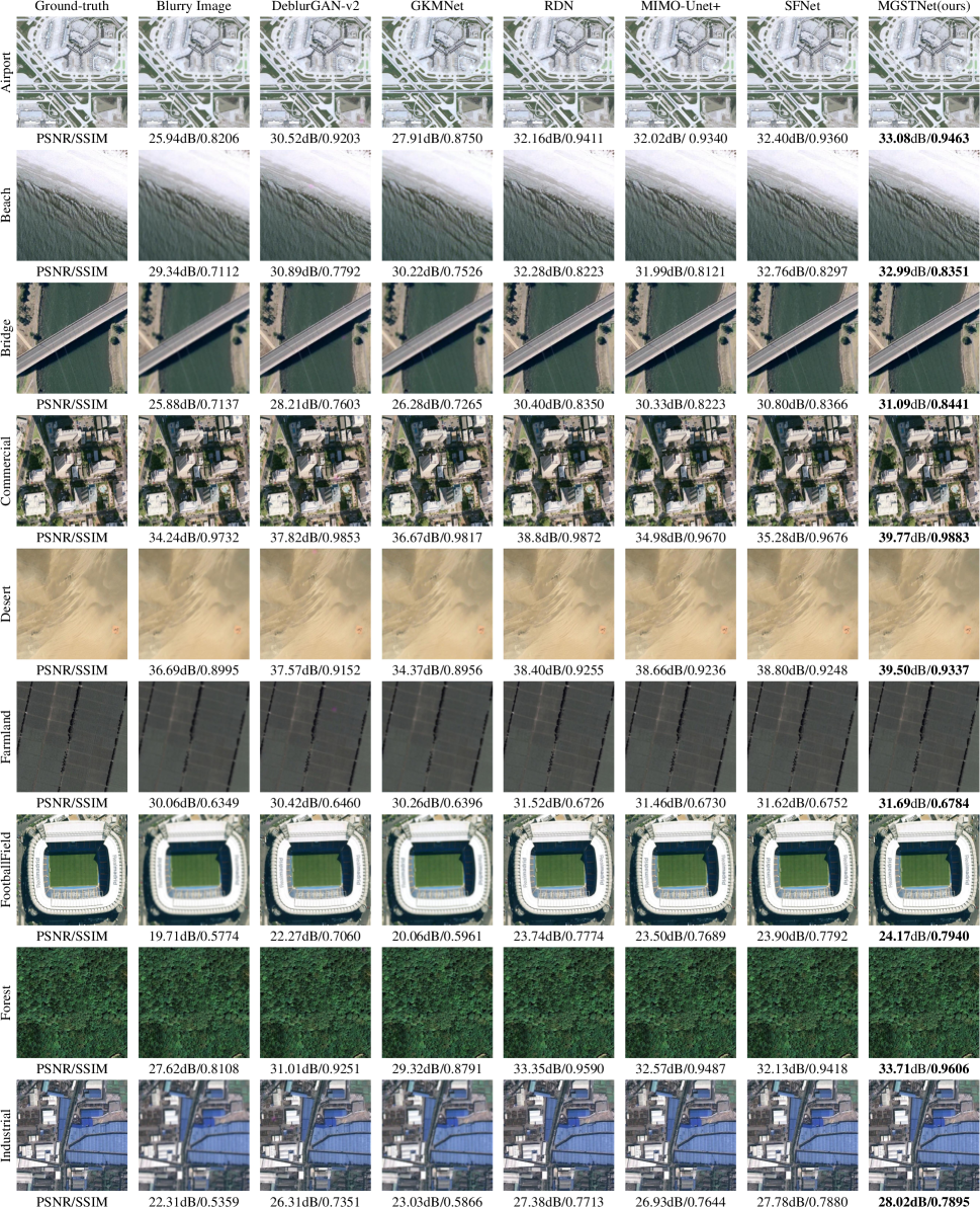
Figure 6: Visual comparison for different deblurring methods on WHU-RS19 datasets

TABLE VII: Comparison of different deblurring models on various scene classes of WHU-RS19 (PSNR ($dB$)/SSIM/RMSE). The best and second-best results are highlighted in Bold font and underlined ones, respectively.

WHU-RS19	RDN [26]	GKMNet [30]	DeblurGAN-v2 [25]	MIMO-UNet+ [29]	SFNet [28]	MGSTNet (Ours)
Airport	31.34/0.8719/8.327	27.36/0.7681/12.715	29.70/0.8364/9.858	30.13/0.8603/8.927	30.61/0.8706/8.3854	32.10/0.8824/7.712
Beach	40.96/0.9595/2.557	36.75/0.9477/3.853	38.65/0.9499/3.125	41.95/0.9641/2.290	41.16/0.9634/2.3939	43.69/0.9733/1.866
Bridge	35.33/0.9181/5.067	31.53/0.8709/7.663	32.27/0.8921/6.645	34.26/0.9082/5.462	34.74/0.9115/5.1385	36.13/0.9222/4.738
Commercial	29.27/0.8586/10.606	25.43/0.7225/16.449	27.48/0.8196/12.525	27.86/0.8433/11.592	28.32/0.8559/10.8720	29.68/0.8655/10.155
Desert	40.14/0.9289/2.791	35.18/0.9013/4.565	38.31/0.9166/3.302	38.94/0.9188/3.064	39.03/0.9191/3.0267	40.71/0.9309/2.661
Farmland	37.67/0.8903/3.879	34.86/0.8520/5.106	35.98/0.8726/4.451	36.41/0.8804/4.227	36.83/0.8872/4.0008	38.46/0.8987/3.577
FootballField	33.70/0.9033/6.694	29.36/0.8217/10.688	31.61/0.8774/8.097	31.99/0.8918/7.362	32.34/0.8977/6.9886	34.64/0.9119/6.123
Forest	30.62/0.7967/8.490	27.90/0.6452/11.421	28.67/0.7451/10.292	29.64/0.7909/9.128	29.89/0.7989/8.7654	30.93/0.8109/8.242
Industrial	29.51/0.8545/9.845	25.80/0.7199/15.233	28.26/0.8183/11.365	28.84/0.8441/10.360	29.42/0.8573/9.6288	30.41/0.8675/9.051
Meadow	38.46/0.8949/3.453	35.62/0.8536/4.585	36.11/0.8684/4.283	37.33/0.8848/3.774	37.39/0.8831/3.7476	38.55/0.8890/4.054
Mountain	27.64/0.7764/12.220	25.08/0.6298/16.094	25.08/0.6298/16.094	26.49/0.7639/13.250	26.81/0.7747/12.6483	27.74/0.7856/11.960
Park	30.16/0.8263/9.129	27.16/0.7123/12.760	28.94/0.7881/10.438	29.37/0.8124/9.742	29.81/0.8230/9.2036	30.71/0.8310/8.789
Parking	29.37/0.8837/10.035	25.32/0.7585/16.172	28.22/0.8551/11.358	28.84/0.8757/10.387	29.76/0.8894/9.3269	30.51/0.8980/8.937
Pond	34.00/0.8940/6.153	30.88/0.8308/8.630	31.77/0.8663/7.511	32.79/0.8852/6.633	33.20/0.8891/6.2910	34.59/0.8994/5.850
Port	30.60/0.8927/8.983	26.66/0.8010/14.186	28.12/0.8586/11.225	29.33/0.8765/10.062	29.95/0.8861/9.1669	30.95/0.8966/8.630
RailwayStation	28.67/0.8086/11.108	25.53/0.6755/15.625	27.41/0.7707/12.514	27.60/0.7979/11.862	28.04/0.8066/11.2312	28.89/0.8105/10.778
Residential	28.85/0.8797/10.263	24.38/0.7425/17.302	27.26/0.8415/12.360	28.13/0.8674/10.970	28.78/0.8797/10.1370	29.50/0.8898/9.599
River	32.87/0.8648/7.115	30.39/0.7852/9.458	31.04/0.8320/8.451	31.42/0.8520/7.854	31.68/0.8575/7.5355	33.52/0.8714/6.791
Viaduct	30.24/0.8761/9.271	26.32/0.7491/14.714	28.55/0.8389/11.122	29.14/0.8653/9.972	29.44/0.8723/9.5311	31.02/0.8855/8.669
Average	32.60/0.8727/7.679	29.03/0.7783/11.432	30.75/0.8404/9.107	31.59/0.8623/8.257	31.95/0.8697/7.7905	33.29/0.8800/7.276

Table VI shows that DeblurGANv2, RDN, MIMO-UNet+, and SFNet are black box models, which lack transparency and interpretability. On the other hand, NSM and MGSTNet are based on model-driven theory to create blur kernel estimation learning modules. GKMNet, meanwhile, uses a weighted combination of pre-defined Gaussian kernels for its kernel estimation. All six of the compared techniques, with the exception of NSM, are based on deep learning, which is more powerful than traditional image deblurring approaches. MGSTNet has more parameters than GKMNet due to the image/kernel prior features needed for image deblurring. Despite this, MGSTNet still has a reasonable number of parameters and achieves the best image blind deblurring performance among all the compared approaches.

Table VI presents a quantitative comparison of the deblurring effects for a given experimental setup, with AIRS(+) indicating performance with small perturbation noise. The quality of the original image is degraded when noise is added, making it difficult to extract feature information. Therefore, image deblurring methods need to have strong detail reconstruction capability. Our method outperforms other state-of-the-art methods in both remote sensing image deblurring tasks, with an average 0.76 dB improvement on the AIRS dataset. The performance of the various methods decreases as a result of the addition of noise, with the NSM remaining relatively stable. GKMNet, RDN, and MIMO-UNet+ all show different levels of performance degradation. Nevertheless, our method still has superior performance compared to other deblurring methods.

The box-plot is a statistical representation of the discrete degree of a data group, which can be used to evaluate the stability of the deblurring effect. It consists of five lines that represent the minimum, first quartile (Q1), median, third quartile (Q3), and maximum values of the data, respectively. The Interquartile Range (IQR) is the difference between the third and first quartiles, $IQR=Q3-Q1$, and is used to measure the discrete degree of the data. Outliers are defined as data points that are more than 1.5 IQR away from either the Q1 or Q3.

As illustrated in Fig. 5, all deblurring methods except MIMO-UNet+ have outliers (diamonds on the left side of Fig. 5). This is because MIMO-UNet+ has an excessively high interquartile range (IQR) and its overall performance is unstable. In terms of outliers, the lower performance bound of MGSTNet is higher than that of the other deblurring methods. In experiments without noise, our method achieved the highest Q1 value (30.9293), the median value (33.4711), and the Q3 value (37.9882). When it comes to deblurring with noise, our approach had the highest Q1 (30.5682), median (33.6052), and second highest Q3 value (37.7561) after MIMO-UNet+ (37.7601). Therefore, MGSTNet performs better than the other methods in deblurring tasks.

Figs. 3 and 4 show deblurring reconstructions from various methods. Our approach is successful in eliminating blur degradation, resulting in a sharper image and one that is closer to the ground truth in visual perception than other comparison methods. In contrast, the deblurred outputs of MIMO-UNet+, GKMNet, and RDN have visible artifacts. The comparison in Figs. 3 and 4 demonstrates that our MGSTNet can effectively recover detailed information from the deblurred image, making its performance superior to that of the other compared methods. In addition, MGSTNet also performs well in dealing with the deblurring problem with noise.

III-D Experiments on AID, WHU-RS19 Dataset

To demonstrate the generalizability of our model, we also perform image deblurring on AID and WUH-19 with lower spatial resolution. The results of the WHU-RS19 dataset are shown in Table VII. Our approach achieved the best reconstruction performance for the deblurring of 19 remote sensing images, with an average improvement of 0.69 dB. Generally, the deblurring performance was better for images with simpler structures, such as Beach and Desert, and slightly worse for images with more intricate structures, such as Commercial, Mountain, RailwayStation, and Residential. Other images with complex structures had slightly lower deblurring performance.

Fig. 6 illustrates a visual comparison of the deblurring results of various methods on the WHU-RS19 dataset. While other approaches have some success in restoring the blurred input image, they are unable to fully recover local textures and structures in detail. GKMNet, which does not have any prior modules, performs worse than the pure network DeblurGAN-v2. On the other hand, MIMO-Unet+ and RDN, which have a more complex network structure to extract richer features than DeblurGAN-v2, achieve better deblurring performance. In contrast, our method can recover the details and edges of the image more effectively, resulting in the sharpest and most accurate remote sensing images.

IV Conclusion

This paper introduces a novel image blind deblurring network architecture based on bilayer alternating iterations of linear reconstruction and shrinkage thresholds to restore remote sensing images, which alternately evolves the blurring kernels and images. The theoretical basis of the network design is also provided. Additionally, a multi-scale encoder-decoder network is proposed to composite feature spaces to learn image feature representations on different scales. This network is used to learn nonlinear spatial transformations to extract abstract feature information for multi-scale representations. To improve the assessment of the blur kernel, a blur kernel proximal mapping module is proposed. Furthermore, a multi-scale shrinkage thresholding strategy is used to ensure a rich representation of the feature space. The results of state-of-the-art qualitative and quantitative evaluations on a synthetic remote sensing deblurred dataset demonstrate the effectiveness of our method. Moreover, the robustness of our approach to recover good images under blur and small noise is also demonstrated.

References

- [1] G. Cheng, P. Zhou, and J. Han, “Learning rotation-invariant convolutional neural networks for object detection in vhr optical remote sensing images,” IEEE Transactions on Geoscience and Remote Sensing, vol. 54, no. 12, pp. 7405–7415, 2016.
- [2] Z. Deng, H. Sun, S. Zhou, J. Zhao, L. Lei, and H. Zou, “Multi-scale object detection in remote sensing imagery with convolutional neural networks,” ISPRS journal of photogrammetry and remote sensing, vol. 145, pp. 3–22, 2018.
- [3] D. Yu and S. Ji, “A new spatial-oriented object detection framework for remote sensing images,” IEEE Transactions on Geoscience and Remote Sensing, vol. 60, pp. 1–16, 2021.
- [4] L. Wang, R. Li, C. Zhang, S. Fang, C. Duan, X. Meng, and P. M. Atkinson, “Unetformer: A unet-like transformer for efficient semantic segmentation of remote sensing urban scene imagery,” ISPRS Journal of Photogrammetry and Remote Sensing, vol. 190, pp. 196–214, 2022.
- [5] C. Chen and L. Fan, “Scene segmentation of remotely sensed images with data augmentation using u-net++,” in 2021 International Conference on Computer Engineering and Artificial Intelligence (ICCEAI). IEEE, 2021, pp. 201–205.
- [6] X. Wang, L. Cavigelli, M. Eggimann, M. Magno, and L. Benini, “Hr-sar-net: A deep neural network for urban scene segmentation from high-resolution sar data,” in 2020 IEEE Sensors Applications Symposium (SAS). IEEE, 2020, pp. 1–6.
- [7] X. Wang, X. Wang, R. Song, X. Zhao, and K. Zhao, “Mct-net: Multi-hierarchical cross transformer for hyperspectral and multispectral image fusion,” Knowledge-Based Systems, vol. 264, p. 110362, 2023.
- [8] Q. Xie, M. Zhou, Q. Zhao, Z. Xu, and D. Meng, “Mhf-net: An interpretable deep network for multispectral and hyperspectral image fusion,” IEEE Transactions on Pattern Analysis and Machine Intelligence, vol. 44, no. 3, pp. 1457–1473, 2020.
- [9] H. Shen, M. Jiang, J. Li, C. Zhou, Q. Yuan, and L. Zhang, “Coupling model-and data-driven methods for remote sensing image restoration and fusion: Improving physical interpretability,” IEEE Geoscience and Remote Sensing Magazine, vol. 10, no. 2, pp. 231–249, 2022.
- [10] A. Buades, B. Coll, and J.-M. Morel, “A non-local algorithm for image denoising,” in 2005 IEEE computer society conference on computer vision and pattern recognition (CVPR’05), vol. 2. Ieee, 2005, pp. 60–65.
- [11] K. Dabov, A. Foi, V. Katkovnik, and K. Egiazarian, “Image denoising by sparse 3-d transform-domain collaborative filtering,” IEEE Transactions on image processing, vol. 16, no. 8, pp. 2080–2095, 2007.
- [12] T. F. Chan and C.-K. Wong, “Total variation blind deconvolution,” IEEE transactions on Image Processing, vol. 7, no. 3, pp. 370–375, 1998.
- [13] Q. Shan, J. Jia, and A. Agarwala, “High-quality motion deblurring from a single image,” Acm transactions on graphics (tog), vol. 27, no. 3, pp. 1–10, 2008.
- [14] L. Xu, S. Zheng, and J. Jia, “Unnatural l0 sparse representation for natural image deblurring,” in Proceedings of the IEEE conference on computer vision and pattern recognition, 2013, pp. 1107–1114.
- [15] Y. Luo, Y. Xu, and H. Ji, “Removing rain from a single image via discriminative sparse coding,” in Proceedings of the IEEE international conference on computer vision, 2015, pp. 3397–3405.
- [16] M. Aharon, M. Elad, and A. Bruckstein, “K-svd: An algorithm for designing overcomplete dictionaries for sparse representation,” IEEE Transactions on signal processing, vol. 54, no. 11, pp. 4311–4322, 2006.
- [17] J. Mairal, M. Elad, and G. Sapiro, “Sparse representation for color image restoration,” IEEE Transactions on image processing, vol. 17, no. 1, pp. 53–69, 2007.
- [18] D. Krishnan and R. Fergus, “Fast image deconvolution using hyper-laplacian priors,” Advances in neural information processing systems, vol. 22, 2009.
- [19] J. Pan, D. Sun, H. Pfister, and M.-H. Yang, “Blind image deblurring using dark channel prior,” in Proceedings of the IEEE conference on computer vision and pattern recognition, 2016, pp. 1628–1636.
- [20] X. Mao, Y. Liu, W. Shen, Q. Li, and Y. Wang, “Deep residual fourier transformation for single image deblurring,” arXiv preprint arXiv:2111.11745, 2021.
- [21] D. Ren, K. Zhang, Q. Wang, Q. Hu, and W. Zuo, “Neural blind deconvolution using deep priors,” in Proceedings of the IEEE/CVF Conference on Computer Vision and Pattern Recognition, 2020, pp. 3341–3350.
- [22] J. Li, Y. Nan, and H. Ji, “Un-supervised learning for blind image deconvolution via monte-carlo sampling,” Inverse Problems, vol. 38, no. 3, p. 035012, 2022.
- [23] S. Nah, T. H. Kim, and K. M. Lee, “Deep multi-scale convolutional neural network for dynamic scene deblurring,” in The IEEE Conference on Computer Vision and Pattern Recognition (CVPR), July 2017.
- [24] O. Kupyn, V. Budzan, M. Mykhailych, D. Mishkin, and J. Matas, “Deblurgan: Blind motion deblurring using conditional adversarial networks,” in Proceedings of the IEEE conference on computer vision and pattern recognition, 2018, pp. 8183–8192.
- [25] O. Kupyn, T. Martyniuk, J. Wu, and Z. Wang, “Deblurgan-v2: Deblurring (orders-of-magnitude) faster and better,” in Proceedings of the IEEE/CVF international conference on computer vision, 2019, pp. 8878–8887.
- [26] Y. Zhang, Y. Tian, Y. Kong, B. Zhong, and Y. Fu, “Residual dense network for image restoration,” IEEE Transactions on Pattern Analysis and Machine Intelligence, vol. 43, no. 7, pp. 2480–2495, 2020.
- [27] X. Mao, Y. Liu, F. Liu, Q. Li, W. Shen, and Y. Wang, “Intriguing findings of frequency selection for image deblurring,” arXiv e-prints, pp. arXiv–2111, 2021.
- [28] Y. Cui, Y. Tao, Z. Bing, W. Ren, X. Gao, X. Cao, K. Huang, and A. Knoll, “Selective frequency network for image restoration,” in The Eleventh International Conference on Learning Representations, 2022.
- [29] S.-J. Cho, S.-W. Ji, J.-P. Hong, S.-W. Jung, and S.-J. Ko, “Rethinking coarse-to-fine approach in single image deblurring,” in Proceedings of the IEEE/CVF international conference on computer vision, 2021, pp. 4641–4650.
- [30] Y. Quan, Z. Wu, and H. Ji, “Gaussian kernel mixture network for single image defocus deblurring,” Advances in Neural Information Processing Systems, vol. 34, pp. 20 812–20 824, 2021.
- [31] S. Xu, J. Zhang, Z. Zhao, K. Sun, J. Liu, and C. Zhang, “Deep gradient projection networks for pan-sharpening,” in Proceedings of the IEEE/CVF Conference on Computer Vision and Pattern Recognition, 2021, pp. 1366–1375.
- [32] Y. Li, M. Tofighi, J. Geng, V. Monga, and Y. C. Eldar, “Efficient and interpretable deep blind image deblurring via algorithm unrolling,” IEEE Transactions on Computational Imaging, vol. 6, pp. 666–681, 2020.
- [33] J. Zhang and B. Ghanem, “Ista-net: Interpretable optimization-inspired deep network for image compressive sensing,” in Proceedings of the IEEE conference on computer vision and pattern recognition, 2018, pp. 1828–1837.
- [34] D. You, J. Xie, and J. Zhang, “Ista-net++: flexible deep unfolding network for compressive sensing,” in 2021 IEEE International Conference on Multimedia and Expo (ICME). IEEE, 2021, pp. 1–6.
- [35] X. Fan, Y. Yang, and J. Zhang, “Deep geometric distillation network for compressive sensing MRI,” in 2021 IEEE EMBS International Conference on Biomedical and Health Informatics (BHI), jul 2021.
- [36] H. Zhu, S. Shu, and J. Zhang, “Fas-unet: A novel fas-driven unet to learn variational image segmentation,” Mathematics, vol. 10, no. 21, p. 4055, Nov 2022.
- [37] X. Fan, Y. Yang, K. Chen, J. Zhang, and K. Dong, “An interpretable MRI reconstruction network with two-grid-cycle correction and geometric prior distillation,” Biomedical Signal Processing and Control, vol. 84, p. 104821, Jul 2023.
- [38] A. Liu, X. Fan, Y. Yang, and J. Zhang, “PRISTA-Net: Deep Iterative Shrinkage Thresholding Network for Coded Diffraction Patterns Phase Retrieval,” arXiv e-prints, p. arXiv:2309.04171, Sept 2023.
- [39] X. Fan, Y. Yang, K. Chen, Y. Feng, and J. Zhang, “Nest-DGIL: Nesterov-optimized Deep Geometric Incremental Learning for CS Image Reconstruction,” arXiv e-prints, p. arXiv:2308.03807, Aug. 2023.
- [40] Z. Cui, C. Liu, X. Fan, C. Cao, J. Cheng, Q. Zhu, Y. Liu, S. Jia, Y. Zhou, H. Wang, Y. Zhu, J. Zhang, Q. Liu, and D. Liang, “Physics-informed deepmri: Bridging the gap from heat diffusion to k-space interpolation,” CoRR, vol. abs/2308.15918, 2023. [Online]. Available: https://doi.org/10.48550/arXiv.2308.15918
- [41] X. Kang, J. Li, P. Duan, F. Ma, and S. Li, “Multilayer degradation representation-guided blind super-resolution for remote sensing images,” IEEE Transactions on Geoscience and Remote Sensing, vol. 60, pp. 1–12, 2022.
- [42] C. Mou, Q. Wang, and J. Zhang, “Deep generalized unfolding networks for image restoration,” in Proceedings of the IEEE/CVF Conference on Computer Vision and Pattern Recognition, 2022, pp. 17 399–17 410.
- [43] A. Levin, R. Fergus, F. Durand, and W. T. Freeman, “Image and depth from a conventional camera with a coded aperture,” ACM transactions on graphics (TOG), vol. 26, no. 3, pp. 70–es, 2007.
- [44] Y. Zhang, K. Li, K. Li, L. Wang, B. Zhong, and Y. Fu, “Image super-resolution using very deep residual channel attention networks,” in Proceedings of the European conference on computer vision (ECCV), 2018, pp. 286–301.
- [45] W. Zuo, D. Meng, L. Zhang, X. Feng, and D. Zhang, “A generalized iterated shrinkage algorithm for non-convex sparse coding,” in Proceedings of the IEEE international conference on computer vision, 2013, pp. 217–224.
- [46] F.-J. Tsai, Y.-T. Peng, C.-C. Tsai, Y.-Y. Lin, and C.-W. Lin, “Banet: A blur-aware attention network for dynamic scene deblurring,” IEEE Transactions on Image Processing, vol. 31, pp. 6789–6799, 2022.
- [47] S. W. Zamir, A. Arora, S. Khan, M. Hayat, F. S. Khan, M.-H. Yang, and L. Shao, “Multi-stage progressive image restoration,” in Proceedings of the IEEE/CVF conference on computer vision and pattern recognition, 2021, pp. 14 821–14 831.
- [48] Q. Chen, L. Wang, Y. Wu, G. Wu, Z. Guo, and S. L. Waslander, “Temporary removal: Aerial imagery for roof segmentation: A large-scale dataset towards automatic mapping of buildings,” ISPRS journal of photogrammetry and remote sensing, vol. 147, pp. 42–55, 2019.
- [49] G.-S. Xia, J. Hu, F. Hu, B. Shi, X. Bai, Y. Zhong, L. Zhang, and X. Lu, “Aid: A benchmark data set for performance evaluation of aerial scene classification,” IEEE Transactions on Geoscience and Remote Sensing, vol. 55, no. 7, pp. 3965–3981, 2017.
- [50] D. Dai and W. Yang, “Satellite image classification via two-layer sparse coding with biased image representation,” IEEE Geoscience and remote sensing letters, vol. 8, no. 1, pp. 173–176, 2010.
- [51] D. Krishnan, T. Tay, and R. Fergus, “Blind deconvolution using a normalized sparsity measure,” in CVPR 2011. IEEE, 2011, pp. 233–240.
- [52] Z. Wang, A. C. Bovik, H. R. Sheikh, and E. P. Simoncelli, “Image quality assessment: from error visibility to structural similarity,” IEEE transactions on image processing, vol. 13, no. 4, pp. 600–612, 2004.
- [53] D. P. Kingma and J. Ba, “Adam: A method for stochastic optimization,” arXiv preprint arXiv:1412.6980, 2014.
- [54] Z. Hu and M.-H. Yang, “Good regions to deblur,” in Computer Vision–ECCV 2012: 12th European Conference on Computer Vision, Florence, Italy, October 7-13, 2012, Proceedings, Part V 12. Springer, 2012, pp. 59–72.