MuLaN: a MultiLayer Networks Alignment Algorithm

Abstract

A Multilayer Network (MN) is a system consisting of several topological levels (i.e., layers) representing the interactions between the system’s objects and the related interdependency. Therefore, it may be represented as a set of layers that can be assimilated to a set of networks of its own objects, by means inter-layer edges (or inter-edges) linking the nodes of different layers; for instance, a biological MN may allow modeling of inter and intra interactions among diseases, genes, and drugs, only using its own structure. The analysis of MNs may reveal hidden knowledge, as demonstrated by several algorithms for the analysis. Recently, there is a growing interest in comparing two MNs by revealing local regions of similarity, as a counterpart of Network Alignment algorithms (NA) for simple networks. However, classical algorithms for NA such as Local NA (LNA) cannot be applied on multilayer networks, since they are not able to deal with inter-layer edges. Therefore, there is the need for the introduction of novel algorithms. In this paper, we present MuLaN, an algorithm for the local alignment of multilayer networks. We first show as proof of concept the performances of MuLaN on a set of synthetic multilayer networks. Then, we used as a case study a real multilayer network in the biomedical domain. Our results show that MuLaN is able to build high-quality alignments and can extract knowledge about the aligned multilayer networks.
MuLaN is available at https://github.com/pietrocinaglia/mulan.

1 Introduction

Networks are largely used to represent entities and their association in many fields [1, 2, 3]. For instance, in computational biology and bioinformatics, networks are used to model the set of association among genes, proteins and other macromolecules [4, 5, 6]. More recently, it has been shown that a single level of representation, i.e., considering only genes, or only proteins, may result in a loss of information, so the need for introduction of other models arise. Such models are based on a multilevel (or multilayered) view of a system. As an example, in the biological scenario, each level may correspond to a different view, e.g. genes, proteins, and diseases. In such a view, each layer is composed by a set of homogeneous nodes linked by edges (i.e., intra-layer edges). Associations between two different layers are modelled by cross layer edges (i.e., inter-layer edges) [7, 8]. Figure 1 represents a non-exhaustive example of a simple multilayer network having three layers. Each layer is a different network. Figure 2 depicts an example of a biological multilayer network representing the interplay between diseases and drugs.

Figure 1: A non-exhaustive example of multilayer network. The figure represents a network in a multilayer prospective. The same entities are modeled as nodes of a same layer, and their interactions consists of intra-edges. Otherwise, the nodes of different layers are connected by inter-edges.

Figure 2: The figure shows a toy example of a biological multilayer network, representing disease-drug associations. The nodes are the diseases and the drugs, both discriminated by belonging to the respective layer. The intra-edges represent the drug-drug and the disease-disease associations, while the inter-edges the disease-drug associations. For instance, these may be analyzed to investigate the mechanisms underlying the interaction between diseases and drugs, or for computational drug repositoring.

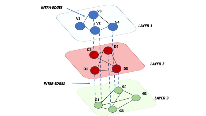
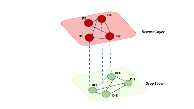
Formally, a multilayer graph may be described as a tuple $G_{M}=(V_{M},E_{M},V,L)$, where $V_{M}$ and $E_{M}$ are a set of nodes and edges, respectively, and $L$ is a set of layers. Thus, given $L=\{L_{1},L_{2},...,L_{k}\}$, with $k$ the number of layers in the multilayer graph, the nodes as pairs $V_{M}\subseteq VxL_{1}x...L_{k}$, the edges $E_{M}\subseteq V_{M}xV_{M}$ connect the pairs $(v,l)$, $(v^{\prime},l^{\prime})$. In a multilayer graph, an edge is defined intra-layer in case of $l$ is equal to $l^{\prime}$ or inter-layer, in case of $l$ and $l^{\prime}$ are different [9].

In general, the analysis of networks is rarely simple. Common challenges that can be generalized for all types of networks concern i) the modelling of the network, i.e., what it represents and ii) the analysis of the network, i.e., the metrics grabbing the biological phenomenon of interest. These aspects are at least as important for multilayer networks, given their added complexity. Furthermore, there are additional observations that are different to multilayer networks with respect to classical networks. For instance, an analysis should take into account the difference among layers. In particular, since the strength of multilayer network analysis consists of the capability to include information on different type of relationship, it would be necessary to consider which layers should be included in the analysis, and the interpretation of intra-layer and inter-layer edges values, since they discriminate against the different relationships.

The analysis of networks enables to find interesting regions of similarity between them [10, 11]. For simple networks, this task is accomplished by means of Network Alignment (NA) algorithms. Unfortunately, as also evidenced in [12, 13, 14], existing alignment algorithms are unable to process multilayer networks. Therefore, the need for defining a novel multilayer network algorithm arises. We focused in particular on evidencing relatively small regions of similarity among the multilayer networks, so we extended the Local Network Algorithm approaches. In a previous work [14], we presented MultiLoAl for the local alignment of multilayer networks. Despite the effectiveness of the approach, it presented some limitations related to the scalability on large datasets and on the topological structure of the region of the similarity.

Therefore, we extended our methodology to admit further topological structures of the found regions as well as better to obtain performances in terms of quality and running time. Such a methodology has been implemented in a novel tool, namely MuLaN (from MultiLAyer Network Alignment Algorithm). It consists of a novel approach for the building of alignment graph who achieves better performances, and it is integrated with a set of community discover algorithms enabling to discover regions of similarity with different topological structures.

Summarizing, MuLaN allows you to mainly benefit from the following advantages, compared to MultiLoAl: (i) a reduction of running time for building the alignment graph, and (ii) a deeper experimentation on a larger dataset.

MuLaN is based on the workflow depicted in Figure 3.

Figure 3: Workflow of the proposed algorithm.

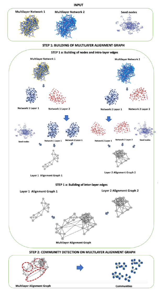
It receives as input two multilayer networks ($M_{1}$ and $M_{2}$) having the same number of layers $n$. Without loss of generality, we suppose the existence of a bijective correspondence among layers of the networks, so the layer $k$ in 1-$n$ of $M_{1}$ corresponds to the layer $k$ of $M_{2}$. MuLaN also receives a multiset of seed nodes representing the similarity between the node of the graph of the same layer $k$ of the two networks. Starting from $M_{1}$ and $M_{2}$ and multiset of seed nodes, at first, MuLaN analyzes each pair of $k$ layers in $M_{1}$ and $M_{2}$ independently. Then, it builds $n$ alignment graphs. After building each alignment graph for each $k$ layer separately, MuLaN analyzes $M_{1}$ and $M_{2}$ to add inter-layer edges among $n$ alignment graphs. Thus, the algorithms build $n-1$ alignment graphs, that we call multilayer alignment graphs. Finally, MuLaN applies a community detection algorithm suitable for multilayer networks on the final multilayer alignment graph to detect communities representing local regions of similarity, i.e. a single region of the local alignment. The current version of MuLaN offer three different community discover algorithms: Louvain [15], Infomap [16] and Greedy [17].

We implemented three versions of MuLaN by varying the community detection method. The default version applies Louvain [15] to mine community from the multilayer alignment graph, whereas, the other two versions use Infomap [16] and Greedy [17] as community detection algorithms, respectively [18].

The rest of this paper is organized as follows. Section 2 discusses the background on multilayer networks and multilayer community detection, Section 3 presents the MuLaN Algorithm, and Section 4 presents and discusses the results. Finally, Section 5 concludes the paper.

2 Related Work

We report here some existing state-of-the-art approaches for the analysis of MNs. We separate the algorithms that analyze a single network from those comparing two networks [19].

2.1 Network Alignment Algorithms

The problem of graph alignment consists of finding a mapping between nodes of two or more graphs to maximize an associated cost function. Formally, let $G_{1}=\{V_{1},E_{1}\}$ and $G_{2}=\{V_{2},E_{2}\}$ two graphs, where $V_{1,2}$ are sets of nodes and $E_{1,2}$ are sets of edges, the graph alignment problem consists of finding a function (or a mapping) $f:V_{1}\rightarrow V_{2}$ such that the similarity between mapped entities is maximized. Among the others, algorithms may be categorised in global network alignment (GNA) algorithms (i.e. algorithms that aim to find a single mapping among all the nodes of the networks), or local network alignment (LNA) algorithms (i.e. algorithms aiming at finding multiple small regions of similarity among networks).

We here report some LNA algorithms, since MuLaN search for multiple regions of similarity in multilayer networks.

An example of LNA algorithm is AlignNemo [20] that enables the discovery of subnetworks of proteins related to biological function and topology. AlignMCL [21] extends AlignNemo [20], by providing a formal definition of the alignment graph, which is clustered by using the Markov cluster algorithm MCL [22].

Also, GLAlign (Global Local Aligner) [23] combines the topology information from global alignment with biological information (e.g. homology relationships) to build local network alignment. NetworkBLAST [24] aims to find small dense regions in protein-protein interaction networks. Such subgraphs represent protein complexes, i.e. groups of proteins performing a similar function or involved in the same biological process. NetAligner [25] presents a strategy to identify evolutionarily conserved interactions on the basis of the consideration that interacting proteins evolve at rates significantly closer than expected by chance. Furthermore, L-HetNetAligner [12] extends the local alignment to the heterogeneous networks. Finally, some recent papers focused on the alignment of dynamic or dual networks [26, 27, 5]. However, these network alignment algorithms do not perform very well for multilayer networks [7, 28].

2.2 Community Detection in Multilayer Networks

Community detection algorithms aim to identify groups of nodes closely connected with respect to the average of the network, starting from the assumption that nodes in the same community have a similar role [29, 30, 31]. In detail, a community is defined as groups of nodes that are more densely connected than the rest of the network; they represent significant characteristics for understanding the functionalities and organizations of complex systems modeled as a network.

In multilayer networks, the communities represent groups of well-connected nodes considering whole layers, community detection methods should consider the diversity between the layers[18].

To handle these issues, many community detection algorithms for multilayer networks have been recently developed.

The Louvain algorithm, initially developed for simple networks, has been extended to handle multilayer networks [15]. The algorithms are based on an ad hoc defined notion of modularity for multilayer network, which is based on the definition of community as a set of nodes and edges belonging to multiple layers. Therefore, the algorithm applies an iterative greedy approach to build communities.

Infomap [16, 32] discovers communities in multilayer networks by running random walks, admitting also interlayer edges. Infomap can be used to find both overlapping and non-overlapping communities.

Greedy [17] algorithm is a simple and fast community detection method that works by greedily optimizing a quality function known as modularity. The algorithm starts with each node in its own community and iteratively merges communities that increase the modularity at the most.

ABACUS [33] algorithm enables to extract multidimensional communities by mining frequent closed item sets on one-dimensional community memberships. Initially, it extracts one-dimensional communities, looking at each dimension. Then, ABACUS assigns a label to nodes that consists in a list of pair tags (e.g., dimension and community). After that, ABACUS uses a frequent closed item set mining algorithm by treating each pair of tags as an item. At the end, the multidimensional communities described by the item sets consist of frequent closed item sets.

Multi-Layer Clique Percolation [34] method applies the classical clique percolation method on traditional networks. In the classical version, dense regions are cliques, whereas the two cliques are adjacent if they have common nodes. Multi-Layer Clique Percolation extends research of cliques by considering multiple layers, and it redefines the adjacency metric by considering both common nodes and common layers are expected. Thus, the communities correspond to the combinations of adjacent cliques.

Multi-Dimensional Label Propagation [35] is an extension of the Label Propagation algorithm, which is a semi-supervised learning algorithm used for graph-based classification problems. The MDLP algorithm is designed to work with multilayer networks.

In MDLP, each layer of the multilayer network is treated as a separate graph, and the algorithm propagates labels across all layers simultaneously. It allows incorporating information from multiple sources and to capture complex relationships between nodes across layers. Furthermore, it can be computationally expensive, especially for large multilayer networks, and may require careful parameter tuning to achieve optimal results.

3 MuLaN Algorithm

The MuLaN algorithm builds the alignment through two steps:

• Building of the Multilayer Alignment Graph: First, it integrates the input networks into a multilayer alignment graph (MAG) using a set of initial pairs of correspondences;

• Analysis of the Multilayer Alignment Graph: Second, it reveals the regions of similarity by analysing the topology of the multilayer alignment graph.

The core of the algorithm is the multilayer alignment graph, that is used to integrate initial input networks and which is able to contains the regions of similarity. The multilayer alignment graph is a multilayer network which has the same layer of the input networks. Each layer ${K}$ of the MAG is an alignment graph between the corresponding pairs of layers of the input network. The edges between two layers of MAG are derived by analysing inter-layer edges of the input networks, as shown in the following.

Figure 3 shows the workflow of the algorithm, while Algorithm 1 shows the pseudocode of MuLaN.

Input: $G_{1}=(V1,E_{1},C_{1})$, and $G_{2}=(V2,E_{2},C2)$,$\Delta$, A set of high-similar seed nodes

Result: A set of Aligned Regions

1 Initialization;

2 Step 1 – Building of the Multilayer Alignment Graph : $G{al1}_{=}(V_{al},E_{al})$

3 $G{al2}_{=}(V_{al},E_{al})$

4 forall Pair of the input list of paired nodes do

5      add a node in Alignment Graph

6 end forall

7forall Nodes in $V_{al}$ do

8      Add Edges Verifying Match-Mismatch- Conditions

9 end forall

10Building of the inter-layer Alignment Graph : $G{inter_{l}}=(G{1_{a}l},G{2_{a}l},E_{inter_{l}})$

11 Step 2 – Community Detection Algorithm on: $G{inter_{l}}=(G{1_{a}l},G{2_{a}l},E_{inter_{l}})$.

12 return A set of subgraphs of $G{inter_{l}}=(G{1_{a}l},G{2_{a}l},E_{inter_{l}})$

Algorithm 1 MuLaN Algorithm

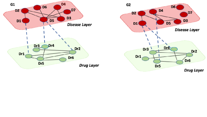
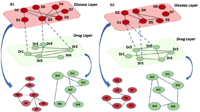
We explain our contribution using a toy example of a multilayer network with two layers without loss of generality; then we will discuss its formalization. Let us consider two multilayer input networks $G_{1}$, and $G_{2}$ presenting two layers: disease and drug, as reported in Figure 4. Node colors are used to distinguish different types of nodes belonging to two different types of layers. For simplicity, the two multilayer input networks have the same number of nodes.

Figure 4: Example of two Multilayer networks. The nodes represent a set of diseases and a set of drugs that belong to the Drug layer and the Disease layer. Please note that each layer networks has different edges; moreover, also, the inter-layer edges are different.

3.1 Step 1: Building of the multilayer alignment graph

3.2 Step (1.a). Building of intra-layer edges.

In the first step, MuLaN builds the MAG in two sub steps, initially it build all the alignment graphs for each layer $k$ (step 1.a, see Appendix for complete details), then it add all the inter-layer edges (Step 1.b).

3.3 Step (1.b). Building of inter-layer edges.

In the step 1.b, the algorithm adds the inter-layer edges. This step considers all the pairs of layers in the MAG. For each pair of layers ${k,t}$, it analyzes all the nodes. Each node of the graph into a single layer represents a pair of nodes in the corresponding of nodes. For each pair of nodes of the layers, MuLaN analyzes the corresponding layer of the input networks, and it inserts and weights the edges considering two conditions: match, or mismatch.

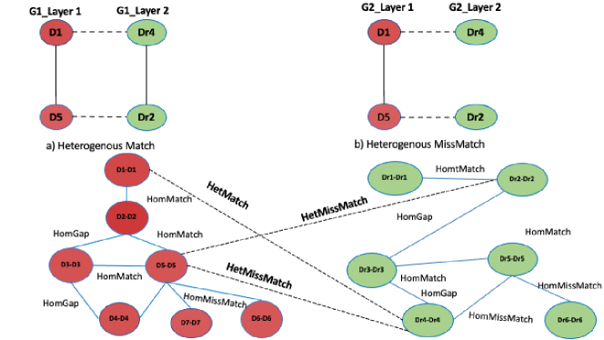
Let us consider the nodes of the alignment graphs 1 and the alignment graphs 2; in particular, let us analyze the pair of nodes $(D1-Dr4)$ and $(D5-Dr2)$ in Figure 4. To determine the presence of an edge, we consider the edges $(D1,Dr4)\in G_{1}$ network and $(D1,Dr4)\in G_{2}$ network. If $G_{1}$, and $G_{2}$ contains these nodes, and the nodes are adjacent, there is a match, that we call heterogeneous match because the node type are different, see Figure 5 (a).

Otherwise, if $G_{1}$, and $G_{2}$ contain these nodes, and the nodes are adjacent only in a single network, there is a mismatch which we call heterogeneous mismatch Figure 5 (b).

Finally, the algorithm assigns the weight to each edge as follows: heterogeneous match equal to 0.9, heterogeneous mismatch equal to 0.4. At the end of this step, the multilayer alignment graph is built.

Figure 5: Example of a heterogeneous match, mismatch and building of inter-layer Alignment Graph.

3.4 Step 2. Community Detection on the multilayer alignment graph

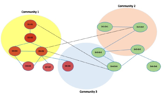
At this point, the algorithms analyzes the MAG to discover communities employing one of the previously introduced community detection methods [36, 37, 27, 38]. Since our methodology presents a general design, it is possible to mine the MAG by applying different community detection methods.

In the current version of MuLaN, we applied Louvain algorithm to mine the communities on the alignment graph. However, the user can choose the community detection algorithm by selecting among Louvain, Infomap and Greedy algorithms.

MuLaN generates three outputs: 1) a file containing the mined communities; 2) a file of the multilayer alignment graph represented as edge list, where the weight of the edge according to homogeneous/heterogeneous match, homogeneous/mismatch, homogeneous gap cases and type of layer; 3) a file containing the number of mined communities, the modularity value (where modularity is the measure related to the network structure that detects the density of connections within a module) and the run time (see an example of output at https://github.com/pietrocinaglia/mulan).

Figure 6: Example of Community Detection Extraction on inter-layer Alignment Graph.

3.5 Complexity of the algorithm

The asymptotic temporal complexity of the alignment process was estimated as $NxM$, with $N$ the number of interactions defined into the source network and $M$ that of the target one, calculated on the basis of the respective edge list.

The latter was designed as a multi-line adjacency list with data values, in order to store both node and edge attributes: node type, and the layer upon which (or between) the interaction is modeled. This approach allows us to have a flat view of the graph, which is therefore aligned using the same basic principles of alignment between static networks; its complexity will be proportionate to the resulting size.

It turns out to be quadratic, for multilayer networks consisting of edge lists with a same size ($N=M$).

4 Results and Discussion

As a proof of principle, we experimented MuLaN on two datasets, consisting of (i) ten synthetic multilayer networks, and (ii) one real multilayer network.

4.1 Dataset 1: Synthetic Networks

We build ten multilayer networks with two layers. Each layer is a Barabási-Albert network [39] having $1000$ nodes ($n=1000$) and $1000$ edges ($m=1$, with $m$ the number of edges to attach from a new node to existing ones).

The number of inter-edges was defined as $30\%$ (i.e., $300$) of the intra-edges, and these were randomly generated. The resulting edge list consisted of $2300$ interactions among $2000$ nodes, for the whole network.

According to the described approach, we modeled a set of $10$ initial multi-layer networks with $2$ layers, and five noisy versions for each one. The noisy version was built by removing $5\%$, $10\%$, $15\%$, $20\%$, and $25\%$ of interactions, randomly selected from the set of inter- and intra- edges. We have generated the pairs to be aligned by using the initial networks and the respective noisy versions.

4.2 Dataset 2: Real Network

We considered the following datasets of the Stanford Biomedical Network Dataset Collection (BioSNAP) [40]:

• Drug-Drug Interaction (DDI) network of interactions between drugs, approved by the U.S. Food and Drug Administration (FDA): $1514$ nodes and $48514$ edges.

• Disease-Disease (DD) network of interaction between inherited diseases: $6878$ nodes and $6877$ edges.

• Disease-Drug Association (DDA) network, a set of curated relationships between diseases and drugs: $5535$ disease nodes, $1662$ chemical nodes, and $466656$ edges.

We build a multilayer network with two layers obtained from the DDI and DD database. Then, we added inter-layer edges by considering the DDA database. Subsequently, a preprocessing was also performed to remove (i) zero degree nodes, (ii) duplicate edges, and (iii) objects outside the intersection set from the DDI, DD, and DDA networks. Finally, the resulting multilayer network consisted of $83,92$ nodes and $128,200$ interaction, of which $72,809$ inter-edges.

Similarly to our own synthetic networks, we generated five noised versions of the real network by removing $5\%$, $10\%$, $15\%$, $20\%$, and $25\%$ of interactions, randomly selected from the set of inter- and intra- edges.

4.3 Alignment Parameters

We set $\Delta$distance equal to 2, and following weights:

• Homogeneous Match : 1

• Homogeneous Mismatch: 0.5

• Homogeneous Gap: 0.2

• Heterogeneous Match: 0.9

• Heterogeneous Mismatch: 0.4.

4.4 Performance Evaluation

We evaluated MuLaN alignments by considering:

• the alignment of a network with respect to itself to show the ability to find known regions of similarity;

• the alignment of the network with respect to an altered version of the network obtained by adding different levels of noise ($5\%$, $10\%$, $15\%$, $20\%$, and $25\%$) by randomly removing edges from the network.

We aimed to demonstrate the ability of our algorithm to build high-quality alignments with edge conservation of about $90\%$.

The proposed solution aligned high-confidence synthetic networks to themselves and to their noisy counterparts. Overall, we computed a set of $60$ local alignments.

In addition to the experimentation on synthetic data, we aligned the high-confidence real network with itself and its noisy counterparts, by producing a total of $6$ local alignments.

All experiments have been conducted on a 64-bit workstation with the following specifications: AMD Ryzen 3 (2.6 GHz Dual-Core) and 8 GB of RAM.

MuLaN aligned two multilayer networks consisting of $2000$ nodes and $2298$ edges, each one, in $\sim 1.25$ seconds. To the latter, it was then necessary to include the time required by the individual methods for community detection; in details, Louvain, Greedy, and Infomap take $\sim 0.17$, $\sim 1.89$, and $\sim 14.09$ seconds, respectively.

According to our results, the most performing method in terms of modularity is Louvain (see Table 1 and Table 2); therefore, we defined the latter by default. However, Greedy and Infomap can be chosen as other options.

In order to evaluate the effectiveness of MuLaN, we generated the same local alignment built with Louvain by using Infomap and Greedy, and we analyzed the results. We selected those algorithms for the best and fast performance to extract community in multilayer network according to literature [18].

Since, to the best of our knowledge, MultiLoAl and its extension MuLaN are the only local alignment algorithms of multilayer networks in the literature, we evaluated the effectiveness of MuLaN, by comparing the results obtained with default MuLaN version, in which Louvain is used as community detection algorithm and other MuLaN versions in which are applied Infomap and Greedy algorithms.

Then, we measured the performance of the alignments built with different versions of MuLaN by evaluating the quality of the results. In particular, we measure the topological quality of alignments and the quality of communities found.

4.4.1 Topological quality

At first, the results are evaluated by analyzing the topological quality. We recall that intuitively an alignment is of high topological quality if it reconstructs the underlying true node mapping well (when such mapping is known) and if it conserves many edges. For example, for simple networks the ${F-NC}$ (F-score node correctness) is applied to measure the node correctness, and it is defined as $\frac{M\cap N}{N}$ where $M$ is the set of node pairs that are mapped under the true node mapping and $N$ the set of node pairs that are aligned under an alignment $f$.

Otherwise, NCV-G$S^{3}$ (high node coverage (NCV) and Generalized $S^{3}$ (G$S^{3}$)) is applied to measure the edge correctness, and it is defined as the geometric mean of high node coverage (NCV) and generalized $S^{3}$ (G$S^{3}$) measures. NCV is the percentage of nodes from $G_{1}$ and $G_{2}$ that are also in $G^{\prime}_{1}$ and $G^{\prime}_{2}$ and G$S^{3}$measures how well edges are conserved between $G^{\prime}_{1}$ and $G^{\prime}_{2}$ where $G_{1}$ and $G_{2}$ are two graphs and $G^{\prime}_{1}$ and $G^{\prime}_{2}$ are subgraphs of $G_{1}$ and $G_{2}$ that are induced by the mapping.

In a previous work ([14]), we extended such measures in the multilayer case, due to, to the best of our knowledge, there are not any other available measures.

In particular, we compute the multilayer ${F-NC_{m}}$ as the average of ${F-NC_{i}}$ estimated for each layer. Likewise, we compute the multilayer ${NCV-GS^{3}_{m}}$ as the average of ${NCV-GS^{3}_{m}}$ estimated for each layer.

Finally, we consider the edge correctness for the inter-layer edges. Without loss of information, we consider all the inter-layer edges as a whole, and we calculate the correctness of all the inter-layer edges as ${NCV-GS^{3}_{i}nter}$.

We computed multilayer ${NCV-GS^{3}_{m}}$ and multilayer ${F-NC_{m}}$ measures for all alignments built for each synthetic network and for real network by considering the intra-layer and inter-layer. Figure 7, Figure 8, Figure 9, Figure 10 report the results for synthetic multilayer networks, whereas Figure 11, Figure 12, Figure 13, Figure 14 report the results for real multilayer network. The Tables related to ${NCV-GS^{3}_{m}}$ and multilayer ${F-NC_{m}}$ measures for all alignments built for each synthetic network and for real network by considering the intra-layer and inter-layer are reported in appendix.

Figure 7: NCV-G$S^{3}$ values computed on intra-layer edges for all the local alignments built on synthetic networks by applying Louvain, Infomap, Greedy community detection algorithms.

Figure 8: NCV-G$S^{3}$ values computed on inter-edges for all the local alignments built on synthetic networks by applying Louvain, Infomap, Greedy community detection algorithms.

Figure 9: F-NC values computed on intra-layer edges for all the local alignments built on synthetic networks by applying Louvain, Infomap, Greedy community detection algorithms.

Figure 10: F-NC values computed on inter-layer edges for all the local alignments built on synthetic networks by applying Louvain, Infomap, Greedy community detection algorithms.

Figure 11: NCV-G$S^{3}$ values computed on intra-edges for all the local alignments built on real network by applying Louvain, Infomap, Greedy community detection algorithms.

Figure 12: NCV-G$S^{3}$ values computed on inter-edges for all the local alignments built on real network by applying Louvain, Infomap, Greedy community detection algorithms.

Figure 13: F-NC values computed on intra-edges for all the local alignments built on real network by applying Louvain, Infomap, Greedy community detection algorithms.

Figure 14: F-NC values computed on inter-edges for all the local alignments built on real network by applying Louvain, Infomap, Greedy community detection algorithms.

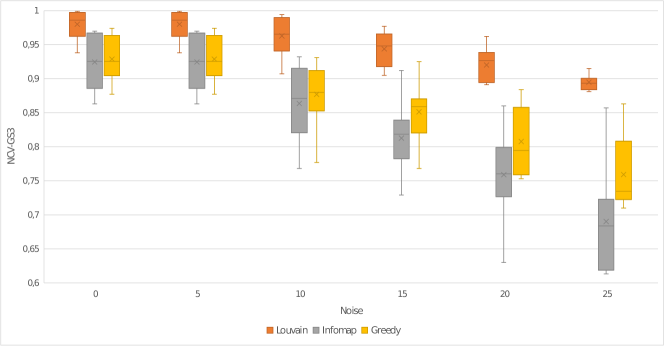
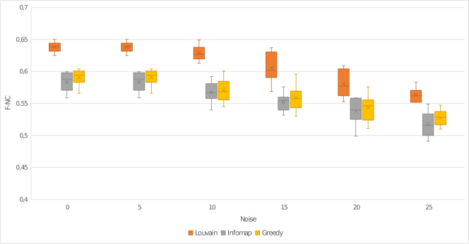
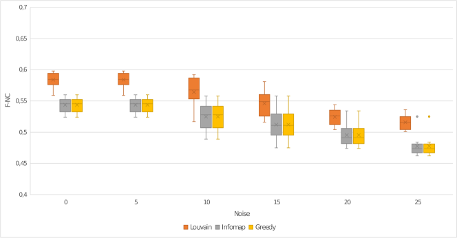
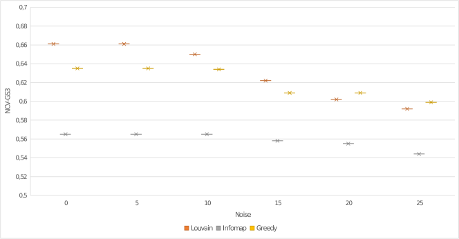
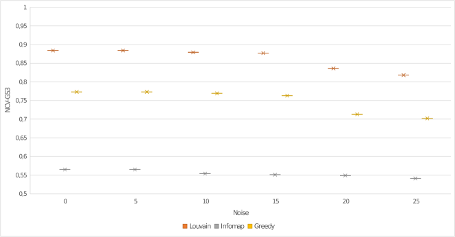
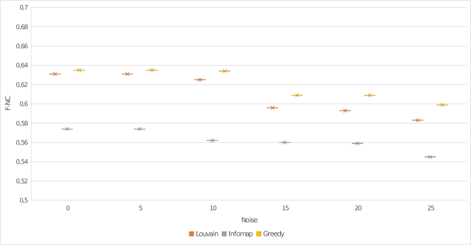
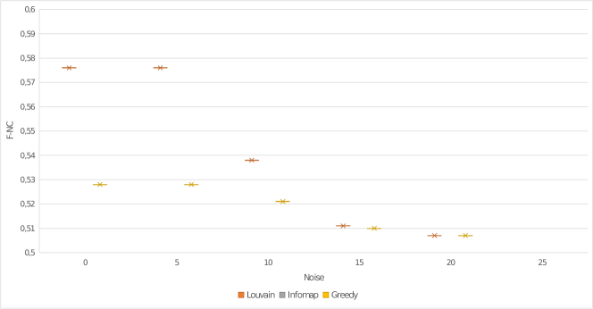
By analyzing the results, it is possible to notice that multilayer ${NCV-GS^{3}_{m}}$ and multilayer ${F-NC_{m}}$ values decrease by increasing noise level from 5 % to 25 %. The reduction of quality of the alignment is detected for different MuLaN versions applied on both synthetic network and real network. Otherwise, the results show that the quality of the alignment is greater when Louvain is applied to extract communities.

4.4.2 Community Quality

We also evaluated the quality of mined communities by considering i) the number of extracted communities and ii) the strength of the community structure by using the modularity [41] as a community quality metric. In detail, modularity is a measure related to the network structure that detects the density of connections within a module. The modularity can be either positive or negative, and positive values are indicative of the presence of community structure. Thus, a network with a high modularity score will have many connections within a community [41].

Thus, we first estimated the number of mined communities with Louvain, Infomap and Greedy, for each local alignment built on synthetic and real networks, then, we computed the modularity of the extracted communities.

Table 1 and Table 2 report the results obtained with different versions of the MuLaN algorithm for synthetic and real networks. In particular, for each network, the Tables report the number of the extracted communities and the modularity value for each community. The result shows that, all the community detection algorithms are able to mine more communities by aligning the original network with itself. Otherwise, the number of communities decreases on the alignment built with the synthetic counterparts with 5 %, 10%, 15%, 20% and 25% of added noise. Furthermore, it is possible to notice that Louvain is able to identify a higher number of communities in the multilayer network with respect to other community detection algorithms.

By analyzing the results, it is possible to see that the higher modularity values are obtained by applying Louvain as a community extraction algorithm. This means that Louvain is able to extract communities that reveal the relationships among nodes in various layers, with respect to other community detection algorithms.

Table 1: The Table reports for each synthetic network: the level of noise, number of Communities extracted and Modularity values by applying Louvain , Infomap , Greedy algorithms respectively.

Network	Noise	$\#$ Communities with Louvain	Modularity with Louvain	$\#$ Communities with Infomap	Modularity with Infomap	$\#$ Communities with Greedy	Modularity with Greedy
N1	0	37	0,844	28	0,839	38	0,844
	5	40	0,850	26	0,845	42	0,851
	10	40	0,857	29	0,855	44	0,857
	15	40	0,860	30	0,857	45	0,861
	20	42	0,872	28	0,867	46	0,873
	25	45	0,872	29	0,869	46	0,873
N2	0	39	0,840	27	0,836	40	0,841
	5	40	0,848	28	0,844	42	0,849
	10	40	0,859	32	0,857	42	0,859
	15	41	0,861	30	0,858	43	0,859
	20	41	0,870	27	0,856	46	0,861
	25	42	0,859	30	0,866	46	0,871
N3	0	38	0,843	28	0,840	37	0,843
	5	39	0,846	26	0,844	40	0,848
	10	37	0,868	31	0,854	42	0,856
	15	41	0,857	27	0,856	47	0,859
	20	43	0,859	28	0,865	44	0,867
	25	46	0,877	26	0,870	48	0,877
N4	0	41	0,843	29	0,839	41	0,843
	5	39	0,851	31	0,850	43	0,852
	10	42	0,859	29	0,856	40	0,859
	15	42	0,870	30	0,854	44	0,859
	20	43	0,867	32	0,862	50	0,867
	25	44	0,858	29	0,866	44	0,870
N5	0	38	0,842	29	0,839	41	0,841
	5	41	0,867	29	0,844	42	0,849
	10	42	0,849	30	0,852	43	0,854
	15	42	0,863	31	0,856	45	0,863
	20	42	0,874	34	0,863	47	0,867
	25	45	0,854	30	0,871	48	0,874
N6	0	40	0,841	27	27,000	39	0,841
	5	40	0,845	29	0,842	40	0,845
	10	42	0,856	27	0,842	46	0,856
	15	45	0,889	28	0,867	46	0,872
	20	46	0,872	35	0,887	50	0,888
	25	60	0,900	38	0,894	62	0,900
N7	0	37	0,845	29	0,841	39	0,844
	5	38	0,854	28	0,850	39	0,854
	10	43	0,867	30	0,859	43	0,867
	15	49	0,880	31	0,874	50	0,881
	20	52	0,904	35	0,889	55	0,893
	25	53	0,892	37	0,900	59	0,904
N8	0	40	0,843	27	0,840	41	0,844
	5	40	0,849	27	0,848	40	0,849
	10	39	0,861	28	0,856	43	0,861
	15	42	0,878	28	0,874	50	0,878
	20	46	0,887	29	0,879	58	0,888
	25	49	0,902	37	0,897	58	0,903
N9	0	36	0,852	24	0,839	40	0,844
	5	40	0,852	28	0,850	40	0,851
	10	39	0,861	30	0,858	44	0,861
	15	42	0,874	33	0,872	47	0,874
	20	44	0,887	32	0,883	47	0,886
	25	52	0,900	35	0,895	52	0,901
N10	0	38	0,840	29	0,838	41	0,841
	5	37	0,849	26	0,847	41	0,849
	10	39	0,861	28	0,858	42	0,862
	15	44	0,877	32	0,874	48	0,876
	20	52	0,890	33	0,884	56	0,890
	25	53	0,897	36	0,892	55	0,898

Table 2: The Table reports for the real network: the level of noise, number of Communities extracted and Modularity values by applying Louvain algorithm, Infomap algorithm, Greedy algorithm.

Network	Noise	$\#$ Communities with Louvain	Modularity with Generalized Louvain	$\#$ Communities with Infomap	Modularity with Infomap	$\#$ Communities with Greedy	Modularity with Greedy
N1	0	267	0.335	50	0.036	302	0.270
	5	268	0.331	49	0.034	301	0.268
	10	266	0.331	60	0.036	297	0.269
	15	260	0.331	46	0.035	340	0.250
	20	260	0.329	52	0.034	312	0.265
	25	263	0.327	57	0.031	307	0.260

4.4.3 Functional Quality Evaluation

Finally, we evaluate the functional quality of the results by considering the biological relevance of the extracted communities. For classical networks, the biological relevance evaluation consists in evaluating whether groups of related entities have a similar biological role or share functions. Since, MuLaN constructs the local alignment that includes associations between different entities, i.e. disease-drug, we conducted the evaluation differently. In particular, we evaluated the functional quality of local alignment, considering whether our algorithm is able to extract drug-disease associations still unobserved.

We recall that, drug-disease associations consist of the cases in which drugs affect disease. Thus, in research field, drug-disease associations may bring relevant information in the drug discovery, for example, the detection of convenient relations between drugs and diseases. The literature contain a large set of drug-disease associations already identified, however many associations are unobserved or not detected. In the rest of the paper, we refer to unobserved or not detected drug-disease associations as candidate drug-disease associations.

Starting from this consideration, our goal is to demonstrate that MuLaN is able to build a local alignment containing candidate drug-disease associations, and it is able to extract knowledge about the aligned multilayer networks.

For this aim, we consider the local alignment constructed by aligning the real network with its noisy counterpart at 25% (because it is the most different from the original network) and we analyze the drug-disease associations forming the extracted communities.

To evaluate whether the associations contained in the communities are known in the literature or still unobserved drug-disease associations, we used SCMFDD [42], a similarity constrained matrix factorization method for the drug-disease association prediction. SCMFDD reveals unobserved drug-disease associations by using drug features, disease semantic information and known associations incorporated into the matrix factorization frame (see [42] for complete details).

SCMFDD computes: i) the drug-drug similarities by using Jaccard index [43] taking into account diverse drug features (such as, targets, enzymes, pathways and drug-drug interactions), ii) the disease-disease semantic similarity by using MeSH information [44], iii) two low-rank feature matrices by applying a factorization on observed drug-disease associations matrix. Then, it uses an objective function based on Newton’s method [45] to compute a score representing the probability that a drug and a disease have an association (see [42] for complete details on SCMFDD). Thus, we applied SCMFDD to analyze each couple of drug-disease associations forming the community extracted with MuLaN. The results show that the extracted communities contain 46,498 candidate drug-disease associations. Among these, 711 drug-disease associations present a score greater than $0.5$. We reported candidate drug-disease associations with score equal to 1 in Table 3. The complete detected associations are available at https://github.com/pietrocinaglia/mulan).

Furthermore, we manually evaluated the candidate drug-disease associations by searching literature evidences. For example, by considering the drug-disease association Fenofibrate-Cholestasis, the works in [46, 47] report the effect of fenofibrate against cholestasis. In [47], Ghonem et al. discuss the effectiveness and well tolerability of Orlistat treatment for hyperglycemia. Also, [48] presents the successful use of rifampin in a patient with Stevens-Johnson syndrome. We list the literature evidence of the top 10 detected drugs-disease associations in Table 4.

In conclusion, the results demonstrate that our algorithm is capable of discovering candidate drug-disease associations and, consequently, of extracting new knowledge from multilayer networks.

Table 3: The Table reports an example of novel drug-disease associations contained in the local alignment built with MuLaN.

Drug ID	Drug Name	Disease ID	Disease Name	Score
DB01039	Fenofibrate	DOID:13580	Cholestasis	1
DB01083	Orlistat	DOID:4195	Hyperglycemia	1
DB01220	Rifaximin	DOID:0050426	Stevens-Johnson syndrome	1
DB00951	Isoniazid	DOID:2355	Anemia	1
DB00570	Vinblastine	DOID:2355	Anemia	1
DB01241	Gemfibrozil	DOID:13580	Cholestasis	1
DB01602	Bacampicillin	DOID:0050426	Stevens-Johnson syndrome	1
DB01042	Melphalan	DOID:987	Alopecia	1
DB00535	Cefdinir	DOID:13580	Cholestasis	1
DB01005	Hydroxyurea	DOID:1227	Neutropenia	1
DB01593	Zinc	DOID:2355	Anemia	1
DB00993	Azathioprine	DOID:1227	Neutropenia	1
DB02659	Cholic Acid	DOID:13580	Cholestasis	1
DB01103	Quinacrine	DOID:13580	Cholestasis	1
DB00970	Dactinomycin	DOID:1227	Neutropenia	1
DB00586	Diclofenac	DOID:2355	Anemia	1
DB00290	Bleomycin	DOID:2355	Anemia	1
DB00963	Bromfenac	DOID:13580	Cholestasis	1
DB01137	Levofloxacin	DOID:13580	Cholestasis	1
DB01262	Decitabine	DOID:299	Adenocarcinoma	1
DB01008	Busulfan	DOID:2355	Anemia	1
DB00549	Zafirlukast	DOID:13580	Cholestasis	1
DB00763	Methimazole	DOID:0050426	Stevens-Johnson syndrome	1
DB00591	Fluocinolone Ace	DOID:1555	Urticaria	1
DB01022	Phylloquinone	DOID:1555	Urticaria	1
DB00271	Diatrizoate	DOID:10763	Hypertension	1
DB01143	Amifostine	DOID:615	Leukopenia	1
DB01015	Sulfamethoxazole	DOID:1555	Urticaria	1
DB00984	Nandrolone phenp	DOID:10763	Hypertension	1
DB00296	Ropivacaine	DOID:10763	Hypertension	1
DB00205	Pyrimethamine	DOID:1588	Thrombocytopenia	1
DB01254	Dasatinib	DOID:13250	Diarrhea	1
DB00291	Chlorambucil	DOID:1588	Thrombocytopenia	1
DB00293	Raltitrexed	DOID:615	Leukopenia	1
DB01406	Danazol	DOID:2237	Hepatitis	1
DB00456	Cefalotin	DOID:1555	Urticaria	1
DB01138	Sulfinpyrazone	DOID:576	Proteinuria	1
DB00480	Lenalidomide	DOID:615	Leukopenia	1
DB01161	Chloroprocaine	DOID:10763	Hypertension	1
DB00287	Travoprost	DOID:10763	Hypertension	1
DB00121	Biotin	DOID:10763	Hypertension	1
DB00491	Miglitol	DOID:10763	Hypertension	1
DB00459	Acitretin	DOID:2237	Hepatitis	1
DB00905	Bimatoprost	DOID:10763	Hypertension	1
DB01288	Fenoterol	DOID:10763	Hypertension	1
DB04272	Citric acid	DOID:10763	Hypertension	1
DB01086	Benzocaine	DOID:1555	Urticaria	1

Table 4: Top 10 drug-disease associations contained in the local alignment built with MuLaN.

Drug Name	Disease Name	Evidence
Fenofibrate	Cholestasis	[46, 47]
Orlistat	Hyperglycemia	[49]
Rifaximin	Stevens-Johnson syndrome	[48]
Isoniazid	Anemia	[50]
Vinblastine	Anemia	[51]
Gemfibrozil	Cholestasis	[52]
Bacampicillin	Stevens-Johnson syndrome	[50]
Melphalan	Alopecia	[53]
Cefdinir	Cholestasis	[54]
Hydroxyurea	Neutropenia	[55]

4.4.4 MuLaN vs MultiLoAl

To clarify the need for developing an extended version of MultiLoAl, in this section, we present the comparison of MuLaN with MultiLoAl.The aim is to demonstrate that MuLaN reports the best performance to analyze multilayer networks with respect to previous version MultiLoAl. The dataset that we used for the comparison consists of ten synthetic multilayer networks and one real multilayer network used for MuLaN evaluation. Thus, we built the alignment of a network with respect to itself, and considering the alignment of a network with respect to an altered version by applying MultiLoAl. Our experimentation shows that MultiLoAl builds the alignment between two synthetic networks, having $2000$ nodes and $2298$ edges each one, in $\sim 120$ minutes, against the $\sim 1.42$ seconds required by MuLaN for the same operation.

Results show clearly that MuLaN outperforms MultiLoAl, in terms of memory efficiency and runtime.

5 Conclusions

Multilayer networks are a powerful tool for the modelling of complex data in biology and medicine. In this work, we focused on the problem of analysis of multilayer networks through the comparison of their internal structure, by applying Network Alignment algorithms. Since classical network alignment algorithms for simple networks do not perform well on multilayer networks, we presented a deep extension of a previously developed network alignment algorithm for multilayer network, named, MuLaN (Local Alignment Algorithm for Multilayer Networks). We tested it on ten synthetic multilayer networks and on a real multilayer network, and we evaluated the quality of results. Results confirm that MuLaN is able to build alignment with high topological quality. According to these analyses, we demonstrated the MuLaN methodology is suitable for the comparison and hence, the analysis of multilayer networks.

6 Competing interests

No competing interest is declared.

7 Author contributions statement

Conceptualization, PHG. and MM.; methodology, PHG, PC, and MM; software, PC, MM; data curation, MM and PC; writing–original draft preparation, MM, PC, PHG, and MC.; writing–review and editing, MM, PC, PHG and MC.; funding acquisition, MC. All authors have read and agreed to the published version of the manuscript.

8 Funding

This work was funded by the Next Generation EU - Italian NRRP, Mission 4, Component 2, Investment 1.5, call for the creation and strengthening of ’Innovation Ecosystems’, building ’Territorial R&D Leaders’ (Directorial Decree n. 2021/3277) - project Tech4You - Technologies for climate change adaptation and quality of life improvement, n. ECS0000009. This work reflects only the authors’ views and opinions, neither the Ministry for University and Research nor the European Commission can be considered responsible for them.

Appendix A Sample Appendix Section

This appendix present the process in which MuLaN builds the MAG and results of the computation of ${NCV-GS^{3}_{m}}$ and ${F-NC_{m}}$ measures for all alignments built for each synthetic network and for real network by considering the intra-layer and inter-layer.

A.1 Building of the Alignment Graph

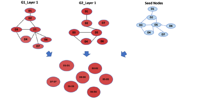
It receives as input two multilayer networks ($M_{1}$ and $M_{2}$) having the same number of layers $n$ and a multiset of seed nodes representing similarity between the node of each graph of the same layer $k$ of the two networks. We assume the existence of a bijective correlation among layers of the networks, so the layer $k$ of $M_{1}$ correspond to the layer $k$ of $M_{2}$. Starting from $M_{1}$ and $M_{2}$ and the multiset of seed nodes, in the step 1.a, MuLaN analyzes each pair of $k$ layers in $M_{1}$ and $M_{2}$ independently, see Figure 15. For each layer, MuLaN constructs an alignment graph on the basis of the strategy suggested in L-HetNetAligner. [12]. At this stage, MuLaN creates the nodes of the alignment graph. Each node $v_{al}\in V_{al}$ represents a match of nodes of the input graphs, so $V_{al}\subseteq V_{1}\times V_{2}$. Thus, the choice of node pairs is conducted by the input similarity relationships. Consequently, each node is matched with the most similar node of the other network on the same layer; and each node of the alignment graph represents a pair of similarity among nodes from the input networks, see Figure 16.

Figure 15: MuLaN separates the input networks according to the layer type.

Figure 16: Building of alignment graph for the disease layer of the two input multilayer networks: Node Definition. MuLaN takes the two networks in a layer and a subset of node pairs matched according to a similarity function and starts to build the alignment graph. In this step, the algorithm defines the nodes of the alignment graph represented by the pair matched nodes.

Figure 17: Example of homogeneous match, homogeneous mismatch and homogeneous gap and building of Alignment Graph.

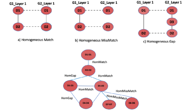
When all nodes have been inserted into the alignment graph, MuLaN adds the edges of the alignment graphs. For each pair of nodes, MuLaN analyzes the two input graphs, and it inserts and weights the edges considering three conditions: match, mismatch and gap. In the following, we present each condition. So, let us consider the nodes of the alignment graphs; in particular, let us analyze the pair of nodes $(D1-D1)$ and $(D2-D2)$ in Figure 4. To determine the presence of an edge, we we must consider the edges $(D1,D2)\in G_{1}$ network and the edges $(D1,D2)\in G_{2}$ network. If $G_{1}$, and $G_{2}$ contains these nodes, and the nodes are adjacent, we identify this condition as match, that, for convenience, we call homogeneous match, since the nodes of the two networks are of the same type i.e. disease, (see Figure 17 (a)).

Let us consider $\Delta=2$ as node distance, i.e. the length of the shortest connecting path threshold to discriminate between gaps and mismatches. Let us consider the pair of nodes $(D1-D1)$ and $(D2-D2)$ (Figure 17 (b)). $G_{1}$ contains the edges $(D1,D2)$, whereas the nodes $(D1-D1)$ are disconnected in $G_{2}$. We identify this condition as mismatch that we call homogeneous mismatch. Let us consider the pair of nodes $(D1-D1)$ and $(D2-D2)$ (Figure 17 (c)). $G_{1}$ contains the edges $(D1,D2)$, whereas the nodes $(D1-D1)$ have a distance equal to 2 in $G_{2}$. We identify this condition as gap that we call homogeneous gap.

Once the edges of the alignment graph are added, a weight is assigned to each edge by applying an ad-hoc scoring function $F$ and the gap threshold $\Delta$. The function assigns a highest score to the matches, respect to mismatch and gaps. The kind of scoring function has a large significance on the resulting alignment graph and on the alignment itself. The algorithm enables the user to choose several values of $\Delta$ to optimize the quality of results. In this work we set the weight assigned to each edge as follows: homogeneous match equal to $1$, homogeneous mismatch equal to $0.5$, homogeneous gap equal to $0.2$.

A.2 Topological quality

Table 5, Table 6, Table 7, Table 8 report the results for synthetic multilayer networks, whereas Table 9, Table 10, Table 11, Table 12 report the results for real multilayer network.

Table 5: NCV-G$S^{3}$ values computed on intra-layer edges for all the local alignments built on synthetic networks by applying Louvain, Infomap, Greedy community detection algorithms.

Network	Noise	NCV-G$S^{3}$ with Louvain	NCV-G$S^{3}$ with Infomap	NCV-G$S^{3}$ with Greedy
N1	0	0.631	0.574	0.604
	5	0.631	0.574	0.604
	10	0.625	0.562	0.589
	15	0.596	0.56	0.557
	20	0.593	0.559	0.55
	25	0.583	0.545	0.537
N2	0	0.635	0.599	0.6
	5	0.635	0.599	0.6
	10	0.628	0.581	0.583
	15	0.592	0.54	0.58
	20	0.573	0.527	0.576
	25	0.559	0.527	0.533
N3	0	0.648	0.587	0.595
	5	0.648	0.587	0.595
	10	0.643	0.572	0.557
	15	0.629	0.544	0.53
	20	0.553	0.532	0.524
	25	0.552	0.53	0.518
N4	0	0.641	0.598	0.594
	5	0.641	0.598	0.594
	10	0.621	0.592	0.583
	15	0.61	0.554	0.566
	20	0.609	0.549	0.545
	25	0.57	0.502	0.52
N5	0	0.643	0.588	0.571
	5	0.643	0.588	0.571
	10	0.624	0.565	0.554
	15	0.569	0.559	0.545
	20	0.568	0.559	0.511
	25	0.552	0.549	0.51
N6	0	0.632	0.559	0.589
	5	0.632	0.559	0.589
	10	0.613	0.54	0.577
	15	0.587	0.539	0.565
	20	0.581	0.499	0.564
	25	0.57	0.495	0.539
N7	0	0.639	0.6	0.604
	5	0.639	0.6	0.604
	10	0.635	0.581	0.601
	15	0.607	0.576	0.596
	20	0.563	0.52	0.553
	25	0.552	0.517	0.527
N8	0	0.625	0.578	0.587
	5	0.625	0.578	0.587
	10	0.616	0.569	0.545
	15	0.594	0.556	0.538
	20	0.559	0.548	0.524
	25	0.558	0.491	0.513
N9	0	0.638	0.561	0.566
	5	0.638	0.561	0.566
	10	0.636	0.552	0.556
	15	0.635	0.532	0.549
	20	0.604	0.527	0.548
	25	0.572	0.51	0.547
N10	0	0.65	0.592	0.6
	5	0.65	0.592	0.6
	10	0.649	0.56	0.56
	15	0.637	0.56	0.559
	20	0.604	0.558	0.543
	25	0.566	0.515	0.53

Table 6: NCV-G$S^{3}$ values computed on inter-layer edges for all the local alignments built on synthetic networks by applying Louvain, Infomap, Greedy community detection algorithms.

Network	Noise	NCV-G$S^{3}$ with Louvain	NCV-G$S^{3}$ with Infomap	NCV-G$S^{3}$ with Greedy
N1	0	0.598	0.547	0.545
	5	0.598	0.547	0.545
	10	0.586	0.537	0.506
	15	0.527	0.52	0.5
	20	0.504	0.487	0.5
	25	0.501	0.475	0.486
N2	0	0.583	0.524	0.546
	5	0.583	0.524	0.546
	10	0.563	0.504	0.523
	15	0.555	0.502	0.516
	20	0.542	0.484	0.508
	25	0.536	0.472	0.492
N3	0	0.589	0.544	0.577
	5	0.589	0.544	0.577
	10	0.589	0.526	0.556
	15	0.567	0.525	0.545
	20	0.52	0.503	0.539
	25	0.516	0.48	0.527
N4	0	0.593	0.55	0.541
	5	0.593	0.55	0.541
	10	0.592	0.539	0.495
	15	0.581	0.532	0.494
	20	0.507	0.515	0.482
	25	0.504	0.477	0.482
N5	0	0.598	0.532	0.567
	5	0.598	0.532	0.567
	10	0.571	0.508	0.548
	15	0.546	0.5	0.498
	20	0.532	0.493	0.488
	25	0.525	0.484	0.483
N6	0	0.583	0.539	0.574
	5	0.583	0.539	0.574
	10	0.564	0.509	0.549
	15	0.552	0.475	0.516
	20	0.544	0.475	0.516
	25	0.525	0.464	0.489
N7	0	0.559	0.551	0.574
	5	0.559	0.551	0.574
	10	0.517	0.489	0.522
	15	0.516	0.481	0.512
	20	0.514	0.474	0.496
	25	0.513	0.462	0.491
N8	0	0.586	0.557	0.577
	5	0.586	0.557	0.577
	10	0.571	0.549	0.576
	15	0.537	0.528	0.556
	20	0.533	0.489	0.531
	25	0.519	0.468	0.512
N9	0	0.576	0.56	0.574
	5	0.576	0.56	0.574
	10	0.564	0.558	0.555
	15	0.558	0.558	0.555
	20	0.533	0.534	0.545
	25	0.515	0.525	0.487
N10	0	0.576	0.533	0.532
	5	0.576	0.533	0.532
	10	0.524	0.53	0.519
	15	0.521	0.5	0.519
	20	0.515	0.499	0.493
	25	0.504	0.468	0.49

Table 7: F-NC values computed on intra-layer edges for all the local alignments built on synthetic networks by applying Louvain, Infomap, Greedy community detection algorithms.

Network	Noise	F-NC with Louvain	F-NC with Infomap	F-NC with Greedy
N1	0	0.999	0.934	0.974
	5	0.999	0.934	0.974
	10	0.994	0.913	0.927
	15	0.961	0.912	0.889
	20	0.926	0.86	0.87
	25	0.896	0.857	0.863
N2	0	0.986	0.863	0.971
	5	0.986	0.863	0.971
	10	0.957	0.768	0.907
	15	0.951	0.729	0.857
	20	0.927	0.63	0.76
	25	0.896	0.618	0.71
N3	0	0.981	0.87	0.93
	5	0.981	0.87	0.93
	10	0.96	0.836	0.859
	15	0.919	0.821	0.858
	20	0.902	0.741	0.804
	25	0.883	0.613	0.799
N4	0	0.997	0.891	0.921
	5	0.997	0.891	0.921
	10	0.992	0.889	0.879
	15	0.945	0.835	0.825
	20	0.927	0.791	0.785
	25	0.893	0.683	0.747
N5	0	0.963	0.951	0.92
	5	0.963	0.951	0.92
	10	0.907	0.853	0.777
	15	0.905	0.852	0.768
	20	0.895	0.82	0.753
	25	0.894	0.684	0.733
N6	0	0.938	0.917	0.877
	5	0.938	0.917	0.877
	10	0.928	0.905	0.868
	15	0.914	0.816	0.86
	20	0.891	0.699	0.854
	25	0.881	0.619	0.724
N7	0	0.998	0.967	0.908
	5	0.998	0.967	0.908
	10	0.985	0.922	0.906
	15	0.977	0.828	0.861
	20	0.938	0.765	0.846
	25	0.892	0.764	0.723
N8	0	0.96	0.97	0.932
	5	0.96	0.97	0.932
	10	0.945	0.932	0.881
	15	0.928	0.797	0.864
	20	0.893	0.755	0.755
	25	0.884	0.709	0.721
N9	0	0.992	0.916	0.961
	5	0.992	0.916	0.961
	10	0.989	0.786	0.931
	15	0.974	0.739	0.925
	20	0.962	0.736	0.884
	25	0.915	0.651	0.836
N10	0	0.986	0.967	0.894
	5	0.986	0.967	0.894
	10	0.971	0.832	0.834
	15	0.963	0.798	0.806
	20	0.94	0.792	0.766
	25	0.914	0.704	0.736

Table 8: F-NC values computed on inter-layer edges for all the local alignments built on synthetic networks by applying Louvain, Infomap, Greedy community detection algorithms.

Network	Noise	F-NC with Louvain	F-NC with Infomap	F-NC with Greedy
N1	0	0.771	0.706	0.757
	5	0.771	0.706	0.757
	10	0.77	0.671	0.7
	15	0.717	0.64	0.678
	20	0.659	0.614	0.652
	25	0.645	0.604	0.592
N2	0	0.796	0.698	0.743
	5	0.796	0.698	0.743
	10	0.723	0.695	0.7
	15	0.69	0.68	0.691
	20	0.674	0.605	0.681
	25	0.607	0.569	0.623
N3	0	0.793	0.696	0.728
	5	0.793	0.696	0.728
	10	0.697	0.692	0.704
	15	0.677	0.661	0.699
	20	0.668	0.65	0.69
	25	0.614	0.566	0.585
N4	0	0.763	0.666	0.775
	5	0.763	0.666	0.775
	10	0.724	0.621	0.74
	15	0.679	0.621	0.698
	20	0.639	0.588	0.653
	25	0.6	0.586	0.601
N5	0	0.745	0.732	0.775
	5	0.745	0.732	0.775
	10	0.702	0.697	0.683
	15	0.666	0.694	0.607
	20	0.658	0.628	0.603
	25	0.616	0.572	0.585
N6	0	0.748	0.678	0.745
	5	0.748	0.678	0.745
	10	0.738	0.678	0.727
	15	0.697	0.642	0.625
	20	0.62	0.627	0.603
	25	0.612	0.591	0.593
N7	0	0.735	0.718	0.777
	5	0.735	0.718	0.777
	10	0.728	0.67	0.713
	15	0.692	0.659	0.698
	20	0.661	0.592	0.631
	25	0.608	0.561	0.602
N8	0	0.758	0.719	0.753
	5	0.758	0.719	0.753
	10	0.739	0.7	0.743
	15	0.718	0.695	0.735
	20	0.707	0.669	0.699
	25	0.627	0.597	0.683
N9	0	0.712	0.708	0.763
	5	0.712	0.708	0.763
	10	0.665	0.687	0.735
	15	0.659	0.685	0.724
	20	0.658	0.669	0.714
	25	0.621	0.619	0.666
N10	0	0.765	0.724	0.764
	5	0.765	0.724	0.764
	10	0.754	0.628	0.761
	15	0.692	0.612	0.725
	20	0.681	0.571	0.712
	25	0.618	0.542	0.691

Table 9: NCV-G$S^{3}$ values computed on intra-layer edges for all the local alignments built on real network by applying Louvain, Infomap, Greedy community detection algorithms.

Network	Noise	NCV-G$S^{3}$ with Louvain	NCV-G$S^{3}$ with Infomap	NCV-G$S^{3}$ with Greedy
N1	0	0.884	0.565	0.773
	5	0.884	0.565	0.773
	10	0.879	0.554	0.769
	15	0.877	0.551	0.763
	20	0.836	0.549	0.713
	25	0.818	0.541	0.702

Table 10: NCV-G$S^{3}$ values computed on inter-layer edges for all the local alignments built on real network by applying Louvain, Infomap, Greedy community detection algorithms.

Network	Noise	NCV-G$S^{3}$ with Louvain	NCV-G$S^{3}$ with Infomap	NCV-G$S^{3}$ with Greedy
Real Network	0	0.661	0.565	0.635
	5	0.661	0.565	0.635
	10	0.65	0.565	0.634
	15	0.622	0.558	0.609
	20	0.602	0.555	0.609
	25	0.592	0.544	0.599

Table 11: F-NC values computed on intra-layer edges forfor all the local alignments built on real network by applying Louvain, Infomap, Greedy community detection algorithms.

Network	Noise	F-NC with Louvain	F-NC with Infomap	F-NC with Greedy
Real Network	0	0.661	0.565	0.635
	5	0.661	0.565	0.635
	10	0.65	0.565	0.634
	15	0.622	0.558	0.609
	20	0.602	0.555	0.609
	25	0.592	0.544	0.599

Table 12: F-NC values computed on inter-layer edges for all the local alignments built on real network by applying Louvain, Infomap, Greedy community detection algorithms.

Network	Noise	F-NC with Louvain	F-NC with Infomap	F-NC with Greedy
Real Network	0	0.576	0.497	0.528
	5	0.576	0.497	0.528
	10	0.538	0.486	0.521
	15	0.511	0.484	0.51
	20	0.507	0.478	0.507
	25	0.498	0.46	0.486

References

- [1] M. Cannataro, P. H. Guzzi, P. Veltri, Protein-to-protein interactions: Technologies, databases, and algorithms, ACM Computing Surveys (CSUR) 43 (1) (2010) 1–36.
- [2] A.-L. Barabasi, Z. N. Oltvai, Network biology: understanding the cell’s functional organization, Nature reviews genetics 5 (2) (2004) 101–113.
- [3] S. Gu, M. Jiang, P. H. Guzzi, T. Milenković, Modeling multi-scale data via a network of networks, Bioinformatics 38 (9) (2022) 2544–2553.
- [4] M. Milano, P. H. Guzzi, O. Tymofieva, D. Xu, C. Hess, P. Veltri, M. Cannataro, An extensive assessment of network alignment algorithms for comparison of brain connectomes, BMC bioinformatics 18 (2017) 31–45.
- [5] R. Dondi, M. M. Hosseinzadeh, P. H. Guzzi, A novel algorithm for finding top-k weighted overlapping densest connected subgraphs in dual networks, Applied Network Science 6 (1) (2021) 40.
- [6] N. Eskandarzade, A. Ghorbani, S. Samarfard, J. Diaz, P. H. Guzzi, N. Fariborzi, A. Tahmasebi, K. Izadpanah, Network for network concept offers new insights into host-sars-cov-2 protein interactions and potential novel targets for developing antiviral drugs, Computers in biology and medicine 146 (2022) 105575.
- [7] A. Tagarelli, A. Amelio, F. Gullo, Ensemble-based community detection in multilayer networks, Data Mining and Knowledge Discovery 31 (5) (2017) 1506–1543.
- [8] Z. Hammoud, F. Kramer, Multilayer networks: aspects, implementations, and application in biomedicine, Big Data Analytics 5 (1) (2020) 1–18.
- [9] M. Kivelä, A. Arenas, M. Barthelemy, J. P. Gleeson, Y. Moreno, M. A. Porter, Multilayer networks, Journal of complex networks 2 (3) (2014) 203–271.
- [10] P. Cinaglia, M. Cannataro, Network alignment and motif discovery in dynamic networks, Network Modeling Analysis in Health Informatics and Bioinformatics 11 (10 2022). doi:10.1007/s13721-022-00383-1.
- [11] P. H. Guzzi, G. Agapito, M. Cannataro, coresnp: Parallel processing of microarray data, IEEE Transactions on Computers 63 (12) (2013) 2961–2974.
- [12] M. Milano, T. Milenković, M. Cannataro, P. H. Guzzi, L-hetnetaligner: a novel algorithm for local alignment of heterogeneous biological networks, Scientific reports 10 (1) (2020) 1–20.
- [13] J. Kumar Das, G. Tradigo, P. Veltri, P. H Guzzi, S. Roy, Data science in unveiling covid-19 pathogenesis and diagnosis: evolutionary origin to drug repurposing, Briefings in Bioinformatics 22 (2) (2021) 855–872.
- [14] M. Milano, P. H. Guzzi, M. Cannataro, Design and implementation of a new local alignment algorithm for multilayer networks, Entropy 24 (9) (2022) 1272.
- [15] I. S. Jutla, L. G. Jeub, P. J. Mucha, et al., A generalized louvain method for community detection implemented in matlab, URL http://netwiki. amath. unc. edu/GenLouvain (2011).
- [16] M. De Domenico, A. Lancichinetti, A. Arenas, M. Rosvall, Identifying modular flows on multilayer networks reveals highly overlapping organization in interconnected systems, Physical Review X 5 (1) (2015) 011027.
- [17] M. E. Newman, Fast algorithm for detecting community structure in networks, Physical review E 69 (6) (2004) 066133.
- [18] M. Magnani, O. Hanteer, R. Interdonato, L. Rossi, A. Tagarelli, Community detection in multiplex networks, ACM Computing Surveys (CSUR) 54 (3) (2021) 1–35.
- [19] P. H. Guzzi, T. Milenković, Survey of local and global biological network alignment: the need to reconcile the two sides of the same coin, Briefings in bioinformatics 19 (3) (2018) 472–481.
- [20] G. Ciriello, M. Mina, P. H. Guzzi, M. Cannataro, C. Guerra, Alignnemo: a local network alignment method to integrate homology and topology, PloS one 7 (6) (2012) e38107.
- [21] M. Mina, P. H. Guzzi, Improving the robustness of local network alignment: design and extensive assessmentof a markov clustering-based approach, IEEE/ACM Transactions on Computational Biology and Bioinformatics 11 (3) (2014) 561–572.
- [22] A. J. Enright, S. Van Dongen, C. A. Ouzounis, An efficient algorithm for large-scale detection of protein families, Nucleic acids research 30 (7) (2002) 1575–1584.
-
[23]
M. Milano, W. B. Hayes, P. Veltri, M. Cannataro, P. H. Guzzi,
Sl-glalign: improving local
alignment of biological networks through simulated annealing, Netw. Model.
Anal. Health Informatics Bioinform. 9 (1) (2020) 10.
doi:10.1007/s13721-019-0214-4.
URL https://doi.org/10.1007/s13721-019-0214-4 -
[24]
R. Sharan, T. Ideker,
Modeling cellular
machinery through biological network comparison., Nature biotechnology
24 (4) (2006) 427–33.
doi:10.1038/nbt1196.
URL http://www.ncbi.nlm.nih.gov/pubmed/16601728 - [25] R. A. Pache, A. Ceol, P. Aloy, Netaligner, a network alignment server to compare complexes, pathways and whole interactomes, Nucleic acids research 40 (W1) (2012) W157–W161.
- [26] P. Cinaglia, M. Cannataro, A method based on temporal embedding for the pairwise alignment of dynamic networks, Entropy 25 (4) (2023). doi:10.3390/e25040665.
- [27] P. H. Guzzi, E. Salerno, G. Tradigo, P. Veltri, Extracting dense and connected communities in dual networks: an alignment based algorithm, IEEE Access 8 (2020) 162279–162289.
- [28] Y. Ren, A. Sarkar, P. Veltri, A. Ay, A. Dobra, T. Kahveci, Pattern discovery in multilayer networks, IEEE/ACM Transactions on Computational Biology and Bioinformatics 19 (2) (2021) 741–752.
- [29] S. Fortunato, D. Hric, Community detection in networks: A user guide, Physics reports 659 (2016) 1–44.
- [30] A. Lancichinetti, S. Fortunato, Consensus clustering in complex networks, Scientific reports 2 (1) (2012) 1–7.
- [31] V. Gligorijević, Y. Panagakis, S. Zafeiriou, Fusion and community detection in multi-layer graphs, in: 2016 23rd International Conference on Pattern Recognition (ICPR), IEEE, 2016, pp. 1327–1332.
- [32] M. Rosvall, C. T. Bergstrom, Maps of random walks on complex networks reveal community structure, Proceedings of the national academy of sciences 105 (4) (2008) 1118–1123.
- [33] M. Berlingerio, F. Pinelli, F. Calabrese, Abacus: frequent pattern mining-based community discovery in multidimensional networks, Data Mining and Knowledge Discovery 27 (3) (2013) 294–320.
- [34] N. Afsarmanesh Tehrani, M. Magnani, Partial and overlapping community detection in multiplex social networks, in: International conference on social informatics, Springer, 2018, pp. 15–28.
- [35] O. Boutemine, M. Bouguessa, Mining community structures in multidimensional networks, ACM Transactions on Knowledge Discovery from Data (TKDD) 11 (4) (2017) 1–36.
- [36] J. Kim, J.-G. Lee, Community detection in multi-layer graphs: A survey, ACM SIGMOD Record 44 (3) (2015) 37–48.
- [37] S. Paul, Y. Chen, Spectral and matrix factorization methods for consistent community detection in multi-layer networks, The Annals of Statistics 48 (1) (2020) 230–250.
- [38] X. Huang, D. Chen, T. Ren, D. Wang, A survey of community detection methods in multilayer networks, Data Mining and Knowledge Discovery 35 (1) (2021) 1–45.
- [39] A. L. Barabási, Z. N. Oltvai, Network biology: understanding the cell’s functional organization, Nat Rev Genet 5 (2) (2004) 101–113.
- [40] M. Zitnik, R. Sosič, S. Maheshwari, J. Leskovec, BioSNAP Datasets: Stanford biomedical network dataset collection, http://snap.stanford.edu/biodata (Aug. 2018).
- [41] M. E. Newman, Modularity and community structure in networks, Proceedings of the national academy of sciences 103 (23) (2006) 8577–8582.
- [42] W. Zhang, X. Yue, W. Lin, W. Wu, R. Liu, F. Huang, F. Liu, Predicting drug-disease associations by using similarity constrained matrix factorization, BMC bioinformatics 19 (2018) 1–12.
- [43] R. Real, J. M. Vargas, The probabilistic basis of jaccard’s index of similarity, Systematic biology 45 (3) (1996) 380–385.
- [44] P. Xuan, K. Han, M. Guo, Y. Guo, J. Li, J. Ding, Y. Liu, Q. Dai, J. Li, Z. Teng, et al., Prediction of micrornas associated with human diseases based on weighted k most similar neighbors, PloS one 8 (8) (2013) e70204.
- [45] A. S. Berahas, R. H. Byrd, J. Nocedal, Derivative-free optimization of noisy functions via quasi-newton methods, SIAM Journal on Optimization 29 (2) (2019) 965–993.
- [46] M. Dai, J. Yang, M. Xie, J. Lin, M. Luo, H. Hua, G. Xu, H. Lin, D. Song, Y. Cheng, et al., Inhibition of jnk signalling mediates ppar-dependent protection against intrahepatic cholestasis by fenofibrate, British journal of pharmacology 174 (18) (2017) 3000–3017.
- [47] N. S. Ghonem, D. N. Assis, J. L. Boyer, Fibrates and cholestasis, Hepatology 62 (2) (2015) 635–643.
- [48] J. R. Yonkof, D. E. Tapke, C. C. Fox, P. U. Ogbogu, Successful use of rifampin in a patient with stevens-johnson syndrome to rifabutin, Annals of Allergy, Asthma & Immunology 124 (6) (2020) 624–626.
- [49] M. S. Ganjayi, R. S. Karunakaran, S. Gandham, B. Meriga, Quercetin-3-o-rutinoside from moringa oleifera downregulates adipogenesis and lipid accumulation and improves glucose uptake by activation of ampk/glut-4 in 3t3-l1 cells, Revista Brasileira de Farmacognosia (2023) 1–10.
- [50] A. Romano, A. Oussalah, C. Chery, R.-M. Guéant-Rodriguez, F. Gaeta, J.-A. Cornejo-Garcia, P. Rouyer, T. Josse, C. Mayorga, M.-J. Torres, et al., Next-generation sequencing and genotype association studies reveal the association of hla-drb3* 02: 02 with delayed hypersensitivity to penicillins, Allergy 77 (6) (2022) 1827–1834.
- [51] A. Vagrecha, L. C. Wolfe, Extracorpuscular hemolytic anemia, in: Lanzkowsky’s Manual of Pediatric Hematology and Oncology, Elsevier, 2022, pp. 151–159.
- [52] Q. Yang, X. Wu, Z. Pan, R. Guan, P. Yang, Y. Liu, X. Yang, W. Du, J. Liang, J. Hu, et al., Integration of pharmacodynamics, network pharmacology and metabolomics to elucidate effect and mechanism of artemisia capillaris thunb. in the treatment of jaundice, Journal of Ethnopharmacology 303 (2023) 115943.
- [53] E. Gurevich, M. Hayoz, Y. Aebi, C. R. Largiadèr, B. Mansouri Taleghani, U. Bacher, T. Pabst, Comparison of melphalan combined with treosulfan or busulfan as high-dose chemotherapy before autologous stem cell transplantation in aml, Cancers 14 (4) (2022) 1024.
- [54] S. R. Phillips, S. Groome, C. Borja, Beta-lactams and tetracyclines, in: Side Effects of Drugs Annual, Vol. 44, Elsevier, 2022, pp. 261–274.
- [55] S. Akram, S. A. K. Khattak, M. A. Khan, Efficacy and safety of hydroxyurea as adjuvant therapy in pediatric patients of transfusion-dependent beta-thalassemia major at zhob, balochistan, Cureus 14 (7) (2022).