Multi-Grade Deep Learning for Partial Differential Equations with Applications to the Burgers Equation

Abstract

We develop in this paper a multi-grade deep learning method for solving nonlinear partial differential equations (PDEs). Deep neural networks (DNNs) have received super performance in solving PDEs in addition to their outstanding success in areas such as natural language processing, computer vision, and robotics. However, training a very deep network is often a challenging task. As the number of layers of a DNN increases, solving a large-scale non-convex optimization problem that results in the DNN solution of PDEs becomes more and more difficult, which may lead to a decrease rather than an increase in predictive accuracy. To overcome this challenge, we propose a two-stage multi-grade deep learning (TS-MGDL) method that breaks down the task of learning a DNN into several neural networks stacked on top of each other in a staircase-like manner. This approach allows us to mitigate the complexity of solving the non-convex optimization problem with large number of parameters and learn residual components left over from previous grades efficiently. We prove that each grade/stage of the proposed TS-MGDL method can reduce the value of the loss function and further validate this fact through numerical experiments. Although the proposed method is applicable to general PDEs, implementation in this paper focuses only on the 1D, 2D, and 3D viscous Burgers equations. Experimental results show that the proposed two-stage multi-grade deep learning method enables efficient learning of solutions of the equations and outperforms existing single-grade deep learning methods in predictive accuracy. Specifically, the predictive errors of the single-grade deep learning are larger than those of the TS-MGDL method in 26-60, 4-31 and 3-12 times, for the 1D, 2D, and 3D equations, respectively.

68T07, 76L05, 65M99

1 Introduction

Over the last decade, the use of deep neural networks (DNNs) has achieved tremendous success in various fields of science and technology. In areas such as natural language processing, computer vision, and robotics, deep learning has surpassed traditional artificial intelligence [15, 28]. Using multiple layers, DNNs can effectively discover multi-scale features and representations in input data. Besides its applications in the traditional machine learning field, DNNs have been widely employed in many domains, including physics [12, 23], scientific computing [9], and finance [11]. The great successes of DNNs are, to a great extent, due to their mighty expressiveness in representing a function. Understanding the mathematical properties of DNNs has become a current research focus in the area of applied mathematics [10, 21, 26, 35, 36, 37].

Partial differential equations (PDEs) have numerous applications in modern science and engineering. Obtaining accurate solutions for nonlinear PDEs remains a challenging and active research area. Traditional numerical methods, such as finite difference [8, 22], finite elements [5], finite volume schemes [6, 7, 17], spectral methods [25], and meshless methods [1] have achieved impressive success in solving various PDEs. However, traditional numerical methods often require specific techniques for different problems and can be computationally expensive when solving complex PDEs, especially those in irregular or high-dimensional domains and those with singularities in their solutions. Moreover, traditional numerical methods suffer from the curse of dimensionality.

Neural network-based methods have attracted great attention in numerical solutions of PDEs. The basic idea of these methods is to use neural networks to represent their unknown solutions. These methods take advantage of the power of DNNs to approximate solutions of PDEs. The PDEs are typically encoded as constraints or loss functions, which the DNNs are trained to minimize the loss function. DNNs can serve as a universal solver for different problems and do not require mesh generation, making them suitable for solving problems in high-dimensional spaces and complex domains. In recent years, various DNN-based methods have been proposed for solving PDEs, including physics-informed neural networks (PINN) [24], deep Ritz [13], deep Galerkin method [27], convolutional neural networks [14], generative adversarial networks [2], multi-scale DNN [29], and sparse DNN [34]. DNN-based methods for PDEs have been successfully applied in various fields such as fluid dynamics, structural mechanics, and molecular dynamics.

Despite DNNs’ great successes in solving PDEs, there are still several challenges that need to be addressed. Typically, a DNN employs a single optimization method to train all of its parameters. However, as the number of layers of the network increases, it becomes increasingly challenging to solve the associated minimization problem, requiring larger amounts of data and computational power. Additionally, deeper networks tend to suffer from overfitting, leading to reduced accuracy and generalization performance.

In this paper, we propose a two-stage (TS) multi-grade deep learning (MGDL) method to address the limitations of DNNs when used in solving PDEs. The MGDL method was previously proposed in [32, 33] in a general setting. The main idea of the MGDL is based on residual learning, where each grade stacks additional layers on top of the previous grade (with fixed parameters) to learn the residual of the approximation. The original training of multi-grade DNN is conducted grade by grade. For each grade, one only needs to solve a relatively small-scale optimization problem to learn a shallow DNN. To avoid the MGDL method getting trapped in an unwanted local minimizer, we propose a two-stage training strategy for the multi-grade neural network solution of PDEs. In the first stage, we train the multi-grade deep network incrementally, one grade at a time. In the second stage, we unfreeze the parameters of certain layers of the last several grades and retrain them in a bigger range using the minimizer obtained in the first stage as the initial guess. The TS-MGDL strategy allows for more effective training of the network while preserving the high approximation capabilities of DNNs and reducing the negative impact of overfitting.

The Burgers equation is one of the most notable equations that combine both nonlinear propagation effects and diffusive effects [30]. It is widely recognized that despite the initial function being smooth, the solution of this equation may exhibit a jump discontinuity known as a shock wave. The Burgers equation has found wide applications in different fields such as nonlinear wave propagation, turbulence, and shock wave. However, due to its inherent nonlinearity, the Burgers equation is difficult to solve. As a result, the Burgers equation is often used as a benchmark to test PDE solvers [19]. For this reason, this study focuses on the Burgers equation.

The remainder of this paper is organized as follows: Section 2 reviews traditional DNN and PINN for solving PDEs. Section 3 presents our proposed MGDL method for solving PDEs and provides theoretical justification. In Section 4, we introduce the two-stage training strategy for the MGDL method and show that the second stage training can indeed reduce the residue error of the approximate solution obtained from the first stage training. Section 5 is devoted to the implementation of the TS-MGDL method to solve the Burgers equations of 1D, 2D, and 3D. In this section, we verify the theoretical justifications established in sections 3 and 4, show the experimental results of the proposed TS-MGDL method and compare them with those produced by PINN. Finally, we conclude our work in Section 6.

2 Background

In this section, we first describe the PDE setting and then review the conventional DNN, followed by a brief introduction to the PINN for solving PDEs.

We first describe the general initial and boundary value problem of nonlinear PDEs to be studied in this paper. For a positive integer $d$, we let $\Omega\subset\mathbb{R}^{d}$ be an open domain with boundary $\Gamma$. We denote by $\mathcal{F}$ the nonlinear differential operator, by $\mathcal{I}$ and $\mathcal{B}$ the (nonlinear) operators for the initial and boundary conditions, respectively. Assuming that $u$ is the unknown solution to be learned, we consider the initial-boundary value problem of nonlinear PDEs as follows

(1) $$\mathcal{F}(u(t,x)) =0,\ \ x\in\Omega,\ t\in(0,T],$$

(2) $$\mathcal{I}(u(0,x)) =0,\ \ x\in\Omega,\ t=0,$$

(3) $$\mathcal{B}(u(t,x)) =0,\ \ x\in\Gamma,\ t\in(0,T],$$

where $T>0$, the initial state $u(0,x)$ and the data of $u$ on $\Gamma$ are given. The formulation (1)-(3) offers a comprehensive framework for many problems, ranging from the wave equation, Maxwell’s equations, and the Burgers equation. For example, the 1D Burgers equation can be written as

$$\mathcal{F}(u):=\frac{\partial}{\partial t}u+u\frac{\partial}{\partial x}u-\frac{\partial^{2}}{\partial x^{2}}u.$$

We recall the definition of a feed-forward neural network (FNN). Let $s,t$ be two positive integers. An FNN is a function that maps an input vector of $s$ dimensions to an output vector of $t$ dimensions. An FNN with depth $D$ is a neural network consisting of an input layer, $D-1$ hidden layers, and an output layer. Let $d_{i}$ denote the number of neurons in the $i$-th hidden layer, and let $W_{i}\in\mathbb{R}^{d_{i}\times d_{i-1}}$ and $b_{i}\in\mathbb{R}^{d_{i}}$ represent the weight matrix and the bias vector, respectively, for the $i$-th layer. Let $\sigma:\mathbb{R}\rightarrow\mathbb{R}$ denote an activation function and $\mathbf{x}:=[x_{1},x_{2},\dots,x_{s}]^{T}\in\mathbb{R}^{s}$ be the input vector. The output of the first hidden layer, denoted as $\mathcal{H}_{1}(\mathbf{x})$, is defined by applying the activation function to an affine transformation of the input using $W_{1}$ and $b_{1}$. Specifically, we have that

$$\mathcal{H}_{1}(\mathbf{x})=\sigma(W_{1}\mathbf{x}+b_{1}),\ \ \mathbf{x}\in\mathbb{R}^{s},$$

where $W_{1}\in\mathbb{R}^{d_{1}\times s}$, $b_{1}\in\mathbb{R}^{d_{1}}$. For a neural network with depth $D\geq 3$, the output of the ($i$+1)-th hidden layer can be recognized as a recursive function of the output of the $i$-th hidden layer, defined as

(4) $$\mathcal{H}_{i+1}(\mathbf{x}):=\sigma(W_{i+1}\mathcal{H}_{i}(\mathbf{x})+b_{i+1}),\quad i=1,2,\dots,D-2.$$

Finally, the output of the neural network with depth $D$ is defined by

(5) $$\mathcal{N}_{D}(\mathbf{x}):=W_{D}\mathcal{H}_{D-1}(\mathbf{x})+b_{D}.$$

The set of trainable network parameters is denoted as $\Theta:=\{W_{i},b_{i}\}_{i=1}^{D}$, which consists of all weight matrices and bias vectors for all layers. Typically, the activation function is a nonlinear function, making the neural network capable of learning complex patterns and representations. In this paper, we choose the activation function as $\sigma:=\tanh$ for the Burgers equation.

The physics-informed neural network (PINN) model [24] utilizes a deep neural network to learn the solution of a PDE with initial/boundary value conditions. The loss function of PINN consists of three components: loss of the PDE, loss of the initial condition, and loss of the boundary condition. Assuming that $\mathcal{N}_{D}$ is a deep neural network to be learned, the three components of the loss function of PINN are defined as follows:

• The loss of the PDE

  $$Loss_{PDE}(\mathcal{N}_{D}):=\frac{1}{N_{f}}\sum_{i=1}^{N_{f}}|\mathcal{F}(\mathcal{N}_{D}(t_{f}^{i},x_{f}^{i}))|^{2},\quad(t_{f}^{i},x_{f}^{i})\in(0,T]\times\Omega,$$

  where $(t_{f}^{i},x_{f}^{i})$ are collocation points obtained by using the Hammersley sampling method [31].

• The loss of the initial condition

  $$Loss_{I}(\mathcal{N}_{D}):=\frac{1}{N_{0}}\sum_{i=1}^{N_{0}}|\mathcal{I}(\mathcal{N}_{D}(0,x_{0}^{i}))|^{2},\quad x_{0}^{i}\in\Omega,$$

  where $x_{0}^{i}$ are randomly sampled for the initial condition (2).

• The loss of the boundary condition

  $$Loss_{B}(\mathcal{N}_{D}):=\frac{1}{N_{b}}\sum_{i=1}^{N_{b}}\left|\mathcal{B}(\mathcal{N}_{D}(t_{b}^{i},x_{b}^{i}))\right|^{2},\quad(t_{b}^{i},x_{b}^{i})\in(0,T]\times\Gamma,$$

  where $\{t_{b}^{i},x_{b}^{i}\}$ are randomly sampled for the boundary condition (3).

The loss function of PINN is the sum of the loss of PDE $Loss_{PDE}$, the loss of initial condition $Loss_{I}$, and the loss of the boundary condition $Loss_{B}$. Namely,

(6) $$Loss(\mathcal{N}_{D}):=Loss_{PDE}(\mathcal{N}_{D})+Loss_{I}(\mathcal{N}_{D})+Loss_{B}(\mathcal{N}_{D}).$$

The main idea of PINN is to utilize a neural network to learn an approximate solution of a PDE by minimizing the loss function (the residue error). Let $\mathcal{N}_{D}(\bullet):=\mathcal{N}_{D}(\Theta;\bullet)$ be a neural network with depth $D$ and network parameter $\Theta$. To obtain an approximate solution of problem (1)-(3), PINN minimizes the loss function $Loss$ defined in (6) with respect to the network parameters $\Theta$, that is,

(7) $$\min_{\Theta}Loss(\mathcal{N}_{D}(\Theta;\bullet)).$$

Throughout this paper without further mentioning, we assume that minimization problem (7) has a solution. Selecting an appropriate optimization algorithm for (7) is crucial for obtaining an accurate solution of PDE. There are many optimization algorithms for solving deep learning problems, such as stochastic gradient descent [4], Adam [16], L-BFGS [18], and others. In our paper, we use the Adam optimizer to minimize the loss function (7) and also investigate the effectiveness of combining Adam with L-BFGS.

3 Multi-grade learning for partial differential equation

In this section, we describe an MGDL method for solving the initial-boundary value problem (1)-(3) of nonlinear PDEs. During the training process, we learn a neural network grade by grade, in a way that mimics the learning process of humans.

We start with a neural network $\mathcal{N}_{k_{1}}$ of depth $k_{1}$ defined in (5), with parameters $\Theta_{1}:=\{W_{i}^{1},b_{i}^{1}\}_{i=1}^{k_{1}}$. We set $u_{1}=u_{1}(\Theta_{1};\bullet):=\mathcal{N}_{k_{1}}(\Theta_{1};\bullet)$ to be the neural network of grade 1. To learn the parameters of grade 1, we solve the minimization problem

(8) $$\min_{\Theta_{1}}Loss(u_{1}(\Theta_{1};\bullet)),$$

where $Loss$ is the loss function defined in (6). Upon solving this problem, we obtain an approximate solution of grade 1, denoted by $u_{1}^{*}=\mathcal{N}_{k_{1}}^{*}:=\mathcal{N}_{k_{1}}(\Theta_{1}^{*};\bullet)$, where $\Theta_{1}^{*}:=\{W_{i}^{1*},b_{i}^{1*}\}_{i=1}^{k_{1}}$ are the learned parameters. Using the definition (5), the approximate solution $u_{1}$ can be represented as

$$u_{1}^{*}(\mathbf{x})=W_{k_{1}}^{1*}\mathcal{H}_{k_{1}-1}^{1*}(\mathbf{x})+b_{k_{1}}^{1*},$$

where $\mathcal{H}_{k_{1}-1}^{1*}$ is the network $\mathcal{N}_{k_{1}}^{*}$ without the output layer, $W_{k_{1}}^{1*}$ denotes the weight matrix connecting the last hidden layer with the output layer, and $b_{k_{1}}^{1*}$ represents the corresponding bias vector. Note that the neural network $\mathcal{H}_{k_{1}-1}^{1*}$ has the learned parameters $\{W_{i}^{1*},b_{i}^{1*}\}_{i=1}^{k_{1}-1}$. This formulation highlights the role of the hidden layers in transforming the input $\mathbf{x}$ into a feature representation captured by $\mathcal{H}_{k_{1}-1}^{1*}$.

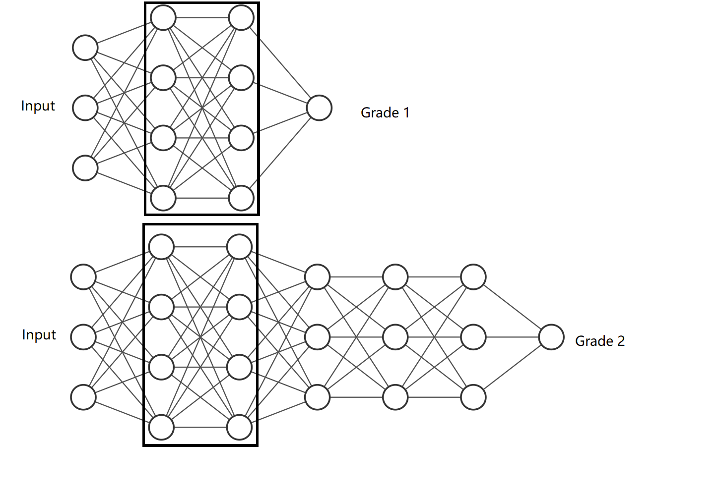
Figure 1: Multi-grade network with 2 grades

Next, we construct the neural network of grade 2, denoted by $u_{2}$, which is built on top of the neural network of grade 1, using a network $\mathcal{N}_{k_{2}}:=\mathcal{N}_{k_{2}}(\Theta_{2};\bullet)$ with parameters $\Theta_{2}=\{W_{j}^{2},b_{j}^{2}\}_{j=1}^{k_{2}}$. Specifically, we first remove the output layer of grade 1 and stack the network $\mathcal{N}_{k_{2}}$ on top of the last hidden layer of grade 1 to define the neural network of grade 2. That is,

$$u_{2}=u_{2}(\Theta_{1};\bullet):=\mathcal{N}_{k_{2}}(\Theta_{2};\bullet)\circ\mathcal{H}_{k_{1}-1}^{1*},$$

where “$\circ$” denotes the composition operator and $\mathcal{H}_{k_{1}-1}^{1*}$ is the network $\mathcal{N}_{k_{1}}^{*}$ without the output layer. We illustrate in Figure 1 the network structure of grade 1 and grade 2. From the construction process of a multi-grade network, it can be seen that traditional fully connected neural networks can be viewed as single-grade learning (SGL).

We learn the parameters of grade 2 by solving the minimization problem

(9) $$\min_{\Theta_{2}}Loss(u_{1}^{*}(\bullet)+u_{2}(\Theta_{2};\bullet))$$

to obtain the optimal parameters $\Theta_{2}^{*}:=\{W_{j}^{2*},b_{j}^{2*}\}_{j=1}^{k_{2}}$ and define

$$u_{2}^{*}:=u_{2}(\Theta_{2}^{*};\bullet)=\mathcal{N}_{k_{2}}(\Theta_{2}^{*};\bullet)\circ\mathcal{H}_{k_{1}-1}^{1*}.$$

Note that the parameters of $\mathcal{H}_{k_{1}-1}^{1*}$ are fixed during the minimization process (9). We can see from equation (9) that $u_{2}^{*}$ learns the residual of the solution $u_{1}^{*}$ of grade 1 to better approximate the solution of the PDE.

We can repeat this process to construct a neural network of $\ell+1$ grades. Assuming that for $1\leq i\leq\ell$, the neural networks $u_{i}$ of grade $i$ have been learned, we use a neural network $\mathcal{N}_{k_{\ell+1}}(\Theta_{\ell+1};\bullet)$ with parameters $\Theta_{\ell+1}=\{W_{j}^{\ell+1},b_{j}^{\ell+1}\}_{j=1}^{k_{\ell+1}}$ to define the neural network $u_{\ell+1}$ of grade $\ell+1$. That is,

(10) $$u_{\ell+1}(\Theta_{\ell+1};\mathbf{x}):=(\mathcal{N}_{k_{\ell+1}}(\Theta_{\ell+1};\bullet)\circ\mathcal{H}_{k_{\ell}-1}^{\ell*}\circ\dots\circ\mathcal{H}_{k_{2}-1}^{2*}\circ\mathcal{H}_{k_{1}-1}^{1*})(\mathbf{x}),$$

where $\mathcal{H}_{k_{i}-1}^{i*}$ denotes the neural network $\mathcal{N}_{k_{i}}^{*}:=\mathcal{N}_{k_{i}}(\Theta_{i}^{*};\bullet)$ without the output layer, with the learned parameters $\{W_{j}^{i*},b_{j}^{i*}\}_{j=1}^{k_{i}-1}$, $i=1,2,\dots,\ell$. The optimal parameters $\Theta_{\ell+1}^{*}=\{W_{j}^{\ell+1*},b_{j}^{\ell+1*}\}_{j=1}^{k_{\ell+1}}$ of grade $\ell+1$ is obtained by solving the minimization problem

(11) $$\min_{\Theta_{\ell+1}}Loss\left(\sum_{i=1}^{\ell}u_{i}^{*}(\bullet)+u_{\ell+1}(\Theta_{\ell+1};\bullet)\right).$$

It should be noted that the parameters of $\mathcal{H}_{k_{i}-1}^{i*}$, for $i=1,2,\dots,\ell$, are all fixed during the minimization process (11). We then let $u_{\ell+1}^{*}:=u_{\ell+1}(\Theta_{\ell+1}^{*};\bullet)$. Finally, by summing the approximations of all $\ell+1$ grades, we obtain the neural network

$$\bar{u}_{\ell+1}^{*}:=\sum_{i=1}^{\ell+1}u_{i}^{*}$$

and $\bar{u}_{\ell+1}^{*}$ serves as an approximate solution of the initial-boundary value problem (1)-(3). This approach allows us to solve several relatively small minimization problems, instead of one large problem. By using this MGDL method, we can better approximate the solution of the initial-boundary value problem of the PDE by learning the residual of the previous grades. This statement is justified by the following theoretical result.

Proposition 3.1.

Suppose that the neural network $\bar{u}_{\ell}^{*}:=\sum_{i=1}^{\ell}u_{i}^{*}$ with $\ell$ grades has been constructed. If $u_{\ell+1}(\Theta_{\ell+1};\mathbf{x})$ is defined as in (10) with trainable parameters $\Theta_{\ell+1}:=\{W_{j}^{\ell+1},b_{j}^{\ell+1}\}_{j=1}^{k_{\ell+1}}$, then there exists $\Theta_{\ell+1}^{*}$ such that

(12) $$Loss\left(\bar{u}_{\ell}^{*}(\bullet)+u_{\ell+1}(\Theta_{\ell+1}^{*};\bullet)\right)\leq Loss\left(\bar{u}_{\ell}^{*}(\bullet)\right).$$

Proof 3.2.

It can be verified directly from the definition (5) of deep neural networks that if the weight matrix and bias vector of the output layer are both set to 0, then the output of a fully connected neural network will be 0. In other words, the resulting deep neural network is a zero function. Following this observation, if the weight matrix and bias vector of the output layer are initialized as 0, that is, we choose

$$\Theta_{\ell+1}^{0}:=\{W^{\ell+1}_{j},b^{\ell+1}_{j}\}_{j=1}^{k_{\ell+1}},\ \ \mbox{with}\ \ W_{k_{\ell+1}}^{\ell+1}:=0\ \ \mbox{and}\ \ b_{k_{\ell+1}}^{\ell+1}:=0,$$

then we observe that

$$u_{\ell+1}(\Theta_{\ell+1}^{0};\mathbf{x})=0,\ \ \mbox{for all}\ \ \mathbf{x}\in\mathbb{R}^{s}.$$

Hence, the loss function will satisfy

(13) $$Loss\left(\bar{u}_{\ell}^{*}(\bullet)+u_{\ell+1}(\Theta_{\ell+1}^{0};\bullet)\right)=Loss\left(\bar{u}_{\ell}^{*}(\bullet)\right).$$

Let $\Theta_{\ell+1}^{*}$ be a solution of the minimization problem (11). Then, for the parameters $\Theta_{\ell+1}^{0}$ chosen as above, there holds that

$$Loss\left(\bar{u}_{\ell}^{*}(\bullet)+u_{\ell+1}(\Theta_{\ell+1}^{*};\bullet)\right) =\min_{\Theta_{\ell+1}}Loss\left(\bar{u}_{\ell}^{*}(\bullet)+u_{\ell+1}(\Theta_{\ell+1};\bullet)\right)$$

$$\leq Loss\left(\bar{u}_{\ell}^{*}(\bullet)+u_{\ell+1}(\Theta_{\ell+1}^{0};\bullet)\right)$$

$$=Loss\left(\bar{u}_{\ell}^{*}(\bullet)\right).$$

We have used equation (13) in the last equality of the above inequality. This yields inequality (12).

Proposition 3.1 shows that the value of the loss function is reduced as we move from grade $\ell$ to grade $\ell+1$.

It is important to point out that the traditional fully connected neural network can be viewed as single-grade learning, which has limitations in certain scenarios. Single-grade learning involves training a neural network with a fixed architecture and optimizing all the parameters at once. Although this approach can work well for simple problems, it can become challenging to train DNNs with many layers due to issues such as the vanishing gradient problem. Compared to single-grade learning, the MGDL approach has several advantages. First, it breaks down the learning process into multiple sub-problems, reducing the difficulty of learning a DNN. Second, it allows us to incorporate prior knowledge of the problem into the network architecture by building on top of previous grades. Third, it can alleviate overfitting by learning the network in a hierarchical manner, where each grade learns relevant features before moving on to the next.

4 A Two-Stage Multi-Grade Model and Implementation

This section is devoted to an introduction of a two-stage multi-grade deep learning (TS-MGDL) model for training a DNN solution for PDEs and its implementation.

The learning strategy described in the last section involves a grade-by-grade approach. As the number of grades increases, the residual oscillations that need to be learned become more pronounced. However, due to a relatively small number of layers in the neural network of each grade (typically less than 6 layers in our experiments to be presented later), the network may struggle to capture more complex patterns contained in the underlying residual oscillations. Moreover, the MGDL model may be trapped in a local minimizer and miss a global minimizer. Addressing these issues requires us to enlarge the search region for a minimizer. To this end, we unfreeze some layers of the network that have been trained in the last grade and some previous grades and retrain them all together to improve the accuracy of the resulting DNN solution. This process is referred to as the second stage of training. This process is analogous to human learning, where we periodically revisit and review material previously learned from several courses or even several grades in order to reinforce our understanding and identify gaps in our knowledge.

The second stage of training can be described below. Assume that after the first stage of training, we have constructed the neural network $\bar{u}_{L}^{*}:=\sum_{i=1}^{L}u_{i}^{*}$, with $L$ grades, which approximates the solution of the PDE. Note that the function $u_{L}^{*}$ has the following expression

$$u_{L}^{*}(\mathbf{x}):=(\mathcal{N}_{k_{L}}^{*}\circ\mathcal{H}_{k_{L}-1}^{L-1*}\circ\dots\circ\mathcal{H}_{k_{2}-1}^{2*}\circ\mathcal{H}_{k_{1}-1}^{1*})(\mathbf{x}),$$

where $\mathcal{N}_{k_{L}}^{*}$ is trained in grade $L$ with learned parameters $\Theta_{L}^{*}$. We unfreeze the last $k$ layers of $u_{L}^{*}$ as the new trainable layers, with $k>k_{L}$. We denote by

$$\Theta_{L,k}:=\{{W}_{j}^{L,k},{b}_{j}^{L,k}\}_{j=1}^{k}$$

the parameters of the $k$ trainable layers in the second stage of training. Note that $\Theta_{L,k}$ includes not only the parameters of $\mathcal{N}_{k_{L}}$ intended to be trained in grade $L$, but also some layers of the networks learned in previous grades. We use the notation $\widetilde{u}_{L}:=\widetilde{u}_{L}(\Theta_{L,k};\bullet)$ to denote the neural network obtained from $u_{L}^{*}$ by unfreezing its last $k$ layers and solve the minimization problem

(14) $$\min_{\Theta_{L,k}}Loss(\bar{u}_{L-1}^{*}(\bullet)+\widetilde{u}_{L}(\Theta_{L,k};\bullet)).$$

We solve the minimization problem (14) using the parameters of the $k$ layers of $u_{L}^{*}$ as an initial guess and obtain the new parameters $\Theta_{L,k}^{*}$. We then define the function $\widetilde{u}_{L}^{*}:=\widetilde{u}_{L}(\Theta_{L,k}^{*};\bullet)$. As such, the second stage generates the approximate solution of the PDE, given by

$$u_{appr}:=\bar{u}_{L-1}^{*}+\widetilde{u}_{L}^{*}.$$

We summarize the TS-MGDL algorithm described above for solving nonlinear PDEs in Algorithm 1.

Algorithm 1 Two-stage multi-grade deep learning (TS-MGDL) for solving nonlinear PDE

0:  Number of grades $L$ and number of layers $k_{i}$ for each grade $i=1,\dots,L$. Nonlinear differential operator $\mathcal{F}$, initial condition $\mathcal{I}$, and boundary condition $\mathcal{B}$.

0:  Approximate solution of the PDE. Stage 1: Learn the network grade by grade.

1:  Initialize: $\mathcal{N}_{k_{1}}$ with parameters $\Theta_{1}=\{W_{i}^{1},b_{i}^{1}\}_{i=1}^{k_{1}}$.

2:  Obtain $u_{1}^{*}(\mathbf{x})=\mathcal{N}_{k_{1}}^{*}$ by solving minimization problem (8).

3:  Initialize $\ell=1$.

4:  while $\ell\leq L$ do

5:     Initialize $\mathcal{N}_{k_{\ell+1}}$ with parameters $\Theta_{\ell+1}=\{W_{j}^{\ell+1},b_{j}^{\ell+1}\}_{j=1}^{k_{\ell+1}}$.

6:     Set grade $\ell+1$ network $u_{\ell+1}(\mathbf{x})=(\mathcal{N}_{k_{\ell+1}}\circ\mathcal{H}_{k_{\ell}-1}^{\ell*}\circ\dots\circ\mathcal{H}_{k_{2}-1}^{2*}\circ\mathcal{H}_{k_{1}-1}^{1*})(\mathbf{x})$.

7:     Obtain $u_{\ell+1}^{*}$ by solving the minimization problem (11).

8:     $\ell\leftarrow\ell+1$.

9:  end whileStage 2: Learn the network by layer unfreezing.

10:  Let $\widetilde{u}_{L}=u_{L}^{*}$ and set the $k$ last layers trainable in the network $\widetilde{u}_{L}$.

11:  Obtain $\widetilde{u}_{L}^{*}$ by solving the minimization problem (14) with the initial guess $u_{L}^{*}$.

12:  Let $u_{appr}=\bar{u}_{L-1}^{*}+\widetilde{u}_{L}^{*}$.

13:  Output: Approximate solution $u_{appr}$ of the PDE.

Recall that we have showed in Proposition 3.1 that the value of the loss function is reduced as we move from grade $\ell$ to grade $\ell+1$ in the first stage. Our next proposition shows that the second stage of the TS-MGDL method can further reduce the value of the loss function.

Proposition 4.1.

If the neural network $\bar{u}_{L}^{*}:=\sum_{i=1}^{L}u_{i}^{*}$ with $L$ grades has been constructed and $k>k_{L}$, then there exists $\Theta_{L,k}^{*}:=\{W_{j}^{L,k*},b_{j}^{L,k*}\}_{j=1}^{k}$ such that

(15) $$Loss\left(\bar{u}_{L-1}^{*}(\bullet)+\widetilde{u}_{L}(\Theta_{L.k}^{*};\bullet)\right)\leq Loss\left(\bar{u}_{L}^{*}(\bullet)\right).$$

Proof 4.2.

Without loss of generality, we assume that the parameters of the last $k$ layers of $u_{L}^{*}$ are unfrozen and retrained. We denote by

(16) $$\Theta_{L,k}^{\prime}:=\{W_{j}^{L,k},b_{j}^{L,k}\}_{j=1}^{k}$$

the parameters of the last $k$ layers of $u_{L}^{*}$, which have been trained in the first stage of the MGDL method of $L$ grades. We then have that

$$\widetilde{u}_{L}(\Theta_{L,k}^{\prime};\bullet)=u_{L}^{*}(\bullet).$$

This together with the relation $\bar{u}_{L}^{*}=\bar{u}_{L-1}^{*}+u_{L}^{*}$ yields that

(17) $$Loss\left(\bar{u}_{L-1}^{*}(\bullet)+\widetilde{u}_{L}(\Theta_{L,k}^{\prime};\bullet)\right)=Loss\left(\bar{u}_{L}^{*}(\bullet)\right).$$

Let $\Theta_{L,k}^{*}$ be a solution of the minimization problem (14). Then, for the parameters $\Theta_{L,k}^{\prime}$ chosen as (16), by employing equation (17), we obtain that

$$Loss\left(\bar{u}_{L-1}^{*}(\bullet)+\widetilde{u}_{L}(\Theta_{L,k}^{*};\bullet)\right) =\min_{\Theta_{L,k}}Loss\left(\bar{u}_{L-1}^{*}(\bullet)+\widetilde{u}_{L}(\Theta_{L,k};\bullet)\right)$$

$$\leq Loss\left(\bar{u}_{L-1}^{*}(\bullet)+\widetilde{u}_{L}(\Theta_{L,k}^{\prime};\bullet)\right)$$

$$=Loss\left(\bar{u}_{L}^{*}(\bullet)\right),$$

which leads to inequality (15).

Proposition 4.1 confirms that the value of the loss function is reduced as the TS- MGDL method moves from stage 1 to stage 2. Propositions 3.1 and 4.1 together reveal that every grade and stage can reduce the value of the loss function. This fact will be further validated by numerical experiments in the next section.

Discussion of several crucial implementation issues is in order. The number $k$ of trainable layers in the TS-MGDL algorithm has a significant impact on performance. Having too few trainable layers can restrict the learning capacity of the network. On the other hand, having too many trainable layers can lead to excessive computational costs and result in unstable or non-convergent training. To strike a balance between expressive power and convergence, in our experiments to be presented later, we choose $k:=8$ layers that are closest to the output of the neural network $u_{L}^{*}$ as the trainable layers. This allows the model to retain sufficient expressive power while ensuring stable and efficient training.

Setting an appropriate learning rate is crucial to solving the resulting optimization problems. The MGDL method enables the use of different learning rates for different grades, providing greater flexibility in optimizing the network. The key advantage of using different learning rates for different grades is that it allows the network to learn the relevant features more quickly and accurately. In our experiments, we set a higher learning rate for earlier grades so that the network can learn the basic (large scale) features quickly and move on to learning more complex (small scale) features. This can speed up the training process and improve the overall accuracy of the network. While using a lower learning rate for later grades helps fine-tune the learned representations and improve the accuracy of the network. In the second stage of training, using a low learning rate enables the network to carefully adjust these representations to better fit the training data, leading to improved accuracy.

In implementing the TS-MGDL algorithm, the choice of the number of epochs for each grade has a significant impact on the final result. If the number of epochs is too big in earlier grades, it is likely to get trapped in unwanted local minima, which can make it difficult to optimize the subsequent grades. In the training process of the first stage, as the grade increases, the training difficulty gradually intensifies, and the number of epochs should increase accordingly. Since gradient descent typically exhibits a faster decrease in loss at the beginning of iterations, we can leverage this by setting a small number of epochs for the grades in the first stage to capture the rapidly descending phase. On the other hand, a larger number of epochs is recommended in the second stage to achieve an enhanced numerical approximation.

The TS-MGDL method seamlessly integrates the ideas of greedy learning, residual learning, pre-training, and fine-tuning. There are several benefits of this method in solving PDEs, which we summarize below.

• Improved Global Optima: The two-stage approach helps in finding better global optima. In the first stage, the TS-MGDL method incrementally increases the network depth, allowing efficient local optimization and finding a good initial solution. The second stage involves unfreezing and additional training, which explores in a broader parameter space and refines the model. By considering a wider range of possible solutions, the method increases the chance of finding better global optima, leading to improved accuracy.

• Accelerated Convergence: The TS-MGDL method accelerates the convergence of the optimization process. Training on relatively shallow networks in the first stage mitigates gradient vanishing and exploding issues, allowing for stable and effective learning. By gradually increasing the complexity and capacity of the network, the method facilitates the convergence of deeper networks in the second stage, leading to faster convergence and efficient optimization.

• Implicit Regularization: The TS-MGDL method incorporates implicit regularization. In the first stage, the algorithm gradually increases the complexity of the network to avoid premature attempts to learn intricate relationships, helping prevent overfitting. In the second stage, only the unfrozen layers are allowed to adapt and fine-tune their parameters. This approach grants the model to refine its learned representations in a controlled manner, balancing the risk of overfitting with the need for improved prediction accuracy.

• Improved Accuracy: The multi-grade algorithm enhances accuracy via a combination of residual learning and fine-tuning. In the first stage, the network is trained incrementally, one grade at a time, progressively incorporating increasingly detailed information to improve accuracy. By capturing residual information, the algorithm captures intricate details and improves accuracy. The progressive training approach establishes a solid foundation, while selective retraining in the second stage refines predictions and further improves accuracy.

To evaluate the effectiveness of the proposed TS-MGDL method, we conducted numerical experiments on the 1D, 2D, and 3D Burgers equations. Numerical results demonstrate that the MGDL approach can achieve higher accuracy and faster convergence compared to the single-grade learning method. We will present our numerical findings in the next section.

5 Applications to the Burgers Equation and Numerical Experiments

In this section, we apply the proposed TS-MGDL method to numerical solutions of the 1D, 2D, and 3D Burgers equations and present numerical results. In particular, we validate the theoretical results of Propositions 3.1 and 4.1 and compare the numerical performance of the TS-MGDL method with that of the traditional single-grade learning method.

All the experiments presented in this section were carried out on a 64-bit Linux server equipped with 125GB of physical memory and an Intel(R) Xeon(R) Silver 4116 CPU with a clock speed of 2.10GHz. The Nvidia Tesla V100 graphics card is utilized to accelerate training. Both the multi-grade learning method and single-grade method were implemented using the DeepXDE [20] and Tensorflow 2.8 frameworks.

In the experiments that follow, the activation function for all the neural networks is $\tanh$. In the experiments, we use the relative $L_{2}$ error to measure the error between the approximate solution and the true solution, in order to compare the accuracy of the TS-MGDL method and the SGL method. The relative $L_{2}$ error is defined by

$$\frac{\|u-u^{\ast}\|_{2}}{\|u\|_{2}}=\frac{\sqrt{\sum_{i=1}^{N}(u(\mathbf{x_{i}})-u^{\ast}(\mathbf{x_{i}}))^{2}}}{\sqrt{\sum_{i=1}^{N}u(\mathbf{x_{i}})^{2}}},$$

where $u^{\ast}$ is the approximate solution, $u$ is the true solution, and $\mathbf{x_{i}}$ are points in the test set.

5.1 The 1D Burgers equation

In this example, we consider the 1D Burgers equation, which takes the form

(18) $$u_{t}(t,x)+u(t,x)u_{x}(t,x)-\frac{0.01}{\pi}u_{xx}(t,x)=0,\quad t\in(0,1],\ x\in(-1,1),$$

where $u(t,x)$ represents the velocity of the fluid at time $t$ and position $x$, $u_{x}(t,x)$ and $u_{xx}(t,x)$ denote its first and second spatial derivatives, respectively. The initial condition for this equation is given by

(19) $$u(0,x)=-\sin(\pi x),$$

which represents a sinusoidal velocity profile at time $t=0$. The boundary conditions are given by

(20) $$u(t,-1)=u(t,1)=0,$$

which specify that the velocity of the fluid is zero on the boundaries of the domain, $x=-1$ and $x=1$, for all times $t$.

According to [3], the analytic solution of the initial-boundary value problem of the 1D Burgers equation takes the form

$$u(t,x)=-\frac{\int_{-\infty}^{+\infty}\sin\pi(x-\eta)h(x-\eta)\exp\left(-\eta^{2}/4\nu t\right)\mathrm{d}\eta}{\int_{-\infty}^{+\infty}h(x-\eta)\exp\left(-\eta^{2}/4\nu t\right)\mathrm{d}\eta},\ \ t\in[0,1],\ x\in[-1,1],$$

where $\nu:=0.01/\pi$ and $h(y):=\exp(-\cos\pi y/2\pi\nu)$. The analytic solution, shown in Figure 2, which exhibits a big change at $x=1$ when $t>0.4$, will be used for comparison of the TS-MGDL and the SGL methods.

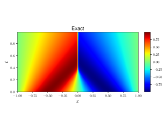
Figure 2: Exact solution of 1D Burgers’ equation.

We employed the Hammersley sampling method to randomly generate training sample points. Along the boundaries, a total of $N_{b}:=80$ random points were generated. Furthermore, $N_{0}:=120$ random points were generated based on the initial conditions. In the interior region $(0,1]\times(-1,1)$, there are $N_{f}:=10,000$ random points generated. The test set consists of evenly spaced grid points obtained by dividing the spatiotemporal region $[0,1]\times[-1,1]$. The total number of test points is $100\times 256$.

Table 1 presents three different network structures (SGL-1, SGL-2, and SGL-3) of the SGL method for solving the 1D Burgers equation. They all consist of 2 input neurons and 1 output neuron. Each of the network structures is represented by a list of integers, which indicate the number of neurons in the corresponding layers of the network.

Table 2 displays the network structures (Grade 1, Grade 2, and Grade 3) of the TS-MGDL model for solving the 1D Burgers equation. Each neural network has 2 input neurons and 1 output neuron. To facilitate comparison, the network structures of SGL-1 and Grade 1 of the TS-MGDL model are set to be the same. Likewise, the network structures of SGL-2 and Grade 2 of the TS-MGDL model are set to be the same, and the network structures of SGL-3 and Grade 3 of the TS-MGDL model are also set to be the same. This ensures that any differences in performance between these methods can be attributed to the different learning strategies employed, rather than differences in network architecture. An asterisk (*) next to a number in the list indicates that the corresponding weight parameters are fixed to be those trained in the previous grades during training in the present grade of the first stage. Only those layers without an asterisk will be trained in the current grade. In the second stage of training, the last 8 hidden layers of the Grade 3 network will be unfrozen, which are located near the output. This means that the weights of these layers will be allowed to change during training.

Methods	Network structure
SGL-1	[2, 128, 128, 128, 128, 128, 128, 1 ]
SGL-2	[2, 128, 128, 128, 128, 128, 128, 256, 256, 1]
SGL-3	[2, 128, 128, 128, 128, 128, 128, 256, 256, 256, 256, 256, 128, 1]

Table 1: Network structure of single-grade learning for the 1D Burgers equation.

Grade	Network structure
1	[2, 128, 128, 128, 128, 128, 128, 1 ]
2	[2, 128*, 128*, 128*, 128*, 128*, 128*, 256, 256, 1]
3	[2, 128*, 128*, 128*, 128*, 128*, 128*, 256*, 256*, 256, 256, 256, 128, 1]

Table 2: Network structure of multi-grade learning for the 1D Burgers equation.

Table 3 presents the numerical results of the TS-MGDL model for solving the 1D Burgers equation. The training process is divided into two stages. In the first stage of training, we use a learning rate of 1e-3 for Grade 1. As we move to Grades 2 and 3, the learning rate is reduced while the number of epochs is increased to 100,000. This helps balance the trade-off between learning complex representations and preventing overfitting. In the second stage of training, we use a learning rate of 3e-4 and 300,000 epochs to fine-tune the network’s learned representations.

As we can see from Table 3, the relative $L_{2}$ error decreases as we move from lower to higher grades within the first stage of training. Specifically, in Stage 1, Grade 1, we obtain a relative $L_{2}$ error of 7.45e-04, which decreases to 3.30e-04 in Grade 2 and further to 1.15e-04 in Grade 3. This demonstrates that increasing the number of grades can improve performance. In Stage 2, the relative $L_{2}$ error is further reduced to 9.65e-06 through fine-tuning of the Grade 3 network.

Stage & grade	Learning rate	Decay rate	Epochs	Relative $L_{2}$ error
Stage 1, Grade 1	1e-3	1e-4	50,000	7.45e-04
Stage 1, Grade 2	3e-4	1e-4	100,000	3.30e-04
Stage 1, Grade 3	2e-4	1e-4	100,000	1.15e-04
Stage 2	3e-4	1e-4	300,000	9.65e-06

Table 3: Numerical results of the TS-MGDL method for the 1D Burgers equation.

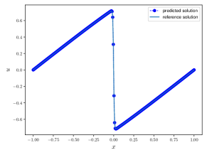
(a) $u_{1}^{*}$ generated from Grade 1

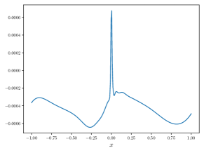
(b) $u_{2}^{*}$ generated from Grade 2

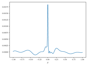
(c) $u_{3}^{*}$ generated from Grade 3

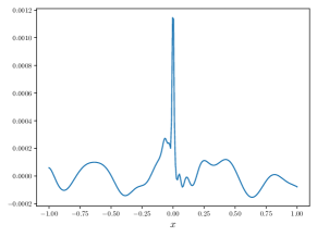
(d) $\widetilde{u}_{3}^{*}$ generated from Stage 2

Figure 3: Numerical results of TS-MGDL for the 1D Burgers equation at $t=0.99$.

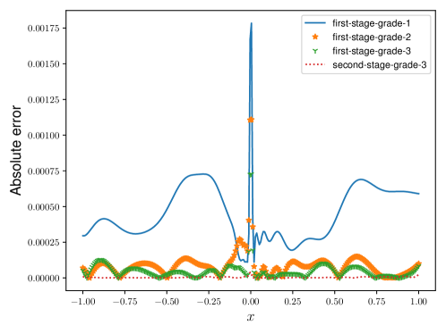
Figure 4: Absolute errors of TS-MGDL for the 1D Burgers equation at $t=0.99$.

Table 4 compares the performance of single-grade learning models (SGL-1, SGL-2, and SGL-3) and the TS-MGDL model for solving the 1D Burgers equation. The hyperparameters used for training the SGL neural networks include a learning rate of 1e-3, a decay rate of 1e-4, and 550,000 epochs for each model. The relative $L_{2}$ error for SGL-1 is 5.75e-04, for SGL-2 is 3.02e-04, and for SGL-3 is 2.53e-04. In comparing the numerical results of the TS-MGDL and SGL methods, we can see that TS-MGDL achieves lower relative $L_{2}$ errors than SGL. The TS-MGDL method achieves a relative $L_{2}$ error of 9.65e-06, which is significantly lower than the lowest error achieved by any of the SGL methods, which is 2.53e-04. Moreover, Grades 2 and 3 of Stage 1 generate approximate solutions having accuracy comparable to those generated by SGL-2 and SGL-3, but require significantly less epochs. All these facts suggest that TS-MGDL is more effective than the SGL method for problems with complex solutions, as it approximates the solution of the PDE by gradually increasing the complexity of the neural network.

Methods	Learning rate	Decay rate	Epochs	Relative $L_{2}$ error
SGL-1	1e-3	1e-4	550,000	5.75e-04
SGL-2	1e-3	1e-4	550,000	3.02e-04
SGL-3	1e-3	1e-4	550,000	2.53e-04
TS-MGDL	–	–	550,000	9.65e-06

Table 4: Numerical results for the 1D Burgers equation.

Figure 3 illustrates the results of TS-MGDL at time $t=0.99$. Figures 3a, 3b, and 3c display the solution components $u_{1}^{*}$, $u_{2}^{*}$ and $u_{3}^{*}$ achieved at Grade 1, Grade 2, and Grade 3, respectively. Figure 3d displays the solution component $\widetilde{u}_{3}^{*}$ generated in stage 2, showing that $\widetilde{u}_{3}^{*}$ contains richer information than $u_{3}^{*}$ does. Figure 4 provides a comparison of the absolute errors between the predicted and true solutions at $t=0.99$, for Grades 1,2,3 and Stage 2. The results indicate that the TS-MGDL method approximates the solution well, with the error gradually decreasing from grade 1 to grade 3. After the training in the second stage, the error in the solution becomes significantly smaller than that of the first stage, indicating the effectiveness of the TS-MGDL method in improving the accuracy of the solution.

Figure 5 shows the training loss for SGL-1, SGL-2, SGL-3, and TS-MGDL. It can be observed that the SGL methods exhibit significant oscillations in the loss curve during the later stages of training, leading to slow convergence and a delayed reduction in loss. The loss curve for the TS-MGDL method exhibits a smooth descent without pronounced oscillations, indicating stable convergence. Moreover, the TS-MGDL method demonstrates a faster rate of loss reduction. In particular, Figure (5d) confirms the theoretical results stated in both Propositions 3.1 and 4.1 for the 1D Burgers equation. These findings highlight the superiority of the TS-MGDL approach in terms of both accuracy and efficiency when approximating solutions for the 1D Burgers equation.

The figures presented in Figure 6 depict the predicted solutions and absolute errors for SGL-1, SGL-2, SGL-3, and TS-MGDL, for solving the 1D Burgers equation. Compared to the SGL methods, it is evident that the TS-MGDL method achieves a significantly smaller absolute error.

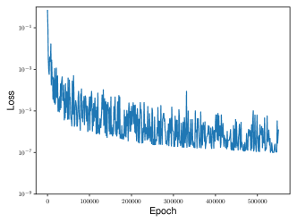
(a) SGL-1

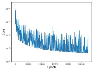
(b) SGL-2

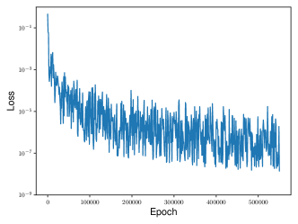
(c) SGL-3

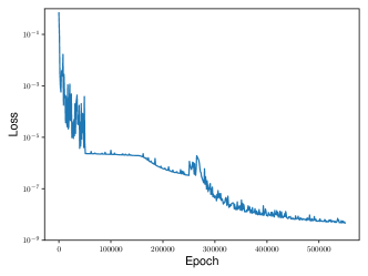
(d) TS-MGDL

Figure 5: Training loss for SGL-1, SGL-2, SGL-3, and TS-MGDL for the 1D Burgers equation.

(a) Predicted solution of SGL-1

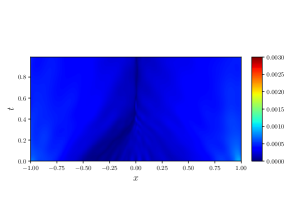
(b) Absolute error of SGL-1

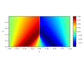
(c) Predicted solution of SGL-2

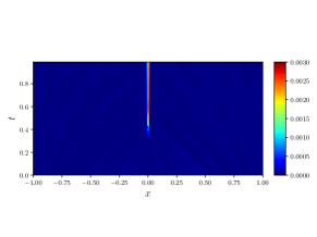
(d) Absolute error of SGL-2

(e) Predicted solution of SGL-3

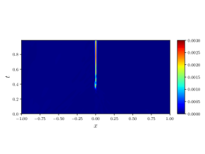
(f) Absolute error of SGL-3

(g) Predicted solution of TS-MGDL

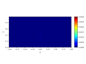
(h) Absolute error of TS-MGDL

Figure 6: Comparison of SGL1, SGL2, SGL3 with TS-MGDL for the 1D Burgers equation.

5.2 The 2D Burgers equation

In this example, we consider the 2D Burgers equation over a square domain $\Omega:=[0,1]^{2}$ in the form

(21) $$\begin{gathered}\frac{{\partial}u}{\partial t}+u\frac{{\partial}u}{\partial x}+u\frac{{\partial}u}{\partial y}=\nu\left(\frac{{\partial}^{2}u}{\partial x^{2}}+\frac{{\partial}^{2}u}{\partial y^{2}}\right),\ \ (x,y)\in\Omega,\ \ t\in(0,1],\end{gathered}$$

where $u$ represents the velocity, $\nu:=\frac{1}{Re}$ is the kinematic viscosity coefficient, and $Re$ is the Reynolds number. In this example, we set Reynolds number $Re:=100$. The initial condition is given by:

(22) $$u(0,x,y)=\frac{1}{1+e^{Re(x+y)}},\ \ (x,y)\in\Omega.$$

The boundary conditions are given by:

(23) $$u(t,0,y)=\frac{1}{1+e^{\frac{Re(y-t)}{2}}},\ \ u(t,1,y) =\frac{1}{1+e^{\frac{Re(1+y-t)}{2}}},y\in[0,1],\ \ t>0,$$

$$u(t,x,0)=\frac{1}{1+e^{\frac{Re(x-t)}{2}}},\ \ u(t,x,1) =\frac{1}{1+e^{\frac{Re(1+x-t)}{2}}},x\in[0,1],\ \ t>0.$$

The exact solution of the initial boundary value problem takes the form:

(24) $$u(x,y,t)=\frac{1}{1+e^{\frac{Re(x+y-t)}{2}}},\quad(x,y)\in\Omega,\ \ t\geq 0.$$

We show in Figure 7 the exact solution $u(x,y,1)$ at $t=1$, which exhibits a significant increase across the line $x+y=1$.

In this example, the training point set is randomly generated using the Hammersley sampling method and consists of three components: $N_{f}:=20,000$ points located within the interior region $(0,1]\times(0,1)^{2}$, $N_{0}:=1,000$ points satisfying the initial condition (22), and $N_{b}:=2,000$ points satisfying the boundary conditions (23). The testing point set consists of $15\times 15$ equally spaced grid points in the spatial domain $[0,1]^{2}$ and a total of 224 equally spaced sampling points in the time interval [0, 1]. Therefore, there are a total of $224\times 15\times 15=50,400$ points in the testing set.

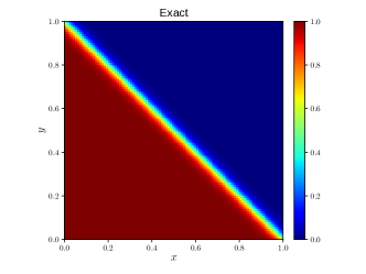
Figure 7: Exact solution of the 2D Burgers equation at $t=1$.

Table 5 provides an overview of the network structures used in the single-grade learning (SGL) methods to solve the 2D Burgers equation. It shows that as the method number increases, the network structures become progressively deeper, with SGL-3 having the deepest network structure.

Table 6 presents the network structures used in the TS-MGDL method. Notably, Grades 1, 2, and 3 share the identical network structure with SGL-1, SGL-2, and SGL-3, respectively. In Table 6, the asterisk (*) notation indicates that the layer’s parameters were frozen during the first stage of training. It is noteworthy that during the second stage of training, the last eight hidden layers of the Grade 3 neural network are unfrozen and undergo retraining to further refine the model.

Methods	Network structure
SGL-1	[3, 1024, 1024, 1]
SGL-2	[3, 1024, 1024, 1024, 512, 512, 1]
SGL-3	[3, 1024, 1024, 1024, 512, 512, 512, 512, 256, 256, 1]

Table 5: Network structure of single-grade learning for the 2D Burgers equation.

Grade	Network structure
1	[3, 1024, 1024, 1]
2	[3, 1024*, 1024*, 1024, 512, 512, 1]
3	[3, 1024*, 1024*, 1024*, 512*, 512*, 512, 512, 256, 256, 1]

Table 6: Network structure of multi-grade learning for the 2D Burgers equation.

Table 7 presents the numerical results of TS-MGDL methods. It shows that the relative $L_{2}$ error decreases as the grade number increases in the first stage, and the second stage further improves the accuracy. The relative $L_{2}$ error of the TS-MGDL method is 4.75e-05.

Stage & grade	Learning rate	Decay rate	Epochs	Relative $L_{2}$ error
Stage 1, Grade 1	1e-3	1e-4	10,000	1.63e-03
Stage 1, Grade 2	3e-4	1e-4	20,000	1.77e-04
Stage 1, Grade 3	3e-4	1e-4	40,000	1.28e-04
Stage 2	3e-4	7e-5	80,000	4.75e-05

Table 7: Numerical results of TS-MGDL for the 2D Burgers equation.

Table 8 compares the numerical results of TS-MGDL with those of SGL methods. The hyperparameters used for training the SGL neural networks include a learning rate of 1e-3, a decay rate of 1e-4, and 150,000 epochs for each method. Table 8 shows that SGL-2 achieves the relative $L_{2}$ error 1.39e-04, which is the smallest relative $L_{2}$ error among the SGL methods. It shows that for single-grade learning, it may become harder to optimize as the network goes deeper, which can lead to a decrease in accuracy. The TS-MGDL method achieves a significantly smaller relative $L_{2}$ error than any of the SGL methods, demonstrating the effectiveness of multi-grade learning in solving the 2D Burgers equation.

Methods	Learning rate	Decay rate	Epochs	Relative $L_{2}$ error
SGL-1	1e-3	1e-4	150,000	2.00e-04
SGL-2	1e-3	1e-4	150,000	1.39e-04
SGL-3	1e-3	1e-4	150,000	1.46e-03
TS-MGDL	–	–	150,000	4.75e-05

Table 8: Numerical results for the 2D Burgers equation.

Figure 8 shows the training loss of the SGL-1, SGL-2, SGL-3, and TS-MGDL methods for solving the 2D Burgers equation. The figures in Figure 9 depict the approximation solutions and absolute errors of four methods. From the results, it can be observed that the TS-MGDL method exhibits smaller errors compared to the single-grade learning (SGL) methods. The loss curves of the SGL methods show significant oscillations and slow convergence. On the other hand, the loss curve of the TS-MGDL method demonstrates a smoother and faster decrease in loss. Figure 8d confirms the theoretical results stated in Propositions 3.1 and 4.1 for the 2D equation. These findings suggest that the TS-MGDL method outperforms the SGL methods in terms of accuracy and convergence speed.

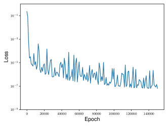
(a) SGL-1

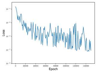
(b) SGL-2

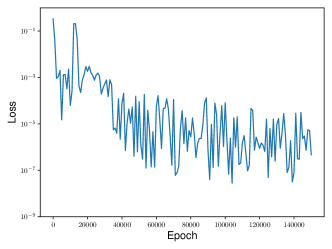
(c) SGL-3

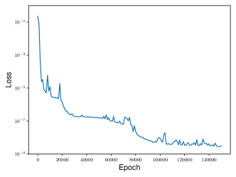
(d) TS-MGDL

Figure 8: Training loss for SGL-1, SGL-2, SGL-3, and TS-MGDL for the 2D Burgers equation.

(a) Predicted solution of SGL-1

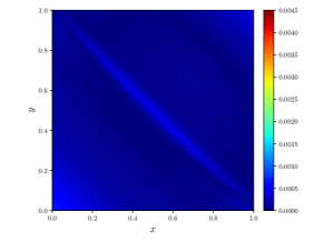
(b) Absolute error of SGL-1

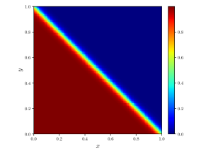
(c) Predicted solution of SGL-2

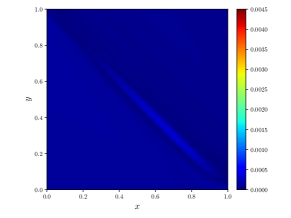
(d) Absolute error of SGL-2

(e) Predicted solution of SGL-3

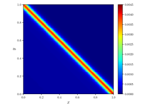
(f) Absolute error of SGL-3

(g) Predicted solution of TS-MGDL

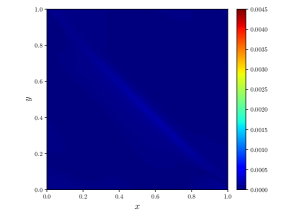
(h) Absolute error of TS-MGDL

Figure 9: Comparision between SGL methods and TS-MGDL method for the 2D Burgers equation at $t=1$.

5.3 The 3D Burgers equation

In this example, we consider solving the initial boundary value problem of the 3D Burgers equation defined in $\Omega:=[0,1]^{3}$, which can be expressed as follows:

(25) $$u_{t}+uu_{x}+uu_{y}+uu_{z}=\nu\left(u_{xx}+u_{yy}+u_{zz}\right)+f,\ \ (t,x,y,z)\in(0,1]\times\Omega,$$

$$u(t,x,y,z)=g(t,x,y,z),\quad t\in(0,1],(x,y,z)\in\partial\Omega,$$

$$u(0,x,y,z)=h(x,y,z),\quad(x,y,z)\in\Omega,$$

where $\nu:=\frac{1}{Re}>0$ represents the viscosity coefficient, and $Re$ is the Reynolds number. The exact solution of the equation (25) is given by:

(26) $$u(t,x,y,z)=\frac{1}{1+\mathrm{e}^{\frac{x+y+z-t}{2\nu}}}.$$

In the experiment, the function values of $f$, $g$, and $h$ in equation (25) were computed according to the exact solution (26). In this example, the Reynolds number $Re$ is set to 1. The exact solution of the 3D Burgers equation at $t=1$ is shown in Figure 10.

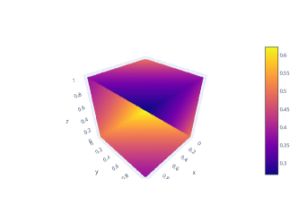
Figure 10: Exact solution of the 3D Burgers equation at $t=1$.

The training point set is generated randomly using the Hammersley sampling method. It is structured as follows: $N_{f}:=10,000$ points are located within the interior region $(0,1]\times(0,1)^{3}$, $N_{b}:=2,000$ points satisfy the boundary condition, and $N_{0}:=1,000$ points meet the initial condition. As for the testing point set, it consists of a uniform grid comprising $7^{3}$ points in the spatial domain $[0,1]^{3}$, along with 265 equally spaced sampling points in the time interval [0, 1]. This combination results in a total of $265\times 7^{3}=90,895$ points in the testing set.

Table 9 illustrates the network structures employed by the SGL methods. As the method number increases, the network structures of the SGL methods become progressively deeper. Table 10 presents the network structures of the TS-MGDL method. In this particular example, the TS-MGDL method consists of three grades. The network structure of Grade 1, 2, and 3 is identical to that of SGL-1, SGL-2, and SGL-3, respectively. In Table 10, the asterisk (*) notation indicates that the parameters of the corresponding layer were kept fixed during the first stage of training. During the second stage of training, the last eight hidden layers of the Grade 3 neural network are unfrozen and retrained.

Methods	Network structure
SGL-1	[4, 256, 256, 256, 256, 1]
SGL-2	[4, 256, 256, 256, 256, 512, 512, 256, 1]
SGL-3	[4, 256, 256, 256, 256, 512, 512, 256, 512, 512, 512, 256, 1]

Table 9: Network structure of single-grade learning for the 3D Burgers equation.

Grade	Network structure
1	[4, 256, 256, 256, 256, 1]
2	[4, 256*, 256*, 256*, 256*, 512, 512, 256, 1]
3	[4, 256*, 256*, 256*, 256*, 512*, 512*, 256*, 512, 512, 512, 256, 1]

Table 10: Network structure of multi-grade learning for the 3D Burgers equation.

Table 11 shows the numerical results of the TS-MGDL method. In Stage 1, the method progressively refines its approximate solution of the 3D Burgers equation through different grades, resulting in decreasing relative $L_{2}$ errors. In Stage 2, the TS-MGDL method further enhances its accuracy, attaining an impressive relative $L_{2}$ error of 8.90e-05. The TS-MGDL method’s ability to refine and adapt its learning through multiple stages and grades enables it to capture intricate dynamics, thereby resulting in enhanced accuracy when solving the 3D Burgers equation.

Stage & grade	Learning rate	Decay rate	Epochs	Relative $L_{2}$ error
Stage 1, Grade 1	4e-4	1e-4	3,000	2.95e-03
Stage 1, Grade 2	4e-4	1e-4	6,000	7.39e-04
Stage 1, Grade 3	4e-4	1e-4	6,000	3.92e-04
Stage 2	5e-4	1e-4	25,000	8.90e-05

Table 11: Numerical results of multi-grade learning for the 3D Burgers equation.

Table 12 presents a comparison of the numerical results obtained from SGL-1, SGL-2, SGL-3, and TS-MGDL methods for solving the 3D Burgers equation. The results demonstrate that the TS-MGDL method outperforms the SGL methods in terms of achieving a smaller relative $L_{2}$ error within the same number of training epochs. For SGL-1, SGL-2, and SGL-3, the learning rate is set to 4e-4, the decay rate is 1e-4, and the training is conducted for 40,000 epochs. Among the SGL methods, SGL-2 achieves the highest accuracy with a relative $L_{2}$ error of 1.77e-04. However, the TS-MGDL method exhibits the best overall performance, surpassing all SGL methods, with a relative $L_{2}$ error of 8.90e-05.

Methods	Learning rate	Decay rate	Epochs	Relative $L_{2}$ error
SGL-1	4e-4	1e-4	40,000	1.06e-03
SGL-2	4e-4	1e-4	40,000	1.77e-04
SGL-3	4e-4	1e-4	40,000	3.35e-04
TS-MGDL	–	–	40,000	8.90e-05

Table 12: Numerical results for the 3D Burgers equation.

Figure 11 illustrates the training loss curves for the SGL-1, SGL-2, SGL-3, and TS-MGDL methods. We can see that the TS-MGDL method demonstrates a significantly faster rate of decline in training loss compared to the SGL methods. In fact, the TS-MGDL method achieves the lowest overall loss among the evaluated methods. Moreover, the loss curve for TS-MGDL exhibits minimal oscillations, indicating a stable convergence process.

Figure 12 shows the computational results and error plots of the SGL-1, SGL-2, SGL-3, and TS-MGDL methods for the 3D Burgers equation at $t=1$. As can be seen in Figure 12, the TS-MGDL method provides a better approximation to the true solution, with smaller absolute errors. Once again, the theoretical results stated in Propositions 3.1 and 4.1 are verified by Figure 11d.

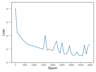
(a) SGL-1

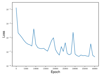
(b) SGL-2

(c) SGL-3

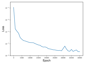
(d) TS-MGDL

Figure 11: Training loss for SGL-1, SGL-2, SGL-3, and TS-MGDL for the 3D Burgers equation.

(a) Predicted solution of SGL-1

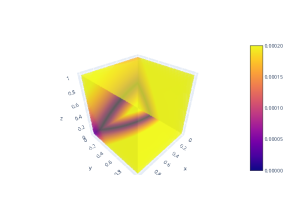
(b) Absolute error of SGL-1

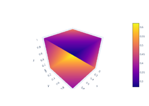
(c) Predicted solution of SGL-2

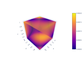
(d) Absolute error of SGL-2

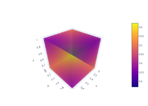
(e) Predicted solution of SGL-3

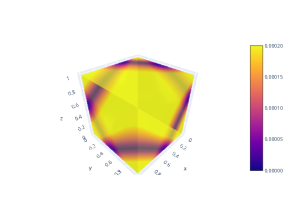
(f) Absolute error of SGL-3

(g) Predicted solution of TS-MGDL

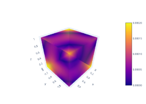
(h) Absolute error of TS-MGDL

Figure 12: Comparison between SGL methods and TS-MGDL method for the 3D Burgers equation at $t=1$.

In summary, the experimental results for the three examples presented above confirm that the proposed TS-MGDL method enables effective learning of solutions of the Burgers equations and outperforms existing single-grade deep learning methods in predictive accuracy and convergence. In particular, the predictive errors of the single-grade deep learning are larger than those of the multi-grade deep learning in 26-60, 4-31, and 3-12 times, for the 1D, 2D, and 3D equations, respectively. The numerical experiments show that the proposed TS-MGDL method is particularly suitable to solve nonlinear PDEs whose solutions may have singularities, since the method can effectively catch the intrinsic multiscale components of the solutions near the singularities.

6 Conclusion

A major shortcoming of traditional deep neural networks is that their prediction accuracy fails to decrease as the network goes deeper. To address this challenge, we propose a novel two-stage multi-grade deep learning method designed specifically for solving nonlinear PDEs. While traditional deep neural networks can be classified as single-grade learning, our multi-grade deep learning model is comprised of a superposition of neural networks arranged in a stair-like formation, with each level corresponding to a specific learning grade. We have showed that each grade/stage of the proposed TS-MGDL method can reduce the value of the loss function. This fact has been further validated by numerical experiments. Our experimental results demonstrate that the multi-grade method significantly outperforms the corresponding single-grade method in terms of higher prediction accuracy. Therefore, our proposed multi-grade learning approach provides an innovative solution to overcome the limitations of traditional single-grade models.

The numerical experiments confirm that the proposed TS-MGDL method is particularly suitable for solving nonlinear PDEs whose solutions have singularities. Moreover, the numerical study presented in this paper demonstrates that DNNs can overcome the curse of dimensionality when solving PDEs. Although we have only tested our proposed TS-MGDL method on the Burgers equation, it can be widely applied in solving other types of nonlinear PDEs. While this paper mainly focuses on developing the computational methodology and considering its numerical implementation, it motivates us to envision several crucial related theoretical issues to be studied in future projects.

References

- [1] I. Babuška, U. Banerjee, and J. E. Osborn, Survey of meshless and generalized finite element methods: A unified approach, Acta Numerica, 12 (2003), pp. 1–125.
- [2] G. Bao, X. Ye, Y. Zang, and H. Zhou, Numerical solution of inverse problems by weak adversarial networks, Inverse Problems, 36 (2020), 115003.
- [3] C. Basdevant, M. Deville, P. Haldenwang, J. Lacroix, J. Ouazzani, R. Peyret, P. Orlandi, and A. Patera, Spectral and finite difference solutions of the burgers equation, Computers Fluids, 14 (1986), pp. 23–41.
- [4] L. Bottou, Stochastic Gradient Descent Tricks, Neural Networks: Tricks of the Trade: Second Edition, Springer, Berlin, Heidelberg, 2012, pp. 421–436.
- [5] S. C. Brenner, The Mathematical Theory of Finite Element Methods, Springer, New York, 2008.
- [6] Z. Chen, J. Wu, and Y. Xu, Higher-order finite volume methods for elliptic boundary value problems, Advances in Computational Mathematics, 37 (2012), pp. 191–253.
- [7] Z. Chen, Y. Xu, and Y. Zhang, A construction of higher-order finite volume methods, Mathematics of Computation, 84 (2015), pp. 599–628.
- [8] D. Cheng, X. Tan, and T. Zeng, A dispersion minimizing finite difference scheme for the Helmholtz equation based on point-weighting, Computers & Mathematics with Applications, 73 (2017), pp. 2345–2359.
- [9] S. Cuomo, V. S. Di Cola, F. Giampaolo, G. Rozza, M. Raissi, and F. Piccialli, Scientific machine learning through physics–informed neural networks: where we are and what’s next, Journal of Scientific Computing, 92 (2022), 88.
- [10] I. Daubechies, R. DeVore, S. Foucart, B. Hanin, and G. Petrova, Nonlinear approximation and (deep) relu networks, Constructive Approximation, 55 (2022), pp. 127–172.
- [11] C. Deng, L. Ma, and T. Zeng, Crude oil price forecast based on deep transfer learning: Shanghai crude oil as an example, Sustainability, 13 (2021), 13770.
- [12] M. Diefenthaler, A. Farhat, A. Verbytskyi, and Y. Xu, Deeply learning deep inelastic scattering kinematics, The European Physical Journal C, 82 (2022), 1064.
- [13] W. E and B. Yu, The deep Ritz method: A deep learning-based numerical algorithm for solving variational problems, Communications in Mathematics and Statistics, 6 (2018), pp. 1–12.
- [14] H. Gao, L. Sun, and J. Wang, Phygeonet: Physics-informed geometry-adaptive convolutional neural networks for solving parameterized steady-state pdes on irregular domain, Journal of Computational Physics, 428 (2021), 110079.
- [15] I. Goodfellow, Y. Bengio, and A. Courville, Deep Learning, MIT Press, Cambridge, Massachusetts, 2017.
- [16] D. P. Kingma and J. Ba, Adam: A method for stochastic optimization, in 3rd International Conference on Learning Representations, ICLR 2015, San Diego, CA, USA, May 7-9, 2015, Conference Track Proceedings, Y. Bengio and Y. LeCun, eds., 2015.
- [17] R. Li, Z. Chen, and W. Wu, Generalized Difference Methods for Differential Equations: Numerical Analysis of Finite Volume Methods, vol. 226, CRC Press, New York, 2000.
- [18] D. C. Liu and J. Nocedal, On the limited memory BFGS method for large scale optimization, Mathematical Programming, 45 (1989), pp. 503–528.
- [19] J. Lu, Y. Liu, and C.-W. Shu, An oscillation-free discontinuous Galerkin method for scalar hyperbolic conservation laws, SIAM Journal on Numerical Analysis, 59 (2021), pp. 1299–1324.
- [20] L. Lu, X. Meng, Z. Mao, and G. E. Karniadakis, DeepXDE: A deep learning library for solving differential equations, SIAM Review, 63 (2021), pp. 208–228.
- [21] T. Poggio, H. Mhaskar, L. Rosasco, B. Miranda, and Q. Liao, Why and when can deep-but not shallow-networks avoid the curse of dimensionality: A review, International Journal of Automation and Computing, 14 (2017), pp. 503–519.
- [22] J. Qiu and C.-W. Shu, Finite difference WENO schemes with Lax–Wendroff-type time discretizations, SIAM Journal on Scientific Computing, 24 (2003), pp. 2185–2198.
- [23] M. Raissi, Deep hidden physics models: Deep learning of nonlinear partial differential equations, Journal of Machine Learning Research, 19 (2018), pp. 932–955.
- [24] M. Raissi, P. Perdikaris, and G. E. Karniadakis, Physics-informed neural networks: A deep learning framework for solving forward and inverse problems involving nonlinear partial differential equations, Journal of Computational Physics, 378 (2019), pp. 686–707.
- [25] J. Shen, T. Tang, and L. Wang, Spectral Methods: Algorithms, Analysis and Applications, vol. 41, Springer, Berlin, 2011.
- [26] Z. Shen, H. Yang, and S. Zhang, Deep network approximation characterized by number of neurons, Commun. Comput. Phys., 28 (2020), pp. 1768–1811.
- [27] J. Sirignano and K. Spiliopoulos, DGM: A deep learning algorithm for solving partial differential equations, Journal of Computational Physics, 375 (2018), pp. 1339–1364.
- [28] A. Vaswani, N. Shazeer, N. Parmar, J. Uszkoreit, L. Jones, A. N. Gomez, L. Kaiser, and I. Polosukhin, Attention is all you need, in Proceedings of the 31st International Conference on Neural Information Processing Systems, NIPS’17, Red Hook, NY, USA, 2017, Curran Associates Inc., pp. 6000–6010.
- [29] B. Wang, W. Zhang, and W. Cai, Multi-scale deep neural network (MscaleDNN) methods for oscillatory stokes flows in complex domains, Communications in Computational Physics, 28 (2020), pp. 2139–2157.
- [30] G. B. Whitham, Linear and Nonlinear Waves, John Wiley & Sons, New York, 2011.
- [31] T. T. Wong, W. S. Luk, and P. A. Heng, Sampling with Hammersley and Halton points, Journal of Graphics Tools, 2 (1997), pp. 9–24.
- [32] Y. Xu, Multi-grade deep learning, arXiv preprint arXiv:2302.00150, (2023).
- [33] Y. Xu, Successive affine learning for deep neural networks, arXiv preprint arXiv:2305.07996, (2023).
- [34] Y. Xu and T. Zeng, Sparse deep neural network for nonlinear partial differential equations, Numerical Mathematics: Theory, Methods and Applications, 16 (2023), pp. 58–78.
- [35] Y. Xu and H. Zhang, Convergence of deep convolutional neural networks, Neural Networks, 153 (2022), pp. 553–563.
- [36] D.-X. Zhou, Universality of deep convolutional neural networks, Applied and Computational Harmonic Analysis, 48 (2020), pp. 787–794.
- [37] D. Zou, R. Balan, and M. Singh, On lipschitz bounds of general convolutional neural networks, IEEE Transactions on Information Theory, 66 (2020), pp. 1738–1759.