Abstract

In cluster randomized experiments, units are often recruited after the random cluster assignment, and data are only available for the recruited sample. Post-randomization recruitment can lead to selection bias, inducing systematic differences between the overall and the recruited populations, and between the recruited intervention and control arms. In this setting, we define causal estimands for the overall and the recruited populations. We first show that if units select their cluster independently of the treatment assignment, cluster randomization implies individual randomization in the overall population. We then prove that under the assumption of ignorable recruitment, the average treatment effect on the recruited population can be consistently estimated from the recruited sample using inverse probability weighting. Generally we cannot identify the average treatment effect on the overall population. Nonetheless, we show, via a principal stratification formulation, that one can use weighting of the recruited sample to identify treatment effects on two meaningful subpopulations of the overall population: units who would be recruited into the study regardless of the assignment, and units who would be recruited in the study under treatment but not under control. We develop a corresponding estimation strategy and a sensitivity analysis method for checking the ignorable recruitment assumption.

keywords: causal inference, cluster randomized experiment, principal stratification, selection bias, weighting

1.   Introduction

Randomized experiments are the gold standard for evaluating the causal effect of treatments. Randomization guarantees that the treatment arms are comparable in both measured and unmeasured baseline covariates. However, when the inclusion of a unit, which we generically refer to as recruitment or enrollment herein, into a randomized experiment is determined after the treatment assignment, units can self-select whether to participate in the experiment, inducing post-randomization selection bias. This problem is prevalent in cluster randomized experiments, where all units in a cluster receive the same treatment. For example, health care studies often adopt the cluster randomization design, but the subjects are typically recruited after the clusters are randomized and they are not blinded to the assignment (Turner et al., 2017). Patients are often more willing to participate in a specific treatment arm, especially when that treatment has a perceived benefit. Consequently, the recruited treatment and control arms can be systematically different, breaking the initial randomization. This type of selection bias is also known as recruitment or identification bias in the clinical trials literature (Hahn et al., 2005).

Post-randomization selection bias has important implications in the design and analysis of cluster randomized experiments (Li et al., 2022a). First, the recruited sample is generally not a simple random sample of the overall population; therefore, it is important to differentiate between the causal estimands defined on the recruited population and the overall population. Second, in the presence of post-randomization selection bias, one cannot correctly estimate the causal effect on the recruited population without additional assumptions (Schochet et al., 2022; Su and Ding, 2021). Furthermore, current methodology suggests that it is necessary to obtain additional data on at least a portion of the non-recruited units to validly estimate causal effects on the overall population (Li et al., 2022b). However, such additional data are usually not directly available in a given experiment.

Post-randomization selection bias is a special case of the general setting of an intermediate variable lying temporally between an exposure and an outcome (Rosenbaum, 1984; Frangakis and Rubin, 2002). Other cases include noncompliance (Angrist et al., 1996; Frangakis et al., 2002) and truncation-by-death (Ding et al., 2011). The recruitment bias setting is unique in that data on the unrecruited units are entirely missing, whereas many other settings have at least partial data on all units regardless of the value of the intermediate outcome. A natural question is that whether one can estimate meaningful causal estimands on the overall population based on the recruited sample alone. A similar problem arises in the observational studies of discrimination, where the exposure is race, the outcome is a criminal justice or socio-economic measure, and data is only available on the units having a certain intermediate outcome that may be affected by the exposure, such as being arrested (Gaebler et al., 2022; Zhao et al., 2022).

This paper contributes new identification results and methods to address selection bias in cluster randomized experiments. We first define estimands on the recruited and overall population, and subpopulations of interest (Section 2). We specify a condition under which cluster-level randomization implies individual-level randomization (Section 3.1). We show that, under an ignorability and a monotonicity assumption on the recruitment mechanism, one can nonparametrically identify, using only the recruited sample, the average treatment effect on (i) the recruited population, and (ii) two interpretable subpopulations of the overall population. (Section 3.2). The central tool is through weighting based on the working propensity score, which is the conditional probability of being in the treatment arm among the recruited units. We develop an estimation strategy and show the estimators are consistent and asymptotically normal (Section 4). We then develop a new sensitivity analysis method to assess the ignorable recruitment assumption (Section 5). We report a simulation study (Section 6) and illustrate the proposed methods with a real application in cardiology (Section 7).

2.   Causal Estimands

Consider a cluster randomized experiment which consists of $J$ clusters drawn from a super-population of clusters, among which $m$ clusters are randomized to the intervention arm, denoted by $Z_{j}^{c}=1$, and the rest clusters to the control arm, denoted by $Z_{j}^{c}=0$. The superscript ‘$c$’ emphasizes that it is a cluster-level variable. There are two scenarios of the units composition of a cluster, differing in whether the treatment assignment affects the units’ cluster membership. In the first scenario, the treatment assignment affects a unit’s choice of cluster. For example, in health care of rare diseases, patients might choose a hospital that is specialized in treating their conditions or offers a new experimental treatment that is perceived as beneficial. We do not consider this scenario, some discussion of which is offered in Schochet (2022) and Schochet (2023). In the second scenario, which is the focus of this paper, units do not self-select into a cluster based on the study rollout or the treatment assignment. For example, units in a classroom or village are usually fixed at the time of randomization and would remain in that cluster throughout the study. Another example is health care of common diseases such as heart disease or diabetes; patients usually choose a hospital based on distance or insurance and would not change hospitals. This is the case in our application (Section 7). We formalize this scenario below.

Assumption 1.

Let $\mathcal{J},\mathcal{J^{\prime}}$ denote two sets of clusters that could comprise the cluster randomized experiment, and $\bm{z}\in\{0,1\}^{|\mathcal{J}|},\bm{z}^{\prime}\in\{0,1\}^{|\mathcal{J}^{\prime}|}$ two hypothetical cluster treatment assignments in each composition, respectively. Let $Q(\mathcal{J},\bm{z})$ denote the cluster that a randomly chosen unit would belong to under cluster composition $\mathcal{J}$ and treatment assignment $\bm{z}$. We assume that $Q(\mathcal{J},\bm{z})=Q(\mathcal{J}^{\prime},\bm{z}^{\prime})$.

Under 1, if we conceive that units form a super-population and they arrive at the super-population of clusters under some random process, then this process is constant with respect to the study, and the units in the cluster randomized experiment can be considered fixed. We refer to all the units, recruited or not, across the clusters in the experiment as the overall population. 1 also allows us to use a double-index to denote clustered data: unit ‘$ij$’ denotes unit $i$ in cluster $j$ with the total number of units $N_{j}$. Under cluster randomization, all units in the same cluster have the same treatment, and $Z_{ij}=Z^{c}_{j}$. We use $N=\sum_{j}N_{j}$ to denote the number of units from the overall population in the study.

Though all the units in the overall population are eligible to participate in the experiment, each unit can decide whether to enroll into the study (i.e. consent to join the experiment and provide data) after randomization: $R_{ij}=1$ means enrolling and $R_{ij}=0$ otherwise. The subpopulation recruited into the study, i.e. the units with $R_{ij}=1$, is referred to as the recruited population, which is different from the overall population as long as $R_{ij}=0$ for some units. We denote the number of recruited units in cluster $j$ by $n_{j}\leq N_{j}$, and the total number of recruited units in the study by $n=\sum_{j}n_{j}$. Also, let $V_{ij}$ denote the individual $i$’s covariates and $V^{c}_{j}$ cluster $j$’s covariates. Let $X_{ij}=(V_{ij},V^{c}_{j})$ be the collection of covariates for unit $i$. Assuming SUTVA, for each unit $i$, there are two potential outcomes $Y_{ij}(0)$ and $Y_{ij}(1)$ as well as two potential recruitment statuses, $R_{ij}(0)$ and $R_{ij}(1)$. We only observe the covariates and the potential outcomes corresponding to the observed assignment of the recruited units, denoted as $Y_{ij}=Y_{ij}(Z_{ij})$ for those with $R_{ij}=R_{ij}(Z_{ij})=1$. In what follows, we always use ‘$\sum_{ij}$’ to denote a sum over the recruited units of all clusters.

We define the average treatment effect on the overall population as

$$\tau^{O}=\mathrm{E}\{Y_{ij}(1)-Y_{ij}(0)\}.$$

We also define the average treatment effect on the recruited population and its counterpart specific to treatment status $z(=0,1)$ as

$$\tau^{R}=\mathrm{E}\{Y_{ij}(1)-Y_{ij}(0)\mid R_{ij}=1\};\quad\tau^{R}_{z}=\mathrm{E}\{Y_{ij}(1)-Y_{ij}(0)\mid Z_{ij}=z,R_{ij}=1\},$$

respectively. The expectation is over the cluster superpopulation, from which the cluster information $\{V_{j}^{c},N_{j},\{V_{ij},R_{ij}(z),Y_{ij}(z)\}_{i=1}^{N_{j}}\}$ are $J$ i.i.d. draws. The estimand on the overall population $\tau^{O}$ and its counterparts on certain subpopulations of the overall population are usually the intended target estimands. However, researchers often resort to estimate $\tau^{R}$ because usually only data on the recruited sample are available. When the recruited sample is a simple random sample of the overall population or the treatment effect is homogeneous across all units, $\tau^{O}$ is equal to $\tau^{R}$, but not so otherwise.

We now introduce causal estimands on meaningful subpopulations of the overall population via a principal stratification formulation (Frangakis and Rubin, 2002). We will show that they are identifiable based on the recruited sample alone. Specifically, we classify the units in the overall population by their joint potential recruitment statuses under both assignments: $S_{ij}=(R_{ij}(0),R_{ij}(1))$; $S_{ij}$ is called a principal stratum. Due to the fundamental problem of causal inference, the individual principal stratum membership is not observable. Borrowing the nomenclature in the noncompliance literature (Angrist et al., 1996), we name the four principal strata as: $S_{ij}=(1,1)\equiv a$, always-recruited, units who would be recruited regardless of the assignment; $S_{ij}=(0,0)\equiv n$, never-recruited, units who would not be recruited regardless of the assignment; $S_{ij}=(0,1)\equiv c$, compliers, units who would be recruited under intervention but not under control; and $S_{ij}=(1,0)\equiv d$, defiers, units who would be recruited under control but not under intervention. By construction, principal stratum membership does not change by treatment assignment; therefore, we can define causal effects within each principal stratum, for example

$$\tau^{O}_{s}=\mathrm{E}\{Y_{ij}(1)-Y_{ij}(0)\mid S_{ij}=s\},$$ (1)

for $s\in\{a,n,c,d\}$. Let $\pi_{s}$ represent the proportion of principal stratum $s$ in the overall population, then $\tau^{O}$ is the weighted average of the stratum-specific effects across the strata: $\tau^{O}=\sum_{s}\pi_{s}\tau^{O}_{s}$. Also, we can define causal effects on unions of principal strata, $\tau^{O}_{a,c}=\mathrm{E}[Y_{ij}(1)-Y_{ij}(0)\mid S_{ij}\in\{a,c\}]$, which is equal to a weighted average of $\tau^{O}_{a}$ and $\tau^{O}_{c}$.

3.   Nonparametric identification

3.1   Identification Assumptions

Li et al. (2022a) showed that a simple difference in means estimator using the recruited sample is generally biased for both $\tau^{O}$ and $\tau^{R}$. In this section, we show how to nonparametrically identify the above causal estimands based on the recruited sample alone. We first need to formalize the random assignment of the clusters.

Assumption 2.

(Randomization). Let $Z^{c}=(Z^{c}_{1},Z^{c}_{2},\dots,Z^{c}_{J})$ denote the assignment of the clusters. Then, $\Pr\big{(}Z^{c}_{j}\mid Y_{ij}(0),Y_{ij}(1),V_{ij},V^{c}_{j}\text{ for all }{i,j}\big{)}=\Pr(Z^{c}_{j}).$

Under Assumptions 1 and 2, we can prove that cluster randomization implies individual randomization, as stated in the next lemma (the proof is in Supplement B).

Lemma 1.

If Assumptions 1 and 2 hold, then the unit-level treatment assignment on the overall population is as-if randomized at the individual level, and the probability of treatment of an individual unit is the same as the probability of treatment of the clusters, i.e. $\Pr(Z_{ij}=1\mid Y_{ij}(0),Y_{ij}(1),V_{ij},V^{c}_{j}\text{ for all }{i,j}\big{)}=\Pr(Z_{ij}=1)=\Pr(Z^{c}_{j}=1)$.

Assumption 1 characterizes the composition of the overall population. We now specify two closely related assumptions on the recruitment process to characterize the composition of the recruited population.

Assumption 3.A.

(Non-differential recruitment) The recruitment process is non-differential with respect to potential outcomes given covariates, i.e., there exists a function $\delta(x)$ such that

$$\delta(x)=\frac{\Pr(R_{ij}=1\mid Y_{ij}(0)=y_{0},Y_{ij}(1)=y_{1},X_{ij}=x,Z_{ij}=1)}{\Pr(R_{ij}=1\mid Y_{ij}(0)=y_{0},Y_{ij}(1)=y_{1},X_{ij}=x,Z_{ij}=0)},$$ (2)

for all $x,y_{0}$, and $y_{1}$.

Assumption 3.B.

(Ignorable recruitment) Conditional on covariates and the treatment assignment, an individual’s recruitment status is independent of the potential outcomes: $\Pr(R_{ij}=1\mid Y_{ij}(0),Y_{ij}(1),Z_{ij},X_{ij})=\Pr(R_{ij}=1\mid Z_{ij},X_{ij})$.

Assumption 3.A states that all factors driving the recruitment differently between treated and control units are measured, whereas Assumption 3.B states that all factors driving the recruitment are measured, i.e. there is no unmeasured confounding with respect to the recruitment process. Assumption 3.B implies Assumption 3.A, but not vice versa. As will be explained later, the function $\delta(x)$ is closely related to the proportion of units that belong to the different principal strata. 3.A is equivalent to the subset ignorability assumption in Gaebler et al. (2022): $Z_{ij}\perp\!\!\!\perp\{Y_{ij}(0),Y_{ij}(1)\}\mid\{X_{ij},R_{ij}=1\}$ (the proof is given in Supplement B.2). However, because treatment assignment temporally precedes recruitment, it is arguably hard to conceive and justify subset ignorability in our setting because it imposes the independence of the treatment assignment conditional on the post-assignment recruitment status.

We maintain a standard positivity assumption that ensures that the recruitment of any unit in the overall population is bounded away from 0.

Assumption 4 (Recruitment positivity).

There exists $\delta>0$ such that $\Pr(R_{ij}=1\mid Z_{ij}=z,X_{ij}=x)>\delta$ for all $(z,x)$.

3.2   Nonparametric Identification of Recruited and Overall Estimands

We first introduce the working propensity score, defined as the probability of being in the treatment group among the recruited units: $e({x})=\Pr(Z_{ij}=1\mid X_{ij}=x,R_{ij}=1).$ The working propensity score does not reflect the true treatment assignment mechanism (Rosenbaum and Rubin, 1983), but is rather a one-dimensional summary of the covariates of the recruited units. Its true value depends on the conditional distribution of the recruitment process through

$$e({x})=\frac{\Pr(R_{ij}=1\mid Z_{ij}=1,X_{ij}=x)}{\Pr(R_{ij}=1\mid X_{ij}=x)}\Pr(Z_{ij}=1),$$

which is unknown and cannot be estimated if there is no data on the un-recruited units. We discuss how to estimate the working propensity score in Section 4. If Assumption 4 holds, then the working propensity score is bounded away from 0 and 1 (see Supplement B.3).

With the recruited sample, $\tau^{R}$ is identifiable via the inverse probability weighting strategy, as follows. 3.A suffices in place of the stronger 3.B.

$$\tau^{R} =\mathrm{E}\left[\frac{Z_{ij}Y_{ij}}{e(X_{ij})}-\frac{(1-Z_{ij})Y_{ij}}{1-e(X_{ij})}\ \bigg{|}\ R_{ij}=1\right].$$ (3)

The proof is in Supplement B.4. Note that $\tau^{R}$ is also identifiable using the standard outcome modelling strategy. The identification formula for $\tau^{R}_{z}$ is similar, with the contribution of each unit multiplied by $e(X_{ij})$ for $\tau^{R}_{1}$ and by $1-e(X_{ij})$ for $\tau^{R}_{0}$ (Li et al., 2018).

We now show how to identify causal effect on two meaningful subpopulations of the overall population from the recruited sample alone. Notice that the observed cells of $(R,Z)$ consists of mixtures of principal strata. Specifically, the recruited treatment units $(Z_{ij}=1,R_{ij}=1)$ consist of compliers and always-recruited, whereas the recruited control units $(Z_{ij}=0,R_{ij}=1)$ consist of always-recruited and defiers. This observation connects two specific estimands for the overall population to specific estimands for the recruited population, summarized as follows.

Theorem 1.

If Assumptions 1, 2 and 3.B hold, we have (a) $\tau^{O}_{a,d}=\tau^{R}_{0}$, and (b) $\tau^{O}_{a,c}=\tau^{R}_{1}.$ If 4 also holds, the average treatment effect on the always- and defier-recruited units in the overall population, $\tau^{O}_{a,d}$, is identifiable as

$$\tau^{O}_{a,d}\equiv\mathrm{E}[Y_{ij}(1)-Y_{ij}(0)\mid S_{ij}\in\{a,d\}]=\mathrm{E}\left[\frac{Z_{ij}Y_{ij}\{1-e(X_{ij})\}}{e(X_{ij})}-(1-Z_{ij})Y_{ij}\bigg{|}R_{ij}=1\right],$$ (4)

and the average treatment effect among the always- and complier-recruited units in the overall population, $\tau^{O}_{a,c}$, is identifiable as

$$\tau^{O}_{a,c}\equiv\mathrm{E}[Y_{ij}(1)-Y_{ij}(0)\mid S_{ij}\in\{a,c\}]=\mathrm{E}\left[Z_{ij}Y_{ij}-\frac{(1-Z_{ij})Y_{ij}e(X_{ij})}{1-e(X_{ij})}\bigg{|}R_{ij}=1\right].$$ (5)

Equation 5 states that the causal effect on the union of always-recruited and defiers in the overall population is equal to the causal effect on the recruited control arm, and that the effect on the union of always-recruited and compliers in the overall population is equal to the effect on the recruited treated arm. The two causal estimands on the recruited population are identifiable via a weighting scheme that was originally designed for identifying average treatment effect for the treated and the control units in standard causal literature, respectively (Li et al., 2018). Consequently, the corresponding overall population estimands are also identifiable.

Equation 5 becomes further interpretable under a monotonicity assumption on the enrollment status (Angrist et al., 1996).

Assumption 5.

(Monotonicity of recruitment) $R_{ij}(1)\geq R_{ij}(0)$ for all units.

Monotonicity rules out defiers, so that the recruited control arm consists only of always-recruited units, and $\tau^{O}_{a,d}\equiv\tau^{O}_{a}$. Equation 5 implies a weighting-based identification strategy for $\tau^{O}_{a}$: re-weight the recruited treatment units by $\{1-e(X_{ij})\}/e(X_{ij})$ and leave the recruited control units as is. A similar weighting strategy allows us to identify the causal effect on the union of always- and complier-recruited units of the overall population, $\tau^{O}_{a,c}$ based on the recruited sample alone. Furthermore, because $\tau^{O}_{a,c}=\nu\tau^{O}_{a}+(1-\nu)\tau^{O}_{c}$ with $\nu={\pi_{a}}/(\pi_{a}+\pi_{c})$, we can identify $\tau^{O}_{c}$ as long as we can identify the relative proportions of always-recruited and compliers. The next theorem shows how to identify $\nu$ and consequently $\tau^{O}_{c}$.

Theorem 2.

If Assumptions 1, 2 and 5 hold, the proportion of always-recruited units among the always- and complier-recruited units of the overall population is identifiable as

$$\nu\equiv\frac{\pi_{a}}{\pi_{a}+\pi_{c}}=\frac{\pi^{t}(1-p^{t})}{(1-\pi^{t})p^{t}},$$ (6)

where $\pi^{t}=\Pr(Z=1)$ and $p^{t}=\Pr(Z=1\mid R=1)$ is the probability of treatment in the overall and the recruited population, respectively. If Assumptions 3.B and 4 also hold, the causal effect among the compliers is identifiable as $\tau^{O}_{c}=(\tau^{O}_{a,c}-\nu\tau^{O}_{a})/(1-\nu)$, with $\tau^{O}_{a,c},\tau^{O}_{a}$ being identified from Theorem 5.

We note that from Lemma 1, the probability of treatment in the overall population $\pi^{t}$ is equal to the probability of treatment for a cluster $P(Z^{c}=1)$, and therefore all quantities in Theorem 2 are identifiable.

4.   Estimation

4.1   Causal effect estimators

Given the identification formulas Equation 3, Equation 4 and Equation 5, we propose the corresponding Hajék weighting estimators for $\tau^{R}$, $\tau^{O}_{a}$ and $\tau^{O}_{a,c}$ using only the sample of recruited individuals:

$$\widehat{\tau}=\frac{\sum_{ij}w_{1}(X_{ij})Z_{ij}Y_{ij}}{\sum_{ij}w_{1}(X_{ij})Z_{ij}}-\frac{\sum_{ij}w_{0}(X_{ij})(1-Z_{ij})Y_{ij}}{\sum_{ij}w_{0}(X_{ij})(1-Z_{ij})},$$ (7)

with the weights $\{w_{0}(x)=1/(1-e(x)),w_{1}(x)=1/e(x)\}$ for $\tau^{R}$, $\{w_{0}(x)=1,w_{1}(x)=(1-e(x))/e(x)\}$ for $\tau^{O}_{a}$, and $\{w_{0}(x)=e(x)/(1-e(x)),w_{1}(x)=1\}$ for $\tau^{O}_{a,c}$. We estimate $\nu$ in Equation 6 by substituting the probabilities of treatment in the overall and recruited population with the randomization probability at the cluster level $\Pr(Z^{c}=1)$, and the proportion of treated individuals in the recruited sample, respectively. Then, we estimate $\tau^{O}_{c}$ using the estimators $\widehat{\nu}$, $\widehat{\tau}^{O}_{a}$ and $\widehat{\tau}^{O}_{a,c}$ based on Theorem 2. We show that the resulting causal estimators are consistent and asymptotically normal using M-estimation (Van der Vaart, 2000). The proof is in Supplement B.6.

Theorem 3.

If Assumptions 1, 2, 3.B, 4 and 5 hold, and under mild additional regularity conditions, we have $\displaystyle\sqrt{J}\big{(}(\widehat{\tau}_{a}^{O},\widehat{\tau}_{c}^{O},\widehat{\tau}^{R})^{\top}-({\tau}_{a}^{O},\tau_{c}^{O},\tau^{R})^{\top}\big{)}\rightarrow N(0,\Sigma),$ as $J\rightarrow\infty$ where the form of $\Sigma$ is given in the supplement.

4.2   Estimation of the working propensity score

In practice, the working propensity score $e(x)$ is usually unknown and is replaced by its estimates $\widehat{e}(x)$. Notice that the ratio of recruitment probability $\delta(x)$ defined in Equation 2 is related to the working propensity score $e(x)$ as $e({x})={\delta(x)}/\{\delta(x)+r^{-1}\},$ where $r=\Pr(Z^{c}=1)/\Pr(Z^{c}=0)$. Under monotonicity (5), we can show that $\delta(x)$ is related to the probability of principal stratum membership as

$$\delta(x)=\Pr(S=a\mid S\in\{a,c\},X=x)^{-1}\geq 1.$$

Therefore, a parametric specification can be placed on $\Pr(S=a\mid S\in\{a,c\},X=x)$, $\delta(x)$, or $e({x})$, but it must satisfy that $\delta(x)\geq 1$. The traditional approach to propensity score estimation is to specify a logistic model on $e({x})$. However, this model is not compatible with data from experiments with recruitment bias because it does not satisfy that $\delta(x)\geq 1$.

For that reason, we choose to specify $\delta(x)$ instead of $e(x)$. Specifying $\delta(x)$ also reflects the correct temporal order of the variables since the treatment occurs temporally before recruitment. We adopt a specification on $\Pr(S=a\mid S\in\{a,c\},X=x)$ based on parameters ${\alpha}$, which leads to a parametric specification on $\delta(x)$ and $e(x)$. For example, if we specify a logistic model $\displaystyle\Pr(S=a\mid S\in\{a,c\},X=x)=\mathrm{expit}\{x^{T}{\alpha}\}$, it implies that $\delta(x;{\alpha})=1+\exp\{-x^{T}{\alpha}\}$ and $\mathrm{logit}\ e({x};{\alpha})=\log\{r\delta(x;{\alpha})\}.$

Estimating the parameters of a working propensity score model, ${\alpha}$, in a cluster randomized experiment is complicated because all units within a cluster have the same treatment. We suggest to estimate ${\alpha}$ by maximizing the pseudo-likelihood for the treatment assignment among the recruited units: $\text{pseudo-}L(\alpha)=\prod_{ij}e(X_{ij};{\alpha})^{Z_{ij}}[1-e(X_{ij};{\alpha})]^{1-Z_{ij}},$ which under the specification above becomes: $\text{pseudo-}L(\alpha)=\prod_{ij}\log\{r\delta(X_{ij};{\alpha})\}^{Z_{ij}}[1-\log\{r\delta(x;{\alpha})\}]^{1-Z_{ij}}.$ A standard optimizer can be used to find the maximizer of the pseudo-likelihood $\widehat{\alpha}$. We use the function optim in R. We have found in simulations that this approach leads to consistent estimators for the working propensity score parameters, and consequent weighting estimators for the causal effects (Section 6). Extending the asymptotic distributions for the causal estimators in Theorem 3 to the case with the estimated propensity scores can be readily achieved by modifying the estimating function to include the pseudo-likelihood contribution for each cluster. From simulations in Section 6, we found that a bootstrap procedure that resamples clusters performs well for inference based on the true and estimated working propensity scores.

Alternative specifications of $\delta(x)$ can be considered, as long as they impose that $\delta(x)\geq 1$.

5.   Sensitivity analysis

The ignorable recruitment (Assumption 3.B) is central to identifying causal effects for the overall population. We develop a sensitivity analysis to assess this assumption within the Rosenbaum’s bounds framework (Rosenbaum, 2002). Specifically, assume there exists an unmeasured covariate $U$ that is necessary for Assumption 3.B to hold, that is, $R\perp\!\!\!\perp\{Y(0),Y(1)\}\mid\{U,X,Z\}$, but $R\not\!\perp\!\!\!\perp\{Y(0),Y(1)\}\mid\{X,Z\}$. Then, consistent estimation of the causal effects requires that we use

$$\delta^{*}(x,u)=\frac{\Pr(R=1\mid U=u,X=x,Z=1)}{\Pr(R=1\mid U=u,X=x,Z=0)},$$

and the corresponding working propensity score $e^{*}(x,u)$, instead of $\delta(x)$ and $e({x})$. We consider violations to the ignorable recruitment assumption with respect to $U$ up to a factor $\Gamma$ (the sensitivity parameter) as

$$\Gamma^{-1}\leq\rho(x,u)={\delta(x)}\ /\ {\delta^{*}(x,u)}\leq\Gamma.$$ (8)

A larger value of $\Gamma$ allows a greater degree of violation. To conduct a sensitivity analysis, we need to bound the chosen estimator for each fixed value of $\Gamma$. We focus on the Hajék estimator Equation 7, which is more efficient than the Horvitz-Thompson estimator, but is technically more challenging for sensitivity analysis (Aronow and Lee, 2013; Papadogeorgou et al., 2022).

For the causal effect on the always-recruited, $\tau^{O}_{a}$, the weights of the control units are equal to 1. Therefore it suffices to focus on the part of the estimator corresponding to the treated units. Denote the weights for the treated units in the estimator in Equation 7 for $\tau^{O}_{a}$ as $w_{1ij}^{*}=w_{1}^{*}(X_{ij},U_{ij})=\{1-e^{*}(X_{ij},U_{ij})\}/e^{*}(X_{ij},U_{ij})$. The following proposition provides an algorithm to acquire the bounds of the estimator for violations of the ignorable recruitment assumption up to $\Gamma$.

Proposition 1.

Maximizing (minimizing) $\tau^{*}_{1}=\frac{\sum_{ij}w_{1ij}^{*}Z_{ij}Y_{ij}}{\sum_{ij}w_{1ij}^{*}Z_{ij}}$ under the $\Gamma-$violation in Equation 8 is equivalent to solving the linear program that maximizes (minimizing) $\sum_{ij}\lambda_{ij}{w}_{1ij}Z_{ij}Y_{ij}$ with respect to $\lambda_{ij}$ subject to three constraints: (a) ${\kappa}{\Gamma^{-1}}\leq\lambda_{ij}\leq\kappa\Gamma$ (b) $\sum_{ij}\lambda_{ij}{w}_{1ij}Z_{ij}=1,$and (c) $\kappa\geq 0,$ where ${w}_{1ij}=w_{1}(X_{ij})$ is the weight of unit $i$ under treatment and working propensity score $e(x)$, and $\kappa$ is a parameter of the linear program.

Bounding the causal effect on the compliers is more complicated because it involves a non-linear optimization problem. Instead, we acquire bounds for the causal effect estimator of the union of the always- and complier-recruited units, $\widehat{\tau}^{O}_{a,c}$, using a procedure similar to the one in Proposition 1. Then, the bounds for the two estimators are combined according to the formula in Theorem 2 to form bounds for the causal estimator for the complier effect. This procedure is computationally fast because it only requires solving two relatively simple linear programs. It leads to conservative bounds under the $\Gamma$-violation of the ignorability assumption in the sense that the resulting bounds are no narrower than the sharp bounds that would be obtained via directly optimizing the causal effects of the compliers. More details are given in the Supplement B.7.

6.   Simulations

We performed simulations to study the differences between the causal estimands in the overall and recruited populations and evaluate the properties of the estimators proposed in Section 4.

Table 1: Specifications of the data generative models for the 36 simulation scenarios. Each scenario corresponds to a different combination of principal strata prevalences, covariate differences in always and complier-recruited, treatment proportion, and number of clusters.

Principal strata prevalences	Scenario A	20% Always, 20% Complier, 60% Never
	Scenario B	25% Always, 25% Complier, 50% Never
	Scenario C	15% Always, 25% Complier, 60% Never
Covariate separation of always-	Case 1	Strong
and complier-recruited	Case 2	Moderate
Treatment proportion	Balanced	Probability of cluster begin treated is 50%
	Imbalanced	Probability of cluster begin treated is 25%
Number of clusters $J$	200, 500, or 800

We considered 36 simulation scenarios, described in Table 1. In each scenario, we generated $J$ clusters of size 100 in their overall population. The cluster-level treatment was assigned with probability 0.5 or 0.25, representing balanced and imbalanced study designs, respectively. The proportion of recruited units depended on the specific generative model and varied from 21% to 38% with the proportion of the subgroup of treated units varying from 40% to 73%. Data under Scenario B and C had the highest and lowest proportion of recruitment, respectively, and data under Scenarios A and B had the same prevalence of treatment within the recruited population. We considered three unit-level and two cluster-level covariates. We generated outcomes with treatment effect heterogeneity and moderate intraclass correlation equal to 0.1. The true overall average treatment effect was 3, the average treatment effect among the recruited units varied from 2.71 to 2.81, among the always-recruited units from 2.64 to 2.68, and among the compliers from 2.88 to 3.07 across the 36 scenarios. This illustrates that the causal effects differ among the different populations of interest. The average effect among the recruited varied with the treatment probability since the corresponding population changes, even though the average effect on the overall or the always-recruited populations are constant. This illustrates that estimates on the recruited population are less interpretable, since their interpretation is driven by the experimental design. The specific data generative model for all scenarios is given in Supplement C.1.

We evaluated the estimators in terms of bias, variance and coverage of 95% confidence intervals. We considered interval estimators based on the asymptotic theory in Theorem 3 for the known propensity score, and based on a nonparametric bootstrap procedure that resamples clusters for the estimated propensity score. We discuss all the results here, though some figures are included in Supplement C.2 due to space constraints.

The naïve estimator which is defined as the difference of mean outcomes among the treated recruited and the control recruited individuals was biased for all estimands and across all configurations (Figure S.1). The proportion of always-recruited among the always- and complier-recruited in Equation 6 is well-estimated across data sets (Figure S.3), and the pseudo-likelihood estimators for the working propensity score parameters are unbiased with increasing precision under a larger number of clusters (Figure S.6). Figure 1 shows the difference between the estimated and the true causal effect when using the proposed estimators based on the estimated working propensity score model across 500 simulated data sets and the various simulation configurations under a balanced design. We see that the causal estimators for the effect on the recruited, the always-recruited, and the complier-recruited units are unbiased throughout, and they are more precise when the number of clusters increases. This illustrates that our approach accurately estimates the causal effect for the recruited population, and two meaningful subsets of the overall population. The causal estimators based on the true propensity score, or in imbalanced designs are also essentially unbiased, shown in the supplement.

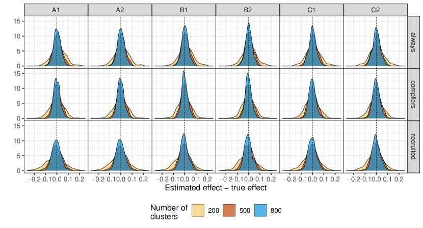
Figure 1: True minus estimated causal effect among the always-recruited, the complier-recruited, and the recruited populations, across 500 data sets and under the 6 scenario-case configurations, and 3 choices for the number of clusters, when the probability of cluster treatment is 0.5.

The coverage of the asymptotic 95% intervals for the estimator that uses the known propensity score varied from 90 to 97% across all scenarios and estimands. For the bootstrap procedure, we re-sampled clusters while holding the proportion of treated clusters fixed to maintain the overall prevalence of treatment, and created confidence intervals using the standard deviation of the bootstrap estimates. The coverage of the normality-based 95% intervals varied from 92.7 to 98.6% for the estimands on the recruited, and the always-recruited populations. Coverage of 95% intervals based on the bootstrap was lower but still reasonable for the average causal effect on the compliers, ranging from 85 to 93%. A figure for the coverage across simulation configurations is shown in the supplement.

7.   Application

We apply the proposed methods to evaluate the ARTEMIS (The Affordability and Real-World Antiplatelet Treatment Effectiveness AfterMyocardial Infarction Study) randomized clinical trial (Wang et al., 2019). The ARTEMIS trial aims to evaluate whether removing co-payment barriers increases the persistence of P2Y₁₂ inhibitor, which is a common drug for patients who had experienced myocardial infarction, and lowers risk of major adverse cardiovascular events. The intervention is randomized at the hospital level, where the intervention hospitals offered vouchers for patients to reimburse their co-payment of P2Y₁₂, whereas the control hospitals offered nothing. Because the intervention is an obvious incentive to the patients, this causes enrolling patients in the control hospitals much more challenging than the intervention hospitals, and renders the monotonicity assumption plausible.

Among the original 10,976 patients, we excluded hospitals whose sample size is less than 15, resulting in a final sample size of 10,400 from 203 hospitals with 108 intervention hospitals with 6,254 patients in total and 95 control hospitals with 4,146 patients in total. We compared the covariate distribution for hospital- and patient-level covariates among recruited patients, and found that a number of important covariates, e.g. race, education and prior P2Y₁₂ use, were imbalanced between the intervention and control groups. Details are given in Supplement D. This observation implies potential differential recruitment.

We focused on the outcome of medication persistence. An outcome equal to 1 means that the patient continued on the medication. The difference of the mean outcome among the recruited treated and control patients is $2.75\%$ with 95% confidence interval $(0.59,5.05)\%$. We estimated the working propensity score model based on the pseudo-likelihood technique detailed in Section 4.2 and using all the available covariates listed in Table S.3 of the Supplement. Using the proposed method, we estimated the proportion (and 95% confidence interval) of always-recruited among the always- and complier-recruited individuals to be $\widehat{\nu}=0.754$ (95% CI: $0.56$ to $1$), and the causal effect on the always-recruited to be $2.83\%$ (95% CI: $0.87$ to $4.75\%$), on the complier-recruited to be $2.63\%$ (95% CI: $-3.55$ to $4.41\%$), and on the recruited population to be $2.80\%$ (95% CI: $0.6$ to $4.44\%$). The results imply heterogeneous treatment effects: the voucher increases P2Y₁₂ medication persistence among the always-recruited patients, but does not have an effect among the compliers. Therefore, the effect in the recruited population is largely driven by the always-recruited subpopulation. This suggests that, to achieve better medication persistence, resources should be allocated to the always-recruited patients, who are arguably more motivated to take the medication. However, we found that these results are potentially sensitive to the violations of the ignorable recruitment assumption, with minimum $\Gamma$ value for which the bounds include zero equal to 1.13 for the always-recruited, and only 1.02 for the complier-recruited.

8.   Discussion

Due to the logistics and practical constraints, cluster randomized experiments are prone to post-randomization selection bias. In this paper, we established the conditions under which cluster randomization implies individual randomization. We clarified the different target populations and corresponding estimands, and provided weighting-based nonparametric identification formulas for these estimands based solely on the recruited sample and associated estimation strategies. Our identification critically relies on the ignorable recruitment assignment, which assumes away unmeasured confounding in the recruitment process. This assumption is intrinsically connected to, but different from, the principal ignorability assumption (Jo and Stuart, 2009; Ding and Lu, 2017; Jiang et al., 2022) in principal stratification. We also devised an interpretable sensitivity analysis method to assess the impact of the ignorable recruitment assumption.

We have focused on addressing the identification challenges due to non-random recruitment, but assumed away other potential complications that might arise in cluster randomized experiments. First, we have operated under the assumption of constant cluster membership such that the treatment assignment does not affect individual’s choice of clusters. This assumption effectively reduces the number of possible principal strata and is plausible in scenarios where the sampling frame for each cluster is determined before the start of the study and thus the cluster membership is a pre-treatment characteristic. Schochet (2022, 2023) discussed scenarios where the treatment assignment affects cluster membership, in which case the causal estimands would need to be redefined and stronger identification assumptions are invoked for point identification. It would be desirable to expand our work to address treatment-dependent cluster membership and sensitivity methods for potentially stronger assumptions. Second, we operate under the assumption of non-informative cluster size, such that the expectation of individual-level potential outcomes contrast is well-defined. Under informative cluster sizes, there can be different definitions of a treatment effect estimand, depending on whether each individual or each cluster is given an equal weight (Papadogeorgou et al., 2019; Kahan et al., 2023; Wang et al., 2022). In future work, we plan to pursue identification results for our estimands when the cluster sizes are informative.

Supplementary materials for
“Addressing selection bias in cluster randomized experiments via weighting”
by
Georgia Papadogeorgou, Bo Liu, Fan Li, Fan Li

Appendix A Notation

To facilitate clear presentation, we first list in LABEL:supp_tab:notation the notation that is used throughout the manuscript and supplement.

Table S.1: Glossary of notation.

$J$	Total number of clusters
$Z^{c}_{j},V^{c}_{j}$	Cluster level treatment and covariates
$N_{j},N$	Number of units in the overall population for cluster $j$ and in all the clusters
$n_{j},n$	Number of recruited units cluster $j$ and in all the clusters
$Z_{ij},V_{ij},X_{ij}$	Unit-level treatment, covariates, and the vector of both unit and cluster-level covariates
$R_{ij}(0),R_{ij}(1),R_{ij}$	Potential and observed values of the unit-level recruitment
$Y_{ij}(0),Y_{ij}(1),Y_{ij}$	Potential and observed values of the outcome
$\tau^{O},\tau^{R}$	Average effects on the overall and recruited populations
$\tau^{R}_{z}$	Average effect on the recruited populations with treatment level $z$
$\tau^{O}_{s}$	Average effects for units in the overall population with recruitment principal stratum $S=s$
$\sum_{ij}$	Represents a sum over the recruited units, for example $\sum_{ij}Y_{ij}=\sum_{j=1}^{J}\sum_{i=1}^{n_{j}}R_{ij}Y_{ij}$

We use $i\in j$ to denote the units within cluster $j$ (recruited or not), and $i\in j^{*}$ to denote the recruited subjects in cluster $i$. Then, summations of the form $\sum_{i=1}^{N}$ can be re-written as $\sum_{j=1}^{J}\sum_{i\in j}$, and the summations of the form $\sum_{i=1}^{n}$ can be re-written as $\sum_{j=1}^{J}\sum_{i\in j^{*}}$.

Appendix B Proofs

B.1   Randomized treatment on the overall population

Proof of Lemma 1.

Here, it is more convenient to use the single index notation. Specifically, let $i=1,2,\dots,N$ denote a randomly chosen unit in the overall population of the $J$ clusters, and let $Q_{i}=j$ denote that unit $i$ belongs to cluster $j$. First, we start by showing that the cluster-level randomization of treatment, also implies that the cluster-level treatment is independent of cluster memberships (based on 1), formalized as:

$$\Pr(Z^{c}_{j}=1\mid\{V^{c}_{j}\}_{j=1}^{J},\{V_{i},Y_{i}(0),Y_{i}(1)\}_{i=1}^{N},Q_{i})=\Pr(Z^{c}_{j}=1).$$ (S.1)

In other words, knowing which cluster subject $i$ belongs to does not provide any information on the cluster treatment level. Note that 1 implies that, among the overall population,

$$\Pr(Q_{i}=j\mid\{Z_{j}^{c},V^{c}_{j}\}_{j=1}^{J},\{V_{i},Y_{i}(0),Y_{i}(1)\}_{i=1}^{N})=\Pr(Q_{i}=j\mid\{V^{c}_{j}\}_{j=1}^{J},\{V_{i},Y_{i}(0),Y_{i}(1)\}_{i=1}^{N}).$$

Then

$$\Pr(Z^{c}_{j}=1 \mid\{V^{c}_{j}\}_{j=1}^{J},\{V_{i},Y_{i}(0),Y_{i}(1)\}_{i=1}^{N},Q_{i})$$

$$=\frac{\Pr(Q_{i}\mid Z^{c}_{j}=1,\{V^{c}_{j}\}_{j=1}^{J},\{V_{i},Y_{i}(0),Y_{i}(1)\}_{i=1}^{N})}{\Pr(\{V^{c}_{j}\}_{j=1}^{J},\{V_{i},Y_{i}(0),Y_{i}(1)\}_{i=1}^{N},Q_{i})}\times$$

$$\hskip 30.0pt\times\Pr(Z^{c}_{j}=1\mid\{V^{c}_{j}\}_{j=1}^{J},\{V_{i},Y_{i}(0),Y_{i}(1)\}_{i=1}^{N})\ \Pr(\{V^{c}_{j}\}_{j=1}^{J},\{V_{i},Y_{i}(0),Y_{i}(1)\}_{i=1}^{N})$$

$$=\frac{\Pr(Q_{i}\mid\{V^{c}_{j}\}_{j=1}^{J},\{V_{i},Y_{i}(0),Y_{i}(1)\}_{i=1}^{N})}{\Pr(\{V^{c}_{j}\}_{j=1}^{J},\{V_{i},Y_{i}(0),Y_{i}(1)\}_{i=1}^{N},Q_{i})}\times$$ (From 1)

$$\hskip 30.0pt\times\Pr(Z^{c}_{j}=1\mid\{V^{c}_{j}\}_{j=1}^{J},\{V_{i},Y_{i}(0),Y_{i}(1)\}_{i=1}^{N})\ \Pr(\{V^{c}_{j}\}_{j=1}^{J},\{V_{i},Y_{i}(0),Y_{i}(1)\}_{i=1}^{N})$$

$$=\Pr(Z^{c}_{j}=1)$$ (From 2)

We have:

$$\Pr(Z_{i}=1\mid\{V^{c}_{j}\}_{j=1}^{J},\{V_{i},Y_{i}(0),Y_{i}(1)\}_{i=1}^{N})=$$

$$=\sum_{j=1}^{J}\Pr(Z_{i}=1\mid\{V^{c}_{j}\}_{j=1}^{J},\{V_{i},Y_{i}(0),Y_{i}(1)\}_{i=1}^{N},Q_{i}=j)\Pr(Q_{i}=j\mid\{V^{c}_{j}\}_{j=1}^{J},\{V_{i},Y_{i}(0),Y_{i}(1)\}_{i=1}^{N})$$

$$=\sum_{j=1}^{J}\Pr(Z^{c}_{j}=1\mid\{V^{c}_{j}\}_{j=1}^{J},\{V_{i},Y_{i}(0),Y_{i}(1)\}_{i=1}^{N},Q_{i}=j)\Pr(Q_{i}=j\mid\{V^{c}_{j}\}_{j=1}^{J},\{V_{i},Y_{i}(0),Y_{i}(1)\}_{i=1}^{N})$$

$$=\Pr(Z^{c}_{j}=1)\sum_{j=1}^{J}P(Q_{i}=j\mid\{V^{c}_{j}\}_{j=1}^{J},\{V_{i},Y_{i}(0),Y_{i}(1)\}_{i=1}^{N})$$ (From Equation S.1)

$$=\Pr(Z^{c}_{j}=1)$$

Further, Equation S.1 implies that $\Pr(Z^{c}_{j}=1\mid Q_{i})=\Pr(Z^{c}_{j}=1)$ and in turn

$$\Pr(Z_{i}=1) =\sum_{j=1}^{J}P(Z_{i}=1\mid Q_{i}=j)\Pr(Q_{i}=j)$$

$$=\sum_{j=1}^{J}P(Z^{c}_{j}=1\mid Q_{i}=j)\Pr(Q_{i}=j)$$

$$=\Pr(Z^{c}_{j}=1)\sum_{j=1}^{J}\Pr(Q_{i}=j)$$ (From Equation S.1)

$$=\Pr(Z^{c}_{j}=1).$$

Putting these together: $\Pr(Z_{i}=1\mid\{V^{c}_{j}\}_{j=1}^{J},\{V_{i},Y_{i}(0),Y_{i}(1)\}_{i=1}^{N})=P(Z_{i}=1)=P(Z^{c}_{j}=1)$.

∎

B.2    Relationships among assumptions for post-treatment recruitment

Proposition S.1.

3.A is equivalent to subset ignorability, $Z\perp\!\!\!\perp Y(0),Y(1)\mid X,R=1$. When 3.B holds, 3.A also holds, though the reverse is not true.

Proof.

First we show that 3.A $\implies$ $Z\perp\!\!\!\perp Y(0),Y(1)\mid X,R=1$. We denote $f_{\mathbf{Y}(\cdot)}$ as the distribution of $\mathbf{Y}(\cdot)=(Y(0),Y(1))$ and $\mathbf{y}(\cdot)$ as one realization.

$$f_{\mathbf{Y}(\cdot)} (\mathbf{y}(\cdot)\mid R=1,Z=z,X={x})$$

$$=\frac{P(R=1\mid Z=z,X={x},\mathbf{Y}(\cdot)=\mathbf{y}(\cdot))P(Z=z\mid X={x},\mathbf{Y}(\cdot)=\mathbf{y}(\cdot))f_{\mathbf{Y}(\cdot)}(\mathbf{y}(\cdot)\mid X={x})}{P(R=1\mid Z=z,X={x})P(Z=z\mid X={x})}$$

$$=\frac{P(R=1\mid Z=z,X={x},\mathbf{Y}(\cdot)=\mathbf{y}(\cdot))}{P(R=1\mid Z=z,X={x})}f_{\mathbf{Y}(\cdot)}(\mathbf{y}(\cdot)\mid X={x}),$$ (Randomized treatment in the overall population – See Lemma 1)

From 3.A,

$$P(R=1 \mid Z=1,X={x})=$$

$$=\int P(R=1\mid Z=1,X={x},\mathbf{Y}(\cdot)=\mathbf{y}(\cdot))f_{\mathbf{Y}(\cdot)}(\mathbf{y}(\cdot)\mid Z=1,X={x})\mathrm{d}\mathbf{y}(\cdot)$$

$$=\delta({x})\int P(R=1\mid Z=0,X={x},\mathbf{Y}(\cdot)=\mathbf{y}(\cdot))f_{\mathbf{Y}(\cdot)}(\mathbf{y}(\cdot)\mid Z=0,X={x})\mathrm{d}\mathbf{y}(\cdot)$$ (Randomized treatment)

$$=\delta({x})P(R=1\mid Z=0,X={x})$$

Therefore,

$$f_{\mathbf{Y}(\cdot)} (\mathbf{y}(\cdot)\mid R=1,Z=1,X={x})=$$

$$=\frac{\delta({x})P(R=1\mid Z=0,X={x},\mathbf{Y}(\cdot)=\mathbf{y}(\cdot))}{\delta({x})P(R=1\mid Z=0,X={x})}f_{\mathbf{Y}(\cdot)}(\mathbf{y}(\cdot)\mid X={x})$$

$$=f_{\mathbf{Y}(\cdot)}(\mathbf{y}(\cdot)\mid R=1,Z=0,X={x}),$$

which gives us that $Z\perp\!\!\!\perp Y(0),Y(1)\mid X,R=1$.
Next we show that $Z\perp\!\!\!\perp Y(0),Y(1)\mid X,R=1$ $\implies$ 3.A. Consider

$$\frac{P(R=1\mid X,Y(0),Y(1),Z=1)}{P(R=1\mid X,Y(0),Y(1),Z=0)}=$$

$$=\frac{P(Z=1\mid X,Y(0),Y(1),R=1)P(R=1\mid X,Y(0),Y(1))\ \big{/}\ P(Z=1\mid X,Y(0),Y(1))}{P(Z=0\mid X,Y(0),Y(1),R=1)P(R=1\mid X,Y(0),Y(1))\ \big{/}\ P(Z=0\mid X,Y(0),Y(1))}$$

$$=\frac{P(Z=1\mid X,Y(0),Y(1),R=1)}{P(Z=0\mid X,Y(0),Y(1),R=1)}\frac{P(Z=0\mid X,Y(0),Y(1))}{P(Z=1\mid X,Y(0),Y(1))}$$

$$=\frac{P(Z=1\mid X,R=1)}{P(Z=0\mid X,R=1)}\frac{P(Z=0)}{P(Z=1)},$$

where the last equation holds from subset ignorability for the first ratio, and from Lemma 1 for the second ratio. Therefore, the ratio of enrollment probabilities is only a function of the covariates and 3.A is satisfied.
Next we show that 3.B implies 3.A. From 3.B we have that

$$\frac{P(R=1\mid X,Y(0),Y(1),Z=1)}{P(R=1\mid X,Y(0),Y(1),Z=0)}=\frac{P(R=1\mid X,Z=1)}{P(R=1\mid X,Z=0)}$$

is only a function of covariates and 3.A is satisfied.
The reverse is not true, and 3.A does not imply 3.B. The following example is a situation where 3.A holds, and 3.B does not. For a binary outcome, assume that

$$P(R=1\mid X,Y(0),Y(1),Z)=\begin{cases}0.5&\text{if }Y(0)=0\text{ and }Z=1,\\ 0.2&\text{if }Y(0)=0\text{ and }Z=0,\\ 0.75&\text{if }Y(0)=1\text{ and }Z=1,\\ 0.3&\text{if }Y(0)=1\text{ and }Z=1.\end{cases}$$

∎

B.3   The working propensity score

We show that enrollment positivity leads to working propensity score positivity.

Proposition S.2 (Working propensity score positivity).

If 4 holds, then there exists $\delta^{\prime}>0$ such that $\delta^{\prime}<e({x})<1-\delta^{\prime}$ for all ${x}$.

Proof.

Remember that

$$e({x}) =\frac{P(R=1\mid Z=1,X={x})}{\mathrm{P}(R=1\mid X={x})}\mathrm{P}(Z=1).$$

From 4 we have that $P(R=1\mid Z=z,X={x})>\delta$, which gives us that $\displaystyle e({x})>\delta P(Z=1).$ It also implies that $P(R=1\mid X={x})>\delta$, which in turn gives us that $\displaystyle e({x})<P(Z=1)/\delta.$ By setting $\delta^{\prime}=\min\{\delta P(Z=1),1-P(Z=1)/\delta\}$, we have the result. ∎

B.4   Identifiability of average causal effects for the recruited population

Here, we use the equivalence between weighting and conditioning estimands for our proof. The weighted average causal effect among a subpopulation of the recruited population with covariate distribution $g^{R}(x)$ is defined as

$$\tau^{R}_{g}=\mathrm{E}[h^{R}(X)[Y(1)-Y(0)]\mid R=1],$$

where $h^{R}(x)=g^{R}(x)/f^{R}(x)$, and $f^{R}(x)$ is the covariate distribution among the recruited units. For $g^{R}(x)=f^{R}(x)$, we have that $\tau_{g}^{R}=\tau^{R}$. Also, for $g^{R}(x)=f(x\mid Z=1,R=1)$ or $g^{R}(x)=f(x\mid Z=0,R=1)$, the estimand $\tau_{g}^{R}$ reverts to the average causal effect among the treated recruited units $\tau^{R}_{1}$ or the control recruited units $\tau^{R}_{0}$, respectively.

Proposition S.3.

If Assumptions 1, 2, 3.A, and 4 hold, then

$$\tau^{R}_{g} =\mathrm{E}\left[h^{R}(X)\left\{\frac{ZY}{e(X)}-\frac{(1-Z)Y}{1-e(X)}\right\}\bigg{|}R=1\right],$$

for any subpopulation of the recruited population with covariate distribution $g^{R}(x)$ and corresponding tilting function $h^{R}(x)$.

Proof.

We have

$$\mathrm{E}\left\{h^{R}(X)\frac{ZY}{e(X)}\mid R=1\right\} =\mathrm{E}\left\{\mathrm{E}\left[h^{R}(X)\frac{ZY(1)}{e(X)}\mid X,Y(1),Y(0),R=1\right]\mid R=1\right\}$$

$$=\mathrm{E}\left\{\frac{h^{R}(X)}{e(X)}Y(1)\ \mathrm{E}\left[Z\mid X,Y(1),Y(0),R=1\right]\mid R=1\right\}$$

$$=\mathrm{E}\left\{\frac{h^{R}(X)}{e(X)}Y(1)\ P(Z=1\mid X,Y(1),Y(0),R=1)\mid R=1\right\}$$

$$=\mathrm{E}\left\{\frac{h^{R}(X)}{e(X)}Y(1)\ P(Z=1\mid X,R=1)\mid R=1\right\}$$ (From Proposition S.1 & using 3.A)

$$=\mathrm{E}\left\{h^{R}(X)\ Y(1)\mid R=1\right\}$$

and similarly we can get that

$$\mathrm{E}\left\{h^{R}(X)\frac{(1-Z)Y}{1-e(X)}\mid R=1\right\}=\mathrm{E}\left\{h^{R}(X)\ Y(0)\mid R=1\right\},$$

which verifies the weighting-based identification formula.

∎

B.5   Identifiability of average causal effects for the overall population

We similarly use weighting definitions of estimands for the overall population for our proofs. The weighted average causal effect among a subpopulation of the overall population with covariate distribution $g^{O}(x)$ is defined as $\tau^{O}_{g}=\mathrm{E}\left[h^{O}(X)[Y(1)-Y(0)]\right],$ where $h^{O}(x)=g^{O}(x)/f_{X}(x)$, and $f_{X}(x)$ is the covariate distribution in the overall population. For $g^{O}(x)=f_{X}(x)$, we have that $\tau_{g}^{O}=\tau^{O}$. Also, for $g^{O}(x)=f(x\mid S\in\{a,d\})$, the estimand $\tau_{g}^{O}$ reverts to the average causal effect among the always- and defier-recruited units $\tau^{O}_{a,d}$, and similarly for the other principal strata.

Proof of Equation 5.

First, we establish how probabilistic statements about the recruitment indicator $R$ given treatment can be linked to probabilistic statements about the potential recruitment value $R(z)$:

$$\mathrm{P}(R=1\mid Z=z,X={x}) =\mathrm{P}(R(z)=1\mid Z=z,X={x})$$ (S.2)

$$=\frac{\mathrm{P}(Z=z\mid R(z)=1,X={x})}{\mathrm{P}(Z=z\mid X={x})}\mathrm{P}(R(z)=1\mid X={x})$$

$$=\mathrm{P}(R(z)=1\mid X={x}),$$

using consistency of the potential recruitment indicators and that the treatment is randomized from Lemma 1. Similarly

$$\mathrm{P}(R=1\mid Z=z)=\mathrm{P}(R(z)=1).$$

For the following, we will also use the result from Proposition S.1 which shows that 3.B implies subset ignorability, $Z\perp\!\!\!\perp Y(0),Y(1)\mid X,R=1$.

1. In this part, the recruited tilting function $g^{R}$ corresponds to the covariate density of the control units among the recruited population, $g^{R}(x)=f(x\mid Z=0,R=1)$. This implies that $\tau_{g}^{R}=\tau^{R}_{0}$. Also, the overall tilting function $g^{O}$ corresponds to the covariate density of the always and defying-recruiters, $g^{O}(x)=f(x\mid S\in\{a,d\})$, and then $\tau^{O}_{g}=\tau^{O}_{a,c}$. First, we show that these two covariate distributions are the same.

   $$g^{R}({x}) =f_{X}({x}\mid Z=0,R=1)$$

   $$=\frac{P(R=1\mid X={x},Z=0)P(Z=0\mid X={x})}{P(R=1\mid Z=0)P(Z=0)}f_{X}({x})$$

   $$=\frac{P(R(0)=1\mid X={x})}{P(R(0)=1)}f_{X}({x})$$ (From equation Equation S.2 and Lemma 1)

   $$=f_{X}({x}\mid R(0)=1)$$

   $$=f_{X}({x}\mid S\in\{a,d\})$$ (S.3)

   $$=g^{O}({x})$$

   Consider the expected outcome among the recruited controls:

   $$\mathrm{E}[h^{R}(X)\ Y(1)\mid R=1] =\int_{{x}}\int_{y}y\ f(Y(1)=y\mid X={x},R=1)\mathrm{d}y\ h^{R}({x})f({x}\mid R=1)\mathrm{d}{x}$$

   $$=\int_{{x}}\int_{y}y\ {f(Y(1)=y\mid X={x},R=1)}\mathrm{d}y\ g^{R}({x})\ \mathrm{d}{x}$$

   $$=\int_{{x}}\int_{y}y\ {f(Y(1)=y\mid Z=1,X={x},R=1)}\mathrm{d}y\ g^{O}({x})\mathrm{d}{x}$$ (From subset ignorability and the result above)

   $$=\int_{{x}}\int_{y}y\ {f(Y(1)=y\mid Z=1,X={x})}\mathrm{d}y\ h^{O}({x})f^{O}_{X}({x})\mathrm{d}{x}$$ (From 3.B)

   $$=\int_{{x}}\int_{y}y\ {f(Y(1)=y\mid X={x})}\mathrm{d}y\ h^{O}({x})f^{O}_{X}({x})\mathrm{d}{x}$$ (From Lemma 1)

   $$=\mathrm{E}[h^{O}(X)Y(1)].$$

   We can similarly show that $\mathrm{E}[h^{R}(X)\ Y(1)\mid R=1]=\mathrm{E}[h^{O}(X)\ Y(1)].$ Therefore, $\tau^{R}_{0}=\tau^{R}_{g}=\tau^{O}_{g}=\tau^{O}_{a,d}$.

2. As long as we show that $g^{R}({x})=g^{O}({x})$ for $g^{R}({x})=f({x}\mid Z=1,R=1)$ and $g^{O}({x})=f({x}\mid S\in\{a,c\})$, then the proof will follow similarly to the steps for the first part. Here

   $$g^{R}({x}) =f_{X}({x}\mid Z=1,R=1)$$

   $$=\frac{P(R=1\mid X={x},Z=1)P(Z=1\mid X={x})}{P(R=1\mid Z=1)P(Z=1)}f_{X}({x})$$

   $$=\frac{P(R(1)=1\mid X={x})}{P(R(1)=1)}f_{X}({x})$$ (From equation Equation S.2 and Lemma 1)

   $$=f_{X}({x}\mid R(1)=1)$$

   $$=f_{X}({x}\mid S\in\{a,c\})$$

   $$=g^{O}({x})$$

The identification formulas for $\tau^{O}_{a,d}$ and $\tau^{O}_{a,c}$ are straightforward to acquire based on the formulas for the formulas for $\tau^{R}_{0}$ and $\tau^{R}_{1}$ in Proposition S.3. ∎

Proof of Theorem 2.

$$p^{t} =P(Z=1\mid R=1)$$

$$=\frac{P(R=1\mid Z=1)P(Z=1)}{P(R=1\mid Z=1)P(Z=1)+P(R=1\mid Z=0)P(Z=0)}$$

$$=\frac{P(S\in\{a,c\}\mid Z=1)\pi^{t}}{P(S\in\{a,c\}\mid Z=1)\pi^{t}+P(S=a\mid Z=0)(1-\pi^{t})}$$

$$=\frac{(\pi_{a}+\pi_{c})\pi^{t}}{(\pi_{a}+\pi_{c})\pi^{t}+\pi_{a}(1-\pi^{t})},$$

where the second equation using monotonicity and Lemma 1, and the third equation uses the definitions of $\pi_{a,c},\pi_{a}$ and Lemma 1 that states that the treatment is independent of the stratum memberships. Solving for $\pi_{a}/(\pi_{a}+\pi_{c})$ gives us the result. Based on this and Equation 5, $\tau^{O}_{c}$ is also identifiable. ∎

B.6   Asymptotic normality of causal effect estimators

We establish the value of $1-e({x})$ which will be useful moving forward. Note that

$$e({x}) =\frac{P(R=1\mid Z=1,X={x})}{\mathrm{P}(R=1\mid X={x})}\mathrm{P}(Z=1)$$ (S.4)

$$\iff 1-e({x}) =\frac{\mathrm{P}(R=1\mid X={x})-P(R=1\mid Z=1,X={x})\mathrm{P}(Z=1\mid X={x})}{\mathrm{P}(R=1\mid X={x})}$$

$$=\frac{P(R=1\mid Z=0,X={x})}{\mathrm{P}(R=1\mid X={x})}\mathrm{P}(Z=0)$$

Assumption S.1 (Regularity assumptions for asymptotic normality).

  

1. $N_{j}$ is independent of the cluster average potential outcome, i.e., if the cluster average potential outcome is defined as $\overline{Y}_{j,h}^{O}=\frac{1}{N_{j}}\sum_{i\in j}Y_{ij}(1)h^{O}(X_{ij})$ for some tilting function $h^{O}(x)$, then we have that $N_{j}\perp\!\!\!\perp\overline{Y}_{j,h}^{O}$,

2. there exists $M_{N}$ such that $P(N_{j}<M_{N})=1$,

3. there exists $M_{Y}$ such that $P(|Y_{ij}|<M_{Y})=1$,

Proof of Theorem 3.

To show asymptotic normality of our estimator we will use Theorem 5.41 of Van der Vaart [2000]. For this proof, we take the working propensity score and the proportion of always-recruited among the always- and complier-recruited units as known. The extension to estimated propensity score and estimated proportion of always-recruited is straightforward, and discussed immediately after the proof. Since we assume monotonicity, the stratum of defier-recruited units is empty, and quantities that correspond to $S\in\{a,d\}$ are the same as those for $S=a$.

The estimating equations

Let ${w}^{a}_{z}({x})$ denote the weight for a unit with $Z=z$ and $X={x}$ for the estimand $\tau^{O}_{a}$, ${w}^{a,c}_{z}({x})$ the weight for a unit with $Z=z$ and $X={x}$ for the estimand $\tau^{O}_{a,c}$, and ${w}^{R}_{z}({x})$ the weight for a unit with $Z=z$ and $X={x}$ for the estimand $\tau^{R}$.

Let $\bm{\theta}^{a}=(\theta_{1}^{a},\theta_{2}^{a},\theta_{3}^{a},\theta_{4}^{a})^{\top}$ and similarly defined vectors of length four for $\bm{\theta}^{a,c}$ and $\bm{\theta}^{R}$. Then, let

$$\psi^{a}(\IfEqCase{T}{{T}{O}{F}{o}}_{j};\bm{\theta}^{a})=\begin{pmatrix}\sum_{i\in j}R_{ij}{w}^{a}_{1}(X_{ij})Z_{ij}Y_{ij}-\theta_{1}\sum_{i\in j}R_{ij}\\[5.0pt] \sum_{i\in j}R_{ij}{w}^{a}_{0}(X_{ij})(1-Z_{ij})Y_{ij}-\theta_{2}\sum_{i\in j}R_{ij}\\[5.0pt] \sum_{i\in j}R_{ij}{w}^{a}_{1}(X_{ij})Z_{ij}-\theta_{3}\sum_{i\in j}R_{ij}\\[5.0pt] \sum_{i\in j}R_{ij}{w}^{a}_{0}(X_{ij})(1-Z_{ij})-\theta_{4}\sum_{i\in j}R_{ij}\end{pmatrix},$$ (S.5)

and similarly defined $\psi^{a,c}(\IfEqCase{T}{{T}{O}{F}{o}}_{j};\bm{\theta}^{a,c})$ and $\psi^{R}(\IfEqCase{T}{{T}{O}{F}{o}}_{j};\bm{\theta}^{R})$. Then, for $\bm{\theta}=(\bm{\theta}^{a}{}^{\top},\theta^{a,c}{}^{\top},\theta^{R}{}^{\top})^{\top}$, our estimating equations are of length 12 and defined as

$$\psi(\IfEqCase{T}{{T}{O}{F}{o}}_{j};\bm{\theta})=\begin{pmatrix}\psi^{a}(\IfEqCase{T}{{T}{O}{F}{o}}_{j};\bm{\theta}^{a})\\ \psi^{a,c}(\IfEqCase{T}{{T}{O}{F}{o}}_{j};\bm{\theta}^{a,c})\\ \psi^{R}(\IfEqCase{T}{{T}{O}{F}{o}}_{j};\bm{\theta}^{R})\end{pmatrix}.$$

The true solution to the estimating equations

We use $\psi_{k}(\IfEqCase{T}{{T}{O}{F}{o}}_{j};\bm{\theta})$ to denote the $k^{th}$ entry in the vector $\psi(\IfEqCase{T}{{T}{O}{F}{o}}_{j};\bm{\theta})$. Then, for $\psi_{1}(\IfEqCase{T}{{T}{O}{F}{o}}_{j};\bm{\theta})$, it holds that

$$\mathrm{E}\left[\sum_{i\in j}R_{ij}{w}^{a}_{1}(X_{ij})Z_{ij}Y_{ij}-\theta_{1}^{a}\sum_{i\in j}R_{ij}\right]=0$$ (S.6)

$$\iff \mathrm{E}\left\{\sum_{i\in j}\mathrm{E}\left[R_{ij}{w}^{a}_{1}(X_{ij})Z_{ij}Y_{ij}\mid n_{j}\right]\right\}=\mathrm{E}[n_{j}]\theta_{1}^{a}$$

and

$$\mathrm{E}\left[R_{ij}{w}^{a}_{1}(X_{ij})Z_{ij}Y_{ij}\mid n_{j}\right]$$

$$=\mathrm{E}\left[R_{ij}{w}^{a}_{1}(X_{ij})Z_{ij}Y_{ij}(1)\mid n_{j}\right]$$

$$=\mathrm{E}\left[R_{ij}{w}^{a}_{1}(X_{ij})Y_{ij}(1)\mid Z_{ij}=1,n_{j}\right]P(Z_{ij}=1\mid n_{j})$$

$$=\mathrm{E}\left\{\mathrm{E}\left[R_{ij}{w}^{a}_{1}(X_{ij})Y_{ij}(1)\mid Z_{ij}=1,Y_{ij}(0),Y_{ij}(1),X_{ij}\right]\mid Z_{ij}=1,n_{j}\right\}P(Z_{ij}=1) X_{ij} n_{j}$$ ( includes cluster-level information such as )

$$=\mathrm{E}\left\{{w}^{a}_{1}(X_{ij})Y_{ij}(1)P\left(R_{ij}=1\mid Z_{ij}=1,Y_{ij}(0),Y_{ij}(1),X_{ij}\right)\mid Z_{ij}=1,n_{j}\right\}P(Z_{ij}=1)$$

$$=\mathrm{E}\left\{{w}^{a}_{1}(X_{ij})Y_{ij}(1)P\left(R_{ij}=1\mid Z_{ij}=1,X_{ij}\right)\mid Z_{ij}=1,n_{j}\right\}P(Z_{ij}=1)$$ (From 3.B)

Then, from Equation S.4, we have that

$${w}^{a}_{1}(X_{ij}) P\left(R_{ij}=1\mid Z_{ij}=1,X_{ij}\right)=$$

$$=\frac{1-e(X_{ij})}{e(X_{ij})}P\left(R_{ij}=1\mid Z_{ij}=1,X_{ij}\right)$$

$$=\frac{P(Z_{ij}=0\mid X_{ij},R_{ij}=1)}{\frac{P(R_{ij}=1\mid Z_{ij}=1,X_{ij})}{\mathrm{P}(R_{ij}=1\mid X_{ij})}\mathrm{P}(Z_{ij}=1)}P\left(R_{ij}=1\mid Z_{ij}=1,X_{ij}\right)$$

$$=\frac{P(Z_{ij}=0\mid X_{ij},R_{ij}=1)\mathrm{P}(R_{ij}=1\mid X_{ij})}{\mathrm{P}(Z_{ij}=1)}$$

$$=\frac{P(R_{ij}=1\mid Z_{ij}=0,X_{ij})\mathrm{P}(Z_{ij}=0)}{\mathrm{P}(Z_{ij}=1)}$$

$$=\frac{P(R_{ij}(0)=1\mid X_{ij})\mathrm{P}(Z_{ij}=0)}{\mathrm{P}(Z_{ij}=1)}.$$ (From Equation S.2)

Returning to the previous quantity we have that

$$\mathrm{E}\left\{R_{ij}{w}^{a}_{1}(X_{ij})Z_{ij}Y_{ij}\mid n_{j}\right\}=$$

$$=\mathrm{E}\left\{Y_{ij}(1)P(R_{ij}(0)=1\mid X_{ij})\mid n_{j}\right\}\frac{\mathrm{P}(Z_{ij}=0)}{\mathrm{P}(Z_{ij}=1)}P(Z_{ij}=1)$$

$$=P(Z_{ij}=0)\mathrm{E}\left\{Y_{ij}(1)h_{a}^{O}(X_{ij})\mid n_{j}\right\}. g_{a}^{O}({x})=f_{X}({x}\mid S=a)$$ (for based on Equation S.3)

Returning back to Equation S.6, we have that

$$\mathrm{E}\left\{\sum_{i\in j}\mathrm{E}\left[R_{ij}{w}^{a}_{1}(X_{ij})Z_{ij}Y_{ij}\mid n_{j}\right]\right\} =P(Z_{ij}=0)\ \mathrm{E}\left\{n_{j}\mathrm{E}\left[\frac{1}{n_{j}}\sum_{i\in j}Y_{ij}(1)h_{a}^{O}(X_{ij})\mid n_{j}\right]\right\}$$

$$=P(Z_{ij}=0)\mathrm{E}(n_{j})\mathrm{E}\left[\frac{1}{n_{j}}\sum_{i\in j}Y_{ij}(1)h_{a}^{O}(X_{ij})\right]$$ (From S.1(a))

$$=P(Z_{ij}=0)\mathrm{E}(n_{j})\mathrm{E}\left[Y_{ij}(1)h_{a}^{O}(X_{ij})\right].$$

Following similar steps for the remaining $\theta$s while noting that $E[h_{a}^{O}(X_{ij})]=1$, we have that the vector $\bm{\theta}^{a}_{0}=(\theta_{01}^{a},\theta_{02}^{a},\theta_{03}^{a},\theta_{04}^{a})^{\top}$ for

$$\theta_{01}^{a} =P(Z_{ij}=0)\mathrm{E}\left[Y_{ij}(1)h_{a}^{O}(X_{ij})\right]$$

$$\theta_{02}^{a} =P(Z_{ij}=0)\mathrm{E}\left[Y_{ij}(0)h_{a}^{O}(X_{ij})\right]$$

$$\theta_{03}^{a} =P(Z_{ij}=0)$$

$$\theta_{04}^{a} =P(Z_{ij}=0)$$

satisfies that $\mathrm{E}\left\{\psi^{a}(\IfEqCase{T}{{T}{O}{F}{o}}_{j};\bm{\theta}_{0}^{a})\right\}=0$. Similarly defined $\bm{\theta}_{0}^{a,c}$ and $\bm{\theta}_{0}^{R}$ satisfy that $\mathrm{E}\left\{\psi^{a,c}(\IfEqCase{T}{{T}{O}{F}{o}}_{j};\bm{\theta}_{0}^{a,c})\right\}=0$ and $\mathrm{E}\left\{\psi^{R}(\IfEqCase{T}{{T}{O}{F}{o}}_{j};\bm{\theta}_{0}^{R})\right\}=0$, and as a result $\bm{\theta}_{0}=(\bm{\theta}_{0}^{a}{}^{\top},\theta_{0}^{a,c}{}^{\top},\theta_{0}^{R}{}^{\top})^{\top}$ satisfy that $\mathrm{E}\left\{\psi(\IfEqCase{T}{{T}{O}{F}{o}}_{j};\bm{\theta}_{0})\right\}=0$. Furthermore, the causal effects of interest can be written as

$$\tau^{O}_{a}=\frac{\theta_{01}^{a}}{\theta_{03}^{a}}-\frac{\theta_{02}^{a}}{\theta_{04}^{a}},\quad\tau^{O}_{a,c}=\frac{\theta_{01}^{a,c}}{\theta_{03}^{a,c}}-\frac{\theta_{02}^{a,c}}{\theta_{04}^{a,c}},\quad\text{and}\quad\tau^{R}=\frac{\theta_{01}^{R}}{\theta_{03}^{R}}-\frac{\theta_{02}^{R}}{\theta_{04}^{R}}.$$

The empirical solution to the estimating equations

Next we shift our attention to the empirical version of the estimating equations, and let $\widehat{\bm{\theta}}^{a}=(\widehat{\theta}_{1}^{a},\widehat{\theta}_{2}^{a},\widehat{\theta}_{3}^{a},\widehat{\theta}_{4}^{a})^{\top}$ denote the solution to $\Psi_{J}^{a}(\bm{\theta}^{a})=\sum_{j=1}^{J}\psi^{a}(\IfEqCase{T}{{T}{O}{F}{o}}_{j};\bm{\theta}^{a})=0$. We have that

$$\widehat{\theta}_{1}^{a} =\frac{1}{\sum_{j}\sum_{i\in j}R_{ij}}\sum_{j}\sum_{i\in j}R_{ij}{w}^{a}_{1}(X_{ij})Z_{ij}Y_{ij}=\frac{1}{n}\sum_{i=1}^{n}{w}^{a}_{1}(X_{ij})Z_{ij}Y_{ij}, i=1,2,\dots,n J$$ ( represent the enrolled units in the clusters)

$$\widehat{\theta}_{2}^{a} =\frac{1}{N}\sum_{i=1}^{N}{w}^{a}_{0}(X_{ij})(1-Z_{ij})Y_{ij}$$

$$\widehat{\theta}_{3}^{a} =\frac{1}{N}\sum_{i=1}^{N}{w}^{a}_{1}(X_{ij})Z_{ij}$$

$$\widehat{\theta}_{4}^{a} =\frac{1}{N}\sum_{i=1}^{N}{w}^{a}_{0}(X_{ij})(1-Z_{ij}).$$

We similarly define $\widehat{\bm{\theta}}^{a,c}$ and $\widehat{\bm{\theta}}^{R}$, and $\widehat{\bm{\theta}}$ is the concatenation of the three vectors. Then, the causal estimators can be written as

$$\widehat{\tau}_{a}^{O}=\frac{\widehat{\theta}_{1}^{a}}{\widehat{\theta}_{3}^{a}}-\frac{\widehat{\theta}_{2}^{a}}{\widehat{\theta}_{4}^{a}},\quad\widehat{\tau}_{a,c}^{O}=\frac{\widehat{\theta}_{1}^{a,c}}{\widehat{\theta}_{3}^{a,c}}-\frac{\widehat{\theta}_{2}^{a,c}}{\widehat{\theta}_{4}^{a,c}},\quad\text{and}\quad\widehat{\tau}^{R}=\frac{\widehat{\theta}_{1}^{R}}{\widehat{\theta}_{3}^{R}}-\frac{\widehat{\theta}_{2}^{R}}{\widehat{\theta}_{4}^{R}}.$$

Showing that the theorem’s conditions hold

1. We show that $\widehat{\bm{\theta}}$ is consistent for $\bm{\theta}_{0}$. For $k,l\in\{1,2,\dots,12\}$ we have that

   $$\frac{\partial}{\partial\theta_{l}}\psi_{k}(\IfEqCase{T}{{T}{O}{F}{o}}_{j};\bm{\kappa})=\begin{cases}-\sum_{i\in j}R_{i}<0,&\text{if }k=l\\ 0,&\text{otherwise}\end{cases}$$

   which implies that $\bm{\theta}_{0}$ and $\widehat{\bm{\theta}}$ are both unique roots of the corresponding population and sample level equations (if ${\alpha}={\alpha}_{0}$). The uniqueness of the roots implies that $\widehat{\bm{\theta}}$ is consistent for $\bm{\theta}_{0}$ [Lemma A, Section 7.2.1, Serfling, 2009].

2. Since $\psi(\IfEqCase{T}{{T}{O}{F}{o}}_{j};\bm{\theta})$ is linear in $\theta_{k}$, for all $k$, we have that $\psi(\IfEqCase{T}{{T}{O}{F}{o}}_{j};\bm{\theta})$ is twice continuously differentiable as a function of $\bm{\theta}$.

3. We want to show that $\mathrm{E}\left\|\psi(\IfEqCase{T}{{T}{O}{F}{o}}_{j};\bm{\theta}_{0})\right\|^{2}_{2}<\infty$. Take the first entry of the vector:

   $$\mathrm{E}\left[\psi_{1}(\IfEqCase{T}{{T}{O}{F}{o}}_{j};\bm{\theta}_{0})^{2}\right] =\mathrm{E}\left[\Big{|}\sum_{i\in j}R_{ij}{w}^{a}_{1}(X_{ij})Z_{ij}Y_{ij}-\theta_{1}\Big{|}^{2}\right]$$

   $$\leq\mathrm{E}\left\{\left[\sum_{i\in j}|R_{ij}{w}^{a}_{1}(X_{ij})Z_{ij}Y_{ij}|+|\theta_{1}|\right]^{2}\right\}$$

   $$\leq\mathrm{E}\left\{\left[\sum_{i\in j}{w}^{a}_{1}(X_{ij})|Y_{ij}|+|\theta_{1}|\right]^{2}\right\}$$

   $$<c,$$

   for some constant $c$ because ${w}^{a}_{1}({x})$ are bounded since $e({x})$ is bounded from Proposition S.2, and the outcome and cluster size $N_{j}$ are bounded with probability 1 from S.1. Similarly we can show that $\mathrm{E}\left[\psi_{k}(\IfEqCase{T}{{T}{O}{F}{o}}_{j};\bm{\theta}_{0})^{2}\right]$ are bounded for all $k$. Combined, these imply that $\mathrm{E}\left\|\psi(\IfEqCase{T}{{T}{O}{F}{o}}_{j};\bm{\theta}_{0})\right\|^{2}_{2}<\infty$.

4. From

   $$\frac{\partial}{\partial\theta_{l}}\psi_{k}(\IfEqCase{T}{{T}{O}{F}{o}}_{j};\bm{\kappa})=\begin{cases}-\sum_{i\in j}R_{i}<0,&\text{if }k=l\\ 0,&\text{otherwise}\end{cases}$$

   for $k,l$, we have that

   $$\mathrm{E}\left[\frac{\partial}{\partial\bm{\theta}^{T}}\psi(\IfEqCase{T}{{T}{O}{F}{o}}_{j};\bm{\theta})\Big{|}_{\bm{\theta}_{0}}\right]=-E[n_{j}]I_{12},$$

   exists and is non-singular since $N_{j}$ and therefore $n_{j}$ is bounded from S.1.

5. Since all second-order derivatives of the estimating function are equal to 0, the integrable function $\overset{\cdot\cdot}{\psi}(\IfEqCase{F}{{T}{O}{F}{o}}_{j}=0$ dominates all second-order partial derivatives for all $\bm{\theta}$ in a neighborhood of $\bm{\theta}_{0}$.

From Theorem 5.41 of Van der Vaart [2000], we have that

$$\sqrt{J}\left(\widehat{\bm{\theta}}-\bm{\theta}_{0}\right)\rightarrow N(0,\Sigma(\bm{\theta}_{0}))\quad\text{as}\quad J\rightarrow\infty,$$

for $\Sigma(\bm{\theta}_{0})=A(\bm{\theta}_{0})^{-1}V(\bm{\theta}_{0})[A(\bm{\theta}_{0})^{-1}]^{T}$, where

$$A(\bm{\theta}_{0})=\mathrm{E}\left[-\frac{\partial}{\partial\bm{\theta}^{T}}\psi(\IfEqCase{T}{{T}{O}{F}{o}}_{j};\bm{\theta})\Big{|}_{\bm{\theta}_{0}}\right]=E(-n_{j})I_{12},\quad\text{and}\quad V(\bm{\theta}_{0})=\mathrm{E}\left[\psi(\IfEqCase{T}{{T}{O}{F}{o}}_{j};\bm{\theta}_{0})\psi(\IfEqCase{T}{{T}{O}{F}{o}}_{j};\bm{\theta}_{0})^{T}\right].$$

Consider the multivariate function $g(\bm{\theta})=g(\bm{\theta}^{a},\bm{\theta}^{a,c},\bm{\theta}^{R})$ defined as

$$g(\bm{\theta})=\begin{pmatrix}\dfrac{\theta_{1}^{a}}{\theta_{3}^{a}}-\dfrac{\theta_{2}^{a}}{\theta_{4}^{a}}\\[10.0pt] \zeta_{1}\left(\dfrac{\theta_{1}^{a,c}}{\theta_{3}^{a,c}}-\dfrac{\theta_{2}^{a,c}}{\theta_{4}^{a,c}}\right)+\zeta_{2}\left(\dfrac{\theta_{1}^{a}}{\theta_{3}^{a}}-\dfrac{\theta_{2}^{a}}{\theta_{4}^{a}}\right)\\[10.0pt] \dfrac{\theta_{1}^{R}}{\theta_{3}^{R}}-\dfrac{\theta_{2}^{R}}{\theta_{4}^{R}}\end{pmatrix},$$

for constants $\zeta_{1}=[1-\pi_{a}/(\pi_{a}+\pi_{c})]^{-1}$ and $\zeta_{2}=-\zeta_{1}(1-\zeta_{1}^{-1})$. Then, $g(\widehat{\bm{\theta}})=(\widehat{\tau}^{O}_{a},\widehat{\tau}^{O}_{c},\widehat{\tau}^{R})^{\top}$, where $\widehat{\tau}^{O}_{c}$ is calculated using the true proportion of always-recruited among the always- and complier-recruited, $\pi_{a}/(\pi_{a}+\pi_{c})$, and $g(\bm{\theta}_{0})=(\tau^{O}_{a},\tau^{O}_{c},\tau^{R})^{\top}$. Using the delta method,

$$\sqrt{J}\left((\widehat{\tau}^{O}_{a},\widehat{\tau}^{O}_{c},\widehat{\tau}^{R})^{\top}-(\tau^{O}_{a},\tau^{O}_{c},\tau^{R})^{\top}\right)\rightarrow N(0,S),$$

where $\displaystyle S=(\nabla g(\bm{\theta}_{0}))^{T}\Sigma(\bm{\theta}_{0})\nabla g(\bm{\theta}_{0})$ and $\nabla g(\bm{\theta}_{0})=$

$$\setcounter{MaxMatrixCols}{12}\begin{pmatrix}\dfrac{1}{\theta_{03}^{a}}&-\dfrac{1}{\theta_{04}^{a}}&-\dfrac{\theta_{01}^{a}}{\theta_{03}^{a}{}^{2}}&\dfrac{\theta_{02}^{a}}{\theta_{04}^{a}{}^{2}}&0&0&0&0&0&0&0&0\\[10.0pt] \dfrac{\zeta_{2}}{\theta_{03}^{a}}&-\dfrac{\zeta_{2}}{\theta_{04}^{a}}&-\dfrac{\zeta_{2}\theta_{01}^{a}}{\theta_{03}^{a}{}^{2}}&\dfrac{\zeta_{2}\theta_{02}^{a}}{\theta_{04}^{a}{}^{2}}&\dfrac{\zeta_{1}}{\theta_{03}^{a,c}}&-\dfrac{\zeta_{1}}{\theta_{04}^{a,c}}&-\dfrac{\zeta_{1}\theta_{01}^{a,c}}{\theta_{03}^{a,c}{}^{2}}&\dfrac{\zeta_{1}\theta_{02}^{a,c}}{\theta_{04}^{a,c}{}^{2}}&0&0&0&0\\[10.0pt] 0&0&0&0&0&0&0&0&\dfrac{1}{\theta_{03}^{R}}&-\dfrac{1}{\theta_{04}^{R}}&-\dfrac{\theta_{01}^{R}}{\theta_{03}^{R}{}^{2}}&\dfrac{\theta_{02}^{R}}{\theta_{04}^{R}{}^{2}}\end{pmatrix}.$$

∎

Extensions to the asymptotic results

First, the asymptotic results of consistency and asymptotic normality can be extended to accommodate the estimated propensity score from a correctly specified parametric model. If $\alpha$ is the vector of parameters, one needs to extend the existing estimating equations in our proof to include the derivative of the log pseudo-likelihood contribution for cluster $j$, $\psi_{\alpha}(\IfEqCase{T}{{T}{O}{F}{o}}_{j};\alpha)=\partial\left\{\sum_{i\in j}R_{ij}\log\left[e(X_{ij};{\alpha})^{Z_{ij}}(1-e(X_{ij};{\alpha}))^{1-Z_{ij}}\right]\right\}/\partial\alpha$.

Secondly, the results extend to the case where $\pi_{a}/(\pi_{a}+\pi_{c})$ is estimated. First, in randomized experiments, the randomization probability $\pi^{t}$ is most often known, and the proportion of treated units in the recruited population is estimated by its empirical version. Therefore, we estimate

$$\widehat{\frac{\pi_{a}}{\pi_{a}+\pi_{c}}}=\frac{\pi^{t}}{1-\pi^{t}}\frac{1-\widehat{p}^{t}}{\widehat{p}^{t}}=\frac{\pi^{t}}{1-\pi^{t}}\frac{\sum_{j}\sum_{i\in j}R_{ij}(1-Z_{ij})}{\sum_{j}\sum_{i\in j}R_{ij}Z_{ij}}.$$

Therefore, we can acquire consistency and asymptotic normality of our estimators when the proportion of always-recruited in the always- and complier-recruited units is estimated by extending the estimating equation to include terms $\sum_{i\in j}R_{ij}(1-Z_{ij})$ and $\sum_{i\in j}R_{ij}Z_{ij}$.

B.7   Sensitivity analysis

Proof of Proposition 1.

We consider $\Gamma$-sized deviations to the enrollment process due to an unmeasured variable expressed as $\Gamma^{-1}\leq{\delta({x})}\ /\ {\delta^{*}({x},u)}\leq\Gamma.$ Note also, that, using that $e({x})={\delta({x})}/\{\delta({x})+r^{-1}\}$, and the definitions of ${w}_{1ij},{w}^{*}_{1ij}$

$$\rho_{ij}=\frac{{w}^{*}_{1ij}}{{w}_{1ij}}=\frac{1-e^{*}({x},u)}{e^{*}({x},u)}\frac{e({x})}{1-e({x})}=\dfrac{r\delta({x})}{r\delta^{*}({x},u)}=\dfrac{\delta({x})}{\delta^{*}({x},u)}\in[\Gamma^{-1},\Gamma].$$

Using $\rho_{ij}$ and ${w}_{1ij}$, the estimator which uses the true propensity score and we wish to bound can be written as

$$\frac{\sum_{ij}{w}^{*}_{1ij}Z_{ij}Y_{ij}}{\sum_{ij}{w}^{*}_{1ij}Z_{ij}} =\frac{\sum_{ij}\rho_{ij}{w}_{1ij}Z_{ij}Y_{ij}}{\sum_{ij}\rho_{ij}{w}_{1ij}Z_{ij}}.$$

The problem of maximizing (or minimizing) the last quantity under the constraints $\rho_{ij}\in[\Gamma^{-1},\Gamma^{1}]$ can be transformed to a linear programming problem using the Charnes-Cooper transformation [Charnes and Cooper, 1962]. The linear program under this transformation is the one in the main text, where $\lambda_{ij}=\kappa\rho_{ij}$. ∎

Bounds for the causal effect estimator on the always- and complier-recruited units, $\widehat{\tau}^{O}_{a,c}$, are acquired similarly. For this estimator, the weights of the treated units are equal to 1, and we can focus on bounding the part of the estimator that corresponds to the control units. Denote the weights for the control units as $w_{0ij}^{*}=w_{0}^{*}(X_{ij},U_{ij})=e^{*}(X_{ij},U_{ij})/[1-e^{*}(X_{ij},U_{ij})]$. The following proposition provides an algorithm to acquire the bounds of the estimator for violations of the ignorable recruitment assumption up to $\Gamma$.

Proposition S.4.

Maximizing (minimizing) $\tau^{*}_{0}=\frac{\sum_{ij}w_{0ij}^{*}(1-Z_{ij})Y_{ij}}{\sum_{ij}w_{0ij}^{*}(1-Z_{ij})}$ under the $\Gamma-$violation of the ignorable recruitment assumption is equivalent to solving the linear program that maximizes (minimizing) $\sum_{ij}\lambda_{ij}{w}_{0ij}(1-Z_{ij})Y_{ij}$ with respect to $\lambda_{ij}$ subject to three constraints: (a) ${\kappa}{\Gamma^{-1}}\leq\lambda_{ij}\leq\kappa\Gamma$ (b) $\sum_{ij}\lambda_{ij}{w}_{0ij}(1-Z_{ij})=1,$and (c) $\kappa\geq 0,$ where ${w}_{0ij}=w_{0}(X_{ij})$ is the weight of unit $i$ under control and working propensity score $e(x)$, and $\kappa$ is a parameter of the linear program.

Proof.

The proof is very similar to that of Proposition 1. ∎

These propositions allow us to bound the Hajék estimators $\widehat{\tau}^{O}_{a}$ and $\widehat{\tau}^{O}_{a,c}$ under $\Gamma$-violations of the ignorable recruitment assumption by solving a linear program, which can be achieved computationally fast. On the other hand, the causal estimator for the effect on the complier-recruited units is equal to

$$\widehat{\tau}^{O}_{c}=\frac{\pi_{a}+\pi_{c}}{\pi_{c}}\ \widehat{\tau}^{O}_{a,c}-\frac{\pi_{a}}{\pi_{c}}\ \widehat{\tau}^{O}_{a}.$$

The optimization problem for bounding this quantity under $\Gamma$-violation of the ignorable recruitment assumption cannot be immediately written as a linear program, and it is likely to require computationally intensive optimization tools. Instead, we use the bounds acquired for $\widehat{\tau}^{O}_{a}$ and $\widehat{\tau}^{O}_{a,c}$ to also acquire bounds for $\widehat{\tau}^{O}_{c}$. Specifically, let $l_{a},u_{a}$, and $l_{a,c},u_{a,c}$ be the lower and upper bounds for $\widehat{\tau}^{O}_{a}$ and $\widehat{\tau}^{O}_{a,c}$, respectively. Then, we use $l_{c}=\frac{\pi_{a}+\pi_{c}}{\pi_{c}}\ l_{a,c}-\frac{\pi_{a}}{\pi_{c}}u_{a}$ and $u_{c}=\frac{\pi_{a}+\pi_{c}}{\pi_{c}}\ u_{a,c}-\frac{\pi_{a}}{\pi_{c}}l_{a}$ as the lower and upper bounds for $\widehat{\tau}^{O}_{c}$, respectively. If $l_{c}^{*}$ and $u_{c}^{*}$ denote the theoretical lower and upper bounds for $\widehat{\tau}^{O}_{c}$, then $[l_{c}^{*},u_{c}^{*}]\subseteq[l_{c},u_{c}]$. Therefore, our bounds are valid in that the causal estimator falls within the designed interval under a $\Gamma$-violation of the ignorable recruitment assumption. However, this interval might be wider than necessary. The proof is straightforward, hence omitted.

Appendix C Simulations

C.1   Data generative mechanisms

We consider 36 data generative mechanisms that are combinations of the specifications described in Table 1. Here, we provide the details for how the data are generated. We considered three choices for the number of clusters where $J\in\{200,500,800\}$. Across all scenarios we specified that each cluster had 100 units in its overall population, $N_{j}=100$, though (as described below) at least 50% were never-recruited units, and therefore $n_{j}$ was in general smaller than 50.

1. Cluster treatment was generated by choosing $m$ out of $J$ clusters to receive the treatment, where we used $m/J\in\{0.25,0.5\}$ representing an imbalanced and a balanced treatment assignment, respectively.

2. We generated three individual level covariates $V_{ij}$ and two cluster level covariates $V^{c}_{j}$, with $X_{ij}=(V_{ij},V^{c}_{j})$. Covariates $V_{1ij},V_{3ij},V^{c}_{1j}$ were generated from independent standard normal distributions truncated to lie between -3 and 3, and $V_{2ij},V^{c}_{2j}$ were generated from independent Bernoulli distributions with probability of success 0.5.

3. We considered outcomes with intra-class correlation. Specifically, we generated cluster-level random effects $\epsilon_{j}^{icc}$ from a $N(0,\sigma^{2}\rho)$ distribution. Residual variability was generated as $\epsilon_{ij}$ from a $N(0,\sigma^{2}(1-\rho))$ distribution Then, potential outcomes were calculated as

   $$Y_{ij}(z)=X_{ij}^{T}\beta_{z}^{Y}+\epsilon_{ij}+\epsilon_{j}^{icc}.$$

4. The potential enrollment under control $R_{ij}(0)$ was generated from a Bernoulli distribution with a logistic link function and linear predictor $X_{ij}^{T}\beta^{R}_{0}$.

5. Under monotonicity, the potential enrollment values under treatment are generated conditional on the potential enrollment values under control. We set $R_{ij}(1)=1$ for those units with $R_{ij}(0)=1$. We consider parameters ${\alpha}$ and $\delta(x;{\alpha})=1+\exp\{-x^{t}{\alpha}\}$. Then, for a unit with $R_{ij}(0)=1$ we generate the corresponding $R_{ij}(1)$ from a Bernoulli distribution with probability of success $[\delta(X_{ij};{\alpha})-1]\exp\{X_{ij}^{T}\beta^{R}_{0}\}$. Doing so ensures that $\delta({x};{\alpha})$ is in fact equal to the ratio in 3.A which is a ratio of marginal probabilities for the recruitment under the two treatments.

We considered data generative mechanisms that led to different prevalence of the principal strata. We named these Scenarios A, B, and C. The proportions of the principal strata are shown on Table 1. We also considered sub-cases that varied how strongly the covariates separate the always-recruited from the group of always- and complier-recruited. We named these Cases 1 and 2. We did this by varying the size of the coefficients for the covariates in the model for $\delta(x)$ since

$$\delta(x)^{-1}=P(S=a\mid S\in\{a,c\},X).$$

Therefore, larger (in absolute value) coefficients for $x$ in $\delta(x)$ lead to stronger covariate separation between the always and the complier-recruited.

We found parameters that achieve these specifications by noting that increasing the intercept in $\delta({x};{\alpha})$ does not affect the proportion of the population that is always-recruited, whereas it decreases the proportion of complier-recruited and increases the proportion of never-recruited. Also, we noted that increasing the intercept in the model for $R(0)$ (the intercept in $\beta^{R}_{0}$) reduces the number of never recruited, but does not affect the proportion of always-recruited among the always- and complier-recruited.

We found that the coefficients listed in Table S.2 achieve these goals in terms of principal strata distribution. We also set: (a) $\beta_{1}^{Y}=(2,-1,3,0.1,-0.1,0.3)$, (b) $\beta_{0}^{Y}=(0,-0.5,1,0.1,-0.2,0.3)$, (c) $\sigma^{2}=1$, and (d) $\rho=0.1$.

Table S.2: Coefficients in the data generative mechanisms in the simulations. These coefficients are chosen to achieve target principal strata distribution in the overall population and vary the covariate separation among always- and complier-recruited.

	$\beta_{0}^{R}$		${\alpha}$
Scenario A	(-0.99, 0.3, -0.6, 0, 0.1, -0.3)	Case 1	(0.275, 0.3, -0.5, -0.1, 0, -0.15)
		Case 2	(0.160, 0.2, -0.3, -0.1, 0, -0.15)
Scenario B	(-0.70, 0.3, -0.6, 0, 0.1, -0.3)	Case 1	(0.275, 0.3, -0.5, -0.1, 0, -0.15)
		Case 2	(0.160, 0.2, -0.3, -0.1, 0, -0.15)
Scenario C	(-1.35, 0.3, -0.6, 0, 0.1, -0.3)	Case 1	(-0.235, 0.3, -0.5, -0.1, 0, -0.15)
		Case 2	(-0.340, 0.2, -0.3, -0.1, 0, -0.15)

C.2    Additional results

Figure S.1 shows the distribution of treatment effects among the different populations of interest (everyone in the overall population, the recruited population, always- and defier-recruited units, always- and complier- recruited units, and the compliers) and the distribution for the difference of mean outcomes among treated and control recruited individuals. The latter quantity corresponds to the naïve estimator that ignores recruitment bias. The naïve estimator does not return quantities that represent a causal effect over an interpretable population.

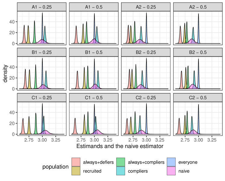
Figure S.1: Distribution of sample causal effect among different populations and estimated naïve difference of mean outcomes across 500 simulated data sets and number of clusters $J\in\{200,500,800\}$ organized by the 12 combinations of scenario, case, and treatment proportion in our configurations.

Figure S.3 shows the true and estimated proportion of always-recruited among the always- and complier-recruited in our simulations, organized by scenario and case. The vertical lines show the (approximate) theoretical values for the true proportion. We see that there is variability around the true proportion from data set to data set, but the estimation procedure is accurate, and it improves as the number of clusters increases.

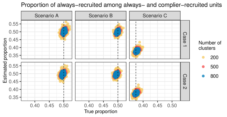
Figure S.2: True sample proportion of always-recruited among the always- and complier recruited units (x-axis) and estimated proportion (y-axis) across 500 data sets and $J\in\{200,500,800\}$ number of clusters (shown in color) organized across the scenario and cases in our simulation configurations. The vertical lines correspond to approximate theoretical values for the true super-population proportion.

Figure S.3: Bias of the causal estimator for the treatment effect among the always-recruited, the complier-recruited, and the recruited populations, across 500 data sets and under 6 scenarios and 3 choices for the number of clusters, when the probability of cluster treatment is 0.25.

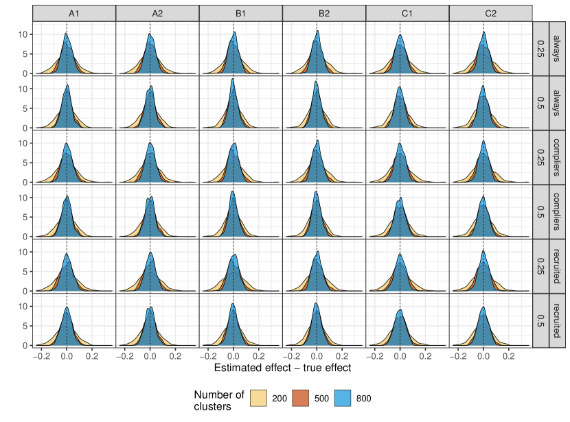
Figure S.4: Bias of the causal estimator that uses the known working propensity score for the treatment effect among the always-recruited, the complier-recruited, and the recruited populations, across 500 data sets and under 6 configurations, 3 choices for the number of clusters, and treatment of clusters set to 0.25 or 0.5.

Figure S.3 shows the estimated minus the true causal effect on the the three populations of interest, the recruited population, the always-recruited and the complier recruited population, when using the proposed estimators with estimated working propensity score and imbalanced designs that assign 25% of the clusters to treatment. These results show that the estimators are essentially unbiased across all scenarios considered. Similarly, Figure S.4 shows the same quantity across all simulation configurations and when using the known working propensity score. As expected, the estimator of the causal effect in the three populations is unbiased, and it is more precise under a larger number of clusters.

Also, Figure S.5 shows the coverage of the 95% confidence intervals for the causal estimators for the effect on the recruited, the always-recruited, the combination of always- and complier-recruited, and the complier-recruited populations. For the estimators that use the known propensity score, we consider 95% intervals based on the derived asymptotic distribution. For the estimators that use the estimated propensity score, we consider a bootstrap procedure that resamples clusters while holding the number of treated clusters fixed, in order to emulate cluster treatment assignment under the simulation design. We calculate the standard deviation of the bootstrap estimates and use them to construct 95% confidence intervals. The coverage of the intervals based on the asymptotic distribution for the estimator that uses the known propensity score is close to 95% across all scenarios. Coverage based on the bootstrap is close to 95% for the estimator of the causal effect on the recruited population, the always-recruited units in the overall population, and the combination of always- and complier-recruited units in the overall population when using the estimated propensity score. Coverage of the same intervals for the causal effect on the compliers are lower, ranging from 85 to 93%, though always closer to the nominal level under Scenario C compared to Scenarios A and B.

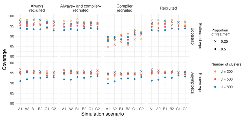
Figure S.5: Coverage of 95% intervals for the estimator of the effect on the recruited, the always-recruited, and the complier-recruited populations, based on the asymptotic distribution for the known working propensity score and the bootstrap for estimated propensity score.

Lastly, we investigate the estimation technique of our working propensity score model parameters. In Figure S.6 we show the distribution of estimated minus true parameter across the simulated data sets for scenario A, case 1, and under different number of clusters. Results from the remaining simulation configurations were similar. We see that the working propensity score estimation technique based on the pseudo-likelihood returns unbiased estimates of the working propensity score parameters, that are closer concentrated near the true value for a larger number of clusters.

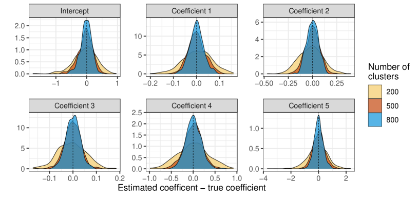
Figure S.6: Distribution of estimated minus true working propensity score coefficients for scenario A, case 1 across simulated data sets, and for different number of clusters.

Appendix D Information on the ARTEMIS trial

Table S.3 provides descriptive information for the enrolled group of patients with treatment (intervention) and without (control). We perform t-tests for continuous covariates and $\chi^{2}$-tests for binary covariates to compare the mean of each covariate in the intervention and control groups. We find that multiple covariates have p-values for the corresponding test that are below 0.05, indicating that the treated and control enrolled groups are different with respect to these characteristics.

Covariate	Intervention	Control	$p$ value
Age (year)	62.0 (11.7)	61.4 (11.5)	0.013
Male (%)	68.9 (46.3)	68.3 (46.5)	0.509
White (%)	90.0 (30.1)	86.4 (34.3)	0.000
Black (%)	8.5 (27.8)	11.3 (31.6)	0.000
College (%)	49.4 (50.0)	53.5 (49.9)	0.000
Private insurance (%)	63.2 (48.2)	65.5 (47.5)	0.018
Prior MI (%)	19.3 (39.5)	21.3 (41.0)	0.015
Prior P2Y12 use (%)	12.6 (33.2)	16.3 (36.9)	0.000
Hemoglobin level	12.87 (2.02)	12.80 (2.08)	0.073
Hypertension (%)	67.2 (47.0)	70.9 (45.4)	0.000
DES use (%)	82.8 (37.8)	78.6 (41.0)	0.000
Diabetes (%)	31.1 (46.3)	34.3 (47.5)	0.000
Employment (%)	48.3 (50.0)	46.9 (49.9)	0.180
Multivessel disease (%)	47.1 (49.9)	45.5 (49.8)	0.133
CABG (%)	1.5 (12.0)	1.4 (11.6)	0.800

Table S.3: Mean Baseline Characteristics of Enrolled Patients by Randomized Arm, with standard deviation in brackets. The $p$-value is computed by $t$-test for continuous data and Pearson’s chi-squared test for binary data.

References

• Angrist et al. [1996] Joshua D Angrist, Guido W Imbens, and Donald B Rubin. Identification of Causal Effects Using Instrumental Variables. Journal of the American Statistical Association, 91(434):444–455, 1996.
• Aronow and Lee [2013] Peter M Aronow and Donald KK Lee. Interval estimation of population means under unknown but bounded probabilities of sample selection. Biometrika, 100(1):235–240, 2013.
• Charnes and Cooper [1962] Abraham Charnes and William W Cooper. Programming with linear fractional functionals. Naval Research logistics quarterly, 9(3-4):181–186, 1962.
• Ding and Lu [2017] Peng Ding and Jiannan Lu. Principal stratification analysis using principal scores. Journal of the Royal Statistical Society: Series B (Statistical Methodology), 79(3):757–777, 2017.
• Ding et al. [2011] Peng Ding, Zhi Geng, Wei Yan, and Xiao-Hua Zhou. Identifiability and estimation of causal effects by principal stratification with outcomes truncated by death. Journal of the American Statistical Association, 106(496):1578–1591, 2011.
• Frangakis and Rubin [2002] Constantine E. Frangakis and Donald B. Rubin. Principal Stratification in Causal Inference. Biometrics, 58(1):21–29, mar 2002. ISSN 0006341X. doi: 10.1111/j.0006-341X.2002.00021.x.
• Frangakis et al. [2002] Constantine E Frangakis, Donald B Rubin, and Xiao Hua Zhou. Clustered Encouragement Designs with Individual Noncompliance: Bayesian Inference with Randomization, and Application to Advance Directive Forms. Biostatistics, 3(2):147–164, 2002.
• Gaebler et al. [2022] Johann Gaebler, William Cai, Guillaume Basse, Ravi Shroff, Sharad Goel, and Jennifer Hill. A causal framework for observational studies of discrimination. Statistics and Public Policy, 9(1):26–48, 2022.
• Hahn et al. [2005] Seokyung Hahn, Suezann Puffer, David J Torgerson, and Judith Watson. Methodological bias in cluster randomised trials. BMC medical research methodology, 5(1):1–8, 2005.
• Jiang et al. [2022] Zhichao Jiang, Shu Yang, and Peng Ding. Multiply robust estimation of causal effects under principal ignorability. Journal of the Royal Statistical Society Series B: Statistical Methodology, 84(4):1423–1445, 2022.
• Jo and Stuart [2009] Booil Jo and Elizabeth A Stuart. On the use of propensity scores in principal causal effect estimation. Statistics in medicine, 28(23):2857–2875, 2009.
• Kahan et al. [2023] Brennan C Kahan, Fan Li, Andrew J Copas, and Michael O Harhay. Estimands in cluster-randomized trials: choosing analyses that answer the right question. International Journal of Epidemiology, 52(1):107–118, 2023.
• Li et al. [2018] F Li, K L Morgan, and A M Zaslavsky. Balancing covariate via propensity score weighting. Journal of the American Statistical Association, 113(521):390–400, 2018.
• Li et al. [2022a] Fan Li, Zizhong Tian, Jennifer Bobb, Georgia Papadogeorgou, and Fan Li. Clarifying selection bias in cluster randomized trials. Clinical Trials, 19(1):33–41, 2022a.
• Li et al. [2022b] Fan Li, Zizhong Tian, Zibo Tian, and Fan Li. A note on identification of causal effects in cluster randomized trials with post-randomization selection bias. Communications in Statistics-Theory and Methods, pages 1–13, 2022b.
• Papadogeorgou et al. [2019] Georgia Papadogeorgou, Fabrizia Mealli, and Corwin M Zigler. Causal inference with interfering units for cluster and population level treatment allocation programs. Biometrics, 75(3):778–787, 2019.
• Papadogeorgou et al. [2022] Georgia Papadogeorgou, Kosuke Imai, Jason Lyall, and Fan Li. Causal inference with spatio-temporal data: estimating the effects of airstrikes on insurgent violence in iraq. Journal of Royal Statistical Society, Series B, 2022.
• Rosenbaum [1984] Paul R Rosenbaum. The Consquences of Adjustment for a Concomitant Variable That Has Been Affected by the Treatment. Journal of the Royal Statistical Society. Series A, 147(5):656–666, 1984.
• Rosenbaum [2002] Paul R. Rosenbaum. Observational studies. Springer, 2002.
• Rosenbaum and Rubin [1983] Paul R Rosenbaum and Donald B Rubin. The central role of the propensity score in observational studies for causal effects. Biometrika, 70(1):41–55, 1983.
• Schochet [2022] Peter Z Schochet. Estimating complier average causal effects for clustered RCTs when the treatment affects the service population. Journal of Causal Inference, 10(1):300–334, 2022.
• Schochet [2023] Peter Z Schochet. Estimating complier average treatment effects for clustered RCTs with recruitment bias. Working paper, 2023.
• Schochet et al. [2022] Peter Z Schochet, Nicole E Pashley, Luke W Miratrix, and Tim Kautz. Design-based ratio estimators and central limit theorems for clustered, blocked rcts. Journal of the American Statistical Association, 117(540):2135–2146, 2022.
• Serfling [2009] Robert J Serfling. Approximation theorems of mathematical statistics, volume 162. John Wiley & Sons, 2009.
• Su and Ding [2021] Fangzhou Su and Peng Ding. Model-assisted analyses of cluster-randomized experiments. Journal of the Royal Statistical Society: Series B (Statistical Methodology), 2021.
• Turner et al. [2017] Elizabeth L. Turner, Fan Li, John A. Gallis, Melanie Prague, and David M. Murray. Review of recent methodological developments in group-randomized trials: part 1–design. American Journal of Public Health, 107(6):907–915, 2017.
• Van der Vaart [2000] Aad W Van der Vaart. Asymptotic statistics, volume 3. Cambridge university press, 2000.
• Wang et al. [2022] Bingkai Wang, Chan Park, Dylan S Small, and Fan Li. Model-robust and efficient inference for cluster-randomized experiments. arXiv preprint arXiv:2210.07324, 2022.
• Wang et al. [2019] Tracy Y. Wang, Lisa A. Kaltenbach, et al., and Eric D. Peterson. Effect of Medication Co-payment Vouchers on P2Y12 Inhibitor Use and Major Adverse Cardiovascular Events among Patients with Myocardial Infarction: The ARTEMIS Randomized Clinical Trial. Journal of the American Medical Association, 321(1):44–55, 2019. ISSN 15383598. doi: 10.1001/jama.2018.19791.
• Zhao et al. [2022] Qingyuan Zhao, Luke J Keele, Dylan S Small, and Marshall M Joffe. A note on post-treatment selection in studying racial discrimination in policing. American Political Science Review, 116(1):337–350, 2022.