Informative path planning for scalar dynamic reconstruction using coregionalized Gaussian processes and a spatiotemporal kernel

Informative path planning for scalar dynamic reconstruction using coregionalized Gaussian processes and a spatiotemporal kernel

Abstract

The proliferation of unmanned vehicles offers many opportunities for solving environmental sampling tasks with applications in resource monitoring and precision agriculture. Informative path planning (IPP) includes a family of methods which offer improvements over traditional surveying techniques for suggesting locations for observation collection. In this work, we present a novel solution to the IPP problem by using a coregionalized Gaussian processes to estimate a dynamic scalar field that varies in space and time. Our method improves previous approaches by using a composite kernel accounting for spatiotemporal correlations and at the same time, can be readily incorporated in existing IPP algorithms. Through extensive simulations, we show that our novel modeling approach leads to more accurate estimations when compared with formerly proposed methods that do not account for the temporal dimension.

I Introduction

Consider the task of modeling a soil property in an agricultural field with a point sensor. Whether the sensor is wielded by a human or an autonomous robot, the agent is tasked with deciding where to capture observations of the environment in order to inform the spatial interpolation. If the environmental properties are dynamic and can change over the course of the survey, the operator is also tasked with the option of updating an old measurement at a previously-visited site, or measuring an unvisited location. When sampling under practical constraints such as time and fuel, the operator must strategically choose sampling locations that allow for useful predictive ability in space and time, in order to arrive at a cohesive estimation of the system’s state at the end of the survey.

Thus, this task of informative path planning (IPP) shares many elements with the task of optimal sensor placement and can be formalized as a constrained optimization, where the agent must evaluate the best location to travel, to satisfy an objective function based in reconstructing a spatial process [23, 3]. Recently, there have been many improvements in approaches to the IPP task for various objectives including: map reconstruction with distributed agents, source position estimation for sound and contaminant plumes, and search and rescue [26].

Figure 1: An overview of our evaluation methodology. (a) shows the ground truth, and the vehicle in the replanning stage, with observation history enumerated. (b) shows the environment during the planning stage with the locations of previous observations. (c) Samples can be visualized along a path in a temporal dimension and (d) displays the final map estimate at all inducing points in the Gaussian process.

Steady efforts have been directed toward sensing strategies for monitoring spatiotemporal processes [7]. The emergence of small, inexpensive mobile platforms points to a future where mobile sensors may be rapidly dispatched to model a dynamic phenomenon. However, to the best of our knowledge there have been limited investigations of informative planners that consider the temporal dimension of information content, especially in an online planning approach. This is necessary to produce faithful representations of dynamic environments, as observations made early in the course of a survey may no longer represent the state of the system at the location at the end of the survey. Additionally, it may be desirable to infer the state of the system at arbitrary points in time, or into the future.

To address this issue, we propose a novel sampling-based IPP framework that considers the information content of sensing locations in space and time. An overview of the framework is shown in Figure 1 and in the accompanying video. Inspired by the asymptotic optimality of IPP methods based on random trees [16] [17] and advancements in large-scale, multiple-output Gaussian process modeling [15], our method combines an information-theoretic sampling-based planner with a spatiotemporal covariance function implemented as a separable kernel to access the information gain from the locations of candidate sensing locations both in space and time. This also allows for both inference of the state and inference of model uncertainty for unexplored parts of the system and establishes a criterion for revisiting already-observed locations that no longer meaningfully reduce uncertainty of the system’s current state.

The contributions of this work are:

• A framework for reasoning about the information content of observations in arbitrary dimensions reconciled to a metric appropriate for path planning

• The integration of this spatiotemporal information function in a novel time-aware informative planner for terrestrial monitoring

• Validation of the approach in the context of spatial and temporal priors with simulated and real-world dynamic scenarios inspired by common environmental dispersion processes

• Exploration of interactions between the parameters governing the planner and the model

Our work opens up several avenues for consideration: the continuous update of spatial and temporal priors through adaptive planning, extensions into multi-robot systems, combined sensing modalities for prediction in multiple dimensions (in a manner similar to Co-Kriging in the geostatistical literature), and extensions into different classes of multi-output Gaussian processes. Our framework will be open-sourced, for use in future investigations.

This paper is organized as follows: Selected related work is presented in section II. The problem formulation is introduced in section III and our methods are discussed in section IV. In section V we experimentally evaluate our proposal and conclude in section VI.

II Related Work

This paper draws from a rich body of literature, surrounding the task of collecting observations by an autonomous agent for modeling the distribution of a variable of interest in the environment. IPP approaches have been extended to encompass different sensing modalities (e.g. altitude-dependent sensor models [26]). Notably, most IPP approaches consider the spatial phenomenon to be static or at steady-state, or they assume that the phenomenon does not change meaningfully during the duration of the survey.

IPP for robotic planning is similar to methods which seek to optimize the placement or visitation of environmental sensors [21]. IPP problems that employ an adaptive planning approach re-compute vehicle trajectories as observations are collected. This approach can be framed under the category of problems which involve sequential decision-making with uncertainty, which in turn can be formally described as a Partially-observable Markov Decision Process (POMDP) [18]. As a constrained optimization problem, IPP shares may qualities with the orienteering problem [8].

Other methods leverage optimization techniques to determine the most informative route through a collection of candidate actions or locations. These approaches include Bayesian optimization [2], evolutionary algorithms [25], and reinforcement learning [27].

The asymptotic optimality of rapidly-exploring random trees (RRT) has been leveraged to solve IPP tasks in a computationally tractable manner, including exploration applications where the robot is tasked with monitoring an unknown parameter of interest [19]. Rapidly-exploring information gathering (RIG) algorithms approach the IPP task using incremental sampling with branch and bound optimization [16]. Our work builds on [17], which extended RIG with an information-theoretic utility function and a related stopping criterion.

III Problem Formulation

In this work, we consider the problem of reconstructing a dynamic scalar field given a limited number of observations, collected along a path. Paths are generated using a receding-horizon approach, alternating between planning and execution of the plan until the traveled distance exceeds the budget $B$ or a prediction window $t_{max}$. The task can be formulated as a constrained optimization problem, where information quantity is to be maximized subject to an observation cost. In [16], the task is specified follows:

$$\mathcal{P}^{*}=\underset{\mathcal{P}\in\Psi}{\textnormal{argmax\ }}I(\mathcal{P})\ \textrm{s.t.}\ c(\mathcal{P})\leq B$$ (1)

where $\mathcal{P}^{*}$ is an optimal trajectory found in the space of possible trajectories $\Psi$, for an individual or set of mobile agents such that the cost of executing the trajectory $c(\mathcal{P})$ does not exceed an assigned motion budget, $B$. $I(\mathcal{P})$ is the information gathered along the trajectory $\mathcal{P}$, and the movement budget can be any cost that constrains the effort used to collect observations (e.g., fuel, distance, time, etc.)

This paper inherits the assumptions of the original RIG formulation and of prior sampling-based motion planning literature [16], [19] and adds the following assumptions with respect to time:

1. The state of the robots and the environment are modeled using discrete time dynamics

2. Movement of the sampling agent is anisotropic in the time dimension (see: section V)

To quantify the information content of a trajectory, we employ a utility function that optimizes for a reduction in the posterior variance of the GP used to model the environment. This follows from framing the information gain of an observation as a reduction of map entropy or uncertainty. In [5], the authors present an approach for quantifying the information content of a map $M$ as its entropy $H$ and the information content of a new observation $Z$ as the mutual information between $M$ and $Z$, denoted as $I(M;Z)$ and defined as follows:

$$I(M;Z)=H(M)-H(M\mid Z)$$ (2)

We take advantage of the submodularity of mutual information; that is, the information gained by adding an observation to a smaller set is more useful than adding the same observation to a larger (super-) set (See [22] for an analysis of the benefit of submodular information functions for informative sensing applications and [14] for the submodularity of mutual information.)

From the perspective of the environmental modeling task, a useful survey is one that produces the most accurate representation of the environment, minimizing the expected error given field observations. This follows from equations (1) and (2). This assumption holds when the model is well-calibrated with respect to the priors embodied in the model parameters . Our approach can be extended to an adaptive planning scenario, where model hyperparameters are updated based on new measurements and future path plans leverage the updated model. In previous work, we have demonstrated how model priors can encode modeler intuition, resulting in sampling strategies that vary in the degree if exploration [4].

IV Methods

IV-A Environmental Model

We describe the spatial distribution of an unknown stochastic, dynamic environmental process occurring in a region $\xi\subset\mathbb{R}^{2}$ as a function $f\colon\mathcal{X}\to\mathbb{R}$ that is sampled and modeled at the discrete grid, $\mathcal{X}\subset\mathbb{R}^{N_{t}\times N_{x,y}}$. Here $N_{x,y}$ is a discretization of the spatial domain $\xi$, while $N_{t}$ is the temporal domain in which the spatial process evolves.

The environmental map comprises this function $f$ that describes our observations $y_{i}$, plus some additive measurement noise $\varepsilon_{i}$, i.e., $y_{i}=f(x_{i})+\varepsilon_{i}$, where we assume that this noise follows an i.i.d. Gaussian distribution with zero mean and variance $\sigma_{n}^{2}$: $\varepsilon\sim\mathcal{N}\left(0,\sigma_{n}^{2}\right)$. We assume that $f$ is a realization of a Gaussian process, represented as a probability distribution over a space of functions. Through marginalization, we can obtain the conditional density $f\mid y=\mathcal{N}(\mu_{f\mid y},\Sigma_{f\mid y})$. The joint distribution of observations $\mathbf{y}$, $\{f(x_{1})+\varepsilon_{1},\dots,f(x_{n})+\varepsilon_{n}\}$ and predictions $\mathbf{f}$, $\{f_{\star},\dots,f_{\star^{n}}\}$ at indices $\mathbf{X_{i},t}$, $\{x^{(st)}_{1,1},\dots,x^{(st)}_{m,n}\}$ becomes:

$$\small\begin{bmatrix}\mathbf{y}\\ f(x_{\star})\\ \end{bmatrix}\sim\mathcal{N}\left(0,\begin{bmatrix}[cc]k(\mathbf{X},\mathbf{X})+\sigma^{2}I_{N}&k\left(\mathbf{X},x_{\star}\right)\\ k\left(x_{\star},\mathbf{X}\right)&k\left(x_{\star},x_{\star}\right)\end{bmatrix}\right)$$ (3)

where s and t denote spatial and temporal indices respectively. Here, environmental observations $y$, are drawn from a training set $\mathcal{D}$ of $n$ observations, $\mathcal{D}=(X,\mathbf{y})=\left\{\left(\mathbf{x}_{i,t},y_{i,t}\right)\mid i=1,\ldots,n\right\}$. $k$ is the covariance function (or kernel), $\sigma^{2}_{n}$ is the variance of the observation noise, and input vectors $\mathbf{x}$ and query points $\mathbf{x_{\star}}$ of dimension $D$, are aggregated in the $D\times n$ design matrices $X$ and $X_{\star}$ respectively. From the Gaussian process, we can obtain estimations of both the expected value of the environmental field and the variance of each prediction. Noteworthy is the posterior variance, which takes the form:

$$\sigma=\mathbb{V}\left[f_{\star}\right] =k\left(x_{\star},x_{\star}\right)-k\left(x_{\star},\mathbf{X}\right)\times$$ (4)

$$\quad\left[k(\mathbf{X},\mathbf{X})+\sigma_{n}^{2}\mathbf{I}_{n}\right]^{-1}k\left(\mathbf{X},\mathbf{x}_{*}\right)$$

The differential entropy of a Gaussian random variable is a monotonic function of its variance, and can be used to derive the information content of a proposed measurement. We will show how this can be used to approximate information gain (equation (2)) in subsection IV-D.

It is important to note that for fixed kernels the variance does not depend on the value of the observation, allowing us to reason about the effectiveness of a proposed observation before traveling to the sampling location [23]. Also notable is the kernel k which establishes a prior over the covariance of any pair of observations. Separate priors can be established in spatial or temporal dimensions, leading to the opportunity to incorporate spatial and/or temporal domain knowledge into the planning process.

IV-B Spatiotemporal prior

The modeling effort can be framed as a multi-task (or multi-output) prediction of correlated temporal processes at each spatial discretization $N_{x,y}$. As we only have a finite set of sampling vehicles (one, in fact), we cannot observe all of the spatial "outputs" for a given time, however we can establish a basis upon which they can be correlated [12]. Specifically, the Linear Model of Coregionalization (LMC) has been applied to GP regression where p outputs are expressed as linear combinations of independent random vector-valued functions $f:\mathcal{T}\rightarrow\mathbb{R}^{p}$. If these input functions are GPs, it follows that the resulting model will also be a GP [1]. The multi-output GP (MOGP) can be described by a vector-valued mean function and a matrix-valued covariance function (see Equation (4)). A practical limitation of MOGPs has been their computational complexity. For making $p$ predictions with $n$ input observations $y\left(t_{1}\right),\ldots,y\left(t_{n}\right)\in\mathbb{R}^{p}$, the complexity of inference is $\mathcal{O}\left(n^{3}p^{3}\right)$ in time and $\mathcal{O}\left(n^{2}p^{2}\right)$ in memory [6]. A variety of strategies exist to solve lighter, equivalent inference tasks under simplifying assumptions, such as expressing an output from linear combinations of latent functions that share the same covariance function, but are sampled independently [1]. Since our information function is only dependent on the posterior covariance, we can take advantage fast approximations with complexity $\mathcal{O}(k(n+p\log p)$ (see discussion in subsection IV-D).

As mentioned earlier, the kernel $k$ establishes a prior likelihood over the space of functions that can fit observed data in the regression task. For the regression of discretely-indexed spatiotemporal data, where space is indexed by $s$ (eg. latitude/longitude) and time is indexed by $t$ (eg. seconds), we build a composite kernel by multiplying a spatial and temporal kernel:

$$k((s,t),t(s^{\prime},t^{\prime}))=k_{s}(s,s^{\prime})k_{t}(t,t^{\prime})$$ (5)

While other approaches to kernel composition are possible and encode different environmental priors, constructing a kernel that is separable along input dimensions affords considerable computational advantages. More generally, when $k(\mathbf{x},\mathbf{x}^{\prime})=\prod_{d=1}^{D}k^{(d)}(\mathbf{x}^{(d)},\mathbf{x}^{\prime(d)})$, the kernel (Gram) matrix $K$ can be decomposed into smaller matrices $K=K_{1}\otimes\cdots\otimes K_{D}$ which can be computed in $\mathcal{O}(Dn^{\frac{D+1}{D}})$ time (see [31] and [9] for more on kernel composition for multidimensional regression.)

For the spatial relation, we use the Matérn kernel with $\nu=3/2$ and fixed hyperparameters. Comprehensively described in [29], the Matérn kernel is a finitely-differentiable function with broad use in the geostatistical literature for modeling physical processes due in part to its ability to resist over-smoothing natural phenomena with sharp discontinuities. It takes the form:

$$K_{\text{Matern}}(X,X_{\star})=\sigma^{2}\frac{2^{1-\nu}}{\Gamma(\nu)}\left(\frac{\sqrt{2v}}{l}r\right)^{\nu}K_{\nu}\left(\frac{\sqrt{2\nu}}{l}r\right)$$ (6)

where $K_{\nu}$ is a modified Bessel function , $\Gamma(\cdot)$ is the Gamma function, and $r$ is the Euclidean distance between input points $X$ and $X_{\star}$. $\nu>0$, $l>0$, and $\sigma^{2}>0$ are hyperparemeters representing smoothness, lengthscale, and observation variance respectively. We use a radial basis function kernel (RBF or squared-exponential) in the time dimension to smoothly capture diffusive properties that may fade in time. Note that the Matérn kernel approaches the RBF as $\nu\to\infty$.

IV-C Informative Planning

In this work, we present a novel planner IIG-ST to address IPP task defined in equation (1). Our planner is built upon IIG-Tree, a sampling-based planner with an information-theoretic utility function and convergence criterion [17] and derived from the family of Rapidly-exploring Information Gathering (RIG) algorithms introduced by Hollinger and Sukhatme [16]. RIG inherits the asymptotic cost-optimality of the $\mathrm{RRT}^{\star}$, $\mathrm{RRG}$, and $\mathrm{PRM}^{\star}$ algorithms [20], a conservative pruning strategy from the branch and bound technique [3], and an information-theoretic convergence criterion (see discussion in subsection IV-E). We add routines to consider the time dimension of samples in the tree and combine it with a hybrid covariance function and stopping criterion grounded in map accuracy.

IV-D Information Functions

From equation (2), we established information gain as the reduction of map entropy $H$ given a new observation $Z$.

If the map is modeled as a Gaussian Process where each map point (or query point) is a Gaussian random variable, we can approximate mutual entropy with differential entropy. For a Gaussian random vector of dimension $n$, the differential entropy can be derived as $h(X)=\frac{1}{2}\log\left((2\pi e)^{n}|\Sigma|\right)$. If we let $X\sim\mathcal{N}\left(\mu_{X},\Sigma_{X}\right)$ and $X\mid Z\sim\mathcal{N}\left(\mu_{X\mid Z},\Sigma_{X\mid Z}\right)$ be the prior and posterior distribution of the random vector $X$, before and after incorporating observation $Z$, then the mutual information becomes:

$$I(X;Z)=\frac{1}{2}\left[\log\left(|\Sigma_{X}|\right)-\log\left(|\Sigma_{X\mid Z}|\right)\right]$$ (7)

where $\Sigma$ is the full covariance matrix.

For a random vector $\mathbf{X}=(X_{1},\ldots,X_{n})$ with covariance matrix K, the mutual information between $\mathbf{X}$ and observations Z can be approximated from equation (7) as:

$$\hat{I}(X;Z)=\sum_{i=1}^{n}\frac{1}{2}\left[\log\left(\sigma_{X_{i}}\right)-\log\left(\sigma_{X_{i}\mid Z}\right)\right]$$ (8)

Using marginalization, for every $X_{i}$, it holds that $\mathbb{V}\left[X_{i}\right]=K^{[i,i]}$. The expression becomes:

$$\hat{I}^{[i]}\left(X_{i};Z\right)=\frac{1}{2}\left[\log\left(\sigma_{X_{i}}\right)-\log\left(\sigma_{X_{i}\mid Z}\right)\right]$$ (9)

and can be computed as the sum of marginal variances at i: $\hat{I}(X;Z)=\sum_{i=1}^{n}\hat{I}^{[i]}(X_{i};Z)$ (see [17] for a derivation).

The main motivation of using marginal variances at evaluation points (Equation (8)) is to avoid maintaining and updating (inverting) the full covariance matrix. This is of a particular concern for spatiotemporal modeling, because the number of inducing points grows on the order of $m\times n$ for a spatial domain of $m$ rows and $n$ columns. Alternate GP formulations such as spatio-temporational sparse variational GPs (ST-SVGP) allow for computational scaling that is linear in the number of time steps [15] For computing the posterior variance at GP inducing points, we use LOVE (LanczOs Variance Estimates), for a fast, constant-time approximation of predictive variance [24, 11].

Algorithm 1 Information_GPVR-ST()

1: 2:Proposed robot pose or location from RRT/RIG Steer $p$, current map/state estimate $\mathcal{M}_{\mathcal{D}}$, covariance function $k(\cdot,\cdot)$, prior map variance $\sigma$, variance of observation noise $\sigma_{n}^{2}$, near node information $I_{\text{near}}$;

3: $\bar{\sigma}\leftarrow\sigma$ $\triangleright$ Initialize updated map variance as the current map variance

4: if $I_{\text{near }}$ is not empty then $\triangleright$ Initialize information gain

5:      $I\leftarrow I_{\text{near }}$

6: else

7:      $I\leftarrow 0$

8: $z\leftarrow$ Propose a future measurement at location $p$ and map $\mathcal{M}$ $\triangleright$ Calculate posterior map variance at training and query points

9: $\bar{\sigma}\leftarrow\texttt{LOVE}\left(X,X_{*}\right)$

10: for all $i\in\mathcal{M}_{\mathcal{D}}$ do

11:      $I\leftarrow I+1/2\left[\operatorname{logdet}\left(\sigma^{[i]}\right)-\operatorname{logdet}\left(\bar{\sigma}^{[i]}\right)\right]$

12: return $I$ (total information gain), $\bar{\sigma}$ (updated map variance)

Algorithm 1 details the procedure for updating a node’s information content. In lines 6-8, the location of a future measurement $z$ at pose $p$, is added to the set of past observations (training points) from the entire node graph. This is used to create a new map state containing the previous training points plus the new measurement and the preexisting query points where the GP is evaluated. Next, the posterior variance is calculated (lines 8) using LOVE (LanczOs Variance Estimates) [24, 11] to produce a posterior variance at the proposed locations of training points $X\in\mathcal{M}_{\mathcal{D}}$, query points $X_{*}\in\mathcal{M}_{\mathcal{D}}$, and the variance of observation noise $\sigma_{n}^{2}$. Finally, information content of the entire posterior map is updated and the information gain is returned as a marginal variance (lines 9-11).

IV-E Convergence criterion

The closely related Incrementally-exploring Information Gathering (IIG) algorithm modifies RIG with an information-theoretic convergence criterion [17]. Specifically, IIG bases the stopping criterion around a relative information contribution (RIC) criterion that describes the marginal information gain of adding a new observation relative to the previous state the RIG tree (see Equation 15 in [17] for a comprehensive discussion of the IIG algorithm and for a definition of the RIC). There, it was used as a tunable parameter that established a planning horizon for information gathering. In this paper, we use posterior map variance as a lower bound for mean-square error (MSE) (Equation (10)) at a arbitrary test location in the GP, given optimal hyperparameters $\theta$ for the GP regression model. We replace the stopping criterion in IIG with a threshold established by the operator as the lower bound of expected prediction MSE.

$$\operatorname{MSE}\left(\widehat{f_{\star}}\right)\geq\underbrace{\mathbb{V}\left[f_{\star}\right]}_{=\sigma_{\star\mid y}^{2}(\theta)}$$ (10)

It is important to note that this inequality holds for the hyperparameters $\theta$ that produce an optimal predictor of $f$ (see Result 1 in [30] for a proof of Equation (10) using the Bayesian Cramér-Rao Bound (BCRB).) In practice, $\theta$ is learned from the data. For approximate (suboptimal) values of $\theta$, the bound of Equation (10) will not hold, as additional error is introduced from the unknown model hyperparameters. However, when coupled with adaptive planning techniques to learn $\theta$ from observations, then the posterior variance approaches the true lower bound of the MSE. A deeper analysis of the implications of this application is a target of future work.

IV-F Path selection and planning

Once the planner terminates (either by the convergence criterion or after a fixed planning horizon), a path must be selected from the graph of possible sampling locations. We use a vote-based heuristic from [17] that ranks paths according to a similarity ratio and biases towards paths that are longer and more informative with a depth-first search. In the simulated environment, parameters are set for vehicle speed, sampling frequency, and replanning interval. The vehicle alternates between planning, executing, and replanning in a receeding-horizon fashion, such that 2-3 waypoints are visited in each planning interval.

The path selection strategy is independent of the informative path planning algorithm and can be thought of as an orienteering problem within a tree of sampling locations.

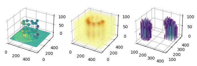
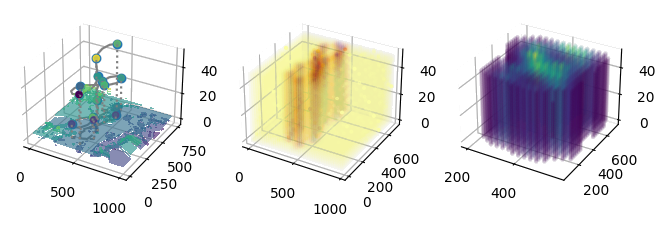
Figure 2: A visualization of the benchmark (coverage) sampling scenarios (top: fluid simulation, bottom: ocean sampling simulation). The posterior variance is depicted in the second panel, and the posterior mean in the third, with near-zero values filtered show the underlying structure. The coverage planners are given a path budget and node budget equivalent to the median of the equivalent metrics among all runs of the informed planners. Observations are collected on a circlular coverage in the synthetic environment and a lemniscatic coverage in the oceanic experiment.

V Experimental Evaluation and Discussion

In this section, we contrast our proposed spatiotemporal-informed planner (IIG-ST) against a traditional coverage survey strategy (see Figure 2), and an informed planner that does not consider temporal variation (IIG). We evaluate the accuracy of the final map representation at the end of the survey period under varying choices of spatial and temporal priors. We also consider the ancillary objective of making predictions of the state of environment at arbitrary points in time. This can be useful for objectives that wish to reconstruct the dynamics of a system, such as modeling a vector field. However, this is complicated by the fact that the survey envelope is anisotropic in the temporal dimension – the robot and sensor can only travel forward through time.

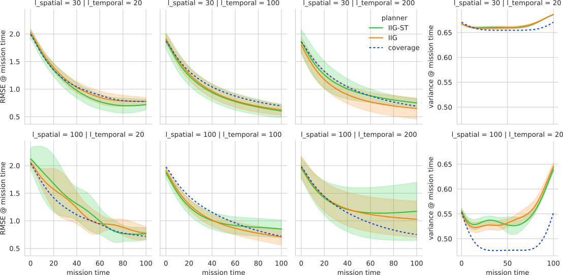
Figure 3: [Advection/diffusion simulation] A comparison of map error and posterior variance (lower is better) at different locations in the mission time for different spatiotemporal priors Optimal priors are chosen in the top left panel ($\ell_{t}=20$ and $\ell_{s}=30$) and become increasingly suboptimal in other panels. IIG-ST (our planner) is compared the same planner lacking time information (IIG) and a circular survey strategy. The error metric is expressed across the entire spatial domain at different time indices (denoted on the x-axis), and reflects the error between the estimated map and the state of the environment at that time. Y-axis scales are shared between rows.

V-A Experimental setting

Our objective is to model the end-state of a spatial phenomenon that undergoes advection and diffusion in a 2D environment. This can represent the movement of a substance of interest in a fluid, a porous medium such as soil, or any number of similar natural processes. Two fluid parcels are initialized with inversely-proportional velocities, at opposite corners of a $500\times 500$-unit gridded environment. The fluid parcels advect and diffuse according to the Navier-Stokes equations for an incompressible fluid, implemented as a forward-differencing discretization without boundary conditions.

We initialized the RIG-planner with fixed planning parameters: the vehicle can move a maximum of 100 map-units, every 5 time-units. Replanning is done every 10 time increments, and planning within each increment stops when estimated $\mathbb{V}\left[f_{\star}\right]=0.15$. Sampling occurs once every 5 time increments. We set the time budget to be 100 units and compute the accuracy of the final representation of the map at $t=50$ min. Map accuracy at different moments in mission time are presented in Figure 3. While the planner was not given a movement budget, the fixed speed of the vehicle and finite time-horizon resulted in consistent numbers of observations $(M=21.0,SD=0.2)$ and path lengths $(M=1236,SD=36)$ among the informative planners. The coverage baseline is given a proportional budget (21 observations, 1610 map units traveled). This is sufficient to complete a full tour of the environment with revisitation (see Figure 2). The full table of parameters set for the planner can be found in the accompanying video. We executed the experiments in a GNU/Linux environment on a 3.6 GHz Intel i7-4790 computer with 11 GB of RAM available. All procedures used single-threaded Python implementations for RRT sampling from [28] and multi-threaded posterior variance final map predictions were performed using implementations from GPyTorch [11] without GPU or TPU acceleration so as to simulate the resources available on an embedded system.

V-B Consequences of the temporal prior

To demonstrate the consequences of incorporating a spatiotemporal prior on informative planning in dynamic fields, we use the composite covariance function given in equation (5) both in planning and for evaluating the accuracy of the final map representation. This is notable for the baseline comparisons–while the coverage planner follows a deterministic trajectory, different map accuracies and variance reductions are expected depending on the choice of spatiotemporal prior during the construction of the final map model.

For the temporal relation, we use a RBF kernel with length scales of $\ell_{t}=20,100,200$ time units. The spatial relation comprises a Matérn kernel with $\nu=3/2$ and length scales of $\ell_{s}=100$ distance units. To verify that the robot solves the problem in section III, we evaluate the root-mean squared error between the map representation at $t=100$ and the state of the field at the same time. As the planner only requires the posterior covariance, it is not necessary to produce continuous estimations of the map state, so the final representation is computed once the simulation has ended. 20 episodes are run for each hyperparameter combination and summaries of average error, average posterior variance and standard deviations are found in table I.

			RMSE		$\overline{V}$
planner	$\ell_{s}$	$\ell_{t}$	$t_{max}$	$t_{all}$	$t_{max}$	$t_{all}$
IIG	30	20	0.781 (0.066)	1.123 (0.072)	0.686 (0.0)	0.664 (0.001)
		100	0.612 (0.096)	1.035 (0.098)	0.64 (0.005)	0.626 (0.006)
	100	20	0.762 (0.113)	1.288 (0.179)	0.645 (0.007)	0.547 (0.004)
		100	0.75 (0.222)	1.093 (0.116)	0.462 (0.02)	0.413 (0.025)
IIG-ST	30	20	0.733 (0.089)	1.092 (0.064)	0.686 (0.0)	0.665 (0.001)
		100	0.611 (0.121)	1.028 (0.135)	0.638 (0.005)	0.624 (0.006)
	100	20	0.768 (0.101)	1.3 (0.238)	0.64 (0.004)	0.547 (0.005)
		100	0.866 (0.194)	1.114 (0.117)	0.458 (0.014)	0.414 (0.017)
coverage	30	20	0.777	1.132	0.671	0.658
		100	0.697	1.099	0.639	0.638
	100	20	0.718	1.173	0.552	0.491
		100	0.721	1.19	0.398	0.394

		RMSE
planner	$\ell_{s}$	$t_{max}$	$t_{all}$
IIG	5	6.654 (0.015)	5.499 (0.004)
	40	5.934 (0.382)	4.926 (0.087)
	100	3.835 (0.725)	3.777 (0.17)
IIG-ST	5	6.658 (0.013)	5.499 (0.003)
	40	5.846 (0.305)	4.904 (0.072)
	100	4.1 (0.739)	3.698 (0.252)
coverage	5	3.826	6.238
	40	3.281	5.506
	100	2.909	4.56

TABLE I: (L) [Advection/diffusion] Aggregated ($n=20$) map accuracy (RMSE) and posterior variance (mean, std) of the spatiotemporal planner (IIG-ST) compared to a spatial-only and deterministic survey strategies for fixed length scales. (R) [Ocean dataset] Aggregated $n=20$ map accuracy for the ocean water quality experiment ($\ell_{t}=100$ for all runs). Lower numbers are better. Note: standard deviation values are not expressed for the deterministic planner.

In Figure 3, we examine the choice of kernel hyperparameters on the performance of our planner. Optimal parameters were established offline using the baseline samples and a standard marginal log likelihood function and the Adam optimizer in gpytorch ($\ell_{t}=20$ and $\ell_{s}=30$). These serve as the basis of comparison in the top-left panel of Figure 3 and resulted the spatiotemporal planner outperforming the temporally-naive and baseline planner for on average, throughout the entire mission duration. Large lengthscales imply a greater degree of correlation across space or time, and result a greater reduction of posterior variance. A reduction of model uncertainty should translate to a higher map accuracy, however this is not the case if the spatial priors are unrepresentative. For example, while the coverage planner had lower variance due to a longer path traveled and more dispersed observations, the resulting map accuracy was not better than the informative planners, leading to the conclusion that the spatiotemporal prior did not reflect the variation of the observed process. We want to emphasize that path planning algorithms based around variance reduction should also place the metric within a broader context of the practical objective – map accuracy.

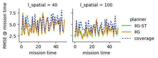
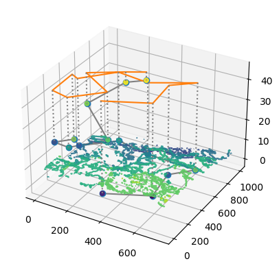
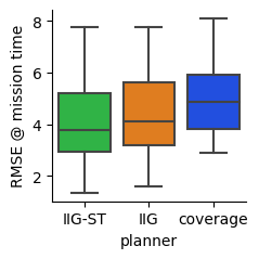
Figure 4: Example results from the ocean modeling experiments. (Top) Map error as a function of mission time, ($\ell_{t}=100$). (L) Example trajectory, with path trace projected above a representation of the environment at $t=0$. (R) Aggregated statistics from the figures in the top panel.

For informative planners, the effect is magnified, as the planner will move toward more dispersive sampling, thus missing high-frequency spatial phenomena entirely. This is demonstrated in the marginally improved accuracy and lower posterior variance for IIG-ST when given a unrepresentative spatial and temporal prior. In worst-case scenarios, a very unrepresentative temporal prior ($\ell_{t}=200$) can reduce the performance of the spatiotemporal planner below the baseline (Figure 3, Col. 2). As the ultimate goal of informed robotic sensing is model accuracy and not simply variance reduction, hyperparameter optimization must be a key component for accurate mapping and is a common practice in adaptive planning [10]. Furthermore, a time-varying kernel could be specified and optimized as observations of the environment are gathered. Future work will investigate the effect and performance of updating model priors during the course of a survey mission.

The final map posterior is evaluated with the same spatiotemporal kernel in all cases, regardless of planning method to ensure a fair comparison between the methods. Only the spatiotemporal planner (IIG-ST) is able to make use of temporal variance during replanning. Training observations are obtained from a point sensor model, where the a "sample" is obtained by the simulated agent querying the ground-truth scalar field at a sample location. We use a sparse representation of posterior variance, evaluated at a 1/20 scale spatial resolution for a total of $25\times 25\times 50$ query (inducing) points. Recent advancements in spatiotemporal GPs with separable kernels, enable computational scaling to scale lineally in the temporal dimension, instead of cubic [15]. These and other recent developments are reducing the computational burden of large GPs and informative planning with spatiotemporal information at a large scale.

V-C Ocean particulate mapping scenario

We demonstrate our spatiotemporal IPP approach in a syoptic-scale simulation using real-world ocean reflectance data. The data was collected in an approximately 1500 x 1000 km region off the west coast of California from the Moderate Resolution Imaging Spectroradiometer (MODIS) aboard NASA’s Terra and Aqua earth observation satellites [13]. Rasters of weekly median reflectance from band 9 (443 nm wavelength) were assembled for the calendar year of 2020. Backscattered light in this wavelength band is highly correlated with the concentration of suspended organic and inorganic particles (e.g. sediments) in the water. In terrestrial and oceanic waters, this can be used as an indicator of water quality, which can guide management decisions related to water diversion and treatment.

We simulated an autonomous aquatic vehicle (AUV) with characteristics similar to the Wave Glider, which is an AUV capable of extended oceanic monitoring campaigns by using oceanic waves for propulsion. Based on the long-mission average speed of 1.5 knots, our simulated vehicle could cover a maximum of 330 km per week. We compare the performance of our informed planner against a fixed lemniscatic coverage pattern. As with the previous section, we evaluate the RMSE of the map representation, both at the final time step and at arbitrary temporal increments in the mission envelope. Summaries of average error, standard deviations, and posterior variance are presented in Table I and Figure 4. As with the previous experiment, posterior variance and map accuracy are evaluated at a 1/20 scale spatial resolution. Also, as with the previous experiment, the performance of IIG-ST is sensitive to the choice of hyperparameters.

VI Conclusion

This work presented an approach for environmental modeling using a novel spatiotemporally-informed path planner. We presented a framework for quantifying the information gain of sampling locations based on their location and time and quantifying the operative outcome – map accuracy. We show that this informed strategy is computationally tractable with modern computational techniques and can outperform naive and conventional approaches, conditional on an appropriate spatiotemporal prior. Multiple avenues for future work lead from this effort. Adaptive planning can be used to revise the spatiotemporal prior as measurements are collected between replanning intervals. This approach can be extended to consider time-varying kernels. variable sensor models, and multi-robot systems.

References

- [1] Mauricio A. Álvarez and Neil D. Lawrence. Computationally Efficient Convolved Multiple Output Gaussian Processes. Journal of Machine Learning Research, 12(41):1459–1500, 2011.
- [2] Shi Bai, Jinkun Wang, Fanfei Chen, and Brendan Englot. Information-theoretic exploration with Bayesian optimization. In 2016 IEEE/RSJ International Conference on Intelligent Robots and Systems (IROS), pages 1816–1822, October 2016.
- [3] J. Binney and G. S. Sukhatme. Branch and bound for informative path planning. In 2012 IEEE International Conference on Robotics and Automation, pages 2147–2154, May 2012.
- [4] Lorenzo Booth and Stefano Carpin. Distributed estimation of scalar fields with implicit coordination. In Distributed Autonomous Robotic Systems, Springer Proceedings in Advanced Robotics, Monbellard, FR, 2023. Springer International Publishing.
- [5] F. Bourgault, A. A. Makarenko, S. B. Williams, B. Grocholsky, and H. F. Durrant-Whyte. Information based adaptive robotic exploration. In IEEE/RSJ International Conference on Intelligent Robots and Systems, volume 1, pages 540–545 vol.1, September 2002.
- [6] Wessel Bruinsma, Eric Perim, William Tebbutt, Scott Hosking, Arno Solin, and Richard Turner. Scalable Exact Inference in Multi-Output Gaussian Processes. In Proceedings of the 37th International Conference on Machine Learning, pages 1190–1201. PMLR, November 2020.
- [7] Jeffrey A. Caley and Geoffrey A. Hollinger. Data-driven comparison of spatio-temporal monitoring techniques. In OCEANS 2015 - MTS/IEEE Washington, pages 1–7, October 2015.
- [8] Stefano Carpin and Thomas C. Thayer. Solving Stochastic Orienteering Problems with Chance Constraints Using Monte Carlo Tree Search. In 2022 IEEE 18th International Conference on Automation Science and Engineering (CASE), pages 1170–1177, August 2022.
- [9] Seth R Flaxman. Machine Learning in Space and Time. PhD thesis, Carnegie Mellon University, Pittsburgh, PA, August 2015.
- [10] Jan N. Fuhg, Amélie Fau, and Udo Nackenhorst. State-of-the-Art and Comparative Review of Adaptive Sampling Methods for Kriging. Archives of Computational Methods in Engineering, 28(4):2689–2747, June 2021.
- [11] Jacob R. Gardner, Geoff Pleiss, David Bindel, Kilian Q. Weinberger, and Andrew Gordon Wilson. GPyTorch: Blackbox matrix-matrix Gaussian process inference with GPU acceleration. In Proceedings of the 32nd International Conference on Neural Information Processing Systems, NIPS’18, pages 7587–7597, Red Hook, NY, USA, December 2018. Curran Associates Inc.
- [12] Pierre Goovaerts and Department of Civil and Environmental Engineering Pierre Goovaerts. Geostatistics for Natural Resources Evaluation. Oxford University Press, 1997.
- [13] NASA Ocean Biology Processing Group. MODIS-Aqua Level 3 Mapped Particulate Organic Carbon Data Version R2018.0, 2017.
- [14] Carlos Guestrin, Andreas Krause, and Ajit Paul Singh. Near-optimal sensor placements in Gaussian processes. In Proceedings of the 22nd International Conference on Machine Learning - ICML ’05, pages 265–272, Bonn, Germany, 2005. ACM Press.
- [15] Oliver Hamelijnck, William J. Wilkinson, Niki Andreas Loppi, Arno Solin, and Theo Damoulas. Spatio-Temporal Variational Gaussian Processes. In Advances in Neural Information Processing Systems, November 2021.
- [16] Geoffrey A. Hollinger and Gaurav S. Sukhatme. Sampling-based robotic information gathering algorithms. The International Journal of Robotics Research, 33(9):1271–1287, August 2014.
- [17] Maani Ghaffari Jadidi, Jaime Valls Miro, and Gamini Dissanayake. Sampling-based incremental information gathering with applications to robotic exploration and environmental monitoring:. The International Journal of Robotics Research, 38(6):658–685, April 2019.
- [18] Leslie Pack Kaelbling, Michael L. Littman, and Anthony R. Cassandra. Planning and acting in partially observable stochastic domains. Artificial Intelligence, 101(1-2):99–134, May 1998.
- [19] Sertac Karaman and Emilio Frazzoli. Incremental Sampling-Based Algorithms for Optimal Motion Planning, May 2010.
- [20] Sertac Karaman and Emilio Frazzoli. Sampling-based algorithms for optimal motion planning. The International Journal of Robotics Research, 30(7):846–894, June 2011.
- [21] A. Krause, C. Guestrin, A. Gupta, and J. Kleinberg. Near-optimal sensor placements: Maximizing information while minimizing communication cost. In 2006 5th International Conference on Information Processing in Sensor Networks, pages 2–10, April 2006.
- [22] Andreas Krause and Carlos Guestrin. Submodularity and its applications in optimized information gathering. ACM Transactions on Intelligent Systems and Technology (TIST), July 2011.
- [23] Andreas Krause, Ajit Singh, and Carlos Guestrin. Near-Optimal Sensor Placements in Gaussian Processes: Theory, Efficient Algorithms and Empirical Studies. The Journal of Machine Learning Research, 9:235–284, June 2008.
- [24] Geoff Pleiss, Jacob Gardner, Kilian Weinberger, and Andrew Gordon Wilson. Constant-Time Predictive Distributions for Gaussian Processes. In Proceedings of the 35th International Conference on Machine Learning, pages 4114–4123. PMLR, July 2018.
- [25] M. Popović, G. Hitz, J. Nieto, I. Sa, R. Siegwart, and E. Galceran. Online informative path planning for active classification using UAVs. In 2017 IEEE International Conference on Robotics and Automation (ICRA), pages 5753–5758, May 2017.
- [26] Marija Popović, Teresa Vidal-Calleja, Gregory Hitz, Jen Jen Chung, Inkyu Sa, Roland Siegwart, and Juan Nieto. An informative path planning framework for UAV-based terrain monitoring. Autonomous Robots, 44(6):889–911, July 2020.
- [27] Julius Rückin, Liren Jin, and Marija Popović. Adaptive Informative Path Planning Using Deep Reinforcement Learning for UAV-based Active Sensing. In 2022 International Conference on Robotics and Automation (ICRA), pages 4473–4479, May 2022.
- [28] Atsushi Sakai, Daniel Ingram, Joseph Dinius, Karan Chawla, Antonin Raffin, and Alexis Paques. PythonRobotics: A Python code collection of robotics algorithms. August 2018.
- [29] Michael L. Stein. Interpolation of Spatial Data: Some Theory for Kriging. Springer Series in Statistics. Springer-Verlag, New York, 1999.
- [30] Johan Wagberg, Dave Zachariah, Thomas Schon, and Petre Stoica. Prediction Performance After Learning in Gaussian Process Regression. In Artificial Intelligence and Statistics, pages 1264–1272. PMLR, April 2017.
- [31] Andrew Gordon Wilson, Elad Gilboa, Arye Nehorai, and John P. Cunningham. Fast kernel learning for multidimensional pattern extrapolation. In Proceedings of the 27th International Conference on Neural Information Processing Systems - Volume 2, NIPS’14, pages 3626–3634, Cambridge, MA, USA, December 2014. MIT Press.