Unveiling the merger structure of black hole binaries in generic planar orbits

Abstract

The precise modeling of binary black hole coalescences in generic planar orbits is a crucial step to disentangle dynamical and isolated binary formation channels through gravitational-wave observations. The merger regime of such coalescences exhibits a significantly higher complexity compared to the quasicircular case, and cannot be readily described through standard parameterizations in terms of eccentricity and anomaly. In the spirit of the Effective One Body formalism, we build on the study of the test-mass limit, and show how gauge-invariant combinations of the binary energy and angular momentum, such as a dynamical “impact parameter” at merger, overcome this challenge. These variables reveal simple “quasi-universal” structures of the pivotal merger parameters, allowing to build an accurate analytical representation of generic (bounded and dynamically-bounded) orbital configurations. We demonstrate the validity of these analytical relations using 255 numerical simulations of bounded noncircular binaries with nonspinning progenitors from the RIT and SXS catalogs, together with a custom dataset of dynamical captures generated using the Einstein Toolkit, and test-mass data in bound orbits. Our modeling strategy lays the foundations of accurate and complete waveform models for systems in arbitrary orbits, bolstering observational explorations of dynamical formation scenarios and the discovery of new classes of gravitational wave sources.

Introduction.

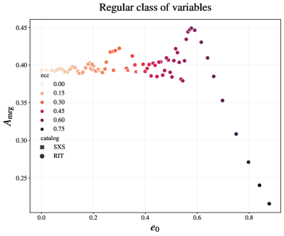
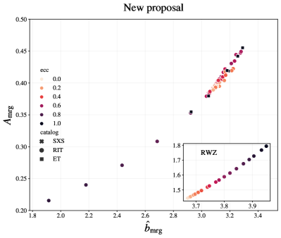
Figure 1: Left panel: merger amplitude as a function of the initial nominal eccentricity attached to the simulations of bounded systems, for equal mass binaries. Their relationship is oscillatory and multi-valued. Right panel: when expressed as a function of a suitably defined dynamical impact parameter evaluated at merger, $\hat{b}_{\rm mrg}=j_{\rm mrg}\,h_{\rm mrg}/\hat{E}_{\mathrm{eff}}^{\mathrm{mrg}}$, where $h\equiv E/M$ ($j\equiv J/m_{1}m_{2}$) is the mass-normalized energy (angular momentum) and $\hat{E}_{\mathrm{eff}}$ is the effective energy of the system per unit mass (in the effective-one-body sense [1]), the same quantity displays a simple monotonic dependence, even for hyperbolic-like systems (square markers). The inset highlights the same relationship for bounded test-mass data.

Noncircular black hole (BH) binary mergers are unique probes of dynamical formation channels in dense environments [2, 3, 4, 5, 6, 7, 8], and allow to push searches of new physics [9, 10] into a stronger-field regime. Gravitational-wave (GW) signals emitted by these systems can be detected by interferometric observatories both on the ground [11, 12] and in space [13], or by Pulsar Timing Arrays [14, 15, 16, 17]. Recently, significant effort has been placed in their modelling and search [18, 19, 20, 21, 22, 23, 24, 25, 26, 27, 28, 29, 30, 31, 32, 33, 34], with one signal already showing evidence of a dynamical capture origin [35]. Crucially, a significant fraction of dynamically-formed sources are expected to lie in the high-end of the mass distribution, due to hierarchical mergers [36, 37, 38, 39, 40, 41, 42], pushing their inspiral outside the sensitive band of ground-based detectors, and giving rise to a signal dominated by the merger-ringdown portion. While several noncircular inspiral models have been developed, both in bounded and dynamically-bounded [43, 44, 45, 46, 47, 48] orbits, merger-ringdown waveforms instead still rely on a quasicircular description [49, 50, 51]. Further, analytical models have shown good accuracy also for scattering orbits [52, 53], a set of configurations which is crucial in the ongoing effort of connecting quantum scattering amplitude calculations with classical gravity [54, 55, 56, 57, 58, 59, 60, 61, 62]. Aside from theoretical considerations, complete noncircular models are urgently needed to extend standard template searches based on quasicircular waveforms [63], which exhibit dramatic sensitivity loss to systems in arbitrary orbits [64]. Laying the foundations to go beyond quasicircular merger-ringdown models is the main goal of this paper.

To this end, appropriate modeling variables capable of capturing the noncircular merger structure are required. For the bounded case, proposed modeling choices in the literature are (non-unique) generalizations of the Newtonian definitions of eccentricity and anomaly parameters. The most recent proposals [65, 66, 67] are based on waveform-constructed quantities, ensuring gauge-invariance. However, these definitions rely on “pericenter” and “apocenter” frequencies constructed from interpolation of the waveform frequency minima and maxima. As a consequence, this method does not apply to situations where only a modest number of waveform cycles is available, which include the vast majority of numerical simulations with intermediate to high eccentricity, and dynamical-capture systems. The above method also requires the specification of an arbitrary reference time at which eccentricity and anomaly are defined; being based on quantities constructed through “orbits”, shortcomings similar to the ones noted above are introduced. Finally, an eccentricity defined from frequency minima and maxima is intrinsically ill-defined at merger, nor can be readily extended to the merger resulting from hyperbolic initial conditions. It is thus intuitive to expect that these parameterisations do not allow for a simple plunge-merger-ringdown modelling.

The above difficulties are showcased by the left panel of Fig. 1, displaying the behavior of the merger GW amplitude $A_{\mathrm{mrg}}$ (defined below) in the equal-mass binary case as a function of the initial orbital eccentricity. The displayed one-dimensional relationship presents a highly complex structure and wide bifurcations: the initial eccentricity parameter does not allow for a smooth merger modeling and, already for intermediate eccentricities, it does not uniquely map the noncircular amplitude value. The same result also holds when using the time-evolved and gauge-invariant eccentricity parameter adopted in Refs. [65, 66, 67] for all the reference times available, with the additional issue that the required interpolation fails for the vast majority of the simulations shown, leaving only a very small dataset to be considered. The latter point also prevents to obtain simple relationships when including a gauge-invariant anomaly parameter [67]: the relationship becomes single-valued, but it presents a highly complicated oscillatory structure difficult to resolve with the very few points for which such parameter can be computed. An equivalent behavior has been observed for the late-time ringdown amplitudes, see Fig.10 of Ref. [68].

We improve on the above parameterizations relying on results obtained in the test mass limit, as studied in Ref. [69]. The merger amplitude of a particle in bounded eccentric orbits is a smooth function of a suitably defined dynamical “impact parameter”, as shown in the inset of the right panel in Fig. 1. With this new parametrization, no bifurcations arise and a simple structure underlying the data emerges. One of the main results of this paper will be to show how the same parametrization can be generalized to the comparable mass case, as previewed in the main right panel of Fig. 1. For comparable masses, we also include dynamically-bounded systems, showcasing how our parameterization is applicable to comparable-mass binaries in generic orbits. Note that this is achieved through a single variable representing the two-dimensional space of initial conditions in the non-circular case (“quasi-universality”): this is a highly non-trivial feature attesting the effectiveness of our modeling strategy. In the remainder of the paper we detail the construction and validation of our modeling variables, and of the displayed relationships, which are similarly built for all the key merger parameters, as shown in Fig. 2. The constructed relationships enable the completion of semi-analytical noncircular models, notably increasing their merger-ringdown faithfulness and allowing to obtain matches at the $99\%$ level even in challenging dynamical capture cases [70]. Such models will significantly extend the discovery horizon of GW searches for compact binary coalescences.

Conventions. We use geometric units $c=G=1$. The GW polarizations $h_{+}$ and $h_{\times}$ are decomposed as

$$h_{+}-{\rm i}h_{\times}=r^{-1}\sum_{\ell=2}^{\infty}\sum_{m=-\ell}^{\ell}h_{\ell m}(t)\,{}_{-2}Y_{\ell m}(\iota,\varphi),$$ (1)

where ${}_{-2}Y_{\ell m}$ are the $s=-2$ spin-weighted spherical harmonics, $r$ is the distance from the observer, and $\iota,\varphi$ are the polar and azimuthal angles that define the orientation of the binary with respect to the observer. Each mode $h_{\ell m}(t)$ is decomposed in amplitude $A_{\ell m}(t)$ and phase $\phi_{\ell m}(t)$, as

$$h_{\ell m}(t)=A_{\ell m}(t)\,{\rm e}^{{\rm i}\phi_{\ell m}(t)}\,,$$ (2)

with an instantaneous GW frequency,

$$\omega_{\ell m}(t)\equiv 2\pi f_{\ell m}(t)=\dot{\phi}_{\ell m}(t)\,.$$ (3)

where the dots indicates derivation with respect to time. The individual ADM masses of the two BHs are denoted as $m_{1,2}$, with $M$ = $m_{1}+m_{2}$, the mass ratio $q\equiv m_{1}/m_{2}\geq 1$, and the symmetric mass ratio $\nu=m_{1}m_{2}/M^{2}$. Since we will be focusing on modelling the dominant $(\ell,m)=(2,\pm 2)$ mode, for simplicity we will drop the mode subscript on the amplitude and frequency throughout the remainder of the paper. The full set of available modes is however used in the fluxes computations.

Construction of variables and templates. To model systems in arbitrary orbits, we start by considering the initial ADM energy and angular momentum $(E^{\rm ADM}_{0},J_{0}^{\rm ADM})$ of the binary, i.e. the initial input of any NR simulation. The values of energy and angular momentum at time $t$, $(E(t),J(t))$, are obtained by subtracting from $(E^{\rm ADM}_{0},J_{0}^{\rm ADM})$ the gravitational wave losses (see the Supplemental Material for details), that is

$$E(t) =E_{0}^{\rm ADM}-\int_{t_{0}}^{t}{\dot{E}(t^{\prime})dt^{\prime}}$$ (4)

$$J(t) =J_{0}^{\rm ADM}-\int_{t_{0}}^{t}{\dot{J}(t^{\prime})dt^{\prime}}\,,$$ (5)

where $t_{0}$ is the starting time of the simulation, and $\dot{E}(t),\dot{J}(t)$ are the radiated fluxes of energy and angular momentum. Note that since we focus our attention only on spin-aligned binaries, $J$ is the angular momentum along the $z$-direction, chosen to be orthogonal to the orbital plane, and there are no losses within the plane [71, 72]. We also define the merger quantities $E_{\mathrm{mrg}}\equiv E(t_{\mathrm{mrg}}),J_{\mathrm{mrg}}\equiv J(t_{\mathrm{mrg}})$, where the merger time $t_{\mathrm{mrg}}$ is defined to be the last peak of the quadrupolar waveform amplitude $A_{22}$, before the beginning of the ringdown phase. For generic initial data, this time does not always coincide with the largest maximum of $A_{22}$, which instead can occur at the periastron passage previous to the plunge-merger.

Even when considering merger-evolved quantities, a key point to obtain accurate fits is to use dimensionless variables factoring out the appropriate mass-scaling. In particular, we use the mass-normalized energy $h_{\mathrm{mrg}}\equiv E_{\mathrm{mrg}}/M$ and angular momentum $j_{\mathrm{mrg}}\equiv J_{\mathrm{mrg}}/(\nu M^{2})$. The effective-one-body (EOB) approach to the two-body general relativistic dynamics [1] is a powerful analytical method that maps the dynamics of a two-body system into the dynamics of an effective body of mass $\mu=m_{1}m_{2}/M$ moving into an effective external potential. The map between the real energy $h$ and the effective energy (per unit mass) $\hat{E}_{\mathrm{eff}}\equiv E_{\rm eff}/\mu$ is given by $h(\hat{E}_{\mathrm{eff}},\nu)=\sqrt{1+2\nu(\hat{E}_{\mathrm{eff}}-1)}$ that once inverted yields $\hat{E}_{\mathrm{eff}}(h,\nu)=1+(h^{2}-1)/(2\nu)$, with $\hat{E}_{\mathrm{eff}}^{\mathrm{mrg}}\equiv\hat{E}_{\mathrm{eff}}(h_{\rm mrg},\nu)$. In general, each binary configuration can be characterized by either $(h,j)$ or, equivalently, $(\hat{E}_{\mathrm{eff}},j)$. For scattering configurations, the EOB approach permits to define an impact parameter of the form $b_{\rm EOB}/M=jh/\sqrt{\hat{E}_{\mathrm{eff}}^{2}-1}$, see Eq. (2.29) in Ref. [59]. In the test-mass limit, i.e. the case of a particle moving on a Schwarzschild BH, we have $h\to 1$, while $\hat{E}_{\mathrm{eff}}$ becomes the real energy of the particle. The parameter $b_{\rm EOB}/M$ is well defined only when $\hat{E}_{\mathrm{eff}}>1$ and thus it cannot be straightforwardly applied, as it is our intention, to characterize the dynamics of bound configurations, where $\hat{E}_{\mathrm{eff}}<1$. Thus, inspired by recent results in the test-mass limit [69], we use as dynamical impact parameter at merger the quantity

$$\hat{b}_{\rm mrg}=\dfrac{b_{\rm mrg}}{M}\equiv\dfrac{j_{\rm mrg}\,h(\hat{E}_{\mathrm{eff}}^{\mathrm{mrg}},\nu)}{\hat{E}_{\mathrm{eff}}^{\mathrm{mrg}}}\ ,$$ (6)

that is the one used in the right panel of Fig. 1. As fitting variables, we will employ functions of $\{\hat{E}_{\mathrm{eff}}^{\mathrm{mrg}},j_{\mathrm{mrg}},\hat{b}_{\mathrm{mrg}},\nu\}$, depending on whether we discuss quasi-universal relations, or consider the full dimensionality of the parameter space. This choice of parameters is key to obtain simple and accurate relationships in arbitrary orbits, shifting the focus from orbit-defined parameters, to quantities which more naturally incorporate radiation-reaction effects.

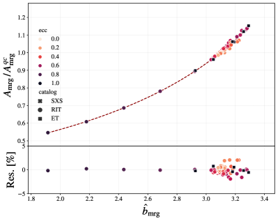
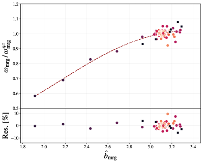
Figure 2: Quasi-universal relationships of the merger quantities in terms of the dimensionless evolved variables. Different marker shapes represent different numerical relativity (NR) simulations catalogs, including both bounded (RIT and SXS) and dynamically bounded (ET) cases, with the data coloured as a function of the nominal eccentricity attached to the simulation. For visual purposes, ET data are assigned a conventional eccentricity value of 1. Note the smaller variation range of $M_{f}$ compared to the other quantities. Smaller panels at the bottom of each figure represent percentage residuals of the fitting template with respect to numerical values. Structures in the residuals indicate small violations of quasi-universality, solved by augmenting the fits with a second variable, making use of the full dimensionality of the parameter space.

The key quantities determining the merger emission are $\{A_{\mathrm{mrg}},\omega_{\mathrm{mrg}},M_{f},a_{f}\}$, where $a_{f}\equiv J_{f}/M_{f}^{2}$, $(M_{f},J_{f})$ denote the mass and spin of the remnant BH, $A_{\rm mrg}\equiv A(t=t_{\mathrm{mrg}})$ and $\omega_{\mathrm{mrg}}\equiv\omega(t=t_{\rm mrg})$. Instead of modeling these quantities directly, we decide to focus on their ratio compared to the quasicircular case. This choice also allows to scale any leading order dependence (e.g. on $\nu$ or $\hat{E}^{\,\mathrm{eff}}_{\mathrm{mrg}}$) which is observed independently of the binary orbital character. It also allows to obtain a factorized form for our fits, which can be straightforwardly be applied on top of quasicircular values [73, 74, 75, 76], maintaining the accuracy of the quasicircular limit where more NR simulations are available. As fitting template, we consider a rational polynomial:

$$Y=Y_{0}\left(\frac{1+p_{1}\,Q+p_{2}\,Q^{2}}{1+p_{3}\,Q+p_{4}\,Q^{2}}\right)\,,$$ (7)

where $Q$ is the dimensionless quantity against which the fit is performed, $Y$ denotes the ratio of the quantities to be modeled with their quasicircular value, and $p_{k}=b_{k}\,(1+c_{k}X)$, with $X\equiv 1-4\nu$, $b_{k},c_{k}\in\mathbb{R}$. Similar to previous work [77], we found this class of functions sufficiently simple and flexible to capture the structure of the merger quantities uncovered by the proposed variables. Residuals are defined by: $\Delta Y\equiv(Y-Y_{\mathrm{NR}})/Y_{\mathrm{NR}}$. Further technical details of the fits are provided in the Supplemental Material. In the latter, we also discuss the procedure which to be followed in practice when incorporating these relationships in an inspiral-plunge-merger-ringdown waveform template.

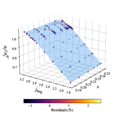
Figure 3: Quasi-universal relationships for the unequal mass dataset (SXS, ET, RIT catalogs, with markers matching the previous figures, and triangles indicating RWZ data), colored according to the obtained residuals. The same structure observed in the equal mass case holds for arbitrary mass ratios, including the test mass limit.

Dataset. We restrict to the nonspinning case and employ 255 publicly available noncircular bounded simulations. The vast majority of them is contained in the fourth public release of the RIT catalog [78], which are complemented by available noncircular simulations from the SXS collaboration [79, 80, 81, 82, 83, 84, 85, 86, 87, 88, 89, 90, 91]. The RIT catalog spans the ranges $q=[1,32]$, $e_{0}=[0,1]$. For the SXS catalog, these intervals restrict to $q=[1,3]$ $e_{0}=[0,0.2]$. Here, $e_{0}$ is the nominal gauge-dependent eccentricity of the simulation evaluated from the binary orbit. Additionally, we employ a custom dataset of dynamical captures simulations generated with the Einstein Toolkit (ET) package [92, 93, 94, 95, 96], with a range $q=[1.0,2.15]$. A detailed description of the latter simulations is available in Ref. [70]. These additional simulations allow us to show that the quasi-universal behavior under investigation is not restricted to initially bound orbits, but is a generic feature of binaries in planar orbits within General Relativity. Finally, we consider also the test-mass data already discussed in Ref. [69]. The latter waveforms are generated by eccentric inspirals of a non-spinning test-particle around a Schwarzschild BH, driven by a suitably resummed EOB-based radiation reaction. They span a large range of eccentricities, and have been computed by numerically solving the Regge-Wheeler and Zerilli (RWZ) inhomogeneous equations [97, 98, 99, 100] with RWZHyp [101, 102, 103].

The computation of the fluxes not only involves the strain modes, but also their time derivatives. Hence, it is important to employ highly accurate waveforms, to avoid outliers stemming from numerical error. We check which simulations are accurate enough for our purposes by verifying that balance laws are satisfied. Integrating throughout the evolution, the following relations need to hold (Eq. (4)):

$$M_{f}=E(t_{\mathrm{end}}),\qquad J_{f}=J(t_{\mathrm{end}})\,,$$ (8)

where $t_{\mathrm{end}}$ is the end time of the simulation. The above relationships might be violated due to numerical error related to finite resolution or to the extrapolation of the waveform to infinity. We find that on the considered dataset, Eq. (8) is typically violated at the $0.1\%$ ($1\%$) level for $M_{f}(J_{f})$. These numbers are fully with the values reported Table II of [104] that refer to the case of quasi-circular binaries. For some simulations, the above relations are violated to a higher degree. Consequently, we apply a “data quality” selection cut, excluding from our dataset all simulations for which Eq. (8) is violated by more than $5\%$. We leave to future work the inclusion of a small amount of simulations displaying a “radial” merger behavior, since their modeling requires accounting for the challenging set of $m=0$ modes, not always well-resolved in current simulations. Details of the latter configurations, together with the full list of simulations used and their properties, are provided in the Supplemental Material.

Results. We start by considering the equal mass case, for which our template has five free parameters. The results of applying Eq. (7) to our dataset are shown in Fig. 2. The merger parameters are well-described by $Q=\hat{b}_{\mathrm{mrg}}$ in Eq. (7), as expected from perturbation theory, while the remnant BH properties $M_{f}/M_{f}^{\rm qc}$ ($a_{f}/a_{f}^{\rm qc}$) are naturally expressed in terms of $Q=\hat{E}^{\,\mathrm{eff}}_{\mathrm{mrg}}$ ($j_{\mathrm{mrg}}$). When considering $A_{\rm mrg}/A_{\mathrm{mrg}}^{\rm qc}$, our model describes the numerical dataset with residuals smaller than $1\%$ for the vast majority of the cases ($87/91$ simulations). This level of discrepancy is fully compatible with the expected numerical error of the simulations [78]. Note the non-monotonic behaviour of the amplitude as a function of eccentricity: a stronger merger emission is observed for moderate eccentricities, while larger eccentricities display a highly suppressed merger amplitude. This non-monotonic behaviour is smoothly accounted for by our dynamical impact parameter, $b_{\mathrm{mrg}}$. In the case of $\omega_{\rm mrg}/\omega_{\rm mrg}^{\rm qc}$, the residuals stay below $3\%$ for the majority of the cases (83/91 simulations), with a few outliers that reach up to $10\%$. We found this quantity to be more strongly affected by the finite numerical resolution (as can be e.g. appreciated comparing the regularity of the patterns in the top left and right panels of Fig. 4). As discussed in Ref. [69], the variation of $\omega_{\mathrm{mrg}}$ with eccentricity is suppressed compared to the amplitude for intermediate eccentricities, hence the impact of numerical noise on this quantity is expected to be larger in the low/mid-eccentricity case. The impact on noncircular corrections on $M_{f}/M_{f}^{\rm qc}$ is the smallest among all considered quantities. It shows the expected monotonic increase as a function of $\hat{E}^{\,\mathrm{eff}}_{\mathrm{mrg}}$, and our parameterization captures its variation with an accuracy better than $0.5\%$ for almost all simulations (89/91 cases). The visual spread of the datapoints with respect to our model is apparently larger compared to the one encountered for other quantities. This variation is, however, fully within the numerical accuracy of this quantity, $O(0.1\%)$, as described in Ref. [78]. Such accuracy is also consistent with our flux-based analysis presented in the previous section. The noncircular behavior of the final Kerr BH angular momentum $a_{f}$ is (again, quite naturally) very well captured by the evolved variable $j_{\mathrm{mrg}}$, with an accuracy better than $1\%$ for almost all the simulations considered (88/91 cases) on the wide range of values present in our dataset (up to $35\%$ variation compared to the quasicircular case).

Error estimation in noncircular binary mergers presents several additional complications compared to the well-studied quasicircular ones. For example, due to the non-monotonicity of the signal frequency, the metric reconstruction cannot be performed by multiplication in the frequency domain with a cutoff [104]. We refer the reader to Ref. [70] for a more in-depth discussion. We leave a detailed study of the impact of numerical error on our modeling strategy to the future, once more accurate or multi-resolution numerical data will become available. However, the smooth structure observed through the proposed method, and the agreement with the behavior observed in the test-mass case [69] (similarly to what happens in the quasicircular case [105, 75]), indicate that a sub-percentage agreement will likely be achieved with higher accuracy data. Finally, it is worth stressing that in Fig. 2 we are quoting residuals relative to the quasicircular case. Since the quantities under consideration have absolute values below unity, for the vast majority of our dataset the error on the absolute values of the noncircular quantities will be smaller than the ones reported.

Although the above dimensional-reduction strategy allows for an accurate representation of the merger quantities in terms of a single effective parameter (quasi-universality), the obtained residuals still show a subdominant trend not fully captured by our parameterization. This has to be expected, since the binary initial conditions in the noncircular case are determined by two of parameters, not a single one. Hence, barring non-trivial simplifications encoded in the binary dynamics, we should not expect a single variable to capture the whole information content. The generalization of the above relationship beyond quasi-universality, including two parameters, is discussed in the Supplemental Material. Although we have mainly focused on studying the simple (quasi-universal) structure uncovered by our variables, such generalizations naturally provide yet smaller residuals than the ones discussed above (given the larger dimensionality of the parameter space employed), allowing to construct even more accurate merger-ringdown waveform models.

Our description maintains a comparable accuracy also in the unequal mass case, where $\nu-$dependent corrections are folded-in through the $p_{k}$ factors in Eq. (7). The number of free parameters are now nine, with no changes in the functional dependence on the fitting variable, compared to the equal mass case. The results are shown in Fig. 3. Even in this extended parameter space, the datapoints lie on a surface, and display smooth changes in terms of $\nu$ and the effective parameters. This is a nontrivial consequence of our effective double-variable parameterisation applied to a system possessing three degrees of freedom. For other common choices of variables, the displayed relationship would not generally be single-valued, and would typically display complex oscillatory structures, akin to Fig. 1. Remarkably, this simple structure holds all the way to the test mass case, which is included in our dataset for the merger quantities. Again, in the Supplemental Material we discuss the extension of these fits beyond quasi-universality. The inclusion of multiple variables has a more pronounced impact on the unequal-mass dataset, bringing the accuracy to the remarkable level already achieved in the equal mass case, with the bulk of the residuals of $O(1\%)$ on $(A_{\rm mrg},a_{f})$, $O(3\%)$ on $\omega_{\rm mrg}$, and $O(0.1\%)$ on $M_{f}$.

Discussion. We have identified the existence of nontrivial order and a simple structure in all public NR simulations of noncircular binaries with nonspinning progenitors. This structure relies on evolved dynamical variables, such as the dynamical impact parameter $\hat{b}_{\mathrm{mrg}}$, uncovering quasi-universal relationships yielding highly accurate models of the merger properties. Such construction, inspired from the behavior observed in the test-mass limit, avoids the issues arising from eccentricity-based parameterizations and frequency peaks interpolations, naturally resolving time ambiguities by evolving up to the merger time. Our results apply equally well to bounded and hyperbolic-like orbits from multiple NR catalogs (including test-mass data), unifying these a priori different regimes into a unique framework. The presented relationships yield the necessary building blocks required to construct highly accurate, semi-analytical full-waveform models, valid for generic planar orbits with mismatches smaller than $1\%$ [70]. They will enable new exciting discoveries of binaries in non-standard configurations, with dramatic implications on our understanding of binary formation in chaotic astrophysical settings.

Our parameterization will also aid the parameter estimation of GW signals sourced by binaries in noncircular orbits. The correlations shown in Fig. 2 of Ref. [35] can now be easily interpreted through our modelling strategy, indicating that the impact parameter is indeed the leading-order measurable quantity characterising such scenarios. The same reasoning applies to the band-like structure observed in the number of encounters as a function of the binary initial conditions [45, 35]. We thus expect our new variables to allow for a much easier sampling convergence (thanks to a much higher degree of smoothness induced by the discussed parameterization), allowing for new observational investigations of GW signals sourced by binaries in generic orbits, previously hindered by computational cost.

Presented results could be extended and improved through an augmented dataset covering a wider range of $\hat{b}_{\rm mrg}$, especially in the hyperbolic case; they would also significantly benefit from higher accuracy simulations. On the other hand, the availability of multiple resolutions for each simulation would enable to incorporate intrinsic errors in our fit. Error inclusion would yield a more robust prediction and allow to discern subdominant features caused by numerical accuracy from the ones that require improved modeling. We expect our strategy to extend without conceptual modifications to spinning binaries, together with the inclusion of higher order modes beyond the leading quadrupolar contribution. These applications will be the subject of future work.

Acknowledgments. We are grateful to Carlos Lousto, James Healy, the Einstein Toolkit community and the SXS collaboration for maintaining the respective public waveform databases and accompanying software. We thank Piero Rettegno, and all the participants to the workshop “EOB@Work 2023” for helpful interactions. G.C. thanks Shilpa Kastha for stimulating interest in this problem and collaboration in the initial attempts to tackle it; David Pereñiguez, Jaime Redondo-Yuste, Maarten van de Meent for fruitful discussions and comments; Luis Lehner and Perimeter Institute for Theoretical Physics for generous hospitality during the last stages of this work. A. N. thanks the Niels Bohr Institute for hospitality during the development of this work. G.C. acknowledges funding from the European Union’s Horizon 2020 research and innovation program under the Marie Sklodowska-Curie grant agreement No. 847523 ‘INTERACTIONS’, from the Villum Investigator program supported by VILLUM FONDEN (grant no. 37766) and the DNRF Chair, by the Danish Research Foundation. R.G. acknowledges support from the Deutsche Forschungsgemeinschaft (DFG) under Grant No. 406116891 within the Research Training Group RTG 2522/1. S.B. knowledges funding from the EU Horizon under ERC Consolidator Grant, no. InspiReM-101043372. The work of T.A. is supported in part by the ERC Advanced Grant GravBHs-692951 and by Grant CEX2019-000918-M funded by Ministerio de Ciencia e Innovación (MCIN)/Agencia Estatal de Investigación (AEI)/10.13039/501100011033. This research was supported in part by Perimeter Institute for Theoretical Physics. Research at Perimeter Institute is supported in part by the Government of Canada through the Department of Innovation, Science and Economic Development Canada and by the Province of Ontario through the Ministry of Colleges and Universities.

Software. We release the dataset behind the figures and a python implementation of our fits in the repository: github.com/GCArullo/noncircular_BBH_fits. This study made use of the open-software python packages: core-watpy, gw_eccentricity, h5py, json, lal, matplotlib, numpy, pandas, pyRing, scipy, seaborn, sxs [106, 67, 107, 108, 109, 110, 111, 112, 113, 114, 115, 116, 117].

Supplemental material

Fluxes computation. The energy and angular momentum fluxes are computed according to:

$$\dot{E} =\frac{1}{16\pi}\,\sum_{\ell=2}^{\ell_{\mathrm{max}}}\sum_{m=-\ell}^{\ell}|\dot{h}_{\ell m}|^{2}$$ (9)

$$\dot{J} =\frac{1}{16\pi}\,\sum_{\ell=2}^{\ell_{\mathrm{max}}}\sum_{m=-\ell}^{\ell}m\cdot\imaginary(h_{\ell m}\cdot\dot{h}^{*}_{\ell m})$$ (10)

with all the available modes: $\ell_{\mathrm{max}}=5$ for RIT, $\ell_{\mathrm{max}}=8$ for SXS, and $\ell_{\mathrm{max}}=8$ for ET data. For ET data we do not include the $m=0$ modes as they are not well-resolved in the simulation. These modes are however completely negligible compared to the total flux for all the configurations considered in this study. Derivatives are computed using centered second order accurate finite-differencing. For data which are equally spaced (such as in the RIT catalog), integrals are computed using second order accurate discrete anti-derivatives, while for unequally spaced data (such as the ones available from the SXS catalog) we use the trapezoidal rule accessed through numpy. We verified that for all the data considered, the time step is sufficiently small that numerical inaccuracies introduce negligible errors. An implementation of the second order accurate formulas we use is publicly available in the core-watpy waveform analysis package [106].

Template implementation. In our study, we construct appropriate variables evaluated at $t_{\rm mrg}$ to model the key merger parameters. Waveform models are instead generated by specifying a set of initial conditions. Hence, when applying our variables to the construction of an inspiral-plunge-merger-ringdown model, the following practical procedure would be followed:

1. Initial conditions are set by ($E_{0}^{\rm ADM},J_{0}^{\rm ADM}$), see Eq. (4), eventually applying the appropriate transformation between EOB and ADM coordinates. An implementation of this step was already achieved in Ref. [35];

2. The pre-merger waveform is used to compute the fluxes entering Eq. (4), yielding ($E(t),J(t)$). A tabulation or analytic representation of the fluxes could also be pre-implemented to reduce the “online” computational cost;

3. The modelling variables $\{\hat{E}_{\mathrm{eff}}^{\mathrm{mrg}},j_{\mathrm{mrg}},\hat{b}_{\mathrm{mrg}}\}$ are constructed using evolved quantities ($E(t),J(t)$), and $\{A_{\mathrm{mrg}},\omega_{\mathrm{mrg}},M_{f},a_{f}\}$ computed through Eq. (7) or Eq. (12);

4. The post-peak model in which $\{A_{\mathrm{mrg}},\omega_{\mathrm{mrg}},M_{f},a_{f}\}$ are used is constructed.

The key point is that quantities discussed in this paper directly enter only the post-merger portion, while fluxes are computed through the pre-merger part of the waveform.

Details of the fits. Lacking a simulation error estimate for our full dataset, we simply use a non-linear least squares algorithm to minimise the difference between our target quantities $\{A_{\mathrm{mrg}},\omega_{\mathrm{mrg}},M_{f},a_{f}\}$ and our template, Eq. (7). We adopt the scipy.optimize.least_squares function, bounding all the coefficients within the interval $[-10,10]$. To avoid missing the minimum of the parameter space the algorithm is exploring, we repeat the fit with 10 different seed values for the coefficients, selecting the seed yielding the coefficients with the smallest value of the cost function. The seed values are extracted from a normal distribution $\mathcal{N}(1,1)$. We verified that the different seeds deliver compatible residuals. This points to a good convergence of the procedure, as expected in a low-dimensional problem when employing a set of variables that allow for a smooth parameterization, such as the ones described in the main text. The resulting coefficients and a python implementation of our factorised fits, which can be straightforwardly applied to augment existing quasicircular ones [73, 74, 75, 76], are publicly available in the repository: github.com/GCArullo/noncircular_BBH_fits.

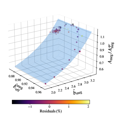
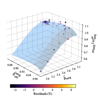
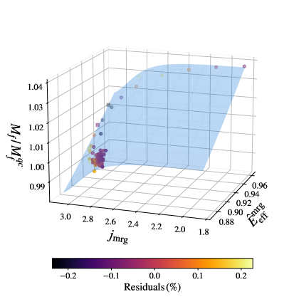
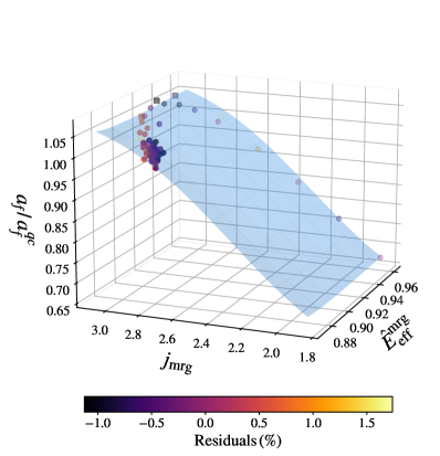
Figure 4: Two-dimensional relationships of the merger quantities in terms of the dimensionless evolved variables for the comparable mass dataset (SXS, ET, RIT, with markers matching the previous figures).

Beyond quasi-universality. In the main text we showed how the merger quantities dependence on the initial conditions can be very well-captured by a single effective parameter. However, at a given initial frequency, the full binary dynamics in the noncircular case is determined by two parameters, typically chosen to be an eccentricity and anomaly parameter in the bounded case. In the scattering case, to go beyond a description based on the impact parameter, one would need to include the asymptotic impulse [118]. To complement $\hat{b}_{\mathrm{mrg}}$, we instead use $\hat{E}_{\mathrm{eff}}^{\mathrm{mrg}}$ as an additional parameter. In the case of the remnant mass, which was already modeled through $\hat{E}_{\mathrm{eff}}^{\mathrm{mrg}}$, we chose instead $j_{\mathrm{mrg}}$.

When using more than one fitting variable, we generalise Eq. (7) to include a product of rational functions, one per fitting quantity:

$$\tilde{Y}=\prod_{i=1}^{2}\,\tilde{Y}_{0}\,\left(\frac{1+p_{1,i}\,Q_{i}+p_{2,i}\,Q_{i}^{2}}{1+p_{3,i}\,Q_{i}+p_{4,i}\,Q_{i}^{2}}\right)\,,$$ (12)

where $p_{k,i}=b_{k,i}\,(1+c_{k,i}X)$ and $b_{k,i},c_{k,i}\in\mathbb{R}$.

The results of these generalized relationships are shown in Fig. 4 for the equal mass case. Although the additional variable helps in resolving subdominant structures present in our dataset, the residuals improvement compared to the single-variable case presented in the main text is modest. This feature is not surprising since the precision of the single-variable relationships was already close to the expected numerical accuracy. Considering that the number of free parameters contained in our new ansatz almost doubled, this shows that $\hat{b}_{\mathrm{mrg}}$ is already capturing close to the whole information content. The residuals of the unequal mass case, depending on three fitting variables, are instead reported as histograms in Fig. 5. In this more general case (except for $a_{f}$), the second fitting variable has a more significant impact: the same remarkable accuracy obtained for the equal-mass case is now maintained also for the full dataset. Improvements to these relationships might come from more accurate NR simulations, or more flexible fitting functions.

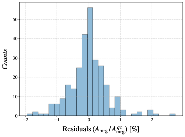
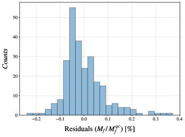
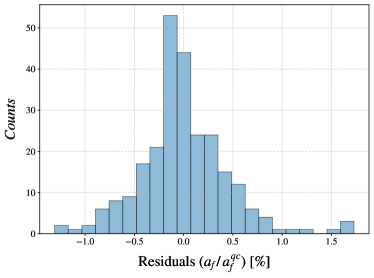
Figure 5: Residuals corresponding to the three variables fits (same combinations as Fig. 4, plus the symmetric mass ratio) for the full dataset.

Simulations dataset. Inspection of the waveform amplitude around merger for highly eccentric simulations reveals that in cases with typical $e_{0}\gtrsim 0.9$, a sharp transition from a smooth morphology to a highly oscillatory one takes place. This change is due to the $(\ell,m)=(2,\pm 2)$ mode becoming almost purely real, a feature which is also observed in the merger-ringdown of test particles undergoing a radial plunge [119, 120]. To obtain a smooth quantity amenable to modelling, in these cases it is necessary to consider the combined amplitude of all the modes beyond the dominant one, including $m=0$ modes. The transition to this “radial” behaviour happens sharply for $A_{\mathrm{mrg}}/\nu\simeq 0.8$. In these cases, multiple $A_{22}$ local maxima are observed during the ringdown phase, and a $t_{\mathrm{mrg}}$ definition taking into account higher modes is required. Since the purpose of this study is to model the dominant mode, $(\ell,m)=(2,\pm 2)$, we do not include such simulations in our dataset. For the same reason, we do not include simulations with $q>3$.

The considered simulations and their relevant parameters are given in the tables below. Tab. LABEL:tab:sims reports the list of full numerical simulations, and Tab. 2 reports test-mass data.

Table 1: List of full numerical simulations included in our dataset, and selected associated parameters.

Catalog	ID	q	$e_{0}$	$E^{ADM}_{0}$	$J^{ADM}_{0}$	$\hat{E}_{\mathrm{eff}}^{\mathrm{mrg}}$	$j_{\mathrm{mrg}}$	$\hat{b}_{\mathrm{mrg}}$
RIT	1090	1.0000	0.0000	0.9907	1.0028	0.8812	2.8108	3.0935
RIT	1091	1.0000	0.0020	0.9907	1.0018	0.8808	2.8083	3.0920
RIT	1092	1.0000	0.0040	0.9907	1.0008	0.8808	2.8079	3.0915
RIT	1093	1.0000	0.0060	0.9907	0.9998	0.8809	2.8088	3.0922
RIT	1094	1.0000	0.0080	0.9906	0.9988	0.8817	2.8141	3.0958
RIT	1095	1.0000	0.0100	0.9906	0.9978	0.8810	2.8099	3.0930
RIT	1096	1.0000	0.0150	0.9906	0.9953	0.8810	2.8106	3.0939
RIT	1097	1.0000	0.0200	0.9905	0.9927	0.8807	2.8095	3.0935
RIT	1098	1.0000	0.0400	0.9903	0.9825	0.8839	2.8241	3.1010
RIT	1099	1.0000	0.0500	0.9901	0.9774	0.8805	2.8050	3.0891
RIT	1100	1.0000	0.0600	0.9900	0.9723	0.8801	2.8084	3.0940
RIT	1101	1.0000	0.0700	0.9899	0.9671	0.8821	2.8226	3.1039
RIT	1102	1.0000	0.0800	0.9898	0.9619	0.8830	2.8219	3.1008
RIT	1103	1.0000	0.0900	0.9897	0.9566	0.8817	2.8078	3.0888
RIT	1104	1.0000	0.1000	0.9896	0.9513	0.8808	2.8070	3.0905
RIT	1105	1.0000	0.1100	0.9894	0.9460	0.8822	2.8266	3.1081
RIT	1106	1.0000	0.1200	0.9893	0.9407	0.8831	2.8348	3.1149
RIT	1107	1.0000	0.1300	0.9892	0.9354	0.8833	2.8278	3.1067
RIT	1108	1.0000	0.1400	0.9891	0.9300	0.8830	2.8134	3.0915
RIT	1109	1.0000	0.1450	0.9890	0.9273	0.8818	2.8023	3.0826
RIT	1110	1.0000	0.1570	0.9889	0.9207	0.8784	2.7928	3.0811
RIT	1111	1.0000	0.1600	0.9889	0.9191	0.8784	2.7985	3.0874
RIT	1112	1.0000	0.1700	0.9887	0.9136	0.8790	2.8185	3.1080
RIT	1113	1.0000	0.1800	0.9886	0.9081	0.8833	2.8486	3.1295
RIT	1114	1.0000	0.1850	0.9886	0.9053	0.8849	2.8556	3.1329
RIT	1115	1.0000	0.1950	0.9884	0.8997	0.8863	2.8527	3.1257
RIT	1116	1.0000	0.2000	0.9884	0.8969	0.8877	2.8519	3.1212
RIT	1117	1.0000	0.2100	0.9883	0.8913	0.8876	2.8320	3.0998
RIT	1118	1.0000	0.2350	0.9880	0.8771	0.8752	2.7837	3.0799
RIT	1119	1.0000	0.2450	0.9879	0.8713	0.8792	2.8352	3.1258
RIT	1120	1.0000	0.2500	0.9878	0.8685	0.8857	2.8834	3.1612
RIT	1121	1.0000	0.2650	0.9876	0.8597	0.8832	2.8837	3.1682
RIT	1122	1.0000	0.2750	0.9875	0.8539	0.8868	2.9052	3.1819
RIT	1123	1.0000	0.2850	0.9874	0.8479	0.8977	2.9618	3.2138
RIT	1124	1.0000	0.3000	0.9872	0.8390	0.9049	2.9894	3.2242
RIT	1125	1.0000	0.3500	0.9866	0.8085	0.9114	2.9560	3.1707
RIT	1201	2.0000	0.0020	0.9918	0.8910	0.8904	2.8875	3.1629
RIT	1202	2.0000	0.0040	0.9917	0.8901	0.8882	2.8743	3.1545
RIT	1203	2.0000	0.0060	0.9917	0.8892	0.8885	2.8760	3.1558
RIT	1204	2.0000	0.0080	0.9917	0.8883	0.8884	2.8752	3.1552
RIT	1205	2.0000	0.0100	0.9917	0.8874	0.8885	2.8758	3.1554
RIT	1206	2.0000	0.0150	0.9916	0.8851	0.8888	2.8770	3.1560
RIT	1207	2.0000	0.0200	0.9916	0.8829	0.8884	2.8746	3.1544
RIT	1208	2.0000	0.0300	0.9915	0.8784	0.8903	2.8890	3.1648
RIT	1209	2.0000	0.0400	0.9914	0.8738	0.8892	2.8830	3.1614
RIT	1210	2.0000	0.0500	0.9913	0.8693	0.8910	2.8889	3.1629
RIT	1211	2.0000	0.0600	0.9912	0.8647	0.8879	2.8697	3.1505
RIT	1212	2.0000	0.0700	0.9910	0.8601	0.8877	2.8763	3.1582
RIT	1213	2.0000	0.0800	0.9909	0.8554	0.8890	2.8863	3.1656
RIT	1214	2.0000	0.0900	0.9908	0.8508	0.8926	2.8998	3.1703
RIT	1215	2.0000	0.1000	0.9907	0.8461	0.8894	2.8741	3.1511
RIT	1216	2.0000	0.1100	0.9906	0.8414	0.8860	2.8635	3.1489
RIT	1217	2.0000	0.1200	0.9905	0.8366	0.8910	2.9046	3.1800
RIT	1218	2.0000	0.1300	0.9904	0.8319	0.8913	2.9046	3.1790
RIT	1219	2.0000	0.1400	0.9903	0.8271	0.8933	2.9031	3.1718
RIT	1220	2.0000	0.1500	0.9902	0.8222	0.8912	2.8793	3.1518
RIT	1221	2.0000	0.1600	0.9901	0.8174	0.8865	2.8626	3.1467
RIT	1222	2.0000	0.1700	0.9900	0.8125	0.8877	2.8904	3.1738
RIT	1223	2.0000	0.1800	0.9899	0.8076	0.8897	2.9101	3.1898
RIT	1224	2.0000	0.1900	0.9898	0.8027	0.8963	2.9433	3.2071
RIT	1226	2.0000	0.2100	0.9896	0.7927	0.8926	2.8832	3.1522
RIT	1227	2.0000	0.2200	0.9895	0.7877	0.8903	2.8652	3.1388
RIT	1228	2.0000	0.2300	0.9894	0.7826	0.8848	2.8608	3.1494
RIT	1229	2.0000	0.2400	0.9893	0.7775	0.8848	2.8919	3.1837
RIT	1230	2.0000	0.2500	0.9892	0.7724	0.8931	2.9587	3.2331
RIT	1231	2.0000	0.2700	0.9890	0.7620	0.8993	2.9990	3.2594
RIT	1232	2.0000	0.3000	0.9886	0.7462	0.9132	3.0524	3.2775
RIT	1241	1.3333	0.0000	0.9909	0.9824	0.8824	2.8210	3.1034
RIT	1242	1.3333	0.0020	0.9909	0.9814	0.8827	2.8224	3.1043
RIT	1243	1.3333	0.0040	0.9909	0.9805	0.8824	2.8204	3.1029
RIT	1244	1.3333	0.0060	0.9909	0.9795	0.8824	2.8205	3.1030
RIT	1245	1.3333	0.0080	0.9908	0.9785	0.8819	2.8178	3.1013
RIT	1246	1.3333	0.0100	0.9908	0.9775	0.8829	2.8233	3.1048
RIT	1247	1.3333	0.0150	0.9908	0.9750	0.8825	2.8222	3.1045
RIT	1248	1.3333	0.0200	0.9907	0.9726	0.8830	2.8255	3.1070
RIT	1249	1.3333	0.0300	0.9906	0.9676	0.8819	2.8201	3.1039
RIT	1250	1.3333	0.0400	0.9905	0.9626	0.8831	2.8237	3.1046
RIT	1251	1.3333	0.0500	0.9904	0.9576	0.8822	2.8177	3.1005
RIT	1252	1.3333	0.0600	0.9902	0.9525	0.8827	2.8265	3.1086
RIT	1253	1.3333	0.0700	0.9901	0.9474	0.8822	2.8271	3.1107
RIT	1254	1.3333	0.0800	0.9900	0.9423	0.8835	2.8296	3.1100
RIT	1255	1.3333	0.0900	0.9899	0.9372	0.8828	2.8177	3.0989
RIT	1256	1.3333	0.1000	0.9898	0.9320	0.8835	2.8249	3.1048
RIT	1257	1.3333	0.1100	0.9897	0.9268	0.8834	2.8361	3.1173
RIT	1258	1.3333	0.1200	0.9895	0.9216	0.8835	2.8411	3.1228
RIT	1259	1.3333	0.1300	0.9894	0.9164	0.8875	2.8576	3.1298
RIT	1260	1.3333	0.1400	0.9893	0.9111	0.8847	2.8275	3.1045
RIT	1261	1.3333	0.1500	0.9892	0.9058	0.8849	2.8244	3.1004
RIT	1262	1.3333	0.1600	0.9891	0.9004	0.8799	2.8099	3.0981
RIT	1263	1.3333	0.1700	0.9890	0.8950	0.8810	2.8340	3.1216
RIT	1264	1.3333	0.1800	0.9889	0.8896	0.8847	2.8608	3.1411
RIT	1265	1.3333	0.1900	0.9887	0.8842	0.8886	2.8769	3.1480
RIT	1266	1.3333	0.2000	0.9886	0.8787	0.8892	2.8648	3.1331
RIT	1267	1.3333	0.2100	0.9885	0.8732	0.8880	2.8387	3.1077
RIT	1268	1.3333	0.2200	0.9884	0.8677	0.8832	2.8025	3.0810
RIT	1269	1.3333	0.2300	0.9883	0.8621	0.8805	2.8054	3.0917
RIT	1270	1.3333	0.2400	0.9882	0.8565	0.8779	2.8219	3.1167
RIT	1271	1.3333	0.2500	0.9880	0.8508	0.8867	2.8954	3.1734
RIT	1272	1.3333	0.2700	0.9878	0.8394	0.8872	2.9120	3.1902
RIT	1273	1.3333	0.3000	0.9875	0.8220	0.9042	2.9885	3.2265
RIT	1274	1.3333	0.3500	0.9869	0.7921	0.9132	2.9680	3.1802
RIT	1282	1.0000	0.1900	0.9943	1.2099	0.8810	2.8193	3.1035
RIT	1283	1.0000	0.2775	0.9938	1.1427	0.8825	2.8190	3.0991
RIT	1284	1.0000	0.3276	0.9936	1.1024	0.8797	2.8076	3.0941
RIT	1285	1.0000	0.3600	0.9934	1.0755	0.8827	2.8292	3.1097
RIT	1286	1.0000	0.3994	0.9932	1.0419	0.8841	2.8052	3.0797
RIT	1287	1.0000	0.3916	0.9932	1.0486	0.8826	2.8339	3.1152
RIT	1288	1.0000	0.4148	0.9931	1.0284	0.8849	2.8346	3.1096
RIT	1289	1.0000	0.4071	0.9932	1.0351	0.8782	2.8022	3.0922
RIT	1290	1.0000	0.4300	0.9930	1.0150	0.8810	2.8310	3.1162
RIT	1291	1.0000	0.4224	0.9931	1.0217	0.8790	2.7721	3.0569
RIT	1292	1.0000	0.4450	0.9930	1.0015	0.8769	2.7606	3.0496
RIT	1293	1.0000	0.4375	0.9930	1.0083	0.8872	2.8383	3.1075
RIT	1294	1.0000	0.4598	0.9929	0.9881	0.8903	2.8707	3.1348
RIT	1295	1.0000	0.4524	0.9929	0.9948	0.8806	2.8327	3.1192
RIT	1296	1.0000	0.4744	0.9928	0.9746	0.8745	2.7812	3.0788
RIT	1297	1.0000	0.4671	0.9928	0.9814	0.8834	2.7850	3.0593
RIT	1298	1.0000	0.4888	0.9927	0.9612	0.8895	2.8682	3.1341
RIT	1299	1.0000	0.4816	0.9928	0.9679	0.8863	2.8747	3.1501
RIT	1300	1.0000	0.5030	0.9927	0.9478	0.8752	2.7620	3.0559
RIT	1301	1.0000	0.4959	0.9927	0.9545	0.8893	2.8178	3.0797
RIT	1302	1.0000	0.5170	0.9926	0.9343	0.8868	2.8909	3.1662
RIT	1303	1.0000	0.5100	0.9926	0.9410	0.8800	2.8455	3.1350
RIT	1304	1.0000	0.5308	0.9925	0.9209	0.8908	2.8536	3.1148
RIT	1305	1.0000	0.5239	0.9925	0.9276	0.8898	2.8872	3.1541
RIT	1306	1.0000	0.5444	0.9924	0.9074	0.8700	2.7304	3.0345
RIT	1307	1.0000	0.5376	0.9925	0.9142	0.8865	2.7831	3.0490
RIT	1308	1.0000	0.5578	0.9924	0.8940	0.8952	2.9740	3.2341
RIT	1309	1.0000	0.5511	0.9924	0.9007	0.8732	2.8194	3.1246
RIT	1310	1.0000	0.5710	0.9923	0.8805	0.9090	3.0481	3.2762
RIT	1311	1.0000	0.5644	0.9923	0.8873	0.8972	2.9883	3.2441
RIT	1312	1.0000	0.5775	0.9923	0.8738	0.9145	3.0661	3.2802
RIT	1313	1.0000	0.5904	0.9922	0.8604	0.9238	3.0839	3.2740
RIT	1314	1.0000	0.6156	0.9921	0.8335	0.9313	3.0430	3.2108
RIT	1315	1.0000	0.6400	0.9919	0.8066	0.9384	2.9915	3.1383
RIT	1316	1.0000	0.6636	0.9918	0.7797	0.9431	2.9224	3.0542
RIT	1317	1.0000	0.6975	0.9916	0.7394	0.9493	2.8101	2.9223
RIT	1318	1.0000	0.7500	0.9914	0.6722	0.9555	2.5943	2.6848
RIT	1319	1.0000	0.7975	0.9911	0.6050	0.9589	2.3597	2.4355
RIT	1320	1.0000	0.8400	0.9909	0.5377	0.9608	2.1145	2.1792
RIT	1321	1.0000	0.8775	0.9907	0.4705	0.9613	1.8592	1.9152
RIT	1330	1.1111	0.1900	0.9943	1.2077	0.8813	2.8053	3.0874
RIT	1331	1.1111	0.3600	0.9934	1.0735	0.8812	2.8199	3.1039
RIT	1332	1.1111	0.4375	0.9930	1.0064	0.8870	2.8459	3.1168
RIT	1333	1.1111	0.4671	0.9929	0.9796	0.8869	2.8097	3.0773
RIT	1334	1.1111	0.5100	0.9926	0.9393	0.8754	2.8155	3.1148
RIT	1335	1.1111	0.5511	0.9924	0.8990	0.8707	2.8002	3.1107
RIT	1336	1.1111	0.5775	0.9923	0.8722	0.9148	3.0699	3.2837
RIT	1337	1.1111	0.6156	0.9921	0.8319	0.9322	3.0506	3.2167
RIT	1338	1.1111	0.6400	0.9920	0.8051	0.9402	3.0044	3.1474
RIT	1339	1.1111	0.6636	0.9918	0.7783	0.9436	2.9278	3.0588
RIT	1340	1.1111	0.6975	0.9917	0.7380	0.9497	2.8145	2.9262
RIT	1341	1.1111	0.7500	0.9914	0.6709	0.9556	2.5977	2.6880
RIT	1342	1.1111	0.7975	0.9911	0.6038	0.9589	2.3623	2.4382
RIT	1343	1.1111	0.8400	0.9909	0.5367	0.9608	2.1167	2.1814
RIT	1344	1.1111	0.8775	0.9907	0.4696	0.9613	1.8610	1.9171
RIT	1353	1.2500	0.1900	0.9944	1.1961	0.8830	2.8237	3.1040
RIT	1354	1.2500	0.3600	0.9935	1.0632	0.8801	2.8136	3.1008
SXS	1355	1.0000	0.0678	0.9921	1.0719	0.8783	2.8044	3.0945
SXS	1356	1.0000	0.1975	0.9934	1.1467	0.8811	2.8096	3.0925
SXS	1357	1.0000	0.2211	0.9924	1.0823	0.8821	2.8049	3.0846
SXS	1358	1.0000	0.2186	0.9923	1.0759	0.8811	2.8094	3.0924
SXS	1359	1.0000	0.2178	0.9923	1.0721	0.8824	2.8156	3.0955
SXS	1360	1.0000	0.3636	0.9924	1.0682	0.8788	2.7941	3.0818
SXS	1361	1.0000	0.3326	0.9923	1.0668	0.8802	2.8009	3.0855
SXS	1362	1.0000	0.0000	0.9925	1.0619	0.8828	2.8098	3.0881
SXS	1363	1.0000	0.0000	0.9925	1.0608	0.8823	2.7970	3.0754
RIT	1364	1.2500	0.7500	0.9915	0.6645	0.9557	2.5986	2.6890
RIT	1365	1.2500	0.7975	0.9912	0.5980	0.9590	2.3629	2.4389
RIT	1366	1.2500	0.8400	0.9910	0.5316	0.9608	2.1171	2.1820
RIT	1367	1.2500	0.8775	0.9908	0.4651	0.9614	1.8612	1.9174
RIT	1376	1.4286	0.1900	0.9945	1.1733	0.8831	2.8291	3.1117
RIT	1377	1.4286	0.3600	0.9936	1.0429	0.8783	2.7979	3.0901
RIT	1378	1.4286	0.4375	0.9932	0.9778	0.8884	2.8689	3.1409
RIT	1379	1.4286	0.4671	0.9931	0.9517	0.8876	2.8258	3.0957
RIT	1380	1.4286	0.5100	0.9929	0.9126	0.8802	2.8507	3.1433
RIT	1381	1.4286	0.5511	0.9926	0.8735	0.8856	2.9036	3.1865
RIT	1382	1.4286	0.5775	0.9925	0.8474	0.9222	3.1162	3.3147
RIT	1383	1.4286	0.6156	0.9923	0.8083	0.9333	3.0588	3.2241
RIT	1384	1.4286	0.6400	0.9922	0.7822	0.9377	2.9921	3.1424
RIT	1385	1.4286	0.6636	0.9921	0.7561	0.9444	2.9337	3.0643
RIT	1386	1.4286	0.6975	0.9919	0.7170	0.9502	2.8189	2.9306
RIT	1387	1.4286	0.7500	0.9916	0.6518	0.9559	2.6004	2.6911
RIT	1388	1.4286	0.7975	0.9914	0.5867	0.9591	2.3640	2.4403
RIT	1389	1.4286	0.8400	0.9912	0.5215	0.9609	2.1177	2.1830
RIT	1390	1.4286	0.8775	0.9910	0.4563	0.9614	1.8616	1.9182
RIT	1399	1.6667	0.1900	0.9947	1.1353	0.8858	2.8528	3.1333
RIT	1400	1.6667	0.3600	0.9938	1.0092	0.8841	2.8180	3.0996
RIT	1401	1.6667	0.4375	0.9934	0.9461	0.8887	2.8852	3.1606
RIT	1402	1.6667	0.4671	0.9933	0.9209	0.8908	2.8579	3.1252
RIT	1403	1.6667	0.5100	0.9931	0.8830	0.8840	2.8811	3.1693
RIT	1404	1.6667	0.5511	0.9929	0.8452	0.9007	3.0131	3.2665
RIT	1405	1.6667	0.5775	0.9928	0.8200	0.9244	3.1327	3.3283
RIT	1406	1.6667	0.6156	0.9926	0.7821	0.9345	3.0680	3.2324
RIT	1407	1.6667	0.6400	0.9924	0.7569	0.9442	3.0304	3.1673
RIT	1408	1.6667	0.6636	0.9923	0.7316	0.9462	2.9457	3.0736
RIT	1409	1.6667	0.6975	0.9922	0.6938	0.9536	2.8405	2.9461
RIT	1410	1.6667	0.7500	0.9919	0.6307	0.9563	2.6036	2.6945
RIT	1411	1.6667	0.7975	0.9917	0.5677	0.9593	2.3661	2.4428
RIT	1412	1.6667	0.8400	0.9915	0.5046	0.9610	2.1189	2.1847
RIT	1413	1.6667	0.8775	0.9913	0.4415	0.9615	1.8633	1.9203
RIT	1422	2.0000	0.1900	0.9949	1.0755	0.8889	2.8819	3.1612
RIT	1423	2.0000	0.3600	0.9941	0.9560	0.8912	2.8819	3.1546
RIT	1424	2.0000	0.4375	0.9938	0.8963	0.8907	2.9129	3.1899
RIT	1425	2.0000	0.4671	0.9936	0.8724	0.8934	2.8901	3.1574
RIT	1426	2.0000	0.5100	0.9934	0.8365	0.8899	2.9329	3.2140
RIT	1427	2.0000	0.5511	0.9932	0.8007	0.9038	3.0511	3.3029
RIT	1428	2.0000	0.5775	0.9931	0.7768	0.9259	3.1454	3.3408
RIT	1429	2.0000	0.6156	0.9929	0.7409	0.9401	3.1012	3.2545
RIT	1430	2.0000	0.6400	0.9928	0.7170	0.9460	3.0417	3.1765
RIT	1431	2.0000	0.6636	0.9927	0.6931	0.9480	2.9563	3.0821
RIT	1432	2.0000	0.6975	0.9926	0.6573	0.9530	2.8362	2.9449
RIT	1433	2.0000	0.7500	0.9923	0.5975	0.9572	2.6086	2.6992
RIT	1434	2.0000	0.7975	0.9921	0.5378	0.9598	2.3689	2.4458
RIT	1435	2.0000	0.8400	0.9919	0.4780	0.9612	2.1201	2.1865
RIT	1436	2.0000	0.8775	0.9917	0.4183	0.9616	1.8627	1.9205
RIT	1445	2.5000	0.1900	0.9953	0.9886	0.8931	2.9277	3.2058
RIT	1446	2.5000	0.3600	0.9946	0.8787	0.8905	2.8916	3.1737
RIT	1447	2.5000	0.4375	0.9943	0.8238	0.8892	2.9052	3.1925
RIT	1448	2.5000	0.4671	0.9942	0.8018	0.9026	2.9890	3.2451
RIT	1449	2.5000	0.5100	0.9940	0.7689	0.8937	2.9715	3.2521
RIT	1450	2.5000	0.5511	0.9938	0.7359	0.9117	3.1204	3.3603
RIT	1451	2.5000	0.5775	0.9937	0.7140	0.9328	3.1961	3.3791
RIT	1452	2.5000	0.6156	0.9935	0.6810	0.9421	3.1204	3.2729
RIT	1453	2.5000	0.6400	0.9934	0.6590	0.9483	3.0620	3.1946
RIT	1454	2.5000	0.6636	0.9933	0.6371	0.9508	2.9788	3.1012
RIT	1455	2.5000	0.6975	0.9932	0.6041	0.9550	2.8535	2.9605
RIT	1456	2.5000	0.7500	0.9929	0.5492	0.9584	2.6206	2.7110
RIT	1457	2.5000	0.7975	0.9927	0.4943	0.9605	2.3770	2.4547
RIT	1458	2.5000	0.8400	0.9926	0.4394	0.9614	2.1244	2.1922
RIT	1459	2.5000	0.8775	0.9924	0.3844	0.9617	1.8658	1.9249
RIT	1468	3.0000	0.1900	0.9957	0.9075	0.8967	2.9637	3.2406
RIT	1469	3.0000	0.3600	0.9951	0.8067	0.8985	2.9763	3.2489
RIT	1470	3.0000	0.4375	0.9947	0.7563	0.8934	2.9121	3.1937
RIT	1471	3.0000	0.4671	0.9946	0.7361	0.9045	3.0281	3.2872
RIT	1472	3.0000	0.5100	0.9945	0.7059	0.9033	3.0514	3.3161
RIT	1473	3.0000	0.5511	0.9943	0.6756	0.9155	3.1599	3.3964
RIT	1474	3.0000	0.5775	0.9942	0.6555	0.9372	3.2278	3.4033
RIT	1475	3.0000	0.6156	0.9940	0.6252	0.9464	3.1486	3.2932
RIT	1476	3.0000	0.6400	0.9940	0.6050	0.9505	3.0767	3.2067
RIT	1477	3.0000	0.6636	0.9939	0.5849	0.9528	2.9916	3.1119
RIT	1478	3.0000	0.6975	0.9937	0.5546	0.9564	2.8630	2.9689
RIT	1479	3.0000	0.7500	0.9935	0.5042	0.9593	2.6266	2.7169
RIT	1480	3.0000	0.7975	0.9933	0.4538	0.9610	2.3803	2.4587
RIT	1481	3.0000	0.8400	0.9932	0.4034	0.9617	2.1261	2.1948
RIT	1482	3.0000	0.8775	0.9930	0.3529	0.9618	1.8665	1.9267
ET	37	1.0000	1.0000	0.9943	0.7432	0.9621	2.8421	2.9259
ET	42	1.0000	1.0000	0.9943	0.8263	0.9456	3.0592	3.1909
ET	42_q150	1.5000	1.0000	0.9950	0.8263	0.9382	3.1313	3.2875
ET	42_q200	2.0000	1.0000	0.9964	0.8263	0.9056	3.0975	3.3479
ET	42_q215	2.1500	1.0000	0.9969	0.8263	0.9140	3.0779	3.3041
ET	44	1.0000	1.0000	0.9943	0.8579	0.9301	3.0833	3.2566
ET	46	1.0000	1.0000	0.9943	0.8883	0.9123	3.0702	3.2907
ET	48	1.0000	1.0000	0.9943	0.9177	0.8728	2.7504	3.0493
ET	50	1.0000	1.0000	0.9943	0.9460	0.8874	2.9056	3.1806

Table 2: List of test-mass data included in our dataset, and selected associated parameters. All evolutions start at apastron.

Catalog	ID	$e_{0}$	$\hat{E}_{\mathrm{eff}}^{\mathrm{mrg}}$	$j_{\mathrm{mrg}}$	$\hat{b}_{\mathrm{mrg}}$
RWZ	1	0.0000	0.9423	3.4577	3.6695
RWZ	2	0.0500	0.9425	3.4602	3.6714
RWZ	3	0.1000	0.9430	3.4671	3.6768
RWZ	4	0.1500	0.9433	3.4720	3.6805
RWZ	5	0.2000	0.9444	3.4859	3.6911
RWZ	6	0.2500	0.9451	3.4936	3.6967
RWZ	7	0.3000	0.9463	3.5085	3.7077
RWZ	8	0.3500	0.9477	3.5247	3.7193
RWZ	9	0.4000	0.9504	3.5548	3.7403
RWZ	10	0.4500	0.9513	3.5649	3.7473
RWZ	11	0.5000	0.9546	3.5989	3.7702
RWZ	12	0.5500	0.9563	3.6165	3.7817
RWZ	13	0.6000	0.9593	3.6453	3.8001
RWZ	14	0.6500	0.9626	3.6774	3.8203
RWZ	15	0.7000	0.9666	3.7149	3.8433
RWZ	16	0.7500	0.9711	3.7562	3.8681
RWZ	17	0.8000	0.9752	3.7921	3.8885
RWZ	18	0.8500	0.9785	3.8212	3.9050
RWZ	19	0.9000	0.9841	3.8696	3.9321
RWZ	20	0.9500	0.9880	3.9017	3.9492

References

- Buonanno and Damour [1999] A. Buonanno and T. Damour, Phys. Rev. D59, 084006 (1999), arXiv:gr-qc/9811091 .
- Samsing [2018] J. Samsing, Phys. Rev. D97, 103014 (2018), arXiv:1711.07452 [astro-ph.HE] .
- Zevin et al. [2019] M. Zevin, J. Samsing, C. Rodriguez, C.-J. Haster, and E. Ramirez-Ruiz, Astrophys. J. 871, 91 (2019), arXiv:1810.00901 [astro-ph.HE] .
- Tagawa et al. [2021a] H. Tagawa, B. Kocsis, Z. Haiman, I. Bartos, K. Omukai, and J. Samsing, Astrophys. J. Lett. 907, L20 (2021a), arXiv:2010.10526 [astro-ph.HE] .
- Samsing et al. [2022] J. Samsing, I. Bartos, D. J. D’Orazio, Z. Haiman, B. Kocsis, N. W. C. Leigh, B. Liu, M. E. Pessah, and H. Tagawa, Nature 603, 237 (2022), arXiv:2010.09765 [astro-ph.HE] .
- Zevin et al. [2021] M. Zevin, I. M. Romero-Shaw, K. Kremer, E. Thrane, and P. D. Lasky, Astrophys. J. Lett. 921, L43 (2021), arXiv:2106.09042 [astro-ph.HE] .
- Fragione et al. [2021] G. Fragione, B. Kocsis, F. A. Rasio, and J. Silk, arXiv e-prints , arXiv:2107.04639 (2021), arXiv:2107.04639 [astro-ph.GA] .
- Chattopadhyay et al. [2023] D. Chattopadhyay, J. Stegmann, F. Antonini, J. Barber, and I. M. Romero-Shaw, (2023), arXiv:2308.10884 [astro-ph.HE] .
- Abbott et al. [2021a] R. Abbott et al. (LIGO Scientific, VIRGO, KAGRA), (2021a), arXiv:2112.06861 [gr-qc] .
- Narayan et al. [2023] P. Narayan, N. K. Johnson-McDaniel, and A. Gupta, (2023), arXiv:2306.04068 [gr-qc] .
- Aasi et al. [2015] J. Aasi et al. (LIGO Scientific), Class. Quant. Grav. 32, 074001 (2015), arXiv:1411.4547 [gr-qc] .
- Acernese et al. [2015] F. Acernese et al. (VIRGO), Class. Quant. Grav. 32, 024001 (2015), arXiv:1408.3978 [gr-qc] .
- Amaro-Seoane et al. [2017] P. Amaro-Seoane et al. (LISA), (2017), arXiv:1702.00786 [astro-ph.IM] .
- Antoniadis et al. [2023] J. Antoniadis et al., (2023), arXiv:2306.16214 [astro-ph.HE] .
- Agazie et al. [2023] G. Agazie et al. (NANOGrav), Astrophys. J. Lett. 951, L8 (2023), arXiv:2306.16213 [astro-ph.HE] .
- Reardon et al. [2023] D. J. Reardon et al., Astrophys. J. Lett. 951, L6 (2023), arXiv:2306.16215 [astro-ph.HE] .
- Xu et al. [2023] H. Xu et al., Res. Astron. Astrophys. 23, 075024 (2023), arXiv:2306.16216 [astro-ph.HE] .
- Abbott et al. [2019] B. P. Abbott et al. (LIGO Scientific, Virgo), Astrophys. J. 883, 149 (2019), arXiv:1907.09384 [astro-ph.HE] .
- Romero-Shaw et al. [2019] I. M. Romero-Shaw, P. D. Lasky, and E. Thrane, Mon. Not. Roy. Astron. Soc. 490, 5210 (2019), arXiv:1909.05466 [astro-ph.HE] .
- Nitz et al. [2019] A. H. Nitz, A. Lenon, and D. A. Brown, Astrophys. J. 890, 1 (2019), arXiv:1912.05464 [astro-ph.HE] .
- Gayathri et al. [2022] V. Gayathri, J. Healy, J. Lange, B. O’Brien, M. Szczepanczyk, I. Bartos, M. Campanelli, S. Klimenko, C. O. Lousto, and R. O’Shaughnessy, Nature Astron. 6, 344 (2022), arXiv:2009.05461 [astro-ph.HE] .
- Ramos-Buades et al. [2020] A. Ramos-Buades, S. Tiwari, M. Haney, and S. Husa, Phys. Rev. D 102, 043005 (2020), arXiv:2005.14016 [gr-qc] .
- Veske et al. [2021] D. Veske, A. G. Sullivan, Z. Márka, I. Bartos, K. R. Corley, J. Samsing, R. Buscicchio, and S. Márka, Astrophys. J. Lett. 907, L48 (2021), arXiv:2011.06591 [astro-ph.HE] .
- Romero-Shaw et al. [2020] I. M. Romero-Shaw, P. D. Lasky, E. Thrane, and J. C. Bustillo, Astrophys. J. Lett. 903, L5 (2020), arXiv:2009.04771 [astro-ph.HE] .
- Veske et al. [2020] D. Veske, Z. Márka, A. G. Sullivan, I. Bartos, K. R. Corley, J. Samsing, and S. Márka, Mon. Not. Roy. Astron. Soc. 498, L46 (2020), arXiv:2002.12346 [astro-ph.HE] .
- Romero-Shaw et al. [2021] I. M. Romero-Shaw, P. D. Lasky, and E. Thrane, Astrophys. J. Lett. 921, L31 (2021), arXiv:2108.01284 [astro-ph.HE] .
- O’Shea and Kumar [2021] E. O’Shea and P. Kumar, (2021), arXiv:2107.07981 [astro-ph.HE] .
- Abbott et al. [2022] R. Abbott et al. (LIGO Scientific, VIRGO, KAGRA), Astron. Astrophys. 659, A84 (2022), arXiv:2105.15120 [astro-ph.HE] .
- Gayathri et al. [2021] V. Gayathri, Y. Yang, H. Tagawa, Z. Haiman, and I. Bartos, Astrophys. J. Lett. 920, L42 (2021), arXiv:2104.10253 [gr-qc] .
- Iglesias et al. [2022] H. L. Iglesias et al., (2022), arXiv:2208.01766 [gr-qc] .
- Romero-Shaw et al. [2022] I. M. Romero-Shaw, P. D. Lasky, and E. Thrane, Astrophys. J. 940, 171 (2022), arXiv:2206.14695 [astro-ph.HE] .
- Ebersold et al. [2022] M. Ebersold, S. Tiwari, L. Smith, Y.-B. Bae, G. Kang, D. Williams, A. Gopakumar, I. S. Heng, and M. Haney, Phys. Rev. D 106, 104014 (2022), arXiv:2208.07762 [gr-qc] .
- Dandapat et al. [2023] S. Dandapat, M. Ebersold, A. Susobhanan, P. Rana, A. Gopakumar, S. Tiwari, M. Haney, H. M. Lee, and N. Kolhe, Phys. Rev. D 108, 024013 (2023), arXiv:2305.19318 [gr-qc] .
- Garg et al. [2023] M. Garg, S. Tiwari, A. Derdzinski, J. Baker, S. Marsat, and L. Mayer, (2023), arXiv:2307.13367 [astro-ph.GA] .
- Gamba et al. [2022] R. Gamba, M. Breschi, G. Carullo, P. Rettegno, S. Albanesi, S. Bernuzzi, and A. Nagar, Nat. Astron. (2022), arXiv:2106.05575 [gr-qc] .
- Gayathri et al. [2020] V. Gayathri, I. Bartos, Z. Haiman, S. Klimenko, B. Kocsis, S. Marka, and Y. Yang, Astrophys. J. Lett. 890, L20 (2020), arXiv:1911.11142 [astro-ph.HE] .
- Abbott et al. [2020] R. Abbott et al. (LIGO Scientific, Virgo), Astrophys. J. Lett. 900, L13 (2020), arXiv:2009.01190 [astro-ph.HE] .
- Tagawa et al. [2021b] H. Tagawa, B. Kocsis, Z. Haiman, I. Bartos, K. Omukai, and J. Samsing, Astrophys. J. 908, 194 (2021b), arXiv:2012.00011 [astro-ph.HE] .
- Tagawa et al. [2021c] H. Tagawa, Z. Haiman, I. Bartos, B. Kocsis, and K. Omukai, Mon. Not. Roy. Astron. Soc. 507, 3362 (2021c), arXiv:2104.09510 [astro-ph.HE] .
- O’Brien et al. [2021] B. O’Brien, M. Szczepanczyk, V. Gayathri, I. Bartos, G. Vedovato, G. Prodi, G. Mitselmakher, and S. Klimenko, Phys. Rev. D 104, 082003 (2021), arXiv:2106.00605 [gr-qc] .
- Barrera and Bartos [2022] O. Barrera and I. Bartos, Astrophys. J. Lett. 929, L1 (2022), arXiv:2201.09943 [astro-ph.HE] .
- Gayathri et al. [2023] V. Gayathri, D. Wysocki, Y. Yang, V. Delfavero, R. O. Shaughnessy, Z. Haiman, H. Tagawa, and I. Bartos, Astrophys. J. Lett. 945, L29 (2023), arXiv:2301.04187 [gr-qc] .
- Arun et al. [2009] K. G. Arun, L. Blanchet, B. R. Iyer, and S. Sinha, Phys. Rev. D 80, 124018 (2009), arXiv:0908.3854 [gr-qc] .
- Chiaramello and Nagar [2020] D. Chiaramello and A. Nagar, Phys. Rev. D 101, 101501 (2020), arXiv:2001.11736 [gr-qc] .
- Nagar et al. [2021a] A. Nagar, P. Rettegno, R. Gamba, and S. Bernuzzi, Phys. Rev. D 103, 064013 (2021a), arXiv:2009.12857 [gr-qc] .
- Placidi et al. [2022] A. Placidi, S. Albanesi, A. Nagar, M. Orselli, S. Bernuzzi, and G. Grignani, Phys. Rev. D 105, 104030 (2022), arXiv:2112.05448 [gr-qc] .
- Paul and Mishra [2023] K. Paul and C. K. Mishra, Phys. Rev. D 108, 024023 (2023), arXiv:2211.04155 [gr-qc] .
- Albanesi et al. [2022] S. Albanesi, A. Placidi, A. Nagar, M. Orselli, and S. Bernuzzi, Phys. Rev. D 105, L121503 (2022), arXiv:2203.16286 [gr-qc] .
- Huerta et al. [2018] E. A. Huerta et al., Phys. Rev. D97, 024031 (2018), arXiv:1711.06276 [gr-qc] .
- Nagar et al. [2021b] A. Nagar, A. Bonino, and P. Rettegno, Phys. Rev. D 103, 104021 (2021b), arXiv:2101.08624 [gr-qc] .
- Ramos-Buades et al. [2022] A. Ramos-Buades, A. Buonanno, M. Khalil, and S. Ossokine, Phys. Rev. D 105, 044035 (2022), arXiv:2112.06952 [gr-qc] .
- Damour et al. [2014] T. Damour, F. Guercilena, I. Hinder, S. Hopper, A. Nagar, and L. Rezzolla, Phys. Rev. D 89, 081503 (2014), arXiv:1402.7307 [gr-qc] .
- Hopper et al. [2023] S. Hopper, A. Nagar, and P. Rettegno, Phys. Rev. D 107, 124034 (2023), arXiv:2204.10299 [gr-qc] .
- Bern et al. [2019] Z. Bern, C. Cheung, R. Roiban, C.-H. Shen, M. P. Solon, and M. Zeng, Phys. Rev. Lett. 122, 201603 (2019), arXiv:1901.04424 [hep-th] .
- Bern et al. [2021] Z. Bern, J. Parra-Martinez, R. Roiban, M. S. Ruf, C.-H. Shen, M. P. Solon, and M. Zeng, Phys. Rev. Lett. 126, 171601 (2021), arXiv:2101.07254 [hep-th] .
- Bern et al. [2022] Z. Bern, J. Parra-Martinez, R. Roiban, M. S. Ruf, C.-H. Shen, M. P. Solon, and M. Zeng, Phys. Rev. Lett. 128, 161103 (2022), arXiv:2112.10750 [hep-th] .
- Damour [2016] T. Damour, Phys. Rev. D94, 104015 (2016), arXiv:1609.00354 [gr-qc] .
- Damour [2018] T. Damour, Phys. Rev. D97, 044038 (2018), arXiv:1710.10599 [gr-qc] .
- Damour [2020] T. Damour, Phys. Rev. D 102, 024060 (2020), arXiv:1912.02139 [gr-qc] .
- Khalil et al. [2022] M. Khalil, A. Buonanno, J. Steinhoff, and J. Vines, Phys. Rev. D 106, 024042 (2022), arXiv:2204.05047 [gr-qc] .
- Damour and Rettegno [2023] T. Damour and P. Rettegno, Phys. Rev. D 107, 064051 (2023), arXiv:2211.01399 [gr-qc] .
- Rettegno et al. [2023] P. Rettegno, G. Pratten, L. Thomas, P. Schmidt, and T. Damour, (2023), arXiv:2307.06999 [gr-qc] .
- Abbott et al. [2021b] R. Abbott et al. (LIGO Scientific, VIRGO, KAGRA), (2021b), arXiv:2111.03606 [gr-qc] .
- East et al. [2013] W. E. East, S. T. McWilliams, J. Levin, and F. Pretorius, Phys. Rev. D87, 043004 (2013), arXiv:1212.0837 [gr-qc] .
- Mora and Will [2002] T. Mora and C. M. Will, Phys. Rev. D 66, 101501 (2002), arXiv:gr-qc/0208089 .
- Bonino et al. [2023] A. Bonino, R. Gamba, P. Schmidt, A. Nagar, G. Pratten, M. Breschi, P. Rettegno, and S. Bernuzzi, Phys. Rev. D 107, 064024 (2023), arXiv:2207.10474 [gr-qc] .
- Shaikh et al. [2023] M. A. Shaikh, V. Varma, H. P. Pfeiffer, A. Ramos-Buades, and M. van de Meent, (2023), arXiv:2302.11257 [gr-qc] .
- Forteza et al. [2023] X. J. Forteza, S. Bhagwat, S. Kumar, and P. Pani, Phys. Rev. Lett. 130, 021001 (2023), arXiv:2205.14910 [gr-qc] .
- Albanesi et al. [2023] S. Albanesi, S. Bernuzzi, T. Damour, A. Nagar, and A. Placidi, (2023), arXiv:2305.19336 [gr-qc] .
- Andrade et al. [2023] T. Andrade et al., (2023), arXiv:2307.08697 [gr-qc] .
- Damour et al. [2012] T. Damour, A. Nagar, D. Pollney, and C. Reisswig, Phys.Rev.Lett. 108, 131101 (2012), arXiv:1110.2938 [gr-qc] .
- Nagar et al. [2016] A. Nagar, T. Damour, C. Reisswig, and D. Pollney, Phys. Rev. D93, 044046 (2016), arXiv:1506.08457 [gr-qc] .
- Healy et al. [2014] J. Healy, C. O. Lousto, and Y. Zlochower, Phys. Rev. D90, 104004 (2014), arXiv:1406.7295 [gr-qc] .
- Jiménez-Forteza et al. [2017] X. Jiménez-Forteza, D. Keitel, S. Husa, M. Hannam, S. Khan, and M. Pürrer, Phys. Rev. D95, 064024 (2017), arXiv:1611.00332 [gr-qc] .
- Nagar et al. [2018] A. Nagar et al., Phys. Rev. D98, 104052 (2018), arXiv:1806.01772 [gr-qc] .
- Nagar et al. [2020] A. Nagar, G. Pratten, G. Riemenschneider, and R. Gamba, Phys. Rev. D 101, 024041 (2020), arXiv:1904.09550 [gr-qc] .
- Bernuzzi et al. [2014] S. Bernuzzi, A. Nagar, S. Balmelli, T. Dietrich, and M. Ujevic, Phys.Rev.Lett. 112, 201101 (2014), arXiv:1402.6244 [gr-qc] .
- Healy and Lousto [2022] J. Healy and C. O. Lousto, Phys. Rev. D 105, 124010 (2022), arXiv:2202.00018 [gr-qc] .
- Chu et al. [2009] T. Chu, H. P. Pfeiffer, and M. A. Scheel, Phys. Rev. D80, 124051 (2009), arXiv:0909.1313 [gr-qc] .
- Lovelace et al. [2011] G. Lovelace, M. Scheel, and B. Szilagyi, Phys.Rev. D83, 024010 (2011), arXiv:1010.2777 [gr-qc] .
- Lovelace et al. [2012] G. Lovelace, M. Boyle, M. A. Scheel, and B. Szilagyi, Class. Quant. Grav. 29, 045003 (2012), arXiv:1110.2229 [gr-qc] .
- Buchman et al. [2012] L. T. Buchman, H. P. Pfeiffer, M. A. Scheel, and B. Szilagyi, Phys. Rev. D86, 084033 (2012), arXiv:1206.3015 [gr-qc] .
- Hemberger et al. [2013] D. A. Hemberger, G. Lovelace, T. J. Loredo, L. E. Kidder, M. A. Scheel, B. Szilágyi, N. W. Taylor, and S. A. Teukolsky, Phys. Rev. D88, 064014 (2013), arXiv:1305.5991 [gr-qc] .
- Scheel et al. [2015] M. A. Scheel, M. Giesler, D. A. Hemberger, G. Lovelace, K. Kuper, M. Boyle, B. Szilágyi, and L. E. Kidder, Class. Quant. Grav. 32, 105009 (2015), arXiv:1412.1803 [gr-qc] .
- Blackman et al. [2015] J. Blackman, S. E. Field, C. R. Galley, B. Szilágyi, M. A. Scheel, M. Tiglio, and D. A. Hemberger, Phys. Rev. Lett. 115, 121102 (2015), arXiv:1502.07758 [gr-qc] .
- Lovelace et al. [2015] G. Lovelace et al., Class. Quant. Grav. 32, 065007 (2015), arXiv:1411.7297 [gr-qc] .
- Mroue et al. [2013] A. H. Mroue, M. A. Scheel, B. Szilagyi, H. P. Pfeiffer, M. Boyle, et al., Phys.Rev.Lett. 111, 241104 (2013), arXiv:1304.6077 [gr-qc] .
- Kumar et al. [2015] P. Kumar, K. Barkett, S. Bhagwat, N. Afshari, D. A. Brown, G. Lovelace, M. A. Scheel, and B. Szilágyi, Phys. Rev. D92, 102001 (2015), arXiv:1507.00103 [gr-qc] .
- Chu et al. [2016] T. Chu, H. Fong, P. Kumar, H. P. Pfeiffer, M. Boyle, D. A. Hemberger, L. E. Kidder, M. A. Scheel, and B. Szilagyi, Class. Quant. Grav. 33, 165001 (2016), arXiv:1512.06800 [gr-qc] .
- Boyle et al. [2019] M. Boyle et al., Class. Quant. Grav. 36, 195006 (2019), arXiv:1904.04831 [gr-qc] .
- [91] SXS Gravitational Waveform Database, https://data.black-holes.org/waveforms/index.html.
- Löffler et al. [2012] F. Löffler et al., Class. Quant. Grav. 29, 115001 (2012), arXiv:1111.3344 [gr-qc] .
- Brandt and Brügmann [1997] S. Brandt and B. Brügmann, Phys. Rev. Lett. 78, 3606 (1997), arXiv:gr-qc/9703066 .
- Ansorg et al. [2004] M. Ansorg, B. Brügmann, and W. Tichy, Phys. Rev. D70, 064011 (2004), arXiv:gr-qc/0404056 .
- Baumgarte and Shapiro [1999] T. W. Baumgarte and S. L. Shapiro, Phys. Rev. D59, 024007 (1999), arXiv:gr-qc/9810065 .
- Shibata and Nakamura [1995] M. Shibata and T. Nakamura, Phys. Rev. D52, 5428 (1995).
- Regge and Wheeler [1957] T. Regge and J. A. Wheeler, Phys. Rev. 108, 1063 (1957).
- Zerilli [1970] F. J. Zerilli, Phys. Rev. Lett. 24, 737 (1970).
- Nagar and Rezzolla [2005] A. Nagar and L. Rezzolla, Class. Quant. Grav. 22, R167 (2005), arXiv:gr-qc/0502064 .
- Martel and Poisson [2005] K. Martel and E. Poisson, Physical Review D (Particles, Fields, Gravitation, and Cosmology) 71, 104003 (2005).
- Bernuzzi and Nagar [2010] S. Bernuzzi and A. Nagar, Phys. Rev. D81, 084056 (2010), arXiv:1003.0597 [gr-qc] .
- Bernuzzi et al. [2011] S. Bernuzzi, A. Nagar, and A. Zenginoglu, Phys.Rev. D84, 084026 (2011), arXiv:1107.5402 [gr-qc] .
- Bernuzzi et al. [2012] S. Bernuzzi, A. Nagar, and A. Zenginoglu, Phys.Rev. D86, 104038 (2012), arXiv:1207.0769 [gr-qc] .
- Reisswig et al. [2010] C. Reisswig, N. T. Bishop, D. Pollney, and B. Szilagyi, Class. Quant. Grav. 27, 075014 (2010), arXiv:0912.1285 [gr-qc] .
- Damour and Nagar [2007] T. Damour and A. Nagar, Phys. Rev. D76, 064028 (2007), arXiv:0705.2519 [gr-qc] .
- Waskom et al. [2022] M. Waskom et al., core-watpy: v0.1.1 (may 2023) (2022).
- Collette [2013] A. Collette, Python and HDF5 (O’Reilly, 2013).
- Pezoa et al. [2016] F. Pezoa, J. L. Reutter, F. Suarez, M. Ugarte, and D. Vrgoč, in Proc. 25th International Conference on World Wide Web (International World Wide Web Conferences Steering Committee, 2016) pp. 263–273.
- LIGO Scientific Collaboration [2018] LIGO Scientific Collaboration, LIGO Algorithm Library - LALSuite, free software (GPL) (2018).
- Hunter [2007] J. D. Hunter, Comput. Sci. Eng. 9, 90 (2007).
- Harris et al. [2020] C. R. Harris et al., Nature (London) 585, 357 (2020).
- Wes McKinney [2010] Wes McKinney, in Proc. 9th Python in Science Conference, edited by Stéfan van der Walt and Jarrod Millman (2010) pp. 56 – 61.
- pandas development team [2020] T. pandas development team, pandas-dev/pandas: Pandas (2020).
- Carullo et al. [2023] G. Carullo, W. Del Pozzo, and J. Veitch, pyring (2023).
- Virtanen et al. [2020] P. Virtanen, R. Gommers, T. E. Oliphant, M. Haberland, T. Reddy, D. Cournapeau, E. Burovski, P. Peterson, W. Weckesser, J. Bright, S. J. van der Walt, M. Brett, J. Wilson, K. Jarrod Millman, N. Mayorov, A. R. J. Nelson, E. Jones, R. Kern, E. Larson, C. Carey, l. Polat, Y. Feng, E. W. Moore, J. Vand erPlas, D. Laxalde, J. Perktold, R. Cimrman, I. Henriksen, E. A. Quintero, C. R. Harris, A. M. Archibald, A. H. Ribeiro, F. Pedregosa, P. van Mulbregt, and S. . . Contributors, Nature Methods (2020).
- Waskom et al. [2021] M. Waskom et al., mwaskom/seaborn: v0.11.2 (august 2021) (2021).
- Boyle and Scheel [2023] M. Boyle and M. Scheel, The sxs package (2023).
- Kälin and Porto [2020] G. Kälin and R. A. Porto, JHEP 01, 072, arXiv:1910.03008 [hep-th] .
- Lousto and Price [1998] C. O. Lousto and R. H. Price, Phys. Rev. D 57, 1073 (1998), arXiv:gr-qc/9708022 .
- Martel and Poisson [2002] K. Martel and E. Poisson, Phys. Rev. D66, 084001 (2002), arXiv:gr-qc/0107104 .