Decoding transverse spin dynamics by energy-resolved correlation measurement

Abstract

We study transverse spin dynamics on a microscopic level by measuring energy-resolved spin correlations in a weakly-interacting Fermi gas. The trapped cloud behaves as a many-body spin-lattice in energy space with effective long-range interactions, simulating a collective Heisenberg model. We observe the flow of correlations in energy space in this quasi-continuous system, revealing the connection between the evolution of the magnetization and the localization or spread of correlations. This work highlights energy-space correlation as a new observable in quantum phase transition studies, decoding system features that are hidden in macroscopic measurements.

Collective spin dynamics plays a central role in spin-lattice models, such as Heisenberg models of quantum magnetism Auerbach (1994), Anderson pseudo-spin models of superconductivity Anderson (1958), and Richardson-Gaudin models of pairing Dukelsky et al. (2004). These models have been simulated in discrete systems, including ion traps Richerme et al. (2014); Joshi et al. (2020); Gärttner et al. (2017), quantum gas microscopes Cheuk et al. (2015), and cavity-QED experiments Swingle et al. (2016), which achieve single-site resolution. In contrast, a weakly interacting Fermi gas provides a powerful many-body platform for realizing spin lattice models in a quasi-continuous system. In the nearly collisionless regime, the energy states of the individual atoms are preserved over experimental time scales, creating a long-lived synthetic lattice Hazzard and Gadway (2023) in energy space that simulates a collective Heisenberg Hamiltonian with tunable long-range interactions Du et al. (2009); Ebling et al. (2011); Pegahan et al. (2019); Piéchon et al. (2009); Natu and Mueller (2009); Deutsch et al. (2010); Smale et al. (2019); Koller et al. (2016).

In this work, the energy-space spin-lattice is studied at a microscopic level using energy-resolved spin correlation measurements, which enable a deeper look into the signatures of macroscopic “phase transitions” and the origins of the macroscopic properties, such as the magnetization, which are usually measured. In a many-body spin lattice with a collective Heisenberg Hamiltonian, the interplay between the site-dependent energy and site-to-site interactions leads to a transition to a spin-locked state as the interaction strength is increased, producing a large total transverse spin. This transition has been observed in a weakly-interacting Fermi gas of ⁴⁰K Smale et al. (2019), using the total transverse magnetization as the order parameter. A deeper picture of the spin-locking transition is provided by our energy-resolved measurements, which illustrate the emergence of strong correlations between transverse spin components in localized low-energy and high-energy subgroups and the spread of these correlations throughout the energy lattice as interaction strength increases.

The observation of energy-resolved transverse correlation is implemented in degenerate Fermi gas, consisting of $6.2\times 10^{4}\,{}^{6}$Li atoms. The cloud is confined in an optical trap and cooled to temperature $T=0.29\,T_{F}$, where Fermi temperature $T_{F}\approx 0.73\,\mu$K. The ratio between radial and axial trap frequencies is $\sim 27$, allowing a quasi-1D approximation during modeling. A superposition of two lowest hyperfine-Zeeman states, which are denoted by $|1\rangle\equiv|\uparrow_{z}\rangle$ and $|2\rangle\equiv|\downarrow_{z}\rangle$, is prepared by a coherent excitation RF (radiofrequency) pulse at the beginning of experimental cycle.

The collision rate is controlled to be negligible during each cycle by tuning the bias magnetic field $B$, providing a sufficiently small scattering length $a(B)$. Therefore, in such a weakly interacting regime, the energy and the energy state of each particle are conserved, allowing us to simulate the system as a 1D lattice in energy space. Each lattice site “$i$” represents the $i^{th}$ harmonic oscillator state along the axial direction of the sample, with an energy $E_{i}\!=\!(n_{i}\!+\!1/2)\,h\nu_{x}$ and dimensionless collective spin vector $\vec{s}\,(E_{i})\equiv\vec{s}_{i}$. Hence this synthetic lattice can be described by a Heisenberg Hamiltonian:

$$\frac{H(a)}{\hbar}=\sum_{i,j\neq i}\!g_{ij}(a)\,{\vec{s}}_{i}\cdot{\vec{s}}_{j}+\sum_{i}\Omega^{\prime}E_{i}\,s_{zi}.$$ (1)

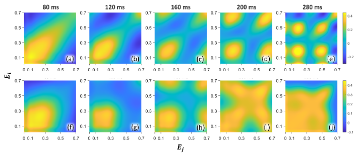
Figure 1: Correlation function c${}^{\perp}_{ij}$, ensemble-averaged over 30 shots with a selected $\varphi$ distribution , at different evolution times with interaction strength $\zeta=1.2$ (top row (a-e)) and $\zeta=1.8$ (bottom row (f-j)). Figures in the same row share the same color bar on the right. In this figure, only the lowest $70\%$ of energy bins are adopted in data analysis as higher energy groups contain very few particles. $E_{i}$ and $E_{j}$ are in units of effective Fermi energy $E_{F}$. The c${}^{\perp}_{ij}$ values shown here and correlation plots (b-d,f-g) in Fig. 2 are amplified by dividing an energy-dependent attenuation coefficient $\Gamma(E_{i}|\sigma_{E_{F}},\alpha_{r})$ arising from the finite energy resolution ($\lesssim 0.08\sqrt{E_{i}}$) to restore the amplitudes to their correct values Sup .

The first term represents the effective long-range interactions between energy lattice site $i$ and $j$ due to the overlap of probability densities in real space for the energy states $i$ and $j$. $g_{ij}(a)$ is the coupling parameter, scaling linearly with scattering length $a$. In our system, the average $g_{ij}(a)$ is $\bar{g}(a=5.2\,a_{0})\approx 1.7$ Hz $\times 2\pi$.

The second term arises from the magnetic field variation along the axial direction of the cloud, resulting in an effective spin-dependent harmonic potential. $\Omega^{\prime}=-\delta\omega_{x}/(\hbar\omega_{x})$, with $\delta\omega_{x}/2\pi=14.06$ mHz for our trap. For the mean energy $\bar{E}_{x}\simeq k_{B}T_{F}/4$, $\Omega^{\prime}\,\bar{E}_{x}\simeq 2.0$ Hz $\times 2\pi$. The statistical standard deviation of $\Omega^{\prime}\,E_{x}$ is calculated to be $\sigma_{\Omega_{z}}\approx 1.4$ Hz and determines the spread in the spin-precession rates.

The ratio of these two terms in Eq. 1 determines the behavior of the system during evolution. For this reason, we define the dimensionless interaction strength $\zeta\equiv\bar{g}(a)/(\sqrt{2}\sigma_{\Omega_{z}})$. Here, larger $\zeta$ represents a stronger mean-field interaction, and for small $\zeta$, the system is dominated by the spread in Zeeman precession.

To predict the dynamics of the system, a mean-field approximation is applied. Collective spin vectors are obtained by neglecting quantum correlations in the Heisenberg equations: $\dot{\vec{s}}_{i}(t)=\vec{\omega}_{i}(t)\times{\vec{s}}_{i}(t)$ Pegahan et al. (2019); Huang et al. (2023). The components of collective spin vector for different energy groups $s_{\sigma}(E_{i})$ are obtained by numerical integration.

To observe the transverse component of the spin vector, a Ramsey sequence is applied. Starting from an initially $z$-polarized state, the first excitation $(\frac{\pi}{2})_{y}$ RF pulse produces an $x$-polarized sample. After that, the system is allowed to evolve for a period $\tau$ at the scattering length $a$ of interest. Then, a second $(\frac{\pi}{2})_{y}$ RF pulse is applied to collectively rotate the spin vectors about the $y$-axis, projecting the $x$-component onto the measurement $z$-axis, ideally. Immediately after the last RF pulse, two spin states $|\uparrow_{z}\rangle$ and $|\downarrow_{z}\rangle$ are imaged. In reality, as discussed below, $s_{z}(x)=(n_{\uparrow}(x)-n_{\downarrow}(x))/2\equiv s^{meas}(x)$ measures a combination of transverse components of the spin vector in the Bloch resonant frame, $\tilde{s}_{x}$ and $\tilde{s}_{y}$, just prior to imaging. Abel inversion is applied to $s^{meas}(x)$ to obtain the energy-resolved spin density $s^{meas}(E)$ with a bin width of $\Delta E=E_{F}/50$ Pretzier (1991); Sup . Note that even though the energy bin size is finite, the system itself is quasi-continuous because of the large atom number and closely spaced energy levels.

During the experimental cycle, magnetic field fluctuation, at even $10^{-4}$ G level, causes imperfectly controlled RF detuning and subsequent phase $\varphi$ accumulation, changing the relative contribution of the $x$ and $y$ components of spin vectors in the measurement, $s^{meas}=\cos(\varphi)\tilde{s}_{x}+\sin(\varphi)\tilde{s}_{y}$. With a broad spread $\varphi\in[0,2\pi]$, a multi-shot average $\langle s^{meas}\rangle$ tends to vanish. As the $\varphi$ distribution for each data set is usually irreproducible, the contribution of the $x$ and $y$ components in $\langle s^{meas}\rangle$ cannot be controlled in an efficient and reliable way even with data selection Sup . This problem is circumvented in analyzing the correlation between measured operators with energy $E_{i}$ and $E_{j}$, which has the form Sup :

$$\begin{split}\mathcal{C}^{\perp}_{ij}\equiv\langle s^{meas}_{i}s^{meas}_{j}\rangle=&\frac{1}{2}\langle\tilde{s}_{xi}\tilde{s}_{xj}+\tilde{s}_{yi}\tilde{s}_{yj}\rangle\\ +&\frac{1}{2}\langle\cos(2\varphi)\rangle\langle\tilde{s}_{xi}\tilde{s}_{xj}-\tilde{s}_{yi}\tilde{s}_{yj}\rangle\\ -&\frac{1}{2}\langle\sin(2\varphi)\rangle\langle\tilde{s}_{xi}\tilde{s}_{yj}+\tilde{s}_{yi}\tilde{s}_{xj}\rangle,\end{split}$$ (2)

where $\langle\cdots\rangle$ denotes an average over multi-shots, and $\tilde{s}_{\sigma i}$ is the $\sigma$ component of spin vector in Bloch frame before the last $(\frac{\pi}{2})_{y}$ pulse. In the data analysis, a data group is selected with a specific phase distribution Sup to enforce $\langle\cos(2\varphi)\rangle=\langle\sin(2\varphi)\rangle=0$, estimated using the quasi-classical spin model. This method ensures that the correlation obtained by averaging selected single shots is $\mathcal{C}^{\perp}_{ij}=\frac{1}{2}\langle\tilde{s}_{xi}\tilde{s}_{xj}+\tilde{s}_{yi}\tilde{s}_{yj}\rangle$, without making assumptions about the $\varphi$ distribution for the whole data set.

In contrast, both $\langle\tilde{s}_{zi}\rangle$ and $\langle\tilde{s}_{zi}\tilde{s}_{zj}\rangle$ can be measured easily without data selection, as this measurement does not require the last $(\frac{\pi}{2})_{y}$ RF pulse, and therefore, is insensitive to the RF detuning. We have conducted ensemble averaged $\tilde{s}_{z}$ measurement and found that $(\langle\tilde{s}_{zi}\tilde{s}_{zj}\rangle-\langle\tilde{s}_{zi}\rangle\langle\tilde{s}_{zj}\rangle)/(N_{i}N_{j}/4)$ has a value of $\sim 5\times 10^{-3}$, which is comparable to spin projection noise, indicating the system is not quantum correlated. In addition, as our previous single-shot measurements showed, this large spin system can be well explained by a quasi-classical model Huang et al. (2023). Therefore, we expect this system evolves classically, where the classical correlation $\mathcal{C}_{ij}^{\perp}$ is of interest. By construction, $\mathcal{C}_{ij}^{\perp}$ also detects quantum correlations when they are present.

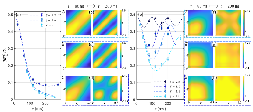
Figure 2: Time-dependent magnetization with different interaction strength and corresponding c${}_{ij}^{\perp}$ correlation plots. Blue circles in (a) and (e) are averaged data over multiple shots with desired $\varphi$ distribution. Darker blue corresponds to stronger interaction. A detailed description of data selection and error bar calculation is in Supplement Sup § A.4. Dashed lines are predictions from the quasi-classical spin model. Correlation plots (b-d) and (f-h) show c${}_{ij}^{\perp}$ at $\tau=80$ ms (left of each pair) and $200$ ms (right of each pair). (b) $\zeta=0\,(a=0\,a_{0})$, (c) $\zeta=0.6\,(a=2.62\,a_{0})$, (d) $\zeta=1.2\,(a=5.19\,a_{0})$, (f) $\zeta=1.8\,(a=8.05\,a_{0})$, (g) $\zeta=2.3\,(a=10.54\,a_{0})$, (h) $\zeta=2.9\,(a=13.20\,a_{0})$. Same as Fig. 1, only $E_{i},E_{j}\in[0,0.7]E_{F}$ are shown in these correlation plots.

Fig. 1 shows the evolution of $\mathcal{C}^{\perp}_{ij}$ with interaction strengths $\zeta=1.2$ ($a=5.19\,a_{0}$) (top row (a-e)) and $\zeta=1.8$ ($a=8.05\,a_{0}$) (bottom row (f-j)), normalized by the product of atom numbers in the corresponding energy partitions $i$ and $j$. We define c${}_{ij}^{\perp}\equiv\mathcal{C}_{ij}^{\perp}/(N_{j}N_{j}/4)$ for convenience. Therefore, each pixel represents c${}_{ij}^{\perp}$, the correlation between one pair of particles in energy groups $E_{i}$ and $E_{j}$, with maximum and minimum possible values $\pm\frac{1}{2}$ by construction from Eq. 2. It is observed that the system evolves in a qualitatively different way as the interaction strength increases. At $\zeta=1.2$, the single particle pair correlation tends to be localized between multiple specific energy subgroups. At $\zeta=1.8$, the correlation tends to become uniform across all pairs of energy groups. This qualitatively distinct behavior of microscopic correlations reveals the source of the transition in macroscopic quantities such as magnetization.

The system magnetization is related to the ensemble-averaged correlation functions by definition. The square of total transverse magnetization $\mathcal{M}_{\perp}^{2}=S_{x}^{2}+S_{y}^{2}$ is the double summation of the perpendicular correlation in energy space: $\frac{1}{2}\mathcal{M}^{2}_{\perp}=\sum_{i,j}\mathcal{C}_{ij}^{\perp}$.

Fig. 2 shows the time-evolution of $\mathcal{M}^{2}_{\perp}$ with different interaction strengths. The qualitative change in the behavior of the magnetization is also observed in the microscopic correlation c${}_{ij}^{\perp}$ between energy subgroups, which are shown as correlation plots in (b-d,f-h). For all pairs of correlation plots, the left one corresponds to $\tau=80$ ms and the right one corresponds to $\tau=200$ ms. For the lighter blue data in (a), where the interaction strength is very small $\zeta=0,\,0.6$, $\frac{1}{2}\mathcal{M}^{2}_{\perp}(t\rightarrow\infty)=0$. For the darkest blue data in (a), where $\zeta=1.2$, $\frac{1}{2}\mathcal{M}^{2}_{\perp}(t\rightarrow\infty)$ asymptotes to a non-zero, small value. For small scattering lengths, correlation figures in (b-d) show that as time evolves, the largest correlations $|$c${}_{ij}^{\perp}|$ (either positive or negative) arise between certain localized energy groups, either forming thin stripes or forming islands. Note that, with the absence of mean-field interaction, i.e., at $0\,a_{0}$, the uniform stripes shown in (b) are the Ramsey fringes in energy space. By analyzing the width of the Ramsey fringes, the Zeeman tuning rate $\Omega^{\prime}$ can be tested Sup . For stronger interactions shown in (e), where $\zeta\geq 1.8$, $\frac{1}{2}\mathcal{M}^{2}_{\perp}(t\rightarrow\infty)$ tends to oscillate relative to a larger static level as $\zeta$ increases. In addition, the behavior in pair correlation shown in (f-h) is totally different from that for small $\zeta$ (b-d). With strong interactions, high correlation regions tend to spread over all pairs of energy groups $i$ and $j$.

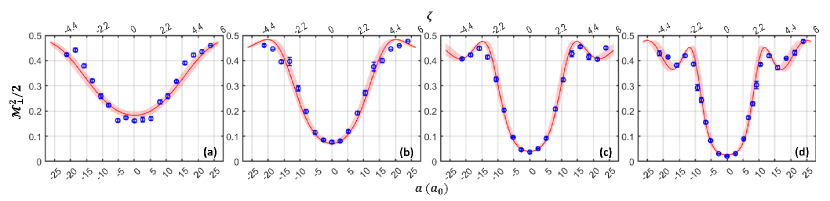
Figure 3: Observing the emergence of spin locking by measuring $\frac{1}{2}\mathcal{M}_{\perp}^{2}$ for various interaction strength $\zeta$ (top axis) and corresponding scattering lengths $a$ (bottom axis) at (a) 80 ms, (b) 120 ms, (c) 160 ms, and (d) 200 ms. Blue circles are averaged data over multiple shots with the same averaging and error bar calculation for Fig. 2. Bright red curves are predictions with the quasi-classical spin evolution model and the pink bands correspond to a $2\%$ standard deviation in cloud size $\sigma_{Fx}$.

The transition in behavior of $\frac{1}{2}\mathcal{M}_{\perp}^{2}$, which occurs between Fig. 2(a-d) and (f-h) matches the one observed between Fig. 1 top row (a-e) and bottom row (f-j). From the measured energy-space correlation function c${}_{ij}^{\perp}$, we conclude that a system with a more localized transverse correlation between multiple specific energy group pairs tends to be demagnetized as time evolves (Fig. 2(a)). In contrast, a system with the transverse correlation spread over most energy group pairs maintains the high initial magnetization (Fig. 2(e)).

Furthermore, even when $\mathcal{M}_{\perp}^{2}$ has the same value at two different times, it is observed that the corresponding correlation plots can have totally different structures. As shown in Fig. 2(e), $\mathcal{M}_{\perp}^{2}(80\,\text{ms})=\mathcal{M}_{\perp}^{2}(200\,\text{ms})$ for $\zeta=1.8$, but the corresponding c${}_{ij}^{\perp}$ (Fig. 2(f)) shows different features for these two times. Similarly, for $\zeta=1.2$ in Fig. 2(a), $\mathcal{M}_{\perp}^{2}(200\,\text{ms})=\mathcal{M}_{\perp}^{2}(280\,\text{ms})$, but Fig. 1(e)(f) show different behaviors of c${}_{ij}^{\perp}$. Therefore, the observation of energy-resolved correlation provides a new probe to characterize the spin dynamic more deeply than simply measuring macroscopic quantities.

Fig. 3 shows the emergence of $xy$-plane magnetization versus interaction strength at four evolution times. Blue circles are measured $\mathcal{M}^{2}_{\perp}$, for the same sample selection method described above. Predictions of $\mathcal{M}_{\perp}^{2}$ (red curves) are obtained using the quasi-classical model. We find that, as the interaction strength increases, $\mathcal{M}^{2}_{\perp}$ surges, simulating a transition to a ferromagnetic state.

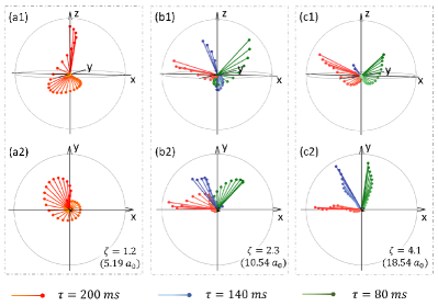
Figure 4: Modeled spin vector for different energy partitions (longer segments represent spin vectors with lower energy and vice versa). (a1,a2) are spin vectors with $\zeta=1.2$ at $200$ ms. (b1,b2,c1,c2) are spin vectors at different $\tau$ with $\zeta=2.3$ and $4.1$ respectively. (a2,b2,c2) are the top views of (a1,b1,c1). Red, blue, and green segments are spins at $200$, $140$, and $80$ ms respectively.

A sharp rise in $|\mathcal{M}_{\perp}|$ has been observed and considered as a transition between dynamical states  Smale et al. (2019). The spin vector picture provides a physical illustration of this transition. Recall that, by definition, $\mathcal{M}^{2}_{\perp}=S_{x}^{2}+S_{y}^{2}$. Thus, the magnetization is related to the dispersion of the spin vector in the $xy$-plane: the more spins cluster, the larger magnitude $\mathcal{M}^{2}_{\perp}$ has. This can be considered as a spin-locking effect. Fig. 4 depicts this phenomenon using the quasi-classical spin model. (a1,a2) shows the spin vectors with different energies after evolving for $200$ ms with a small interaction strength $\zeta=1.2$. (a2) is the top view of (a1) and clearly shows spin vectors in different energy partitions are largely spread out over all four quadrants in the $xy$-plane. In the microscopic correlation picture, spins with the same or opposite azimuthal angles are strongly correlated, and positive and negative single-pair correlations tend to cancel each other, leaving a weak magnetization after double summation over all energy partitions, corresponding to low $\mathcal{M}^{2}_{\perp}$ value in Fig. 3(d). In contrast, (c1,c2) demonstrate a spin-locked state, with $\zeta=4.1$ after evolving for 80 ms (green), 140 ms (blue), and 200 ms (red). For all three evolution times, the spin vectors in all energy partitions tend to congregate. In this situation, spins in all energy partitions are strongly and positively correlated, resulting in a highly magnetized state, in agreement with Fig. 3(a-d) for $\zeta=4.1$. (b1,b2) shows an intermediate stage between (c1,c2) and (a1,a2): the spin vectors have not formed a bundle at $\tau=80$ ms (green), but start showing this trend at $\tau=140$ ms, (blue) and $200$ ms (red). Further, as interaction strength increases, $s_{zi}$ also tends to cluster, with $\langle S_{z}^{2}\rangle$ becoming small as $\langle S_{x}^{2}+S_{y}^{2}\rangle$ increases.

In summary, we have developed energy-space spin correlation measurement as a method for characterizing the spin dynamics of quasi-continuous, weakly interacting quantum gases, which simulate a synthetic lattice of spins pinned in energy space. This method enables a full view of how correlations develop between the extensive subsets of spins in energy space on a microscopic level, associating the evolution of the macroscopic properties with the local correlation behavior. Utilizing this idea, we connect the spread and localization of correlations to the system magnetization and demagnetization by observing the correlation distribution as a function of time and interaction strength. This energy-resolved probe can be exploited in studies of macroscopic out-of-equilibrium dynamics and critical dynamics across quantum phase transitions.

We thank Ilya Arakelyan for helpful discussions. Primary support for this research is provided by the Air Force Office of Scientific Research (FA9550-22-1-0329). Additional support is provided by the National Science Foundation (PHY-2006234 and PHY-2307107).

^∗Corresponding authors: jhuang39@ncsu.edu
                                     jethoma7@ncsu.edu

Appendix A Supplemental Material

This supplemental material presents details of experimental procedures, data analysis, and modeling for measurement of transverse spin components in a weakly interacting Fermi gas. We discuss the mathematical formalism of Abel inversion and apply it to obtain the energy-resolved spin density from measurement in real space. A data selection method specific to measurement of transverse spin correlation is described and illustrated by deriving the final state of a non-interacting gas after a Ramsey sequence. Finally, an energy-dependent attenuation coefficient for the ensemble-averaged correlation, arising from the finite energy resolution, is introduced and tested on data.

A.1 Experimental procedure

The experiment presented in this work is implemented with ⁶Li atoms. A 50-50 incoherent mixture of two lowest hyperfine states $|1\rangle$ and $|2\rangle$ are evaporatively cooled in a CO₂ laser optical trap to degeneracy. Then state $|1\rangle$ is eliminated with a $17\,\mu$s imaging pulse at a magnetic field of $\sim 1200$G. With one spin state left in the sample, the magnetic field is swept close to zero-crossing (527.15 G) so that both the magnitude and sign of scattering length can be tuned during experiments. After the magnetic field is stabilized at the experimental value, an excitation RF $(\frac{\pi}{2})_{y}$ (0.5 ms), which is on resonance with $|2\rangle$ to $|1\rangle$ transition, is applied to create a $x$-polarized sample. With the coherent mixture of these two states, the system is allowed to evolve with s-wave scattering for a time period $\tau$. Then another $(\frac{\pi}{2})_{y}$ RF pulse is applied to observe the transverse components of spin vector. Immediately after the Ramsey sequence is completed, two imaging pulses separated by $10\,\mu$s are shined to the sample to obtain the absorption images of both spins. With these images, integration across the radial direction yields the axial spatial density profiles $n_{1}(x)$ and $n_{2}(x)$. With the technique of Abel inversion (introduced in §A.2), the energy space profiles $n_{1}(E)$ and $n_{2}(E)$ of the two states are obtained from the measured spatial profiles.

A.2 Abel Inversion

In this section, we introduce a numerical solution of Abel-type integral equations using an improved method that was first presented in 1991 Pretzier (1991). We apply this method to extract energy space spin densities from spatial profiles measured in the experiments presented in this work. This Abel inversion solution is obtained by expanding the energy integral in a series of cosine functions whose amplitudes are calculated by least-squares-fitting from the measured spatial data. The number of expansion terms is determined by the complexity of the data. We use 8-12 expansion terms for the data presented in this work.

A.2.1 Formalism

Abel inversion is an optimum way to evaluate the energy distribution of a given spatial profile along the longitudinal axis, although it was first designed for the extraction of a distribution in the radial direction from a measurement of distribution in the axial direction. The Abel transform has the form

$$h(y)=2\int^{R}_{y}f(r)\frac{r\,dr}{\sqrt{r^{2}-y^{2}}},$$ (S1)

where $h(y)$ is a measured physical quantity and $f(r)$ is an unknown function. To evaluate $f(r)$, it is expanded into $n_{max}$ cosine terms Pretzier (1991):

$$f(r)=\sum_{n=0}^{n_{max}}A_{n}\,f_{n}(r),$$ (S2)

$$f_{n}(r)=\left\{\begin{array}[]{lcl}0&\text{, for }n=0;\\ 1-(-1)^{n}\cos\left(n\pi\frac{r}{R}\right)&\text{, otherwise}.\end{array}\right.$$ (S3)

Using Eq. S1 and Abel transform of Eq. S2, we define $H(y)$ as a summation of $n_{max}$ terms:

$$\begin{split}H(y)=&\,2\sum_{n=0}^{n_{max}}A_{n}\int_{y}^{R}f_{n}(r)\frac{r\,dr}{\sqrt{r^{2}-y^{2}}}\\ =&\,2\sum_{n=0}^{n_{max}}A_{n}h_{n}(y)\end{split}$$ (S4)

where $y$ is the independent variable.

Assume that in each measurement, there are $k_{max}$ values of $y_{k}$ in total, forming set $Y$. Therefore, the corresponding measured value $d_{k}=h(y_{k})$ has $k_{max}$ values, too, forming set $D$:

$$\begin{split}h|_{Y}:Y\rightarrow D;\qquad&d_{k}\in D:\{k\in\mathbb{N}_{1}:\,k\leq k_{max}\}\\ &y_{k}\in Y:\{k\in\mathbb{N}_{1}:\,k\leq k_{max}\}.\end{split}$$ (S5)

In this work, the independent variable $x$ for the spatial profile $s^{meas}(x)$ is scaled by the size of the cloud $\sigma_{Fx}$ for each shot such that $x_{k}/\sigma_{Fx}\in[-1,1]$. Then the raw measured axial spatial profile $s^{meas}(x)$ is folded over the center of cloud where $x_{k}=0$, and binned into 50 points. After this process, $x_{k}/\sigma_{Fx}\in[0,1]$. It’s convenient to use: $y_{k}\rightarrow x_{k}/\sigma_{Fx}$, thus $y_{k}\in[0,1]$ and $k_{max}=50$.

With this measurement, calculate the squared difference between expansion $H(y)$ and measured $h(y)$:

$$\chi^{2} =\sum_{k}[h(y_{k})-H(y_{k})]^{2}$$

$$=\sum_{k}\left[d_{k}-\sum_{n=0}^{n_{max}}A_{n}h_{n,k}\right]^{2}$$

and minimize it by $\frac{\partial\chi^{2}}{\partial A_{n}}=0$

$$2\sum_{k}\left[d_{k}-\sum_{n=0}^{n_{max}}A_{n}h_{n,k}\right]h_{m,k}=0$$ (S6)

$$\underbrace{\sum_{k}d_{k}h_{m,k}}_{\equiv V_{m}}=\underbrace{\sum_{n}\sum_{k}h_{n,k}h_{m,k}}_{\equiv M_{mn}}A_{n}$$ (S7)

$$\Rightarrow\qquad A_{n}=(M^{-1})_{nm}V_{m}.$$ (S8)

With the values of coefficients $A_{n}$ optimized, the expansion $H(y)$ will have a numerical form.

A.2.2 Real space and energy space

To apply the Abel inversion to obtain energy profile from spatial one, the correspondence between them needs to be understood. In this section, we illustrate how to achieve the form shown in Eq. S1 with correct dimensions.

Atom density in real space and energy space is connected by the density probability function:

$$n_{\sigma}(x)=\frac{1}{\pi}\int dE\,|\phi_{E}(x)|^{2}\,n_{\sigma}(E).$$ (S9)

A WKB approximation is applied to evaluate $|\phi_{E}(x)|^{2}$:

$$|\phi_{E}(x)|^{2}\approx\frac{\Theta\left[\frac{2E}{m\omega_{x}^{2}}-x^{2}\right]}{\pi\sqrt{\frac{2E}{m\omega_{x}^{2}}-x^{2}}},$$

$$\Rightarrow n_{\sigma}(x)=\frac{1}{\pi}\int_{\frac{m\omega_{x}^{2}x^{2}}{2}}^{E_{F}}\frac{dE\,n_{\sigma}(E)}{\sqrt{\frac{2E}{m\omega_{x}^{2}}-x^{2}}},$$

where $E_{F}=\frac{1}{2}m\omega_{x}^{2}\sigma_{Fx}^{2}$ is an effective Fermi energy, and the cutoff $\sigma_{Fx}$ is obtained by fitting a zero temperature Thomas Fermi profile to the spatial density of the sample.

For convenience in the calculations, the variables are converted to dimensionless forms:

$$\tilde{E}\equiv\frac{E}{E_{F}},\qquad d\tilde{E}=\frac{dE}{E_{F}}.$$

Then the upper and lower limits of the integral become:

$$\left\{\begin{array}[]{cl}\text{upper limit }&\rightarrow 1\\ \text{lower limit }&\rightarrow\frac{m\omega_{x}^{2}x^{2}}{2}/E_{F}=\frac{x^{2}}{\sigma_{Fx}^{2}}.\end{array}\right.$$ (S10)

$$\Rightarrow n_{\sigma}(x)=\frac{1}{\pi}\int^{1}_{x^{2}/\sigma_{Fx}^{2}}\frac{d\tilde{E}\,n_{\sigma}(\tilde{E})}{\sigma_{Fx}\sqrt{\tilde{E}-\frac{x^{2}}{\sigma_{Fx}^{2}}}}.$$ (S11)

Now the spatial variable is changed to its dimensionless version:

$$\tilde{X}\equiv\frac{x}{\sigma_{Fx}}$$

$$\Rightarrow n_{\sigma}(\tilde{X})=\frac{1}{\pi\sigma_{Fx}}\int^{1}_{\tilde{X}^{2}}\frac{d\tilde{E}\,n_{\sigma}(\tilde{E})}{\sqrt{\tilde{E}-\tilde{X}^{2}}}.$$ (S12)

Eq. S12 has the same form as Eq. S1 by writting

$$\frac{r}{R}\rightarrow\sqrt{\tilde{E}},$$

and the expansion terms in Eq. S3 has the form:

$$f_{n}(\sqrt{\tilde{E}})=\left\{\begin{array}[]{lcl}0&\text{, for }n=0;\\ 1-(-1)^{n}\cos\left(n\pi\sqrt{\tilde{E}})\right)&\text{, otherwise}.\end{array}\right.$$ (S13)

$h_{n}(y)$ in Eq. S4 becomes:

$$h_{n}(\tilde{X})=\frac{1}{\sigma_{Fx}}\int^{1}_{\tilde{X}^{2}}\frac{d\tilde{E}}{\sqrt{\tilde{E}-\tilde{X}^{2}}}f_{n}(\sqrt{\tilde{E}}).$$ (S14)

Performing least-squares-fitting, as introduced in Eq. S6, with data $d_{k}=n_{\sigma}(\tilde{X}_{k})$ and Eq. S14, will yield a numerical form of $n_{\sigma}(\tilde{E})$. In this way, the spin density in energy space is obtained.

A.2.3 Energy resolution

The imaging system in our lab has a spatial resolution $\delta x\approx 5\,\mu$m. This results in a finite resolution in energy space, $\delta E_{s}$. Since the energy is related to the spatial position,

$$E=\frac{1}{2}m\omega_{x}^{2}x^{2},$$

the resolution in energy space can be estimated by:

$$\delta E_{s}\approx\delta(\frac{1}{2}m\omega_{x}^{2}x^{2})=\frac{2x\delta x}{\sigma_{x}^{2}}E_{F}\approx 0.03\,E_{F}\sqrt{\tilde{E}}\,,$$ (S15)

since $x^{2}/\sigma_{Fx}$ scales as $\sqrt{E_{i}/E_{F}}$.

Furthermore, $n_{\sigma}(\tilde{E})$ has a finite resolution in energy space, $\delta E_{A}$, which is related to the maximum number of terms, $n_{max}$, adopted in the Abel inversion. From Eq. S13, we can write the $n^{th}$ ($n>0$) expansion term as

$$f_{n}(\sqrt{\tilde{E}})=1-(-1)^{n}\cos{\phi^{\prime}_{n}(\sqrt{\tilde{E}})}\,,$$

where $\phi^{\prime}_{n}(\sqrt{\tilde{E}})\equiv n\pi\sqrt{\tilde{E}}$. Then the resolution $\delta E_{A}$ can be estimated by setting

$$\begin{split}1&\simeq\delta E_{A}\frac{\partial\phi^{\prime}_{n}(\sqrt{\tilde{E}})}{\partial E}\Bigg{\rvert}_{n=n_{max}}\\ 1&=\delta E_{A}\frac{\partial(n_{max}\pi\sqrt{E_{i}/E_{F}})}{\partial{E_{i}}}\\ \Rightarrow\delta E_{A}&=\frac{2}{n_{max}\pi}\sqrt{\frac{E_{i}}{E_{F}}}E_{F}.\end{split}$$ (S16)

In the data analysis, $n_{max}=12$ is applied to most of the data, yielding $\delta E_{A}\approx 0.06\,E_{F}\sqrt{\tilde{E}}$.

A.3 Collective Spin Vector Evolution Model

To understand the effect of the RF detuning on $s^{meas}(x)$ measurement, we derive the final state of the system after the second $(\frac{\pi}{2})_{y}$ pulse. Note that, although in the main text, the measured quantity is written as $s^{meas}(x)$, it is really the $z$-component of the spin vector at the moment the system is imaged. However, after the last $(\frac{\pi}{2})_{y}$ RF pulse, there is no evolution time before imaging. Therefore, the measured quantity contains the transverse components of the spin vector just prior to imaging. For convenience, $s^{meas}$ in the main text is written as $s_{z}$ in this section so that the rotation can be illustrated more straightforwardly in the derivation.

Prior to the pulse sequence, the optically trapped atoms are initially prepared in a $z$-polarized state,

$$|\psi_{0z}\rangle=\Pi_{i}\,|\!\!\uparrow_{zi}\rangle.$$ (S17)

Therefore, the final state after the pulse sequence is

$$|\psi_{f}\rangle=e^{-i\frac{\pi}{2}S_{y}}e^{-i\frac{H}{\hbar}\tau}\underbrace{e^{-i\frac{\pi}{2}S_{y}}|\psi_{0z}\rangle}_{|\psi_{0x}\rangle}.$$ (S18)

If include the RF detuning into the Hamiltonian, Eq. 1 in the main text has a form:

$$\frac{H}{\hbar}=\sum_{i,j\neq i}g_{ij}\vec{s}_{i}\cdot\vec{s}_{j}+\sum_{i}(\Omega^{\prime}E_{i}+\Delta(t))s_{zi},$$ (S19)

where $\Delta(t)$ represents the RF detuning rate with unknown time dependence. Keeping the detuning part separate, we define the Hamiltonian with two parts:

$$\frac{H}{\hbar}=\frac{H^{0}}{\hbar}+\Delta(t)S_{z},$$ (S20)

then $H/\hbar\tau$ becomes:

$$\frac{H}{\hbar}\tau=\frac{H^{0}}{\hbar}\tau+\int_{\tau}\Delta(t)\,dtS_{z}=\frac{H^{0}}{\hbar}\tau+\varphi S_{z},$$ (S21)

where $\varphi$ is the accumulated phase shift due to RF detuning for an evolution period $\tau$.

Then the measurement of $s_{z}$ yields:

$$\langle\psi_{f}|s_{zi}|\psi_{f}\rangle=\langle\psi_{0x}|e^{i\frac{H}{\hbar}\tau}\underbrace{e^{i\frac{\pi}{2}S_{y}}s_{zi}e^{-i\frac{\pi}{2}S_{y}}}_{s_{zi}(\frac{\pi}{2})_{y}}e^{-i\frac{H}{\hbar}\tau}|\psi_{0x}\rangle.$$ (S22)

With Heisenberg equation of motion, $s^{\prime\prime}_{zi}(\theta_{y})=s_{zi}(\theta_{y})$ and initial conditions $s_{zi}(0_{y})=s_{zi}$ and $s_{zi}^{\prime}(0_{y})=-s_{xi}$, we obtain the analytic form:

$$s_{zi}(\theta_{y})=\cos(\theta_{y})s_{zi}-\sin(\theta_{y})s_{xi}.$$ (S23)

Then

$$\langle\psi_{f}|s_{zi}|\psi_{f}\rangle =\langle\psi_{0x}|e^{i\frac{H}{\hbar}\tau}(-s_{xi})e^{-i\frac{H}{\hbar}\tau}|\psi_{0x}\rangle$$

$$=\langle\psi_{0x}|e^{i\frac{H^{0}}{\hbar}\tau}e^{i\varphi S_{z}}(-s_{xi})e^{-i\frac{H^{0}}{\hbar}\tau}e^{-i\varphi S_{z}}|\psi_{0x}\rangle.$$

Since the commutation rule $[H^{0},S_{z}]=0$, rearrange the terms to get:

$$\langle\psi_{f}|s_{zi}|\psi_{f}\rangle=\langle\psi_{0x}|e^{i\frac{H^{0}}{\hbar}\tau}e^{i\varphi S_{z}}(-s_{xi})e^{-i\varphi S_{z}}e^{-i\frac{H^{0}}{\hbar}\tau}|\psi_{0x}\rangle.$$ (S24)

Similar to Eq. S23, we can derive

$$s_{xi}(\theta_{z})\equiv e^{i\theta S_{z}}s_{xi}e^{-i\theta S_{z}}=\cos(\theta_{z})s_{xi}-\sin(\theta_{z})s_{yi}.$$ (S25)

Then the measurement of $s_{zi}$ becomes:

$$\langle\psi_{f}|s_{zi}|\psi_{f}\rangle=\langle\psi_{0x}|e^{i\frac{H^{0}}{\hbar}\tau}(s_{xi}\cos\varphi-s_{yi}\sin\varphi)e^{-i\frac{H^{0}}{\hbar}\tau}|\psi_{0x}\rangle.$$ (S26)

For convenience, define:

$$\tilde{s}_{\sigma i}=e^{i\frac{H^{0}}{\hbar}\tau}s_{\sigma i}e^{-i\frac{H^{0}}{\hbar}\tau},$$

then

$$\langle\psi_{f}|s_{zi}|\psi_{f}\rangle=\langle\psi_{0x}|(\tilde{s}_{xi}\cos\varphi-\tilde{s}_{yi}\sin\varphi)|\psi_{0x}\rangle.$$ (S27)

To calculate the correlation, start from:

$$\langle\psi_{f}|s_{zi}s_{zj}|\psi_{f}\rangle=\langle\psi_{0x}|e^{i\frac{H}{\hbar}\tau}\underbrace{e^{i\frac{\pi}{2}S_{y}}s_{zi}s_{zj}e^{-i\frac{\pi}{2}S_{y}}}_{(*)}e^{-i\frac{H}{\hbar}\tau}|\psi_{0x}\rangle.$$ (S28)

Inserting identity operator $\mathbb{I}$:

$$(*)=e^{i\frac{\pi}{2}S_{y}}s_{zi}s_{zj}e^{-i\frac{\pi}{2}S_{y}}=e^{i\frac{\pi}{2}S_{y}}s_{zi}e^{-i\frac{\pi}{2}S_{y}}e^{i\frac{\pi}{2}S_{y}}s_{zj}e^{-i\frac{\pi}{2}S_{y}}.$$

Using Eq. S23 again:

$$(*)=s_{xi}s_{xj}.$$

Then Eq. S28 becomes:

$$\langle\psi_{f}|s_{zi}s_{zj}|\psi_{f}\rangle =\langle\psi_{0x}|e^{i\frac{H}{\hbar}\tau}s_{xi}s_{xj}e^{-i\frac{H}{\hbar}\tau}|\psi_{0x}\rangle$$

$$=\langle\psi_{0x}|e^{i\frac{H^{0}}{\hbar}\tau}e^{i\varphi S_{z}}s_{xi}s_{xj}e^{-i\frac{H^{0}}{\hbar}\tau}e^{-i\varphi S_{z}}|\psi_{0x}\rangle.$$

Exchange $H^{0}$ and $S_{z}$ terms and inserting $\mathbb{I}$ again:

$$\langle\psi_{f}|s_{zi}s_{zj}|\psi_{f}\rangle=\langle\psi_{0x}|e^{i\frac{H^{0}}{\hbar}\tau}\underbrace{e^{i\varphi S_{z}}s_{xi}e^{-i\varphi S_{z}}}_{(*1)}\underbrace{e^{i\varphi S_{z}}s_{xj}e^{-i\varphi S_{z}}}_{(*2)}e^{-i\frac{H^{0}}{\hbar}\tau}|\psi_{0x}\rangle.$$ (S29)

Evaluating $(*1)$ and $(*2)$ with Eq. S25 again, we obtain:

$$\langle\psi_{f}|s_{zi}s_{zj}|\psi_{f}\rangle=\langle\psi_{0x}|e^{i\frac{H^{0}}{\hbar}\tau}(s_{xi}\cos\varphi-s_{yi}\sin\varphi)(s_{xj}\cos\varphi-s_{yj}\sin\varphi)e^{-i\frac{H^{0}}{\hbar}\tau}|\psi_{0x}\rangle.$$ (S30)

Using trigonometry and rearranging terms, the correlation has the form:

$$\Rightarrow\mathcal{C}_{ij}^{\perp}\equiv\langle\psi_{f}|s_{zi}s_{zj}|\psi_{f}\rangle =\frac{1}{2}\langle\psi_{0x}|\tilde{s}_{xi}\tilde{s}_{xj}+\tilde{s}_{yi}\tilde{s}_{yj}|\psi_{0x}\rangle$$

$$+\frac{1}{2}\langle\cos(2\varphi)\rangle\langle\psi_{0x}|\tilde{s}_{xi}\tilde{s}_{xj}-\tilde{s}_{yi}\tilde{s}_{yj}|\psi_{0x}\rangle$$ (S31)

$$-\frac{1}{2}\langle\sin(2\varphi)\rangle\langle\psi_{0x}|\tilde{s}_{xi}\tilde{s}_{yj}+\tilde{s}_{yi}\tilde{s}_{xj}|\psi_{0x}\rangle.$$

A.3.1 Zero scattering length limit

At the magnetic field where the scattering length vanishes, the spin vector evolution is independent of the mean-field interaction: the system evolves under Zeemen precession only. In this section, we derive the prediction for the measured ensemble averaged transverse components of the spin vector and their correlation at $0\,a_{0}$, including an uncontrolled detuning. In this case,

$$\frac{H^{0}}{\hbar}\tau=\sum_{i}\vartheta_{Ei}s_{zi},$$ (S32)

$$\text{where }\,\vartheta_{Ei}\equiv\Omega^{\prime}E_{i}\tau=-\frac{\delta\omega_{x}}{\hbar\overline{\omega}_{x}}\tau\frac{E_{i}}{E_{F}}E_{F}.$$ (S33)

$\vartheta_{Ei}$ is energy dependent, and directly proportional to the evolution time $\tau$. Calculating the correlation with Eq. A.3 requires all three components, which are evaluated silimarly to Eq. S25:

$$e^{i\frac{H^{0}}{\hbar}\tau}s_{xi}s_{xj}e^{-i\frac{H^{0}}{\hbar}\tau} =e^{i\frac{H^{0}}{\hbar}\tau}s_{xi}e^{-i\frac{H^{0}}{\hbar}\tau}e^{i\frac{H^{0}}{\hbar}\tau}s_{xj}e^{-i\frac{H^{0}}{\hbar}\tau}$$

$$=[s_{xi}\cos(\vartheta_{Ei})-s_{yi}\sin(\vartheta_{Ei})][s_{xj}\cos(\vartheta_{Ej})-s_{yj}\sin(\vartheta_{Ej})]$$

$$e^{i\frac{H^{0}}{\hbar}\tau}s_{yi}s_{yj}e^{-i\frac{H^{0}}{\hbar}\tau} =e^{i\frac{H^{0}}{\hbar}\tau}s_{yi}e^{-i\frac{H^{0}}{\hbar}\tau}e^{i\frac{H^{0}}{\hbar}\tau}s_{yj}e^{-i\frac{H^{0}}{\hbar}\tau}$$ (S34)

$$=[s_{yi}\cos(\vartheta_{Ei})+s_{xi}\sin(\vartheta_{Ei})][s_{yj}\cos(\vartheta_{Ej})+s_{xj}\sin(\vartheta_{Ej})]$$

$$e^{i\frac{H^{0}}{\hbar}\tau}s_{xi}s_{yj}e^{-i\frac{H^{0}}{\hbar}\tau} =e^{i\frac{H^{0}}{\hbar}\tau}s_{xi}e^{-i\frac{H^{0}}{\hbar}\tau}e^{i\frac{H^{0}}{\hbar}\tau}s_{yj}e^{-i\frac{H^{0}}{\hbar}\tau}$$

$$=[s_{xi}\cos(\vartheta_{Ei})-s_{yi}\sin(\vartheta_{Ei})][s_{yj}\cos(\vartheta_{Ej})+s_{xj}\sin(\vartheta_{Ej})]\,.$$

Then with some trigonometry:

$$e^{i\frac{H^{0}}{\hbar}\tau}(s_{xi}s_{xj}+s_{yi}s_{yj})e^{-i\frac{H^{0}}{\hbar}\tau}= \,\cos(\vartheta_{Ej}-\vartheta_{Ei})(s_{xi}s_{xj}+s_{yi}s_{yj})$$

$$+\sin(\vartheta_{Ej}-\vartheta_{Ei})(s_{yi}s_{xj}-s_{xi}s_{yj})$$

$$e^{i\frac{H^{0}}{\hbar}\tau}(s_{i}s_{xj}-s_{yi}s_{yj})e^{-i\frac{H^{0}}{\hbar}\tau}= \,\cos(\vartheta_{Ej}+\vartheta_{Ei})(s_{xi}s_{xj}+s_{yi}s_{yj})$$ (S35)

$$-\sin(\vartheta_{Ej}+\vartheta_{Ei})(s_{yi}s_{xj}+s_{xi}s_{yj})$$

$$e^{i\frac{H^{0}}{\hbar}\tau}(s_{xi}s_{yj}+s_{xj}s_{yi})e^{-i\frac{H^{0}}{\hbar}\tau}= \,\cos(\vartheta_{Ej}+\vartheta_{Ei})(s_{xi}s_{yj}+s_{yi}s_{xj})$$

$$+\sin(\vartheta_{Ej}+\vartheta_{Ei})(s_{xi}s_{xj}-s_{yi}s_{yj})\,.$$

Since $s_{xi}|\uparrow_{xi}\rangle=N_{i}/2|\uparrow_{xi}\rangle$,

$$\langle\psi_{0x}|s_{xi}s_{xj}|\psi_{0x}\rangle=\frac{N_{i}}{2}\frac{N_{j}}{2}.$$

When $i=j$, $\langle s_{xi}s_{yj}\rangle<<N_{i}^{2}/4$ for $N_{i}>>1$. For $i\neq j$,

$$\langle\psi_{0x}|s_{yi}s_{xj}|\psi_{0x}\rangle=\langle\psi_{0x}|s_{xi}s_{yj}|\psi_{0x}\rangle=0.$$

Using these results, Eq. A.3 can be simplified and the correlation can be written as:

$$\textit{{c}}_{ij}^{\perp}\equiv\frac{\langle\psi_{f}|s_{zi}s_{zj}|\psi_{f}\rangle}{N_{i}N_{j}/4} =\frac{1}{2}\cos(\vartheta_{Ej}-\vartheta_{Ei})$$

$$+\frac{1}{2}\langle\cos(2\varphi)\rangle\cos(\vartheta_{Ej}+\vartheta_{Ei})$$ (S36)

$$-\frac{1}{2}\langle\sin(2\varphi)\rangle\sin(\vartheta_{Ej}+\vartheta_{Ei}).$$

A.4 Data selection

Because of the unknown distribution of $\varphi$, $\langle\cos(2\varphi)\rangle$ and $\langle\sin(2\varphi)\rangle$ in Eq. A.3 can vary, leading to unknown fractions of $\tilde{s}_{x}\tilde{s}_{x}$, $\tilde{s}_{y}\tilde{s}_{y}$, and $\tilde{s}_{x}\tilde{s}_{y}$ contributions. However, by intentionally manipulating the distribution of $\varphi$ such that $\langle\cos(2\varphi)\rangle=\langle\sin(2\varphi)\rangle=0$, the measurement result is expected to give the desired $\langle\tilde{s}_{x}\tilde{s}_{x}+\tilde{s}_{y}\tilde{s}_{y}\rangle$ correlation.

A data set with the desired $\varphi$ distribution is obtained by data selection. After collecting raw data set with a number of $s^{meas}(x)$ profiles and converting them to $s^{meas}(E)$ profiles using Abel inversion, each $s^{meas}(E)$ is fit with the quasi-classical model to determine fitted $\varphi$ for each shot. Then a collection of pairs of shots are selected from the raw data set, such that in this collection, for each single shot $k$ whose fitted phase is $\varphi^{k}$, there is another unique single shot $k^{\prime}$ whose fitted phase $\varphi^{k^{\prime}}=\varphi^{k}+\frac{\pi}{2}$. $k^{th}$ and $k^{\prime th}$ shots form a data pair that makes $\langle\cos(2\varphi)\rangle=\langle\sin(2\varphi)\rangle=0$. In this way, for the whole collection of $k$ and $k^{\prime}$, we obtain $k_{max}$ pairs of single shots and $\langle\cos(2\varphi)\rangle=\langle\sin(2\varphi)\rangle=0$ is guaranteed for the selected $2k_{max}$ shots. Fig. S1 shows two examples of histograms of fitted $\varphi$, $\langle\cos(2\varphi)\rangle$ and $\langle\sin(2\varphi)\rangle$ for the raw data set (red, top row) and for the corresponding subset after data selection (blue, bottom row). For the raw data set, the distributions of these $\varphi$-related quantities are pretty random. After the data selection, $\langle\cos(2\varphi)\rangle$ and $\langle\sin(2\varphi)\rangle$ can be constrained to 0.

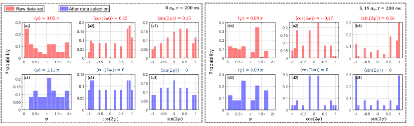
Figure S1: Histograms to show examples of distributions of $\varphi$-related quantities before (red) and after (blue) phase selection. (a1,b1,c1) shows the distribution of $\varphi$. (a2,b2,c2) shows the distribution of $\langle\cos(2\varphi)\rangle$. (a3,b3,c3) shows the distribution of $\langle\sin(2\varphi)\rangle$. Left dashed box is for [$0\,a_{0},\tau=200$ ms] data set, while right dashed box is for [$5.19\,a_{0},\tau=280$ ms].

With this method, for nonzero scattering length, the measured correlation Eq. A.3 is written as:

$$\begin{split}\mathcal{C}_{ij}^{\perp}&=\frac{1}{2}\langle\psi_{0x}|\tilde{s}_{xi}\tilde{s}_{xj}+\tilde{s}_{yi}\tilde{s}_{yj}|\psi_{0x}\rangle\\ \Rightarrow\textit{{c}}_{ij}^{\perp}&=\frac{4}{N_{i}N_{j}}\frac{1}{2}\langle\psi_{0x}|\tilde{s}_{xi}\tilde{s}_{xj}+\tilde{s}_{yi}\tilde{s}_{yj}|\psi_{0x}\rangle.\end{split}$$ (S37)

For zero scattering length, the measured correlation Eq. A.3.1 takes the form:

$$\textit{{c}}_{ij}^{\perp}=\frac{1}{2}\cos(\vartheta_{Ej}-\vartheta_{Ei})$$ (S38)

This data selection method is applied to every data set presented in this work. Each data point $\mathcal{M}_{\perp}^{2}(a,\tau)$ and its error bar in Fig. 2 and 3 are calculated from $k_{max}$ pairs of single shots. First, we make sure $k_{max}$ adopted to calculate error bar is the same for all data sets with [$a,\tau$]. Then to do data selection for each set, we randomly choose 3 pairs of $k$ and $k^{\prime}$ shots 10 times to obtain 10 $\mathcal{M}_{\perp,k}^{2}$ values. In the end, we average these 10 $\mathcal{M}_{\perp,k}^{2}$ values to obtain the ensemble-averaged macroscopic magnetization $\mathcal{M}_{\perp}^{2}$. Error bars are calculated by doing statistical standard deviation of these 10 $\mathcal{M}_{\perp,k}^{2}$ values.

Note that instead of selecting a phase $\varphi$ to be around a specific value (like maximum likelihood estimation), the method presented here enforces a distribution that is flexible, as it employs the mean and deviation of $\varphi$ for the raw data set, resulting in larger fraction of usable data. This method is also tolerant of the fitting model: as long as the fitting model can fit the data qualitatively and includes $\varphi$-dependence correctly, the selected data pairs will have the correct $\varphi_{k}^{\prime}=\varphi_{k}+\frac{\pi}{2}$, ensuring an equal distribution of $\langle s_{xi}s_{xj}\rangle$ and $\langle s_{yi}s_{yj}\rangle$ in $\langle s^{meas}_{i}s^{meas}_{j}\rangle$. If the fitting model has a systematic offset $\delta$ in fitting result $\varphi_{k}$ from the real RF detuning $\varphi_{k}^{RF}$, i.e., $\varphi_{k}=\varphi_{k}^{RF}+\delta$, this data selection method, which enforces $\varphi_{k}^{\prime}=\varphi_{k}+\frac{\pi}{2}$, will still give selected data pairs with $\varphi_{k}^{RF^{\prime}}+\delta=\varphi_{k}^{RF}+\delta+\frac{\pi}{2}$, and therefore $\varphi^{RF^{\prime}}_{k}=\varphi_{k}^{RF}+\frac{\pi}{2}$, the desired distribution.

In contrast, for $\langle s_{i}^{meas}\rangle$, data selection can only be done reliably by choosing single shots with $\varphi=0$ mod $\pi$ (ensuring $\langle s^{meas}\rangle=\pm\langle\tilde{s}_{x}\rangle$) or $\varphi=\frac{\pi}{2}$ mod $\pi$ (ensuring $\langle s^{meas}\rangle=\pm\langle\tilde{s}_{y}\rangle$). This is inefficient as the selected subset is naturally much smaller than enforcing the distribution as proposed before. Also, the data selection method enforcing a specific $\varphi$ value is highly dependent on the accuracy of fitting model. If the fitting result ends up with a systematic deviation from the real RF phase shift, then the ensemble average of the whole selected data set will have a contribution of the undesired transverse component. Therefore, $\langle\tilde{s}_{x}\rangle$ or $\langle\tilde{s}_{y}\rangle$ are not readily obtained by this method.

A.5 Energy dependent suppression

For the experiments presented in this work, the sample is destroyed upon imaging for each shot. Hence all data have slightly varying atom number and cloud size and, therefore, different Fermi energies $E_{F}$, which determines the maximum Zeeman tuning and the mean-field frequency. The correlation between different energy partitions is presented in units of $E_{F}$, and higher energy partitions are more sensitive to the variation in $E_{F}$. In addition, within one shot, there is uncertainty in the measurement of each energy partition $E_{i}$. This effect arises from the finite energy resolution of the Abel Inversion and spatial resolution of the imaging system. Therefore, after averaging over multiple shots, the magnitude of the measured correlation is suppressed more for higher energy groups.

To calculate this suppression, we use a normal distribution of $E_{F}$ and $E_{i}$:

$$P(E_{F}|\sigma_{E_{F}},\mu_{E_{F}})=\frac{1}{\sigma_{E_{F}}\sqrt{2\pi}}exp\left[-\frac{1}{2}\left(\frac{E_{F}-\mu_{E_{F}}}{\sigma_{E_{F}}}\right)^{2}\right];$$

$$P(E_{i}|\sigma_{E_{i}},\mu_{E_{i}})=\frac{1}{\sigma_{E_{i}}\sqrt{2\pi}}exp\left[-\frac{1}{2}\left(\frac{E_{i}-\mu_{E_{i}}}{\sigma_{E_{i}}}\right)^{2}\right].$$

Thus, when using Eq. S38 for $0\,a_{0}$ to estimate the suppression coefficient, the measured correlation has the form:

$$\int_{-\infty}^{\infty}dE_{F}P(E_{F}|\sigma_{E_{F}},\mu_{E_{F}})\int_{-\infty}^{\infty}dE_{i}P(E_{i}|\sigma_{E_{i}},\mu_{E_{i}})\int_{-\infty}^{\infty}dE_{j}P(E_{j}|\sigma_{E_{j}},\mu_{E_{j}})\frac{1}{2}\cos(\vartheta_{Ej}-\vartheta_{Ei})$$ (S39)

$$\textit{{c}}_{ij}^{\perp}\Rightarrow exp\left[-\frac{1}{2}\left(\Omega^{\prime}\mu_{E_{F}}\tau\right)^{2}\left[\left(\frac{\sigma_{E_{F}}}{\mu_{E_{F}}}\right)^{2}\left(\frac{E_{i}}{E_{F}}-\frac{E_{j}}{E_{F}}\right)^{2}+\alpha_{r}^{2}\left(\frac{E_{i}}{E_{F}}+\frac{E_{j}}{E_{F}}\right)\right]\right]\textit{{c}}_{ij}^{\perp}.$$

This defines an energy-dependent decay factor:

$$\Gamma(E_{i}|\sigma_{E_{F}},\alpha_{r})\equiv exp\left[-\frac{1}{2}\left(\Omega^{\prime}\mu_{E_{F}}\tau\right)^{2}\left[\left(\frac{\sigma_{E_{F}}}{\mu_{E_{F}}}\right)^{2}\left(\frac{E_{i}}{E_{F}}-\frac{E_{j}}{E_{F}}\right)^{2}+\alpha_{r}^{2}\left(\frac{E_{i}}{E_{F}}+\frac{E_{j}}{E_{F}}\right)\right]\right].$$ (S40)

The standard deviation, $\sigma_{E_{F}}$, and mean, $\mu_{E_{F}}$, of the Fermi energy $E_{F}$ are directly extracted from each data set: we calculate $E_{F}$ for all single shot data from the measured cloud size, $E_{F}=m\overline{\omega}_{x}^{2}\sigma_{Fx}^{2}/2$, and fit the distribution with a normal probability density function $P(E_{F}|\sigma_{E_{F}},\mu_{E_{F}})$. Typically, for each data set, $\sigma_{E_{F}}\approx 0.043\mu_{E_{F}}$.

$\mu_{E_{i}}$ is just the mean energy for each energy bin. $\sigma_{E_{i}}\equiv\alpha_{r}E_{F}\sqrt{E_{i}/E_{F}}$ where $\alpha_{r}$ is found from the energy uncertainty $\delta E_{A}+\delta E_{s}$. $\delta E_{A}$ arises from the number of terms $n_{max}$ adopted to apply Abel inversion as estimated in Eq. S16, $\delta E_{A}\lesssim 0.06\,E_{F}\sqrt{E_{i}/E_{F}}$ for $n_{max}=12$. $\delta E_{s}$ arises from the finite imaging resolution and is estimated in Eq. S15: $\delta E_{s}\lesssim 0.03\,E_{F}\sqrt{E_{i}/E_{F}}$. Therefore, the maximum $\alpha_{r}\approx 0.09$. In data fitting, the value of $\alpha_{r}$ is adjusted between 0.06 and 0.09, but for most cases, 0.08 is adopted.

Then the measured correlation after ensemble averaging is predicted to be scaled by $\Gamma$:

$$\Gamma(E_{i}|\sigma_{E_{F}},\alpha_{r})\,\textit{{c}}_{ij}^{\perp},$$ (S41)

with c${}_{ij}^{\perp}$ being the correct correlation between group $i$ and $j$.

A.5.1 Testing $\Gamma(E_{i}|\sigma_{E_{F}},\,\alpha_{r})$

With the parameters $\sigma_{E_{F}}$ and $\alpha_{r}$ estimated, $\Gamma(E_{i}|\sigma_{E_{F}},\,\alpha_{r})$ can be calculated and examined quantitatively by comparing the data to quasi-classical model prediction with $\Gamma$ included. Since the lowest energy group always has the largest atom number, providing the largest signal, we calculate the correlation between particles in the first (lowest) energy group and in all other energy groups, c${}_{ij}^{\perp}$, to test the validity of suppression coefficient $\Gamma(E_{i}|\sigma_{E_{F}},\,\alpha_{r})$.

The first test is implemented at zero scattering length. In this case, there is no mean-field interaction. Therefore the model prediction is very reliable as there is no approximation in the Zeeman precession term. Fig. S2 shows the result for zero scattering length case. Blue circles are the correlations obtained by averaging over about 30 single-shot data. Black dashed curves are the exact solutions predicted by Eq. S38. Note that this curve has a sinusoidal shape and the oscillation amplitude stays the same as it goes from low to high energy groups, while the data only has the same amplitude as the model at lower energy groups and becomes smaller and smaller compared to the model for higher energy groups. Red curves show the $\Gamma$ scaled model, Eq. S41. As shown in this figure, with the variation in $E_{F}$ and energy resolution included, the model and data are in quantitative agreement. The oscillation frequency of the data, which is determined by $\vartheta_{Ei}$ defined in Eq. S33, is in agreement with both predictions. This confirms that the numerical value of $\Omega^{\prime}$ adopted in our model is correct.

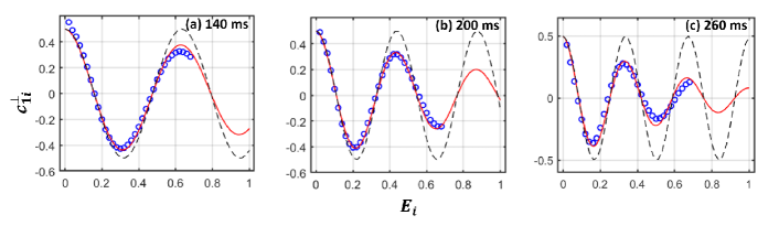
Figure S2: Comparing model with suppression factor $\Gamma$ (red curve) and without (black dashed curve) and experimental data (blue circles) for the normalized correlation c${}_{1j}^{\perp}$ at different evolution times at the zero-crossing magnetic field. Blue circles are obtained by averaging over 30 single shot data. Black dashed curve is the exact solution given in Eq. S38. Red curve is the adjusted model, which includes the shot-to-shot variation in $E_{F}$ and the finite energy resolution. In this figure, only the lowest $70\%$ energy bins are adopted in data analysis.

Fig. S3 visualizes the correlation between all energy partitions c${}_{ij}^{\perp}$ to compare model and data. The top row shows data and bottom row shows the model calculated with Eq. S41. This figure confirms the agreement between the adjusted model and data.

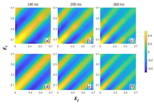
Figure S3: Normalized correlation c${}_{ij}^{\perp}$ at different evolution times at $0\,a_{0}$. Top row is calculated from data. Bottom row is predicted by the model using Eq. S38 and Eq. S41. All panels share the same color bar. In this figure, only the lowest $70\%$ of the energy bins are adopted in data analysis.

The agreement between the model with $\Gamma(E_{i}|\sigma_{E_{F}},\alpha_{r})$ included and data for the experiment conducted at the zero-crossing suggests that the calculated energy-dependent suppression coefficient $\Gamma$ predicts the decay in correlation because of the multi-shot average and finite energy resolution. To consolidate this idea and apply it to all data analysis, we do the same comparison with the data obtained at nonzero scattering length, $5.19\,a_{0}$. In such a situation, the exact solution Eq. S38 is not valid anymore. To predict the correlation, modeling $\tilde{s}_{xi}$ and $\tilde{s}_{yi}$ is required. We extract the experimental parameters $\sigma_{Fx}$ and $N$ from each shot to estimate $\tilde{s}_{xi}$ and $\tilde{s}_{yi}$ with the quasi-classical spin model, then calculate $\tilde{s}_{xi}\tilde{s}_{xj}$ and $\tilde{s}_{yi}\tilde{s}_{yj}$. Thus $\langle\psi_{0x}|\tilde{s}_{xi}\tilde{s}_{xj}|\psi_{0x}\rangle$ and $\langle\psi_{0x}|\tilde{s}_{yi}\tilde{s}_{yj}|\psi_{0x}\rangle$ are obtained by averaging over multiple predictions and c${}_{ij}^{\perp}$ is predicted using Eq. A.3.

The model in Eq. A.3 is not written in terms of $E_{F}$ or $E_{i}$ explicitly, so it is harder to include shot-to-shot variation in $E_{F}$ and finite resolution of $E_{i}$ in the model rigorously. However, a rough estimation can be made by applying the same exponential decay factor in Eq. S40 to Eq. S37. Thus, after the data selection, the measured correlation is predicted with:

$$\Gamma(E_{i}|\sigma_{E_{F}},\alpha_{r})\frac{1}{2}\langle\psi_{0x}|\tilde{s}_{xi}\tilde{s}_{xj}+\tilde{s}_{yi}\tilde{s}_{yj}|\psi_{0x}\rangle.$$ (S42)

$\mu_{E_{F}}$ and $\sigma_{E_{F}}$ are obtained by fitting normal probability density function to $E_{F}$ distribution for each data set. $\alpha_{r}$ is the same value as calculated for $0\,a_{0}$ case: $\alpha_{r}=0.09$. The result of correlation between first and all other energy groups predicted by this adjusted model is shown in red curves in Fig. S4. In this figure, blue circles are data, black dashed curves are the raw model without $E_{F}$ variation and finite energy resolution. The agreement between data and the raw model is qualitative: the oscillation frequencies of correlation for the data and model are the same, but the amplitude of correlation calculated from data is obviously smaller than the raw model prediction. In contrast, the model including $E_{F}$ variation and $E_{i}$ uncertainty fits the data much better.

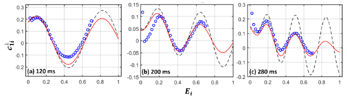
Figure S4: Comparing model with suppression factor $\Gamma$ (red curve) and without (black dashed curve) and experimental data (blue circles) for the normalized correlation c${}_{1j}^{\perp}$ at different evolution times at $5.19\,a_{0}$. Blue circles are obtained by averaging over 30 single shot data. Black dashed curve is the exact solution given in Eq. S37. Red curve is the adjusted model, which includes the shot-to-shot variation in $E_{F}$ and the finite energy resolution. In this figure, only the lowest $70\%$ energy bins are adopted in data analysis.

By comparing the ensemble-averaged c${}_{ij}^{\perp}$ over the data set after data selection to the quasi-classical model with an energy-dependent coefficient $\Gamma(E_{i}|\sigma_{E_{F}},\alpha_{r})$ included, we confirm that the numerical implementation of $\Gamma(E_{i}|\sigma_{E_{F}},\alpha_{r})$ is consistent with data as described in this section. Therefore, for all c${}_{ij}^{\perp}$ plots presented in this work, the calculated c${}_{ij}^{\perp}$ is shown after being multiplied by $\Gamma^{-1}(E_{i}|\sigma_{E_{F}},\alpha_{r})$ to restore the suppressed signal to the correct multi-shot average. The value of $\alpha_{r}$ adopted varies from 0.06 to 0.09 for fitting purposes. Note that, in $\mathcal{M}_{\perp}^{2}$ calculation, $\Gamma^{-1}(E_{i}|\sigma_{E_{F}},\alpha_{r})$ is not needed since the double summation $\sum_{i,j}\mathcal{C}_{ij}^{\perp}$ is implemented for every single shot, avoiding the suppression because of average. In the end, the $\mathcal{M}_{\perp}^{2}$ for the selected data set is obtained by averaging over that for all single shots.