Frequency Convergence of Complexon Shift Operators (Extended Version)

Abstract

Topological signal processing (TSP) utilizes simplicial complexes to model structures with higher order than vertices and edges. In this paper, we study the transferability of TSP via a generalized higher-order version of graphon, known as complexon. We recall the notion of a complexon as the limit of a simplicial complex sequence [1]. Inspired by the integral operator form of graphon shift operators, we construct a marginal complexon and complexon shift operator (CSO) according to components of all possible dimensions from the complexon. We investigate the CSO’s eigenvalues and eigenvectors, and relate them to a new family of weighted adjacency matrices. We prove that when a simplicial complex sequence converges to a complexon, the eigenvalues of the corresponding CSOs converge to that of the limit complexon. This conclusion is further verified by a numerical experiment. These results hint at learning transferability on large simplicial complexes or simplicial complex sequences, which generalize the graphon signal processing framework.

Index Terms—  Complexon, marginal complexon, shift operator, eigenvalues

1 Introduction

Graph signal processing (GSP) offers powerful tools for modeling signals associated with graph structures[2]. When presented with a fixed graph framework, one can design graph filters[3, 4] and graph neural networks[5, 6] tailored for diverse tasks, including regression and classification[7, 8], in which the eigendecomposition of the graph filter graph shift operator (GSO) plays a pivotal role[9]. There are mainly two extensions for GSP , one from the aspect of higher-order geometric structures[10] and another from the aspect of asymptotic analysis[11].

The first extension addresses the limitation of a graph structure[10]. Since a graph only captures information on nodes and edges, it cannot represent higher-order relationships between multiple nodes. One approach is to use hypergraphs to model the higher-order relationships [12, 13]. However, in some cases, signals are embedded in a specific topological structure, such as a manifold[14]. A simplicial complex[15] becomes a more appropriate model, since it can represent data on a structure with the help of homology. To develop simplicial complex signal processing (SCSP) , Hodge Laplacians are the major components to be used to derive generalized Laplacians[16] as suitable shift operators.

However, even with the first extension, the dynamic and large-scale structures encountered in signal processing turn out to be a problem. As for standard GSP and SCSP , the topological structure is assumed to be fixed. When the structure itself varies, signal processing elements like shift operators, filters, and Fourier transforms, also change. Besides, signal processing techniques such as Fourier transform are usually prohibitively expensive on large graphs or simplicial complexes.

Hence, the second extension explores the limit structure of signal processing in order to deal with the dynamic and large-scale structures. The papers [17, 18] utilize graphon to study the transferability of graph filters. Graphon signal processing tools such as graphon shift operators and graphon Fourier transforms are introduced to investigate the transferability of a graphon as the limit of a graph sequence. Analogous to a graphon, a complexon is defined as the limit of simplicial complexes and the sampling of large simplicial complex structures [1]. However, signal processing tools for complexons are yet to be developed.

In this work, we propose a novel framework called complexon shift operator (CSO) . We derive its transferability properties, as a limit theory of simplicial complexes. Such a theory paves the way for complexon-based signal processing, making it a viable tool for analyzing signals on large and dynamic simplicial complex structures. Our main contributions are summarized as follows:

• We propose the concept of a CSO for complexons, analogous to the graphon shift operator for graphons.

• We propose the raised adjacency matrix for simplicial complex and investigate its relation to the CSO of its induced complexon.

• We derive the transferability properties of the CSO and use a numerical experiment to verify it.

The rest of the paper is organized as follows. In Section 2, we briefly introduce the main concepts of GSP , graphon, and simplicial complex. In Section 3, we present the concepts and properties of complexons, and define CSO as a marginal complexon. In Section 4, we introduce the concept of a raised adjacency matrix for simplicial complex and relate it to CSO . Then we show that the eigenvalues of a simplicial complex sequence converges to that of the limit CSO . Finally, we conduct a numerical experiment to illustrate the eigenvalue convergence.

2 Preliminaries

In this section, we review the basic concepts of GSP , graphons, and simplicial complexes, which are fundamental TSP components used in setting up the theory of complexon signal processing.

2.1 Graph And Its Shift Operators

A graph $G=(\mathcal{V}(G),\mathcal{E}(G))$ is a tuple, where $\mathcal{V}(G)=\{v_{1},v_{2},\dots,$
$v_{n}\}$ is the set of nodes and $\mathcal{E}$ is the set of edges. We define $V(G):=\lvert\mathcal{V}(G)\rvert$ and $E(G):=\lvert\mathcal{E}(G)\rvert$. For a graph $G$, its corresponding adjacency matrix is defined as $\mathbf{A}\in\{0,1\}^{n\times n}$ , where $\mathbf{A}_{ij}=1$ if $(v_{i},v_{j})\in\mathcal{E}$, and $0$ otherwise. For a weighted graph, $\mathbf{A}_{ij}=w_{ij}$, where $w_{ij}$ is the weight of the edge $(v_{i},v_{j})$. In GSP , a typical GSO is the adjacency matrix $\mathbf{A}$. For a graph signal $\mathbf{x}\in\mathbb{R}^{n}$, the shift of the signal is $\mathbf{A}\mathbf{x}$. Since the adjacency matrix is real and symmetric, its eigenvalues are all real numbers, and its eigenvectors form an orthonormal basis of $\mathbb{R}^{n}$. Given graphs $G_{1}$ and $G_{2}$, a homomorphism $\phi:\mathcal{V}(G_{1})\to\mathcal{V}(G_{2})$ is such that for any edge $(v_{1},v_{2})\in\mathcal{E}(G_{1})$, $(\phi(v_{1}),$
$\phi(v_{2}))\in\mathcal{E}(G_{2})$. Let $\hom(G_{1},G_{2})$ be the number of such homomorphisms. The homomorphism density is defined as

$$t(G_{1},G_{2})=\frac{\hom(G_{1},G_{2})}{V(G_{2})^{V(G_{1})}}.$$

2.2 Graphon

The works [17, 18] utilize the notion of graphons to study the transferability of GSP among different graphs that admit similar patterns. A graphon is the limit object of a dense graph sequence [19]. It is defined as a symmetric measurable function $W:[0,1]^{2}\to[0,1]$. For a graphon, we can also define the homomorphism density. Given a graph $G$ and graphon $W$, its homomorphism density is defined as

$$t(G,W)=\int_{[0,1]^{n}}\prod_{(v_{i},v_{j})\in\mathcal{E}(G)}W(x_{i},x_{j})\,\mathrm{d}x,$$

where $\,\mathrm{d}x=\prod_{i=1}^{n}\,\mathrm{d}x_{i}$.

A graph induces a graphon via interval equipartitioning.

Definition 1.

A standard $n$-equipartition of $[0,1]$ is
$\{I_{1},I_{2},\dots,I_{n}\}$, where $I_{j}=[\frac{j-1}{n},\frac{j}{n})$ for $j=1,2,\dots,n-1$, and $I_{n}=[\frac{n-1}{n},1]$.

Given graph $G$, its induced graphon $W_{G}$ is defined as follows. Firstly, label all vertices as $v_{1},v_{2},\dots,v_{n}$. Then let $W_{G}(x,y)=1$ if $x\in I_{i}$, $y\in I_{j}$, and $(v_{i},v_{j})\in\mathcal{E}(G)$. Otherwise, let $W_{G}(x,y)=0$. It can be shown that for two graphs $F$ and $G$ we have $t(F,G)=t(F,W_{G})$.

Now we introduce the convergence of graphs. The first way to define graph convergence is through homomorphism density, which is known as left convergence. We say that a graph sequence $(G_{n})_{n\geq 1}$ is convergent if for any graph $F$, the sequence $(t(F,G_{n}))_{n\geq 1}$ converges. Moreover from [20], there exists a graphon $W$ such that

$$\lim_{n\to\infty}t(F,G_{n})=t(F,W).$$

A graphon sequence $(W_{n})_{n\geq 1}$ is said to left converge to $W$ if

$$\lim_{n\to\infty}t(F,W_{n})=t(F,W)$$

for any graph $F$.

The second convergence definition is via cut distance, which is also called metric convergence. Given graphons $W_{1}$ and $W_{2}$, define their cut-distance as

$$\delta_{\square}(W_{1},W_{2})=\inf_{\phi\in\Phi}\sup_{X,Y\in\mathcal{B}[0,1]}\left\lvert\int_{X\times Y}(W_{1}-W_{2}^{\phi})\,\mathrm{d}x\,\mathrm{d}y\right\rvert,$$ (1)

where $\mathcal{B}[0,1]$ stands for all Borel sets in $[0,1]$, $\Phi$ is the set of $[0,1]\to[0,1]$ measure-preserving transformations, and $W_{2}^{\phi}(x,y)=W_{2}(\phi(x),\phi(y))$.

A graphon sequence $(W_{n})_{n\geq 1}$ is said to converge in cut metric if it is a Cauchy sequence in $\delta_{\square}(\cdot,\cdot)$. We say $W_{n}\to W$ in cut metric if

$$\lim_{n\to\infty}\delta_{\square}(W_{n},W)=0$$

and the graph sequence $G_{n}\to W$ in cut metric if the induced graphon sequence $W_{G_{n}}\to W$ in cut metric.

For graphs and graphons, left convergence and metric convergence are equivalent. This can be proved using the Counting Lemma and Inverse Counting Lemma (see Theorem 2.7 and Theorem 3.7 in [20]).

In graph spectral analysis, eigenvalue and eigenvectors of a GSO are its fundamental components. To investigate their continuous analog for graphon, we define the graphon shift operator $T_{W}:L^{2}([0,1])\to L^{2}([0,1])$ as follows[19]:

$$T_{W}X(x)=\int_{0}^{1}W(x,y)X(y)\,\mathrm{d}y,$$ (2)

where $X\in L^{2}([0,1])$ is called a graphon signal.

It can be shown that the operator $T_{W}$ is linear, self-adjoint, bounded, and compact[21]. Its eigenvalues are countable, and the only possible accumulation point is 0. Its corresponding eigenvectors form an orthonormal basis in $L^{2}([0,1])$. By applying $T_{W}$ on $X$, the output on $x$ is obtained by gathering information from all other $y\in[0,1]$ with different weights. Given the convergence of a graph sequence, the eigenvalues of its associated adjacency matrix sequence also converge to that of the limit graphon.

Given a set of eigenvalues $\{\lambda_{i}\nonscript\,:\allowbreak\nonscript\,\mathopen{}i\in\mathbb{Z}\backslash\{0\}\}$, we always assume they are ordered as follows:

$$\lambda_{-1}\leq\lambda_{-2}\leq\dots\leq 0\leq\dots\leq\lambda_{2}\leq\lambda_{1},$$

From [17], we have the following results.

Theorem 1 (Eigenspace of Induced Graphon).

Lemma 2, [17] Consider a graph $G$ with $n$ nodes and denote its induced graph as $W_{G}$. Let $\mathbf{A}$ be the adjacency matrix of $G$, and $\{(\lambda_{i},v_{i})\nonscript\,:\allowbreak\nonscript\,\mathopen{}i\in\mathcal{L}\}$ be the ordered eigenvalue-eigenvector pairs, where $\mathcal{L}\subseteq\mathbb{Z}\backslash\{0\}$ is a finite nonzero integer index set. The graphon shift operator is $T_{W_{G}}$. Let $\{(\lambda_{i}(T_{W_{G}}),\varphi_{i}(T_{W_{G}}))\nonscript\,:\allowbreak\nonscript\,\mathopen{}i\in\mathbb{Z}\backslash\{0\}\}$ be the eigenpairs of $T_{W_{G}}$. Then, for $i\in\mathcal{L}$, we have the following conclusions:

1. $\lambda_{i}(T_{W_{G}})=\frac{1}{n}\lambda_{i}$;

2. $\varphi_{i}(T_{W_{G}})(x)=\sqrt{n}(v_{i})_{j}$ if $x\in I_{j}$;

3. $\{\varphi_{i}\}_{i\in\mathcal{L}}$ is an orthonormal basis of a subspace
   $\mathcal{S}\subseteq L^{2}([0,1])$;

For $i\notin\mathcal{L}$, we can let $\lambda_{i}(T_{W_{G}})=0$, $\varphi_{i}(T_{W_{G}})=\psi_{i}$, such that $\{\psi_{i}\}_{i\notin\mathcal{L}}$ is an orthonormal basis of $\mathcal{S}^{\perp}$.

Theorem 2 (Eigenvalue Convergence).

Given a graph sequence $G_{k}\to W$ under the cut metric. Suppose $\{\lambda^{(k)}_{i}\nonscript\,:\allowbreak\nonscript\,\mathopen{}i\in\mathbb{Z}\backslash\{0\}\}$ and $\{\lambda_{i}\nonscript\,:\allowbreak\nonscript\,\mathopen{}i\in\mathbb{Z}\backslash\{0\}\}$ are eigenvalues of $T_{W_{G_{k}}}$ and $T_{W}$, respectively. Then, for any $i\in\mathbb{Z}\backslash\{0\}$,

$$\lim_{k\to\infty}\lambda_{i}^{(k)}=\lambda_{i}.$$

2.3 Simplicial Complex

Given a node set $\mathcal{V}=\{v_{1},v_{2},\dots,v_{n}\}$, a set $F\subseteq 2^{\mathcal{V}}$ is called an $n$-node abstract simplicial complex if the following conditions hold:

• $\{v_{i}\}\subseteq F$ for $i=1,\dots,n$;

• $(\sigma\in F\land\sigma^{\prime}\subseteq\sigma)\Rightarrow\sigma^{\prime}\in F$;

Here, $\land$ denotes logical ‘and’. Let $\mathcal{V}(F)$ be the set of nodes that appear in elements of $F$.

A $(d+1)$-element set inside $F$ is called a $d$-dimensional simplex. The dimension of $F$, namely $\dim F$, is the highest dimension of all simplices. The $d^{\prime}$-dimensional skeleton of $F$ is the subset of $F$ containing all simplices of dimension no higher than $d^{\prime}$. For example, the $1$-dimensional skeleton of a simplicial complex is a graph. Let $F^{(d)}$ be the collection of all simplices with dimension $d$.

3 Complexon with Vertex Signals

In this section, we introduce the concept of complexon and complexon shift operators.

A graphon is the limit of a sequence of graphs and can be utilized to analyze the transferability of GSP . In order to study the transferability of TSP , we require the graphon’s counterpart for a simplicial complex, known as a complexon [1].

Definition 2 (Complexon).

A function

$$W:\bigsqcup_{d=0}^{D}[0,1]^{d+1}\to[0,1]$$

is called a $D$-dimensional complexon, where $D\geq 1$ is an integer, if it satisfies the following properties:

1. It is symmetric. For $0\leq d\leq D$,

   $$W(x_{1},x_{2},\dots,x_{d+1})=W(y_{1},y_{2},\dots,y_{d+1})$$

   holds if $(y_{1},y_{2},\dots,y_{d+1})$ is a permutation
   of $(x_{1},x_{2},\dots,x_{d+1})$.

2. It is measurable.

3. For the case $d=0$, $W(x)\equiv 1$ for any $x\in[0,1]$.

Furthermore, given a $D$-dimensional complexon $W$, its restriction on $[0,1]^{d+1}$ is called its $d$-dimensional component, denoted as $W^{(d)}$.

We can then define homomorphism densities for simplicial complexes and complexons. Specifically, $\phi:F\to K$ is a homomorphism if for any $\sigma\in F^{(d)}$, $\phi(\sigma)\in K^{(d)}$. Let $\hom(F,K)$ be the number of all such homomorphisms.

Definition 3 (Homomorphism Density).

Given simplicial complexes $F$, $K$, and complexon $W$, the homomorphism densities of $F$ in $K$ and $W$ are defined as

$$t(F,K) =\frac{\hom(F,K)}{V(K)^{V(F)}},$$

$$t(F,W) =\int_{[0,1]^{V(F)}}\prod_{\sigma\in F}W(x_{\sigma})\,\mathrm{d}x,$$

respectively.

Here, $\,\mathrm{d}x=\prod_{i=1}^{V(F)}\,\mathrm{d}x_{i}$ and $x_{\sigma}$ stands for a tuple of variables. Namely, if vertices of $F$ are labeled $1,2,\ldots,V(F)$ and $\sigma=(v_{1},v_{2},\dots,v_{d+1})$ is an ordered subset of the vertex set, then $W(x_{\sigma})=W(x_{v_{1}},x_{v_{2}},\dots,x_{v_{d+1}})$. This definition is well-defined as a complexon is symmetric.

Similar to a graph inducing a graphon, a simplicial complex induces a complexon. The induced complexion $W_{F}$ given $D-$dimensional simplicial complex $F$ with $n$ nodes $v_{1},v_{2},\dots,v_{n}$, is introduced in [1]. Assume $\{I_{1},I_{2},\dots,I_{n}\}$ is a standard $n$-equipartition of $[0,1]$. If $x_{i}\in I_{g_{i}}$, where $g_{i}\in\{1,2,\dots,n\}$, then define $W_{F}(x_{1},x_{2},\dots,x_{d+1})=1$ if $(v_{g_{1}},v_{g_{2}},\dots,v_{g_{d+1}})$ $\in F^{(d)}$, and 0 otherwise.

For induced complexon, the homomorphism density is retained.

Corollary 1.

Assume $F$ and $K$ are two simplicial complexes, and $W_{K}$ is the induced complexon of $K$, then $t(F,K)=t(F,W_{K})$.

Now we can define the convergence of simplicial complex sequences. Like the limits of graph sequences, we have convergence in two different senses. One is built upon homomorphism density, and the other upon the cut distance.

Definition 4.

Given a simplicial complex sequence $(F_{n})_{n\geq 1}$ and complexon $W$, we say that $F_{n}\to W$ converges in homomorphism density (left convergence), if

$$\lim_{n\to\infty}t(K,F_{n})=t(K,W)$$

for any simplicial complex $K$.

Definition 5.

Consider a $D$-dimensional simplicial complex sequence $(F_{n})_{n\geq 1}$ (with their corresponding induced complexons $W_{F_{n}}$) and a $D$-dimensional complexon $W$. For $1\leq d\leq D$, we say that $F_{n}\to W$ converges in $d$-dimensional cut distance (metric convergence) if

$$\lim_{n\to\infty}\delta_{\square,d}(W_{F_{n}},W)=0,$$

where $\delta_{\square,d}(W_{F_{n}},W)$ is the $d$-dimensional cut distance:

$$\delta_{\square,d}(W_{F_{n}},W)=\inf_{\phi\in\Phi}\sup_{X_{1},X_{2},\dots,X_{d-1}\subseteq\mathcal{B}[0,1]}\left\lvert H_{n}-H^{\phi}\right\rvert,$$ (3)

with

$$H_{n} =\int_{\Omega}W_{F_{n}}^{(d)}(x_{1},x_{2},\dots,x_{d+1})\,\mathrm{d}x,$$

$$H^{\phi} =\int_{\Omega}W^{(d)}(\phi(x_{1}),\phi(x_{2}),\dots,\phi(x_{d+1}))\,\mathrm{d}x,$$

$\,\mathrm{d}x=\prod_{i=1}^{d+1}\,\mathrm{d}x_{i}$, $\Omega=X_{1}\times X_{2}\times\dots\times X_{d+1}$.

We abbreviate $W^{(d)}(\phi(x_{1}),\phi(x_{2}),\dots,\phi(x_{d+1}))$ as
$(W^{(d)})^{\phi}(x_{1},x_{2},\dots,x_{d+1})$.

For high-order components of a complexon, we can define its marginal complexon as follows.

Definition 6 (Marginal Complexon).

Given a $D$-dimensional complexon $W$, its marginal complexon at dimension $d$ is defined as:

$$\overline{W}^{(d)}(x,y)=\int_{[0,1]^{d-1}}W(x,y,z_{1},z_{2},\dots,z_{d-1})\prod_{i=1}^{d-1}\,\mathrm{d}z_{i}.$$ (4)

The quantity $\overline{W}^{(d)}(x,y)$ is a graphon as it can be verified that it is a symmetric measurable function with range $[0,1]$.

In the context of complexons, we call $X:[0,1]\to\mathbb{R}\in L^{2}([0,1])$ a complexon signal. The graphon shift operator $T_{W_{G}}$ is defined as a kernel operator. We anticipate that for a complexon component $W^{(d)}$, we can define its shift operator in a similar way. However, a complexon component can have multiple variables. In order to generate a kernel function using the complexon component, we have two different ways of definition, which are equivalent.

Definition 7 (Complexon Shift).

Given a $D$-dimensional complexon $W$, its CSO at dimension $d$, denoted as $T_{W}^{(d)}$, can be defined in two equivalent ways. For any complexon signal $X$, let

$$T_{W}^{(d)}X(x)=\int_{0}^{1}\overline{W}^{(d)}(x,y)X(y)\,\mathrm{d}y,$$ (5)

which is equivalent to

$$T_{W}^{(d)}X(x)=\int_{[0,1]^{d}}W(x,z_{1},z_{2},\dots,z_{d})\overline{X}(z)\,\mathrm{d}z,$$ (6)

where $\overline{X}(z)=\frac{1}{d}\sum_{i=1}^{d}X(z_{i})$, $\,\mathrm{d}z=\prod_{i=1}^{d}\,\mathrm{d}z_{i}$.

The equation 5 defines the shift operator by marginal complexon, and (6) adapts the idea of message passing: signals from $z_{1},z_{2},\dots z_{d}$ are aggregated to obtain the target signal. It can be verified that these two definitions are equivalent given the fact that any complexon is symmetric. For convenience, we mainly make use of (5), which directly links a marginal complexon to its corresponding functional.

As a marginal complexon is a graphon, the $d$-dimensional CSO has the same properties as the graphon shift operator: it is linear, self-adjoint, and compact[17]. From [21, Theorem 4.2.16], we have the following result. The proof is straightforward and is omitted.

Theorem 3 (Spectral Theorem on Marginal Complexon).

A $D$-dimensional complexon $W$ has corresponding $d$-dimensional CSO $T_{W}^{(d)}$, whose eigendecomposition is $\{(\lambda_{i}^{(d)},\varphi_{i}^{(d)})\}_{i\in\mathbb{Z}\backslash\{0\}}$. All eigenvalues except 0 have finite multiplicity. The eigenfunctions $\{\varphi_{i}^{(d)}\}_{i\in\mathbb{Z}\backslash\{0\}}$ form an orthonormal basis in $L^{2}([0,1])$. Moreover, the marginal complexon has decomposition:

$$\overline{W}^{(d)}(x,y)=\sum_{i\in\mathbb{Z}\backslash\{0\}}\lambda_{i}^{(d)}\varphi_{i}^{(d)}(x)\varphi_{i}^{(d)}(y).$$ (7)

4 Raised Adjacency and Complexon Shift

In this section, we relate the concept of CSO to a family of adjacency matrices, which we refer to as raised adjacency matrices.

Definition 8.

Given an $n$-node simplicial complex $K$ and dimension $d\in\{2,\dots,\dim K\}$, a $d$-raised adjacency matrix $\mathbf{N}^{(d)}\in[0,1]^{n\times n}$ is such that

(8)

When $d=1$, $\mathbf{N}^{(d)}_{ij}=1$ if $(v_{i},v_{j})\in K^{(1)}$ and equals 0 if not. In this case, $N^{(1)}$ is just the adjacency matrix considering only the 1-dimension skeleton (graph structure) of $K$.

From Definition 8, a raised adjacency matrix is symmetric. We also have $\mathbf{N}^{(d)}_{ij}<1$ for $d\geq 2$, since we are only counting simplices in the numerator and no repeated vertices are allowed. Also, if $(v_{i},v_{j})\notin K^{(1)}$, then we obtain

which implies $\mathbf{N}^{(d)}_{ij}=0$. Therefore, the raised adjacency matrix is a special weighted adjacency matrix, whose edge weights are bounded by the entries of the standard adjacency matrix of the 1-dimensional skeleton of $F$.

Given a graph $G$, its adjacency matrix $\mathbf{A}$ corresponds to the induced graphon shift operator $T_{W_{G}}$. We next prove that for a simplicial complex $F$, its $d$-raised adjacency $\mathbf{N}^{(d)}$ induces the CSO $T_{W_{F}}^{(d)}$.

Proposition 1.

Let $F$ be a $D-$dimensional simplicial complex with $n$ nodes $\{v_{1},v_{2},\dots,v_{n}\}$. For any $1\leq d\leq D$, the induced $d-$dimensional marginal complexon $\overline{W}_{F}^{(d)}$ takes the form of a step function. Let $I_{j}=[\frac{j-1}{n},\frac{j}{n})$ for $j=1,2,\dots,n-1$, and $I_{n}=[\frac{n-1}{n},1]$. Index $1,2,\dots,n$ stands for a labeling of $v_{1},v_{2},\dots,v_{n}$ of $F$. Then, $\overline{W}_{F}^{(d)}(x,y)=\mathbf{N}^{(d)}_{ij}$ if $x\in I_{i}$, $y\in I_{j}$.

Proof.

For $d=1$, $\overline{W}_{F}^{(1)}=W_{F}^{(1)}$, which is identical to the graphon of the 1-dimensional skeleton of $F$. The matrix $\mathbf{N}^{(1)}$ is the adjacency matrix of the 1-dimensional skeleton of $F$. So the proposition holds by relating the graph and its induced graphon.

For $d\geq 2$, first, we consider the $d$-dimensional component of complexon $W$. That is, $W^{(d)}(x,y,z_{1},z_{2},\dots,z_{d-1})$. According to Definition Definition 6,

$$\overline{W}_{F}^{(d)}(x,y)=\int_{[0,1]^{d-1}}W_{F}(x,y,z_{1},z_{2},\dots,z_{d-1})\prod_{i=1}^{d-1}\,\mathrm{d}z_{i}.$$

To calculate the integral, we should first split the integral intervals:

$$\int_{[0,1]^{d-1}}=\sum_{k_{1},k_{2},\dots,k_{d-1}=1}^{n}\int_{I_{k_{1}}\times I_{k_{2}}\times\dots\times I_{k_{d-1}}}.$$

Assume $x\in I_{i}$, $y\in I_{j}$. We are going to prove $\overline{W}_{F}^{(d)}(x,y)=N^{(d)}_{ij}$. According to the definition, we have

$$W(x,y,z_{1},z_{2},\dots,z_{d-1})=1$$

if

$$(v_{i},v_{j},v_{k_{1}},v_{k_{2}},\dots,v_{k_{d-1}})\in K^{(d)}$$

and 0 otherwise. Since all $k-$entries range from $1$ to $n$, we are counting all $d-$dimensional simplices in $K^{(d)}$ containing vertices $v_{i}$ and $v_{j}$. And for the hyper-volume of each integral interval, it should be $(\frac{1}{n})^{d-1}$. So by Definition 8, we have

$$\overline{W}_{F}^{(d)}(x,y) =\frac{\left\lvert\{\sigma\in K^{(d-2)}\nonscript\,:\allowbreak\nonscript\,\mathopen{}(v_{i},v_{j})\bigcup\mathcal{V}(\sigma)\in K^{(d)}\}\right\rvert}{n^{d-1}}$$

$$=N^{(d)}_{ij}.$$

∎

Using Proposition 1, we can calculate the specific eigenvalue and eigenfunctions of the induced marginal complexon.

Proposition 2 (Eigenspace of Marginal Complexon).

Given a $D$-dimensional simplicial complex $F$ with $n$ nodes, its induced complexon is $W_{F}$. Let $\mathbf{N}^{(d)}$ be the $d-$raised adjacency matrix of $F$, and $\{(\lambda_{i}^{(d)},v_{i}^{(d)})\nonscript\,:\allowbreak\nonscript\,\mathopen{}i\in\mathcal{L}\}$ be the ordered eigenvalue-eigenvector pairs, where $\mathcal{L}\subseteq\mathbb{Z}\backslash\{0\}$ is a finite nonzero integer index set. For any $1\leq d\leq D$, the $d-$dimensional CSO is $T_{W_{F}}^{(d)}$. Let $\{(\lambda_{i}(T_{W_{F}}^{(d)}),\varphi_{i}(T_{W_{F}}^{(d)}))\nonscript\,:\allowbreak\nonscript\,\mathopen{}i\in\mathbb{Z}\backslash\{0\}\}$ be the eigenpairs of $T_{W_{F}}^{(d)}$. Then, for $i\in\mathcal{L}$, we have the following conclusions:

1. $\lambda_{i}(T_{W_{F}}^{(d)})=\frac{1}{n}\lambda_{i}^{(d)}$;

2. $\varphi_{i}(T_{W_{F}}^{(d)})(x)=\sqrt{n}(v_{i}^{(d)})_{j}$ if $x\in I_{j}$;

3. $\{\varphi_{i}\}_{i\in\mathcal{L}}$ is an orthonormal basis of a subspace
   $\mathcal{S}\subseteq L^{2}([0,1])$;

For $i\notin\mathcal{L}$, we can let $\lambda_{i}(T_{W_{F}}^{(d)})=0$, $\varphi_{i}(T_{W_{F}}^{(d)})=\psi_{i}$, such that $\{\psi_{i}\}_{i\notin\mathcal{L}}$ is an orthonormal basis of $\mathcal{S}^{\perp}$.

Proof.

To prove the first two conclusions, we only need to verify that $T_{W_{F}}^{(d)}\varphi_{i}=\frac{1}{n}\lambda_{i}^{(d)}\varphi_{i}$ holds for any $i\in\mathcal{L}$. To do this, we set up standard $n$-equipartition $\{I_{1},I_{2},\dots,I_{n}\}$. In this case, for any $x\in I_{j}$, $j\in\{1,2,\dots,n\}$, we have

$$T_{W_{F}}^{(d)}\varphi_{i}(x) =\int_{0}^{1}\overline{W}_{F}^{(d)}(x,y)\varphi_{i}(y)\,\mathrm{d}y$$

$$=\sum_{k=1}^{n}\int_{I_{k}}\overline{W}_{F}^{(d)}(x,y)\varphi_{i}(y)\,\mathrm{d}y$$

$$=\sqrt{n}\sum_{k=1}^{n}\int_{I_{k}}N_{jk}^{(d)}(v_{i}^{(d)})_{k}\,\mathrm{d}y$$

$$=\sqrt{n}\sum_{k=1}^{n}(\int_{I_{k}}\,\mathrm{d}y)N_{jk}^{(d)}(v_{i}^{(d)})_{k}$$

$$=\sqrt{n}\cdot\frac{1}{n}(N^{(d)}v_{i}^{(d)})_{j}$$

$$=\frac{1}{n}(\lambda_{i}^{(d)}\sqrt{n}v_{i}^{(d)})_{j}$$

$$=\frac{1}{n}\lambda_{i}^{(d)}\varphi_{i}(x).$$

For the third conclusion, we need to prove $\langle\varphi_{i},\varphi_{j}\rangle=\delta_{ij}$, for any $i,j\in\mathcal{L}$, where $\delta$ is the Kronecker delta. Given that $N^{(d)}$ is a real symmetric matrix, $\langle v_{i},v_{j}\rangle=\sum_{k=1}^{n}(v_{i})_{k}(v_{j})_{k}=\delta_{ij}$, we have

$$\langle\varphi_{i},\varphi_{j}\rangle =\int_{0}^{1}\varphi_{i}(x)\varphi_{j}(x)\,\mathrm{d}x$$

$$=\sum_{k=1}^{n}\int_{I_{k}}\varphi_{i}(x)\varphi_{j}(x)\,\mathrm{d}x$$

$$=\sum_{k=1}^{n}(\int_{I_{k}}\,\mathrm{d}x)\sqrt{n}(v_{i})_{k}\sqrt{n}(v_{j})_{k}$$

$$=\sum_{k=1}^{n}(v_{i})_{k}(v_{j})_{k}$$

$$=\delta_{ij},$$

which concludes the proof. ∎

Since a graphon is the limit of graphs, it is known that the eigenvalues of (induced) graphon shift operators also converge [17]. Likewise, we prove that if a sequence of simplicial complexes converges to a complexon, then the eigenvalues of their induced CSO s also converge.

Theorem 4.

Given $1\leq d\leq D$, suppose the $D$-dimensional simplicial complex sequence $F_{k}\to W$ under the cut distance of any dimension. For each $F_{k}$, suppose the eigenvalues of $T_{W_{F_{k}}}^{(d)}$ are $\{\lambda_{i}^{(d,k)}\nonscript\,:\allowbreak\nonscript\,\mathopen{}i\in\mathbb{Z}\backslash\{0\}\}$ and the eigenvalues of $T_{W}^{(d)}$ are $\{\lambda_{i}^{(d)}\nonscript\,:\allowbreak\nonscript\,\mathopen{}i\in\mathbb{Z}\backslash\{0\}\}$. Then, for any $i\in\mathbb{Z}\backslash\{0\}$,

$$\lim_{k\to\infty}\lambda_{i}^{(d,k)}=\lambda_{i}^{(d)}.$$

Proof.

We first prove the convergence of marginal complexon provided the convergence of simplicial complex sequence. Then using the results in [22, Theorem 6.7], we obtain the convergence of the eigenvalues. For any $\varepsilon>0$, there exists $M$ such that for any $k>M$, $\delta_{\square,d}(W_{F_{k}},W)<\varepsilon$ holds. We are going to prove that

$$\delta_{\square}(\overline{W}_{F_{k}}^{(d)},\overline{W}^{(d)})\leq\delta_{\square,d}(W_{F_{k}},W).$$

Assume $\phi\in\Phi$,

$$\delta_{\square}(\overline{W}_{F_{k}}^{(d)},\overline{W}^{(d)})=\inf_{\phi}\sup_{X,Y\subseteq\mathcal{B}[0,1]}\left\lvert H_{k}-H\right\rvert,$$

where

$$H_{k} \triangleq\int_{X\times Y}\overline{W}_{F_{k}}^{(d)}(x,y)\,\mathrm{d}x\,\mathrm{d}y,$$

$$H \triangleq\int_{X\times Y}\overline{W}^{(d)}(\phi(x),\phi(y))\,\mathrm{d}x\,\mathrm{d}y.$$

By definition of marginal complexon, we have

$$H_{k} =\int_{\Omega_{1}}W_{F_{k}}^{(d)}(x,y,z_{1},\dots,z_{d-1})\,\mathrm{d}x\,\mathrm{d}y\,\mathrm{d}z;$$

$$H =\int_{\Omega_{1}}W^{(d)}(\phi(x),\phi(y),z_{1},\dots,z_{d-1})\,\mathrm{d}x\,\mathrm{d}y\,\mathrm{d}z.$$

where $\,\mathrm{d}z=\prod_{i=1}^{d-1}\,\mathrm{d}z_{i}$, $\Omega_{1}=X\times Y\times[0,1]^{d-1}$.

For any measurable functions $f:[0,1]\to\mathbb{R}$, we have $\int_{0}^{1}f(\phi(x))\,\mathrm{d}x=\int_{0}^{1}f(x)\,\mathrm{d}x$[23]. Therefore we have

$$H=\int_{X\times Y\times[0,1]^{d-1}}(W^{(d)})^{\phi}(x,y,z_{1},\dots,z_{d-1})\,\mathrm{d}x\,\mathrm{d}y\,\mathrm{d}z$$

by substituting all $z_{i}$ with $\phi(z_{i})$ without changing the value of the integral.

Compare the resulting term with the corresponding part of $\delta_{\square,d}(W_{F_{k}},W)$. Denote

$$\delta_{\square,d}(W_{F_{k}},W)=\inf_{\phi}\sup_{X,Y,Z_{1},\dots,Z_{d-1}\subseteq\mathcal{B}[0,1]}\left\lvert H_{k}^{\prime}-H^{\prime}\right\rvert,$$

where

$$H_{k}^{\prime} =\int_{\Omega_{2}}W_{F_{k}}^{(d)}(x,y,z_{1},\dots,z_{d-1})\,\mathrm{d}x\,\mathrm{d}y\,\mathrm{d}z;$$

$$H^{\prime} =\int_{\Omega_{2}}(W^{(d)})^{\phi}(x,y,z_{1},\dots,z_{d-1})\,\mathrm{d}x\,\mathrm{d}y\,\mathrm{d}z,$$

and $\,\mathrm{d}z=\prod_{i=1}^{d-1}\,\mathrm{d}z_{i}$, $\Omega_{2}=X\times Y\times Z_{1}\dots\times Z_{d-1}$.

Note that $\Omega_{1}$ is a special condition of $\Omega_{2}$ if we let $Z_{1},Z_{2},\dots,$
$Z_{d-1}=[0,1]$. So for any $\phi\in\Phi$, we have

$$\sup_{X,Y\subseteq\mathcal{B}[0,1]}\left\lvert H_{k}-H\right\rvert\leq\sup_{X,Y,Z_{1},\dots,Z_{d-1}\subseteq\mathcal{B}[0,1]}\left\lvert H_{k}^{\prime}-H^{\prime}\right\rvert.$$

Taking infimum of $\phi$ and then we get that for any $\varepsilon>0$, there exists $M$ such that for any $k>M$, we have

$$\delta_{\square}(\overline{W}_{F_{k}}^{(d)},\overline{W}^{(d)})\leq\delta_{\square,d}(W_{F_{k}},W)<\varepsilon.$$

So we proved that if $F_{k}\to W$ under cut distance of any dimension, then $\overline{W}_{F_{k}}^{(d)}\to\overline{W}^{(d)}$ under the cut distance of graphon. By directly applying the result in [22, Theorem 6.7] we obtain the desired result. ∎

If the convergence of eigenvalues and eigenvectors are present, convergence of learning with simplicial complex filters can then be obtained. So Theorem 4 implies transferability of simplicial complex signal processing. The proof of eigenspace convergence is deferred to future work.

5 Experiment

To corroborate Theorem 4, we generate a synthetic example of a 2-dimensional complexon $W:\bigsqcup_{d=0}^{2}[0,1]^{d+1}\to[0,1]$:

$$W^{(0)}(x) \equiv 1,$$

$$W^{(1)}(x,y) \equiv 1,$$

$$W^{(2)}(x,y,z) =\frac{x+y+z}{3}.$$

Given node number $n$ (in our experimental setting, $n=6,7,\ldots,149$), a sampled simplicial complex $F_{n}$ is constructed as follows. First, draw $n$ sample points $\{x_{1},x_{2},\cdots,x_{n}\}$ independent and identically distributed (i.i.d.) from the uniform distribution $\mathrm{Unif}\left(0,1\right)$. Then, create its node set $F_{n}^{(0)}=\{v_{1},v_{2},\cdots,v_{n}\}$ and edge set $F_{n}^{(1)}=\{(v_{i},v_{j})\nonscript\,:\allowbreak\nonscript\,\mathopen{}i,j\in\{1,2,\cdots,n\},i\neq j\}$. For each 2-dimensional simplex $(v_{i},v_{j},v_{k})$, the probability such that $(v_{i},v_{j},v_{k})\in F_{n}^{(2)}$ is $W^{(2)}(x_{i},x_{j},x_{k})$. According to [1], $F_{n}\to W$ under the cut distance of any dimension.

We investigate the eigenvalue convergence behavior of CSO $T_{W_{F_{n}}}^{(2)}$. For $W^{(2)}$, its marginal complexon is $\overline{W}^{(2)}(x,y)=\frac{x}{3}+\frac{y}{3}+\frac{1}{6}$ according to Definition 6. The only two non-zero eigenvalues for CSO $T_{W}^{(2)}$ are $\lambda_{1}=\frac{1}{4}+\frac{\sqrt{93}}{36}$, $\lambda_{-1}=\frac{1}{4}-\frac{\sqrt{93}}{36}$. So we anticipate that for sequence $T_{W_{F_{n}}}^{(2)}$, $\lambda_{1}^{(2,n)}\to\lambda_{1}$, $\lambda_{-1}^{(2,n)}\to\lambda_{-1}$, and $\lambda_{l}^{(2,n)}\to 0$ for any $l\in\mathbb{Z}\backslash\{0,1,-1\}$. Fig. 1 shows the convergence of the eigenvalues for $\lambda_{i}^{(2,n)}$ for $i=1,2,-1,-2$. This experiment verifies our conclusion of eigenvalue convergence, alongside the transferability of simplicial complex sequences converging to a complexon.

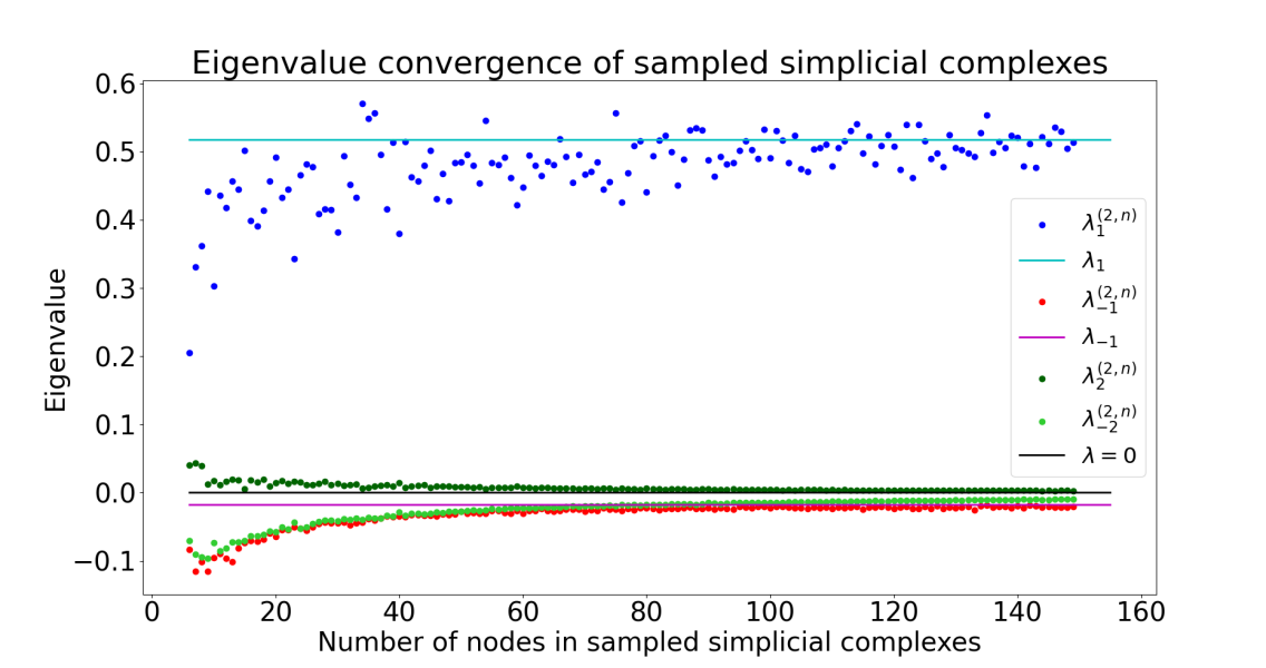
Fig. 1: Eigenvalue convergence of $\lambda_{i}^{(2,n)}$ for $i=1,2,-1,-2$.

6 Conclusion

In this work, we proposed a type of complexon shift operator based on marginal complexons, and find raised adjacency matrix as its corresponding shift operator for simplicial complexes. We proved that when a sequence of simplicial complexes converges to a complexon, then the eigenvalue sequences of raised adjacency also converge to the eigenvalue of the complexon shift operator. This conclusion is further supported by a numerical experiment on sampled simplicial complex sequences. The CSO and its eigenvalue convergence implies the transferability of SCSP on vertex signals, which suggests the potential application of complexon signal processing on large or dynamic simplicial complex networks.

References

• [1] T. Mitchell Roddenberry and Santiago Segarra, “Limits of dense simplicial complexes,” J. Machine Learning Research, vol. 24, no. 225, pp. 1–42, 2023.
• [2] Antonio Ortega, Pascal Frossard, Jelena Kovačević, José M. F. Moura, and Pierre Vandergheynst, “Graph signal processing: Overview, challenges, and applications,” Proceedings of the IEEE, vol. 106, no. 5, May 2018.
• [3] Aliaksei Sandryhaila and José M. F. Moura, “Discrete signal processing on graphs: Graph filters,” in Proc. IEEE Int. Conf. Acoustics, Speech, and Signal Processing, May 2013.
• [4] Luana Ruiz, Fernando Gama, Antonio García Marques, and Alejandro Ribeiro, “Invariance-preserving localized activation functions for graph neural networks,” IEEE Trans. Signal Process., vol. 68, pp. 127–141, 2020.
• [5] Franco Scarselli, Marco Gori, Ah Chung Tsoi, Markus Hagenbuchner, and Gabriele Monfardini, “The graph neural network model,” IEEE Trans. Neural Netw., vol. 20, no. 1, pp. 61–80, Jan 2009.
• [6] Fernando Gama, Antonio G. Marques, Geert Leus, and Alejandro Ribeiro, “Convolutional neural network architectures for signals supported on graphs,” IEEE Trans. Signal Process., vol. 67, no. 4, pp. 1034–1049, Feb 2019.
• [7] Xiaowen Dong, Dorina Thanou, Laura Toni, Michael Bronstein, and Pascal Frossard, “Graph signal processing for machine learning: A review and new perspectives,” IEEE Signal Process. Mag., vol. 37, no. 6, pp. 117–127, Nov 2020.
• [8] Wenlong Liao, Birgitte Bak-Jensen, Jayakrishnan Radhakrishna Pillai, Yuelong Wang, and Yusen Wang, “A review of graph neural networks and their applications in power systems,” Journal of Modern Power Systems and Clean Energy, vol. 10, no. 2, pp. 345–360, March 2022.
• [9] Santiago Segarra, Antonio G. Marques, and Alejandro Ribeiro, “Optimal graph-filter design and applications to distributed linear network operators,” IEEE Trans. Signal Process., vol. 65, no. 15, pp. 4117–4131, Aug 2017.
• [10] Songyang Zhang, Zhi Ding, and Shuguang Cui, “Introducing hypergraph signal processing: Theoretical foundation and practical applications,” IEEE Internet Things J., vol. 7, no. 1, pp. 639–660, Jan 2020.
• [11] Matthew W. Morency and Geert Leus, “Graphon filters: Graph signal processing in the limit,” IEEE Trans. Signal Process., vol. 69, pp. 1740–1754, 2021.
• [12] Jiying Zhang, Yuzhao Chen, Xi Xiao, Runiu Lu, and Shu-Tao Xia, “Learnable hypergraph laplacian for hypergraph learning,” in Proc. IEEE Int. Conf. Acoustics, Speech, and Signal Processing, May 2022, pp. 4503–4507.
• [13] Karelia Pena-Pena, Daniel L. Lau, and Gonzalo R. Arce, “t-HGSP: Hypergraph signal processing using t-product tensor decompositions,” IEEE Trans. Signal Inf. Process. Netw., vol. 9, pp. 329–345, 2023.
• [14] Zhiyang Wang, Luana Ruiz, and Alejandro Ribeiro, “Stability of neural networks on manifolds to relative perturbations,” in Proc. IEEE Int. Conf. Acoustics, Speech, and Signal Processing, May 2022, pp. 5473–5477.
• [15] Sergio Barbarossa and Stefania Sardellitti, “Topological signal processing over simplicial complexes,” IEEE Transactions on Signal Processing, vol. 68, pp. 2992–3007, 2020.
• [16] Feng Ji, Giacomo Kahn, and Wee Peng Tay, “Signal processing on simplicial complexes with vertex signals,” IEEE Access, vol. 10, pp. 41889–41901, 2022.
• [17] Luana Ruiz, Luiz F. O. Chamon, and Alejandro Ribeiro, “Graphon signal processing,” IEEE Trans. Signal Process., vol. 69, pp. 4961–4976, Aug. 2021.
• [18] Luana Ruiz, Luiz F. O. Chamon, and Alejandro Ribeiro, “The graphon Fourier transform,” in Proc. IEEE Int. Conf. Acoustics, Speech, and Signal Processing, Barcelona, Spain, 2020.
• [19] László Lovász, Large Networks and Graph Limits, American Mathematical Society, Providence, RI, USA, 2012.
• [20] C. Borgs, J.T. Chayes, L. Lovász, V.T. Sós, and K. Vesztergombi, “Convergent sequences of dense graphs I: Subgraph frequencies, metric properties and testing,” Advances in Mathematics, vol. 219, no. 6, pp. 1801–1851, 2008.
• [21] Edward B. Davies, Linear Operators and Their Spectra, Cambridge: Cambridge University Press, 2007.
• [22] Christian Borgs, Jennifer T. Chayes, László Miklós Lovász, Vera T. Sós, and Katalin Vesztergombi, “Convergent sequences of dense graphs II. multiway cuts and statistical physics,” Annals of Mathematics, vol. 176, pp. 151–219, 2012.
• [23] Jason Liang, “Measure-preserving dynamical systems and approximation techniques,” http://math.uchicago.edu/~may/REU2014/REUPapers/Liang,Jason.pdf, 2014.