Model-based traffic state estimation for link traffic using moving cameras

Abstract

Traffic State Estimation (TSE) is the process of inferring traffic conditions based on partially observed data using prior knowledge of traffic patterns. The type of input data used has a significant impact on the accuracy and methodology of TSE. Traditional TSE methods have relied on data from either stationary sensors like loop detectors or mobile sensors such as GPS-equipped floating cars. However, both approaches have their limitations. This paper proposes a method for estimating traffic states on a road link using vehicle trajectories obtained from cameras mounted on moving vehicles. It involves combining data from multiple moving cameras to construct time-space diagrams and using them to estimate parameters for the link’s fundamental diagram (FD) and densities in unobserved regions of space-time. The Cell Transmission Model (CTM) is utilized in conjunction with a Genetic Algorithm (GA) to optimize the FD parameters and boundary conditions necessary for accurate estimation. To evaluate the effectiveness of the proposed methodology, simulated traffic data generated by the SUMO traffic simulator was employed incorporating 140 different space-time diagrams with varying lane density and speed. The evaluation of the simulated data demonstrates the effectiveness of the proposed approach, as it achieves a low root mean square error (RMSE) value of 0.0079 veh/m and is comparable to other CTM-based methods. In conclusion, the proposed TSE method opens new avenues for the estimation of traffic state using an innovative data collection method that uses vehicle trajectories collected from on-board cameras.

1 Introduction

The term ”traffic state typically refers to the level of traffic, including its density, speed, and travel time, on a specific link on a road network. To effectively implement intelligent traffic management strategies and operations, it is crucial to accurately measure traffic conditions on the road network (links). These approaches are based on real-time data from large-scale road networks. However, it is not feasible to continuously monitor the entire network for extended periods of time, due to which traffic states in unobserved regions must be inferred using partially observed data. As a result, traffic state estimation has become a significant area of research in the field of transportation and has received considerable attention. Traffic State Estimation (TSE) involves inferring the flow, density, and speed of road segments based on partially observed traffic data and previous knowledge of traffic patterns (Seo . (2017)).

Recently, lightweight portable sensors such as smartphones, dashboard cameras (dashcams), and embedded devices have become popular and can be mounted on vehicles to capture traffic incidents. Due to their continuous interaction with the environment, such devices are a great source of urban data (Kumar . (2021)). In this article, we specifically refer to onboard vehicle-mounted cameras as moving cameras. With the advancement of in-vehicle camera technology, there is a huge potential for traffic detection using street-view video sequences, both at the macroscopic and microscopic levels. Using state-of-the-art computer vision algorithms and GPS measurements, the captured video sequence enables the extraction of vehicle trajectories, which can be used to generate space-time diagrams at the link level, as depicted in Fig.1. Compared to traditional stationary sensors such as loop detectors, the utilization of moving cameras allows for the collection of traffic state data with a higher spatial resolution along the entire link. Importantly, unlike the data obtained from floating car data (FCD), the proposed method does not require prior knowledge of the traffic penetration rate for analysis.

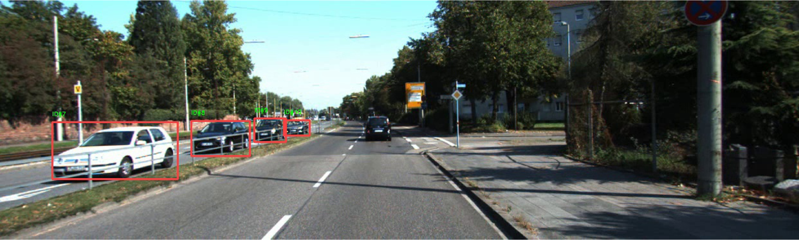
(a) Frame from a video sequence

(b) Space-time diagram from video

Figure 1: Example of space-time diagram generated from a video sequence captured by moving camera over a link. Original video is taken from Geiger . (2012).

By combining data from multiple vehicles with a camera moving along the link, it is possible to gather adequate space-time diagrams for estimating traffic states. However, certain areas within these diagrams may remain unobserved, as illustrated in Fig. 1 diagrams for estimating traffic states. The aim of this study is to develop and assess an innovative approach that leverages partially observed trajectories extracted from the space-time diagrams to estimate densities in the unobserved regions. This is achieved through a process of discretizing the space-time diagrams into small traffic density cells, followed by the application of the Cell Transmission Model (CTM) to estimate densities in the unobserved locations. To derive the Fundamental Diagram’s (FD) parameters and boundary conditions required for estimating traffic densities on the link, we employ a Genetic Algorithm (GA) to identify the optimal values for these parameters and conditions.

The remainder of the article is structured in the following manner: Section 2 provides a concise overview of the existing literature on the subject matter. The proposed TSE method is presented in Section 3. We first briefly present the computer vision algorithms that are used to infer the trajectories using a moving camera. Subsequently, the GA method, which estimates the FD parameters and densities in unobserved locations, is introduced. To evaluate the effectiveness of the proposed TSE method, various traffic scenarios generated using simulated data are tested. The experimental setup, results, and discussions on these tests are provided in Section 4. Finally, in Section 5, the article concludes by summarizing the analysis and suggesting potential avenues for future research.

2 Related Work

Ongoing research categorizes TSE into three fundamental components: input data, dynamic traffic flow models, and estimation methods. The input data in the TSE refers to the partial observations obtained from the road network, which serve as the basis for estimating the unobserved traffic states. Traffic flow models play a crucial role in describing the dynamics of traffic by incorporating physical principles and empirical relationships among various characteristics of the traffic flow. These models can be classified as macroscopic or microscopic. Macroscopic models focus on the aggregate behavior of traffic flow, while microscopic models consider the interaction between individual vehicles. Estimation methods encompass various approaches that aim to interpolate traffic states in unobserved regions using both traffic flow models and partial observations (Seo . (2017)).

TSE input data comes from a variety of sources, including loop detectors, radar sensors, GPS data, camera, radar, mobile phone data, etc. Stationary sensors, such as loop detectors, surveillance cameras, and radar-based sensors, typically provide traffic state measurements for a fixed location. Data from these sensors have been extensively used for estimation of travel time (Robinson  Polak (2005); Y. Li . (2018)), speed (Coifman  Kim (2009)), densities (Tampere  Immers (2007); Panda . (2019); Timotheou . (2015)), classification of jam conditions (Tyagi . (2012)) and various other traffic characteristics. Mobile sensors are usually vehicles with onboard sensors such as the Global Positioning System (GPS), onboard Diagnostics Systems (OBD), or embedded cameras that collect measurements along their trips. Such vehicles with fitted sensors are called probe vehicles or floating cars, and the data collected from them are called Floating Car Data (FCD). Multiple research studies have been conducted using FCD data to estimate traffic flow, speed, and density (Herrera  Bayen (2010); Sunderrajan . (2016); Yuan . (2021)).

Cameras have become a great source for urban traffic data collection systems. Early research in TSE used traffic data collected using fixed cameras, such as high-mounted surveillance or highway cameras. Pletzer . (2012); X. Li . (2013); Ua-Areemitr . (2019) used static cameras to estimate the mean speed, density, and level of service for a specific section of the road network visible by camera. Lately, there has been some research in which they focused on data collection with a moving camera and used it for TSE. Seo . (20151); Kumar . (2021) used the moving camera to collect data on the same lane or opposite lane for traffic analysis.

The traffic flow model typically describes a tangible model that portrays the dynamics of traffic, whereas the estimation methods comprise techniques used to determine the traffic condition based on limited observations and pre-existing knowledge of the traffic model. One of the most common models used in research is the first-order Lighthill-Whitham-Richards (LWR) model developed by Lighthill  Whitham (1955) and Richards (1956). Later, Daganzo (1994) proposed an explicit solution to the partial differential LWR system by discretizing the state space into homogeneous space-time cells, called the Cell Transmission Model (CTM). Several studies have utilized CTM in conjunction with various estimation methods to estimate traffic states. The TSE methodology was improved by Panda . (2019) by integrating a fundamental CTM to facilitate the propagation of traffic flow. The authors formulated filtering equations grounded on fundamental principles and utilized an enhanced Interactive Multiple Model (IMM) filtering methodology. The density estimation process was carried out using data obtained from loop detectors. The CTM model was utilized by Seo . (20152) to compute the density and parameters associated with the fundamental diagram. The researchers used the Ensemble Kalman Filter (EnKF) as an estimation technique, using data on the spacing of the heads. Timotheou . (2015) proposed a Moving Horizon Estimation (MHE) approach using asymmetric CTM for fault-tolerant TSE that achieves reliable estimation and simultaneously detects, isolates, and corrects measurements from periods of faulty sensor behavior. The density estimation process was executed by utilizing data acquired from loop detectors. Tampere  Immers (2007) presented a TSE model based on the CTM formulated in a closed analytical state-space form. This model was designed to be incorporated within a general Extended Kalman Filter (EKF) framework. Data collected from loop detectors was used for density estimation in their study.

Limited research is available that uses traffic data collected from cameras for TSE. Seo . (20151) utilized a Probe Vehicle Spacing Measurement Equipment (PVSME) that employed an onboard camera to capture the headway spacing between vehicles in the same lane as the probe vehicle. They later used these headway spacing data along with the Ensemble Kalman Filter (EnKF) as the estimation method for TSE (Seo . (20152)). Takenouchi . (2019) proposed a method based on Variational Theory (VT) to estimate traffic states. Their approach incorporated count measurements from a backward probe vehicle in the opposite lane, in addition to probe vehicle data in the same lane. The analysis focused on data collected during a single run on the network. Kumar . (2021) employed state-of-the-art computer vision algorithms to infer vehicle trajectories but did not provide a specific method for TSE.

In general, these previous studies that estimate traffic states based on traffic flow dynamics with various sensing data are valuable references for our study. However, none of them utilized measurements from a moving camera in the opposite lane for link-level TSE. Additionally, most TSE analyses assume or rely on pre-existing information or estimated boundary conditions for the link using various Kalman filter techniques. Therefore, the contributions of this study is to develop a model:

• for estimating traffic states on a link by utilizing data gathered from multiple moving cameras on the same link.

• capable of estimating states in the absence of boundary conditions for the link.

3 Framework

This study focuses on the link-level TSE, where the input data for the estimation method comprises multiple space-time diagrams generated using a moving camera. The moving camera utilizes advanced object detection and tracking algorithms to measure the trajectories of incoming vehicles, resulting in a space-time diagram of the link, as briefly discussed in Section 3.1. These diagrams are subsequently aggregated into density cells and employed to estimate densities in unobserved locations. The estimation process is explained in detail in Section 3.2, where we utilize observed cell densities to initially estimate parameters for the FD and later estimate the density in unobserved locations using the Genetic Algorithm GA that uses CTM as fitness function.

For TSE using the proposed methodology, the following information is assumed to be known. The position, length, and number of lanes of the link are considered pre-given information for the method. Additionally, multiple street view-video sequences are assumed to be recorded over the link, captured by the same vehicle at different times. The space-time cell dimensions used to discretize the space-time diagrams are selected prior to analysis. During the process of extracting vehicle trajectories from the street view video sequences, only vehicles that are visible in the video and traveling in the opposite lane are taken into account. This selection criterion ensures that distinct trajectories of all vehicles are obtained while traversing the link. Vehicles in the same lane are not considered, as they typically have speeds similar to those of the moving camera, which would not provide distinct samples. This approach aligns with the research conducted by Kumar . (2021); Takenouchi . (2019), which aimed to analyze traffic considering vehicles in the opposite lane.

3.1 Trajectory Extraction

The proposed method for TSE relies on space-time density diagrams representing vehicles’ trajectories extracted from street-view videos captured by an onboard camera mounted on a moving vehicle along a specific link in a road network. The research by Rastogi  Björkman (2023) present a trajectory extraction process consisting of three primary steps: multi-object detection, multi-object tracking, and estimation of lane distance. The initial step involves identifying and locating vehicles in the image, which is called Object Detection (OD). To achieve this, a Deep Neural Network (DNN) is employed to detect vehicles in each frame of the video sequence. Multiple frames are used to re-identify the same vehicle, assign a unique ID to it, and track it across subsequent frames, which is known as Multi-Object Tracking (MOT). Once vehicles are detected and labeled, their distance from the link on the road network is calculated using time-stamped GPS information, photogrammetry, and geodesy. This process, known as Lane Distance Estimation, calculates the distance for each detected vehicle. Finally, using distance and timestamp information, a space-time diagram is generated, where the spatial dimensions correspond to the link length and the time dimension represents the travel time of the camera-mounted vehicle. Fig.2 provides a visual representation of the complete process of extracting vehicle trajectories from a video sequence. In the illustration of the space-time diagram, the moving camera is depicted by a red dotted line, while the trajectories of detected vehicles are shown as lines with a red background.

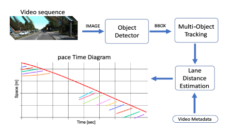
Figure 2: Flow chart to illustrates the process of extracting the vehicle trajectory from a street-view video sequence using different computer vision algorithms as presented in Rastogi  Björkman (2023).

3.2 Estimation Approach

The proposed TSE method, which utilizes space-time diagrams from a moving camera as input data, involves three key steps: discretization, FD calibration, and density estimation.

In the discretization process, we aggregate all the space-time diagrams into space-time cells with density information. Due to unobserved trajectories in certain regions, some cells do not contain any density information. To estimate the density of these unobserved cells, we employ the CTM method. The CTM method requires a calibrated FD of the link as well as boundary conditions on the link. The next two steps involve estimating optimal values for the FD parameters and the boundary conditions. In the FD calibration step, we utilize a GA-based method to find the optimal FD parameters by utilizing the cell densities in all observed cells. Following that, in the density estimation step, we utilize another GA-based method to find the optimal values for boundary conditions for each space-time diagram. Once we have the optimal values for both boundary conditions and FD parameters, we use them with CTM to estimate the density values for unobserved cells for each space-time diagram.

The CTM and GA implementation that is used in the proposed methodology is first described in the following part, and later each step in the estimation approach is expounded upon in the following sections after that.

3.2.1 CTM and GA

The proposed methodology is based on CTM according to which the density of cell $k$ in space $x$ and time $t+\Delta t$ depends only on the density values in $k(x,t)$; vehicle flow $Q(k(x,t),t)$ into the cell; vehicle flow $Q(k(x+\Delta x,t),t)$ out of the cell. The CTM can be expressed as:

$$k(x,t+\Delta t)=k(x,t)+\frac{\Delta t}{\Delta x}\left(Q(k(x,t),t)-Q(k(x+\Delta x,t),t)\right)$$ (1)

The flow $Q(k(x,t),t)$ in the above formulation is based on chosen link FD. Assuming a triangular flow-density relationship over the link, the $Q(k(x,t),t)$ is expressed as:

$$Q(k(x,t),t)=\min\left\{k(x-\Delta x,t)*v_{f}\;;w_{c}(k_{j}-k(x,t))\right\}$$ (2a)

$$w_{c}=\frac{v_{f}*k_{c}}{k_{j}-k_{c}}$$ (2b)

where $v_{f}$ is the free flow speed, $k_{c}$ is the optimal density, $k_{j}$ is the jam density and $w_{c}$ is the backward wave speed. The value of jam density $k_{j}$ can be calculated as the inverse of the minimum distance headway for all vehicles on the link.

The GA, created by John Holland John H. Holland (1992), is a computational optimization technique based on natural selection and evolution, initializing a population and iteratively evolving it through fitness calculation, selection, crossover, and mutation until the best solution is found or the maximum number of generations is reached. In our proposed methodology, we have customized the original GA to determine the optimal parameters for FD and boundary conditions. The flow chart illustrating the utilization of the GA in our methodology is presented in Fig. 3.

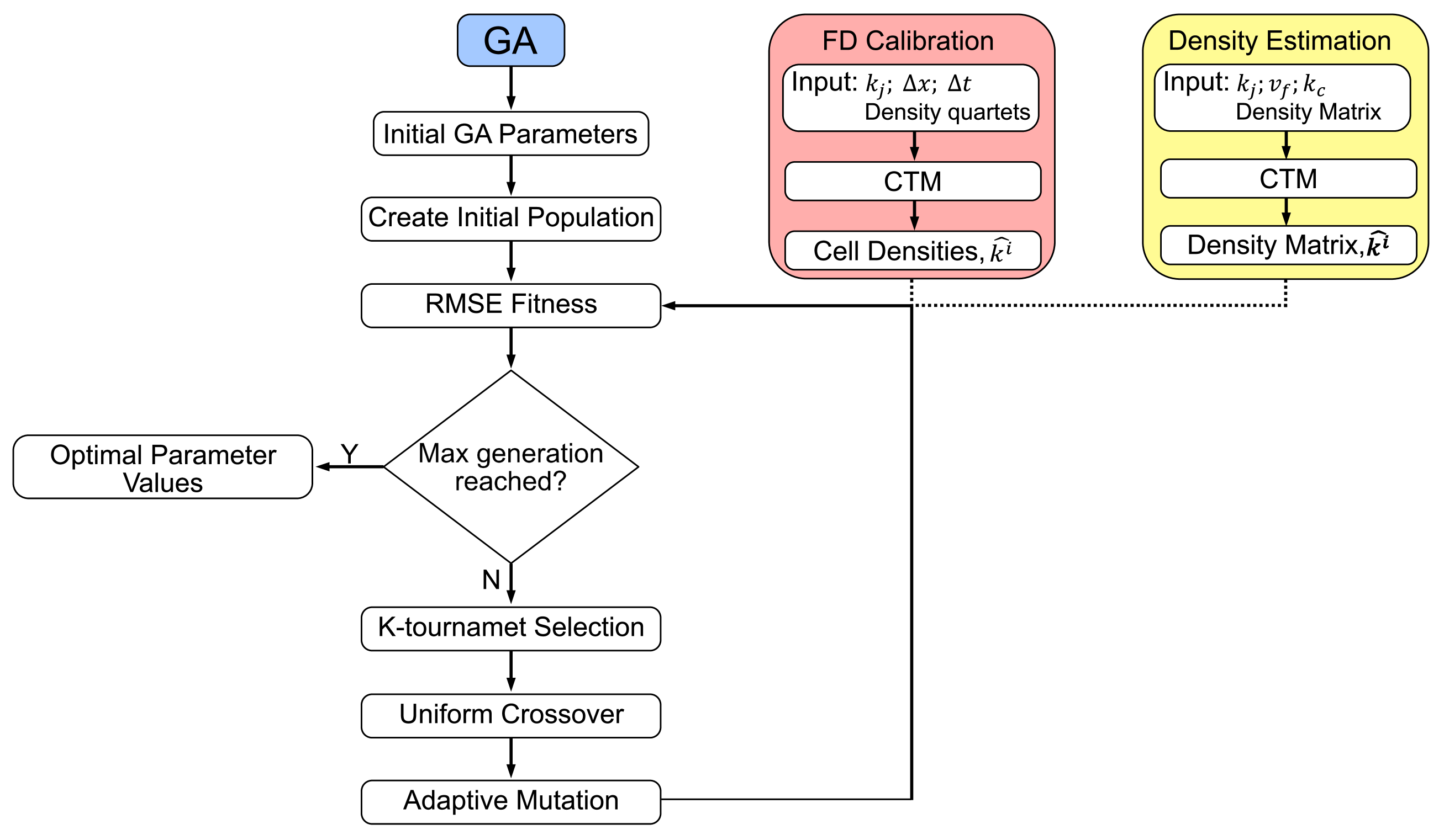
Figure 3: Flow chart of the proposed GA method for FD calibration and density estimation using CTM for fitness evaluation..

The GA algorithm commences by generating a set of candidate solutions that are randomly initialized. These candidates represent potential values for either the FD parameters or boundary conditions, serving as potential solutions to the optimization problem.

Subsequently, the fitness of each candidate is evaluated using a fitness function, which measures an individual’s fitness or competitive ability compared to others. In our methodology, we incorporate the CTM as part of the fitness evaluation. The specific fitness calculations for FD parameter calibration and density estimation are explained in Section 3.2.3 and Section 3.2.4, respectively.

The next step involves selecting the fittest individual to pass their genetic information to the next generation. We employ the K-way tournament selection procedure, as described by Katoch . (2021). This procedure randomly selects K candidate solutions from the population and chooses the one with the highest fitness as the parent for the subsequent steps of the GA. This selection process is repeated until the desired number of parents in the mating pool is attained.

The selected candidate solutions from the K-way tournament selection are then combined to create a new population for the next generation. We adopt a uniform crossover algorithm, as described in Katoch . (2021)), as it preserves the structural form of the candidate solutions. Unlike other standard crossover algorithms, the uniform crossover treats each gene independently instead of segmenting the solution.

Before proceeding to the next iteration, some of the candidate solutions undergo mutation. We employ an adaptive mutation method described by Marsili Libelli  Alba (2000). This method defines two distinct mutation probabilities based on the fitness value of each candidate. Solutions with a fitness value below a threshold undergo a higher mutation rate, while those with higher fitness values experience a lower mutation rate. The mutation is applied to each candidate solution based on its fitness value.

3.2.2 Discretization

The first step of the estimation process is to define and aggregate the measured space-time trajectory into a space-time density matrix. Each space-time diagram of the total time $T$ and the total length of the link $L$ is divided into discrete space-time cells. The dimensions of each cell are given by the size of the cell $\Delta x$ and the length of the time step $\Delta t$. Therefore, each space-time matrix will have dimension $(\alpha\times\beta)$, where $\alpha$ is the total number of space cells and $\beta$ is the total number of time cells. The value of $\alpha$ and $\beta$ is given by:

$$\alpha=\frac{L}{\Delta x}$$ (3a)

$$\beta=\frac{T}{\Delta t}$$ (3b)

The density $k(x,t)$ of cell $x$ during time $t$ is calculated using Edie (1963) generalized definitions of traffic states in a given space-time region. According to Edie, the density $k(\mathbf{A})$ in a space-time region $\left|\mathbf{A}\right|=\Delta x*\Delta t$ is derived as:

$$k(\mathbf{A})=\frac{\sum_{j}t_{j}(\mathbf{A})}{\left|\mathbf{A}\right|}$$ (4)

where $t_{j}(\mathbf{A})$ is the total time spent by the unique vehicle $j^{th}$ within $\left|\mathbf{A}\right|$.

Fig. 4 illustrates the aggregation of a space-time trajectory diagram into a space-time density matrix. The cells in the matrix contain density information, indicating the observed traffic states obtained from the visible vehicle trajectories captured in the video. This discretization process is performed for all video sequences recorded on the link, resulting in multiple space-time density matrices representing the link. These partially observed density matrices serve as the input for the estimation method proposed in this study.

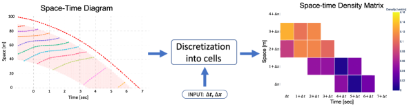
Figure 4: Example of discretization of space-time trajectories to the space-time density matrix. The empty spaces in the density matrix correspond to unobserved states.

3.2.3 FD Calibration

To estimate the optimal parameter values for triangular FD, we utilized the cell densities from all discretized space-time diagrams from previous step. According to the CTM formulation in Eq.1 and Eq.2, the cell density $k(x,t+\Delta t)$ only depends on the value of $k(x,t)$; $k(x-\Delta x,t)$; $k(x+\Delta x,t)$ and FD parameters - $v_{f}$, $k_{c}$ and$k_{j}$. Given the other values in CTM formation, we can find the values of $v_{f}$ and $k_{c}$ that best satisfy the relation.

For this purpose, we extract the cell densities in the following exact formation, called quartets - $k(x,t)$; $k(x-\Delta x,t)$; $k(x+\Delta x,t)$ and $k(x,t+\Delta t)$, from all space-time density matrices. Fig. 5 shows an example of a space-time density matrix where the cells marked with a ”green” boundary are the cell densities of the given matrix used for the FD estimation.

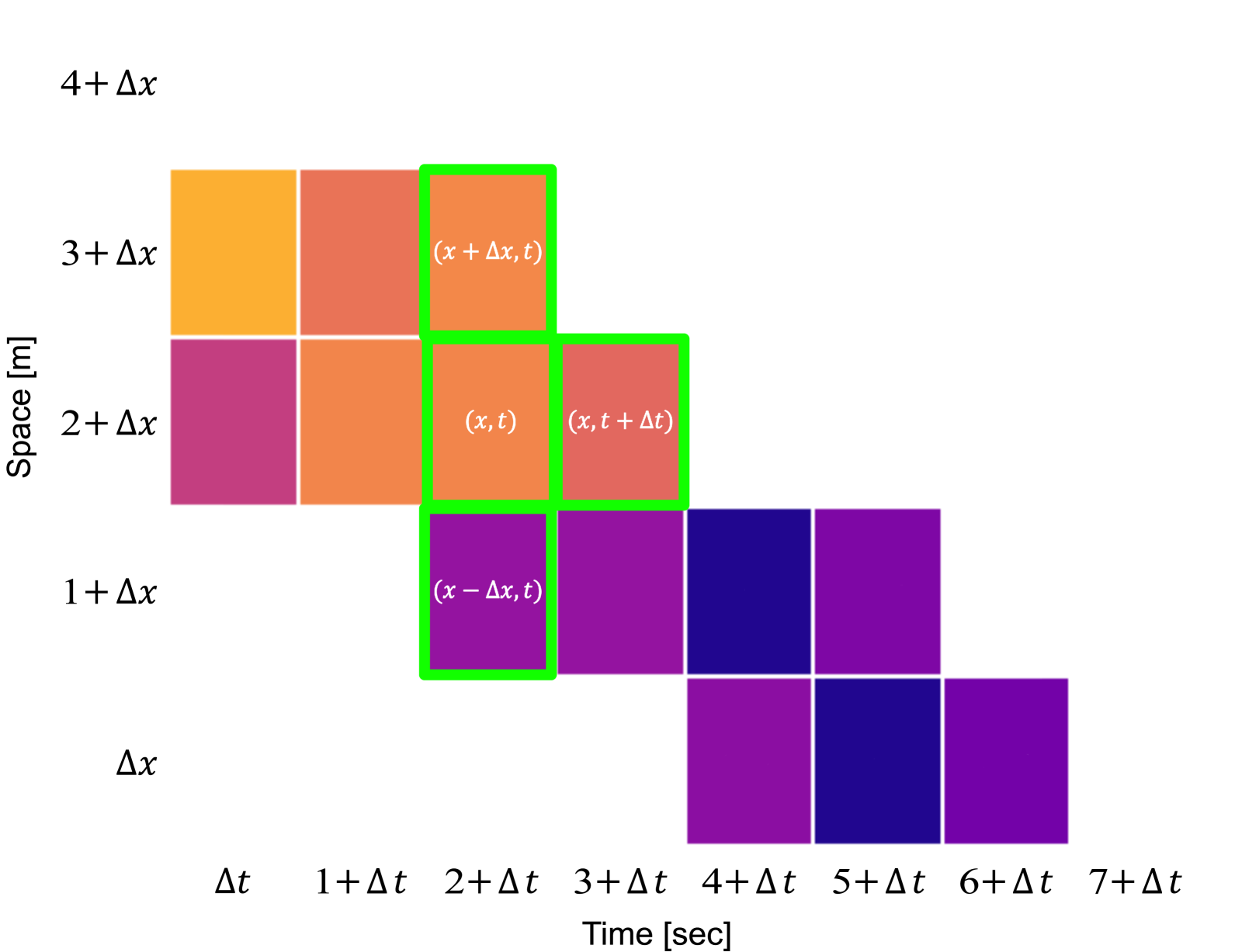
Figure 5: Example of a space-time matrix where cells with a ”green” boundary re-present a quartets that is used to calibrate the triangular FD.

The GA method, as described in Section 3.2.1, is utilized to determine the optimal values of $v_{f}$ and $k_{c}$ that satisfy Eq.1 for all quartets of cell densities.

To initialize the GA, the population is generated by pairing sampled values of $v_{f}$ and $k_{c}$ from a uniform distribution, considering certain constraints. The value of $v_{f}$ is limited by the Courant-Friedrichs-Lewy (CFL) condition, which states:

$$v_{f}\leq\frac{\Delta x}{\Delta t}$$ (5)

Similarly, the value of $k_{c}$ is constrained to always be less than half the jam density $k_{j}$. This constraint arises from the observation that congestion propagates through the mainstream at a slower speed than the maximum traffic speed. Therefore, the value of $k_{c}$ is given as:

$$w_{c}<v_{f}\Rightarrow\frac{k_{c}}{k_{j}-k_{c}}<1\Rightarrow k_{c}<\frac{k_{j}}{2}$$ (6)

We utilized Root Mean Square Error (RMSE) for FD calibration step, to determine the fitness of each possible solution in GA process. The fitness of the $i^{th}$ pair of $v_{f}$ and $k_{c}$ in GA is calculated as RMSE value between the actual density $k(x,t+\Delta t)$ and calculated density $\widehat{k}$ using Eq.1. The value of fitness for $N$ density quartets is expressed as:

$$RMSE=-\sqrt{\frac{1}{N}\sum_{i=0}^{N}\left(k^{i}(x,t+\Delta t)-\widehat{k^{i}}\right)^{2}}$$ (7)

3.2.4 Density Estimation

To propagate traffic states on a link using the CTM, boundary condition values are required. These include initial cell densities ($k(x,t=0)\forall x$), inflow into the link ($Q(x=0,t)\forall t$), and outflow from the link ($Q(x=\alpha,t)\forall t$). With these values and the link’s FD, the traffic states on the link at each timestep can be estimated by propagating the initial cell densities.

In this step of the proposed methodology, we estimate the boundary conditions for each space-time density matrix using the GA method descirbed in Section 3.2.1. The goal is to find a combination of boundary conditions that can accurately estimate the observed cell densities using CTM.

In this particular GA, each possible solution is represented as a vector consisting of initial cell densities, inflow, and outflow. The elements in the vector are sampled from a uniform distribution between 0 and $k_{j}$. The inflow and outflow values are also sampled as densities, and the flows are calculated using a triangular FD function $Q(k(x,t),t)$ during the CTM. Fig.6 illustrates the arrangement of the solution vector used in the GA.

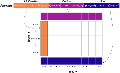
Figure 6: Illustration showing an arrangement of vector solution used to simulate CTM in the GA estimation algorithm.

To calculate the fitness of each solution, we execute the CTM with the calibrated FD parameters and boundary conditions to generate a density matrix $\mathbf{\widehat{k}^{i}}$ of dimension $(\alpha\times\beta)$. This resultant density matrix is then compared with the actual density matrix $\mathbf{k}$ with observed density cells. The fitness value for the solution is determined as the negative root mean square error (RMSE) calculated between the actual and CTM-calculated matrices.The value of fitness for $i^{th}$ solution is expressed as:

$$RMSE=-\sqrt{\frac{1}{(\alpha\beta)}\sum_{x=0}^{\alpha}\sum_{t=0}^{\beta}(\mathbf{k}-\mathbf{\widehat{k}^{i}})}$$ (8)

4 Testing on Simulated Data

To establish the reliability and precision of the proposed TSE method in various traffic scenarios, experiments were carried out using simulation-generated data. Given the practical challenges associated with collecting real-world data for all possible traffic conditions, simulation-based data provide a more feasible alternative for comprehensive analysis. By controlling the simulation parameters, various traffic scenarios can be generated for both incoming and parallel lane traffic.

4.1 Setup

To test the proposed TSE method, we use data generated with the Simulation of Urban Mobility (SUMO). SUMO is an open-source microscopic simulation of road traffic. Traffic simulations are generated using a microscopic, space-continuous, and time-discrete car-following model and a lane-changing model. As highlighted in Lopez . (2018), SUMO is a popular tool to generate simulated traffic and is highly respected in the research community.

Fig. 7 illustrates the bidirectional road configuration employed in SUMO to generate the data. This particular network consists of a single lane in each traffic direction, spanning a length of $100$ meters and featuring two traffic lights for division. Within this network, an aqua-colored car acts as moving camera. The shaded red box positioned ahead of this vehicle represents the simulated field of camera view, mirroring the real-world camera’s range under which vehicles can be detected through image processing techniques. In a real-world situation, the onboard camera usually has a limited range of vehicle detection. Therefore, we assume that vehicles between $10$ and $60$ meters from the moving camera vehicle are visible and will be considered for analysis. For simulation purposes, the traffic on the link is generated randomly and subjected to the following parameter values as given in Table. 4.1

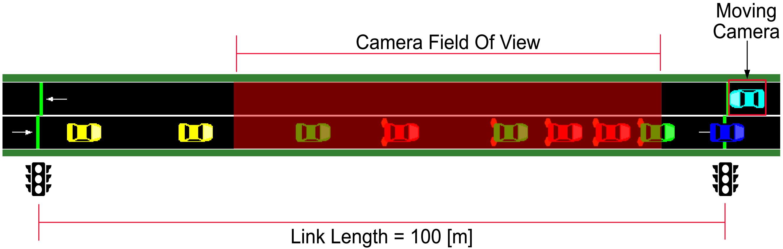
Figure 7: Bidirectional road in SUMO to generate simulation data. The probe vehicle simulates the moving camera. The red-shaded region in front of the probe vehicle represents the camera field of view.

Parameters for SUMO generated data. Parameters Explanation Value $v_{f}$ free flow speed $10$ m/s $s_{min}$ minimum headway distance $6.5$ m $fov$ camera field of view $\left[10,60\right]$ m $L$ total link length $100$ m $\Delta x$ space cell dimension $20$ m $\Delta t$ time cell dimension $2$ s

A total of 140 unique traffic space-time diagrams were generated, each consisting of a single continuous run of a moving camera on the road network. The number of vehicles generated in each lane of the network was varied to create traffic scenarios with different density and speed conditions. The 140 scenarios combined have the a free-flow speed $v_{f}$ of $8.55m/s$ and an optimal density $k_{c}$ of $0.0577veh/m$ with a triangular FD as shown in Fig.8. The speed and the density on the link are equally distributed across all the scenarios and is presented in Fig.9a and Fig.9b, respectively.

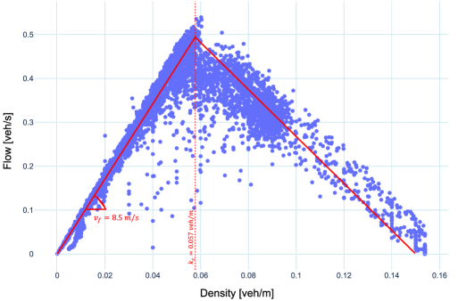
Figure 8: Flow-density curve of the simulated road for 140 scenarios generated using SUMO. The FD has a free-flow speed of $8.55m/s$ and optimal density of $0.0577veh/m$.

(a) Speed distribution of traffic.

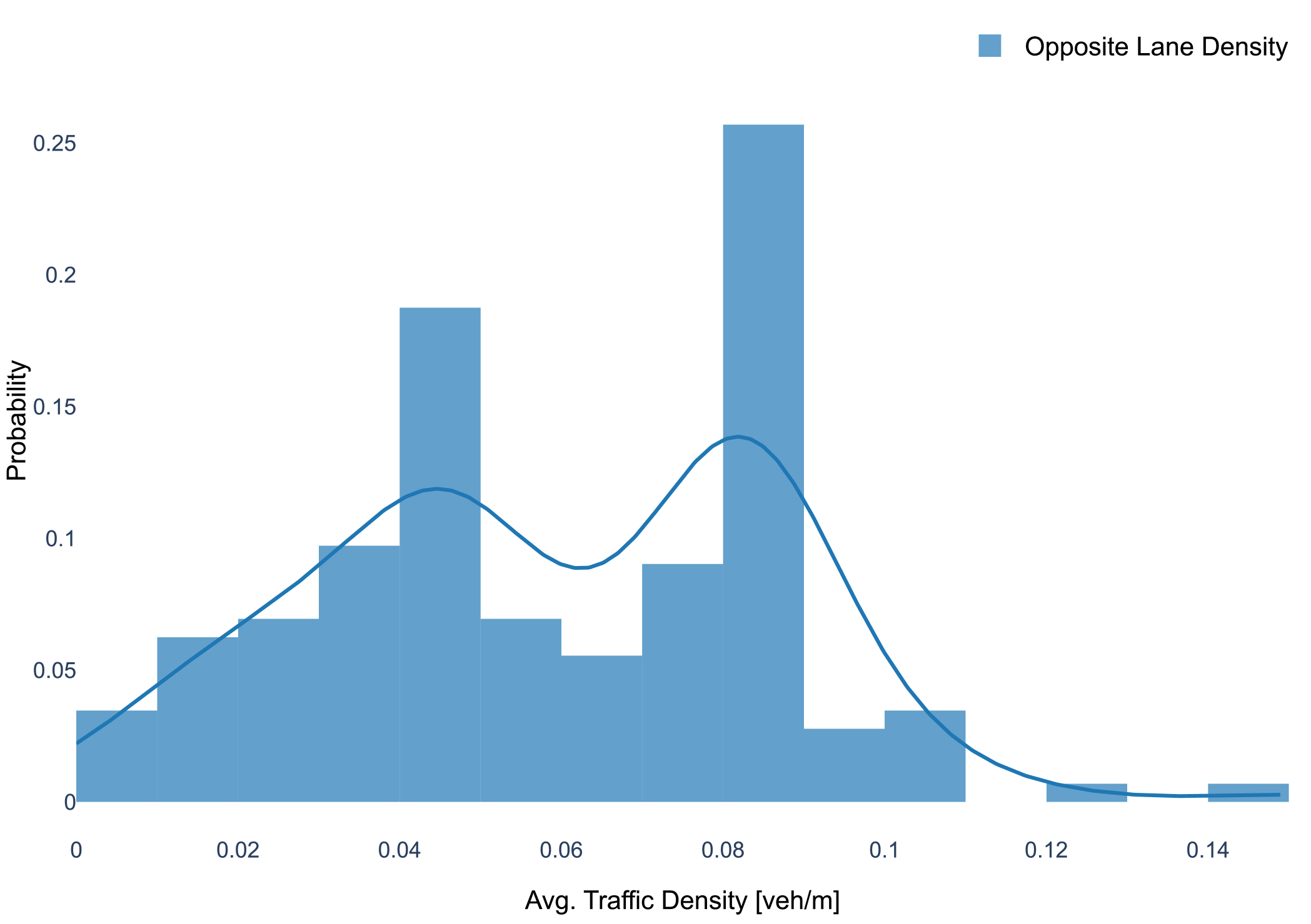
(b) Density distribution of traffic.

Figure 9: Distribution of the speed and density of the simulated data on the link in all 140 space-time diagrams. The speed distribution plot shows the spread of the average speed of the camera moving on the link and the average speed of traffic on the opposite lane.

In Fig.10, we showcase an example of a simulated space-time diagram generated by SUMO. The trajectories produced by SUMO are displayed in the top left plot, where the red dashed line represents the path followed by the moving camera, while the other lines depict the trajectories of vehicles in the opposing lane. This plot serves as a representation of the ground truth data for the link. Furthermore, the trajectories presented in the top-right plot illustrate the paths that are captured by the moving camera as it traverses the link. The trajectories within the red-shaded region in the plot correspond to the moving camera’s field of view, while the partial trajectories represent the measured data that will be utilized in the proposed TSE methodology. All the space-time diagrams undergo the discretization step described in Section 3.2.2, using the given value of the space cell $\Delta x$ as $2$ m and the length of the time step $\Delta t$ as $20$ sec. The bottom two plots present an example of the resultant space-time matrix of dimension $(\alpha\times\beta)=(5\times 8)$ after the discritization step on the space-time diagram..

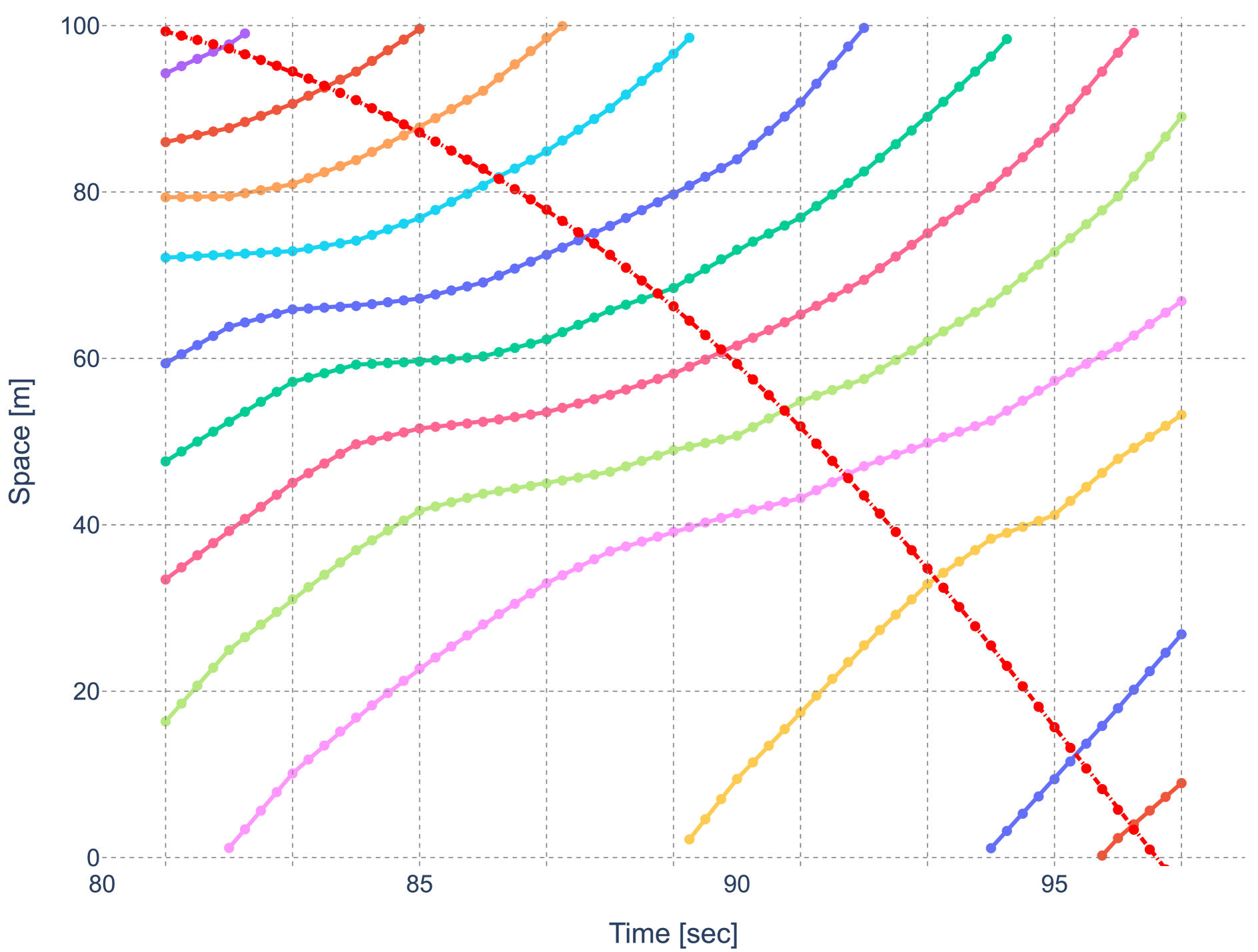
(a) Ground truth trajectories

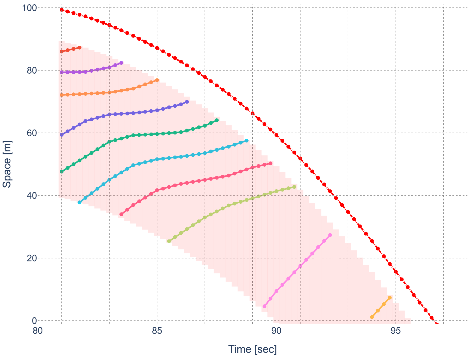
(b) Camera measured trajectories

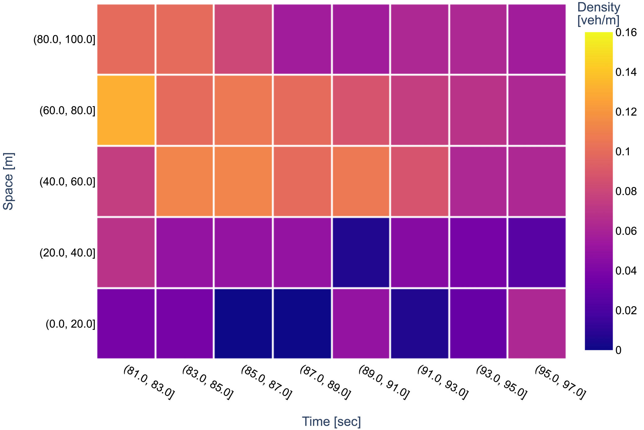
(c) Ground truth matrix

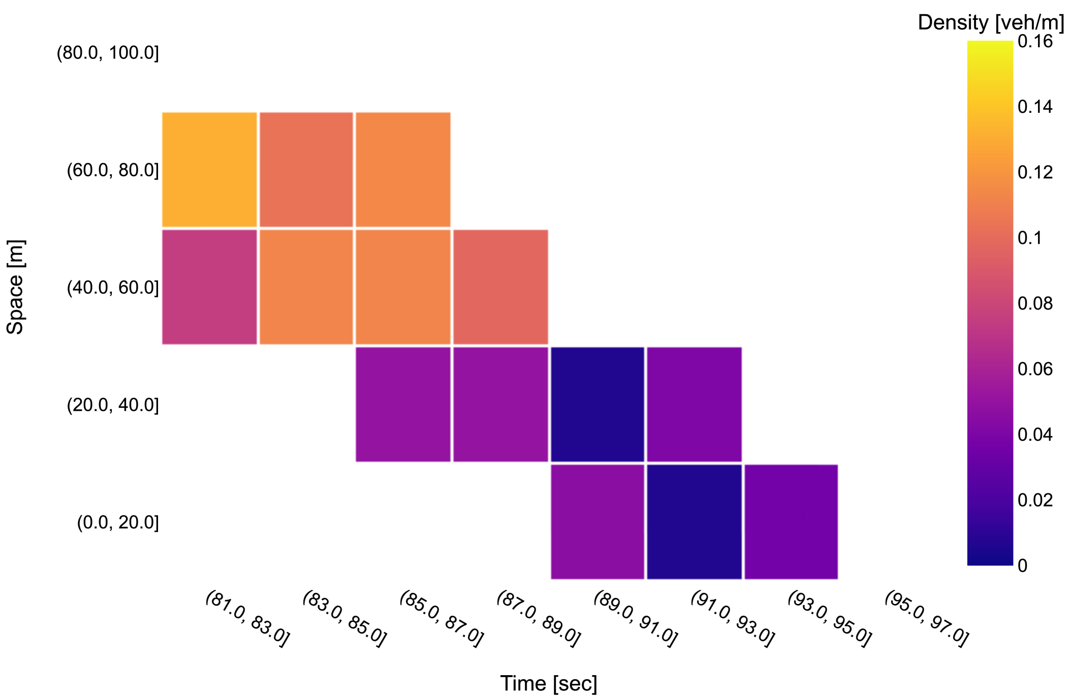
(d) Partial matrix

Figure 10: Example of a traffic space-time diagram generated using SUMO showcasing the actual trajectories as well as the respective aggregated space-time density matrices.

4.2 Analysis of CTM with known values

Since the proposed methodology relies on utilizing the CTM to estimate missing density values within space-time matrices, our initial analysis focuses on assessing the effectiveness of CTM in estimating values based on known values for calibrated FD relationships and boundary conditions. To accomplish this, we employed the known FD parameter and boundary values obtained from the 140 space-time diagrams. Subsequently, we conducted CTM simulations for each of these scenarios and compared the resulting space-time matrices with the corresponding ground truth matrices.

For result comparison purposes, we adopted the Root Mean Square Error (RMSE) as the evaluation metric. RMSE is a widely utilized measure in the research community and has been employed by other researchers like Van Erp . (2017); Seo . (20152). In our analysis, we specifically focused on considering cells located below the trajectory of the moving camera. This selection was made due to the absence of information regarding the outflow in the opposite lane. Consequently, predicting traffic flow beyond the passage of vehicles in the opposing lane becomes unfeasible, necessitating the exclusion of such cells from our analysis. Fig. 11 shows the cells located below the moving camera trajectory that are considered for the RMSE calculation.

(a) Ground truth matrix

(b) CTM Result

Figure 11: CTM analysis for example in Fig. 10 highlighting only the cells that are considered in actual output and the result obtained from CTM for RMSE calculation.

Fig. 12 illustrates the distribution of RMSE values between the actual output and the results obtained from CTM simulations using known FD parameters and boundary conditions. Across the 140 space-time diagrams examined, the average RMSE was found to be 0.0058 veh/m, with a standard deviation of 0.0032.

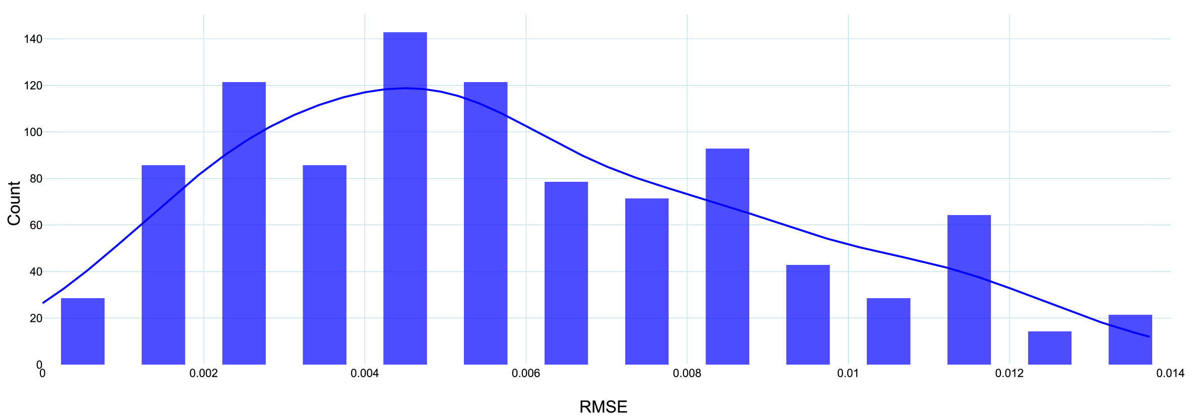
Figure 12: Distribution of RMSE between ground truth matrix and CTM output from the known values of FD and boundary conditions.

From the above analysis, we can conclude that even with the incorporation of known boundary conditions and FD values, a notable discrepancy persists between the actual output and the output derived from CTM. This disparity in precision can be attributed to the inherent limitations of discretization. When aggregating space-time diagrams into density cells, we make the assumption of homogeneity within each cell, thereby eliminating transient changes occurring within the cell. CTM heavily relies on this assumption. The disparity between the cell values generated by CTM and the actual data may stem from CTM’s inability to accurately replicate transient states. This analysis aligns with previous research conducted by Munoz . (2004); Sumalee . (2011), who similarly identified this limitation of CTM and proposed extensions to address and mitigate it.

4.3 Analysis of proposed TSE

The subsequent focus of our study is on the ability of the proposed TSE method to generate FD parameters and boundary conditions for each space-time diagram using only the partial matrices as input data. We will present the analysis and results from the FD calibration step and followed by the application of the calibrated FD in the density estimation step to estimate unobserved density cells, in the following sections.

4.3.1 FD parameter estimation

The FD calibration step uses the density quartets, which are explained in detail in Section 3.2.3, as input for the proposed GA. From the 140 partial density matrices, we were able to extract approximately 194 quartets. We generated the $56$ paired sample of $v_{f}$ and $k_{c}$ from a uniform distribution, subject to constraints given by Eq.5 and Eq.6. Through repeated experiments, we determined the optimal parameters for the GA as follows: generations = $100$, k-tournament = $5$, adaptive mutation probabilities = $(0.65,0.35)$ and crossover fraction = $20$. The experimental procedure and the results to obtain the best GA parameters for the FD calibration are presented in Appendix A. As the GA does not guarantee a global optimal solution, we ran the GA procedure five times with the same parameters to ensure consistent results. The best output from these runs was selected as the final result.

The GA estimated optimal values for $v_{f}$ and $k_{c}$ are $8.586$ m/s and $0.0525$ veh/m, respectively, with a RMSE value of $0.015$ veh/m. These estimated values closely align with the actual FD parameter values of $v_{f}$ = 8.55 m/s and $k_{c}$ = 0.057 veh/m. In Fig. 13a, we present the triangular FD derived from the estimated parameter values obtained by the GA, demonstrating its close proximity to the actual FD. Moreover, employing the optimal values obtained from the GA, the CTM formulation outlined in Eq. 1 exhibits minimal error in predicting the density values at $k(x,t+\Delta t)$, as illustrated by the residual plot in Fig. 13b.

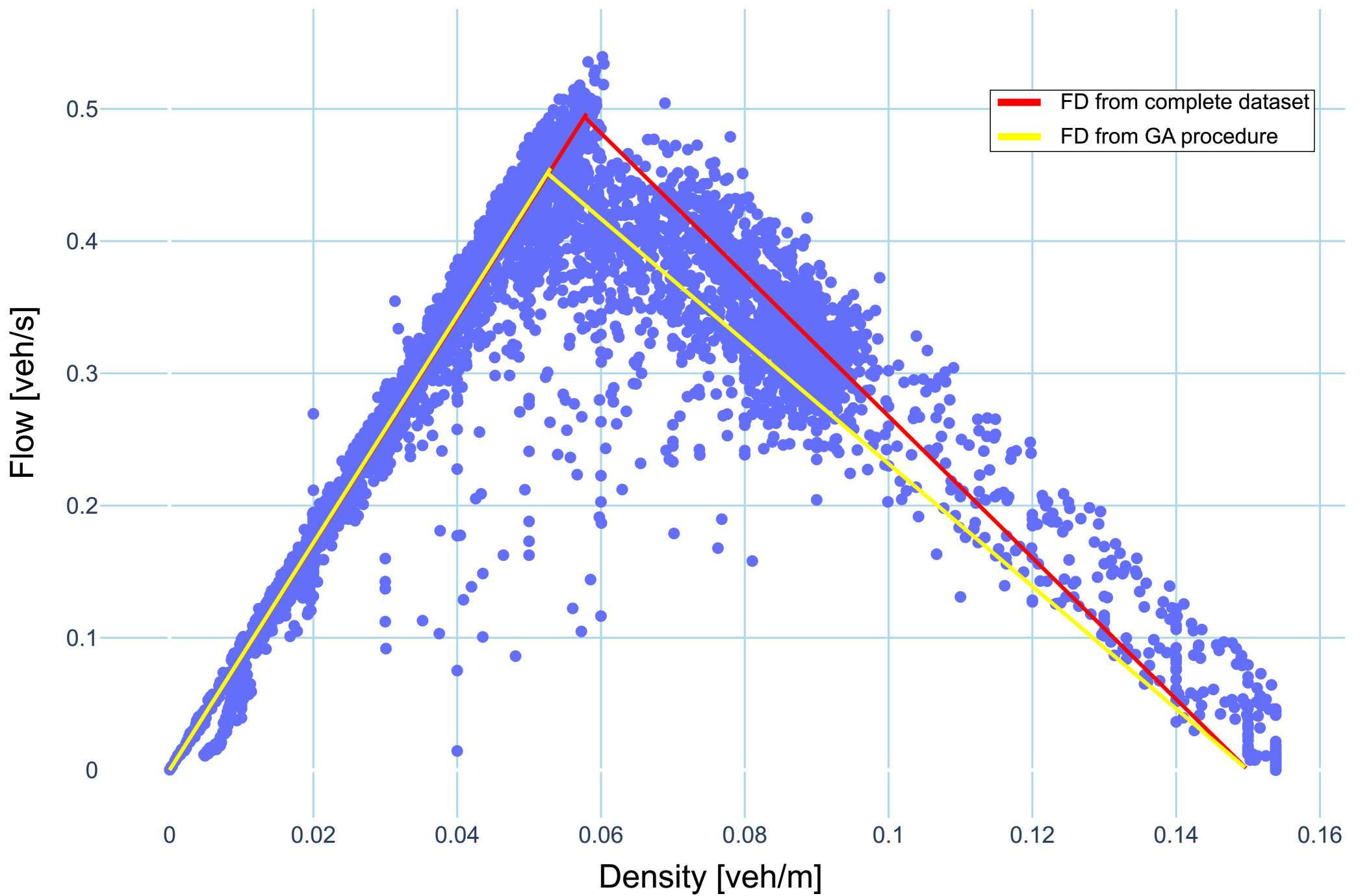
(a) Flow-density curve

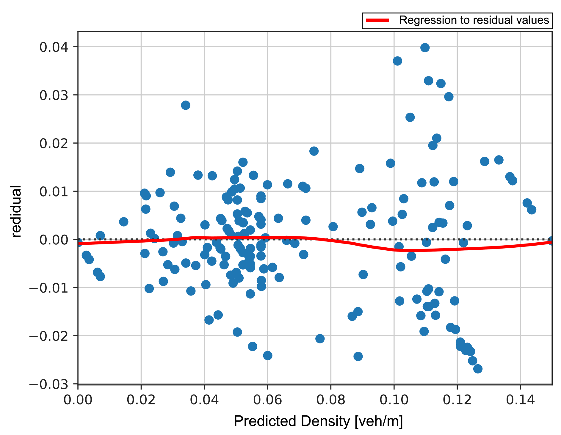
(b) Residual plot

Figure 13: Result of the FD calibration step using GA method. The left figure shows the difference in the actual FD (red) and the estimated FD (yellow). The right figure shows the error residual plot between the actual cell densities and estimated cell densities. The red curve is the regression to the residuals.

Based on the analysis, we can conclude that the proposed GA method is capable of calibrating triangular FD parameters with a limited number of density quartets, although a small error is observed. The discrepancy in the calibration of FD parameters could be attributed to the limited amount of data utilized in the GA calibration process. To improve the accuracy of parameter estimation, it is crucial to incorporate a diverse range of quartets values that cover the entire flow-density range. Also, increasing the amount of data can help mitigate errors during the estimation process.

4.3.2 Density estimation

The subsequent step in the proposed methodology involves estimating the boundary conditions for all 140 space-time matrices, with the aim of accurately estimating the observed density cells using the CTM in conjunction with the calibrated FD parameters and estimated boundary conditions.

To initiate the GA process, an initial population is generated, where each solution represents a vector combination of boundary conditions, as described in Section 3.2.4. The vector values are randomly selected from a uniform distribution within the range of $[0,k_{j}]$. Through multiple experiments, we determined the optimal parameters for the GA as follows: generations = 60, population size = 500, k-Tournament = 10, adaptive mutation probabilities = (0.9, 0.1), and crossover fraction = 50. A detailed account of the experimental procedure and the results to obtained from the best GA parameters for the boundary condition estimation is provided in Appendix B. Similar to the FD calibration step, since the GA does not guarantee a globally optimal solution, we conducted five runs of the GA procedure with the same parameters to ensure consistent outcomes. The best output from these runs was selected as the final result.

Once the optimal boundary conditions are obtained from the GA, they are combined with the calibrated FD values to generate the density cell values for the entire space-time domain, representing the final outcome of the proposed methodology. This process is repeated for each of the 140 space-time matrices in the experiment, resulting in a total of 140 runs of the GA method.

Similar to the analysis in Section 4.2, we calculate the RMSE between the ground truth and the output of GA after the procedure for each scenario, specifically focusing on the cells located below the trajectory on the moving camera. The Fig. 14 shows the cells located below the moving camera trajectory that are considered for the RMSE calculation.

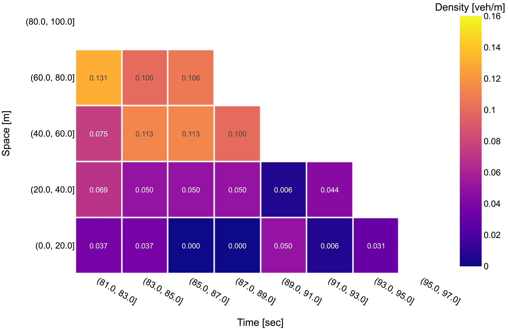
(a) Ground truth matrix

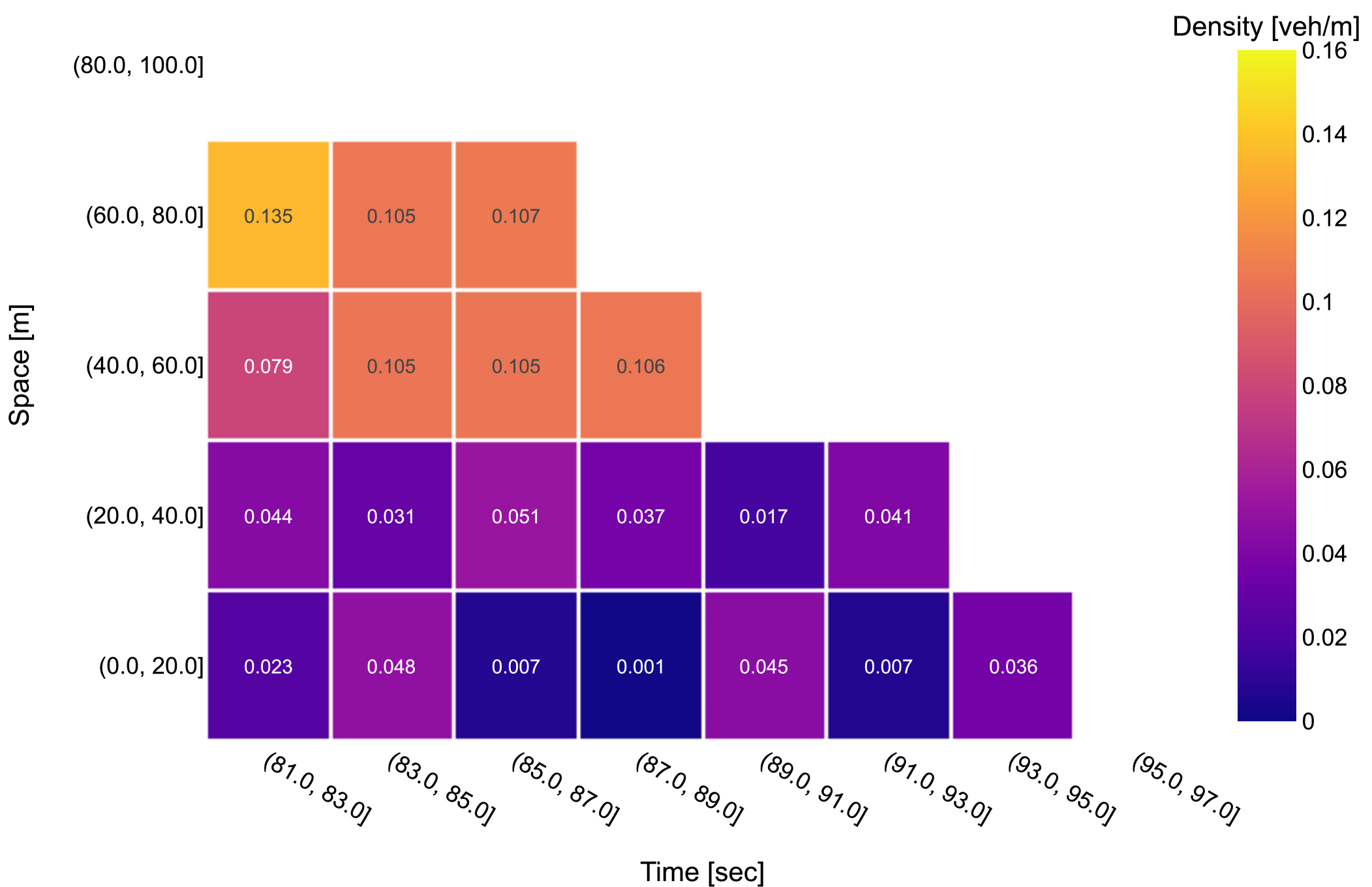
(b) GA Result

Figure 14: Result of GA for example presented in Fig. 10. The plot highlights the cells that are considered in actual output and the result obtained from GA for RMSE calculation.

Figure 12 presents the distribution of RMSE values between the actual output and the results obtained using the estimated FD parameters and boundary conditions derived from the GA procedure. When analyzing the 140 space-time diagrams, the average RMSE was determined to be 0.0079 veh/m, with a standard deviation of 0.0043. Additionally, the figure includes the RMSE values between the actual output and the results obtained from CTM simulations using the known FD parameters and boundary conditions, serving as a basis for comparison.

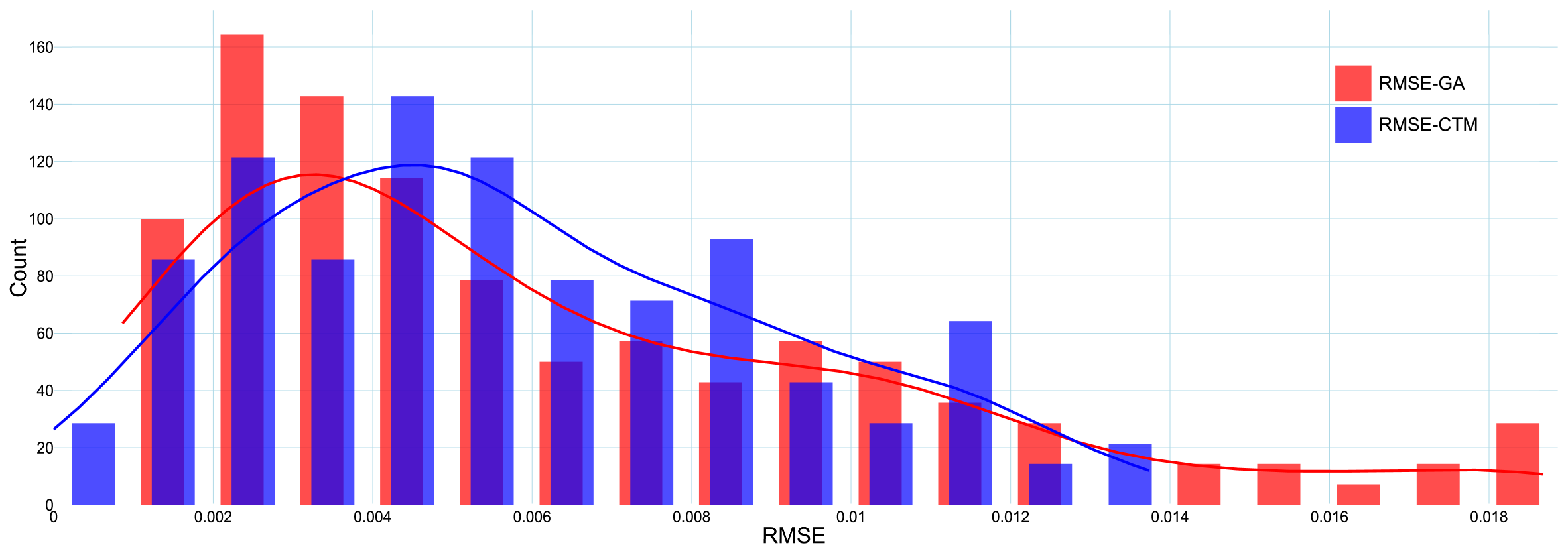
Figure 15: Distribution of RMSE between ground truth matrix and GA output as well as CTM output from the known values of FD and boundary conditions.

We also investigated the influence of different traffic states on the output of the proposed TSE method by analyzing the resulting RMSE in relation to the speed and density of traffic on the link in all scenarios. To explore this relationship, we utilized the Huber Regressor, a robust L2-regularized linear regression model designed to handle outliers. Fig.16 shows the RMSE values corresponding to the variable density of traffic in the opposite lane and the moving camera speed over the link. The regression analysis reveals that both the RMSE values obtained from the GA and CTM exhibit a positive trend with increasing link density, with respective correlation coefficients of $0.3127$ and $0.206$. In contrast, the RMSE values do not exhibit a significant dependence on changes in the moving camera speed. The regression analysis indicates a small correlation coefficient of $0.001$ for the RMSE with GA and $0.016$ for the RMSE with the CTM output.

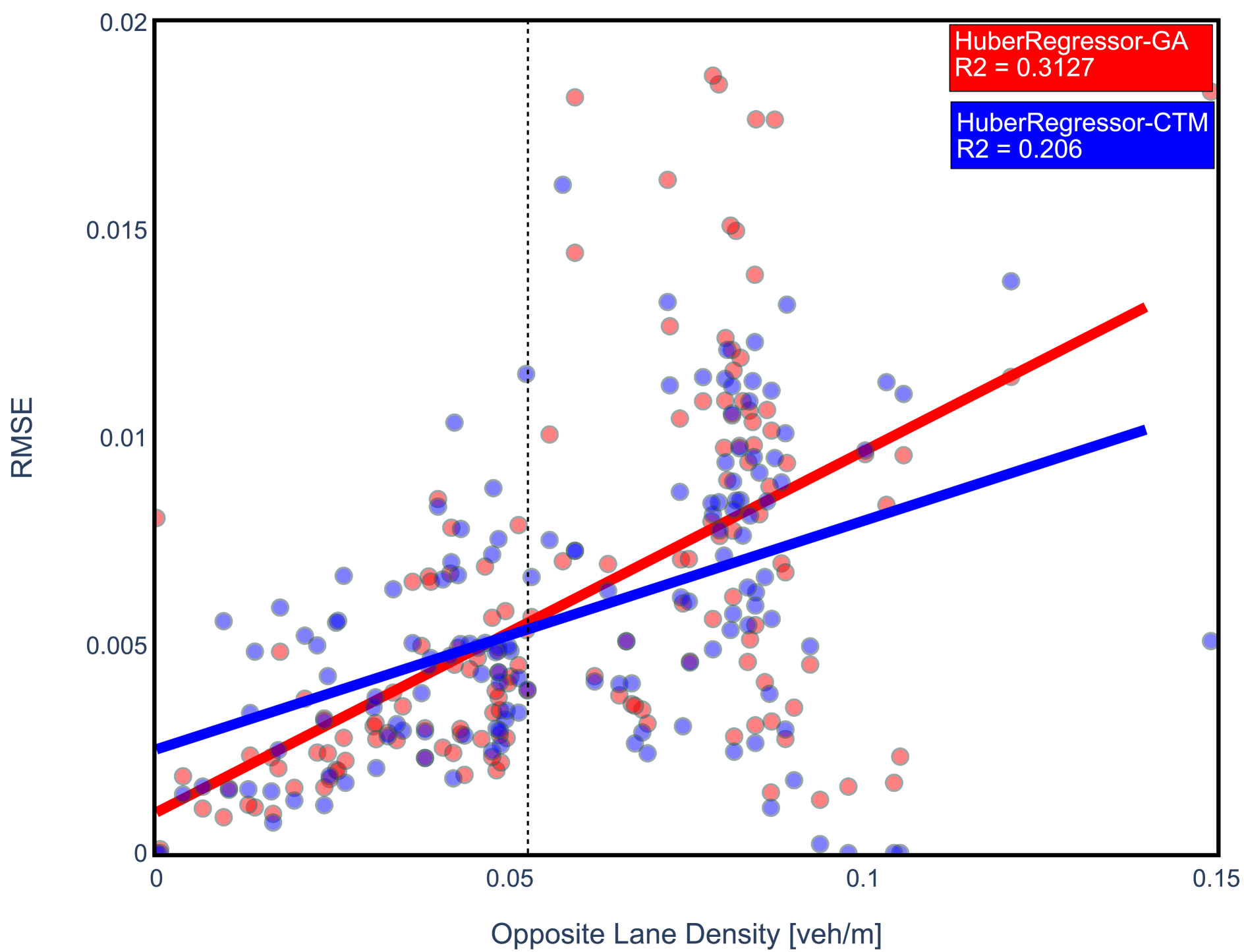
(a) RMSE vs Link density

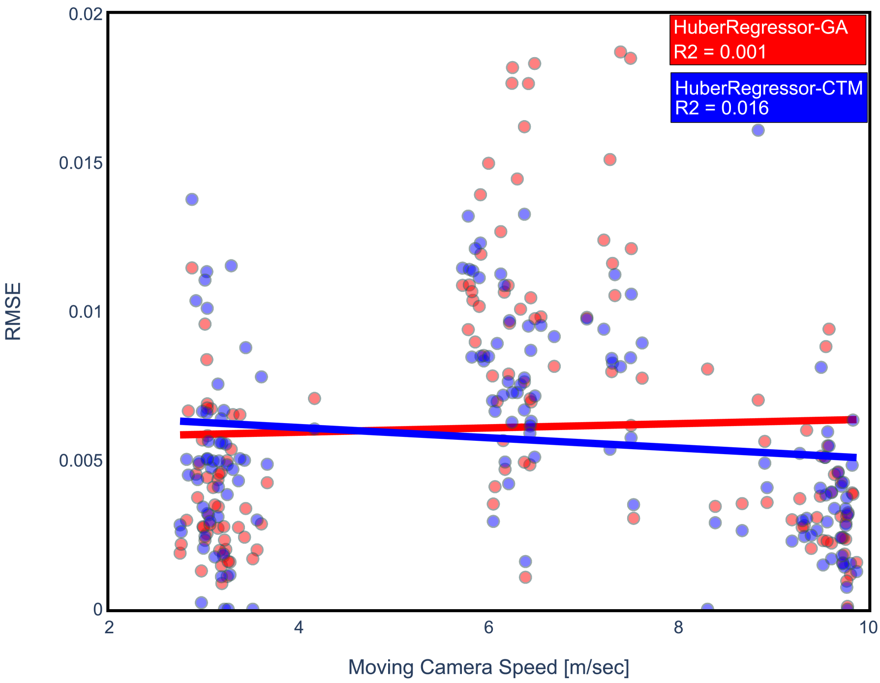
(b) RMSE vs Link speed

Figure 16: Variation in RMSE with change in average density on the opposite link and moving camera speed for all 140 scenarios. The red points corresponds to the RMSE calculated using GA output and blue points corresponds to RMSE calculated using CTM output.

Based on the aforementioned analysis, it can be inferred that the proposed TSE method, which estimates FD parameters and boundary conditions, is capable of generating density cell values that closely approximate the ground truth values, with only a small margin of error. The distribution of RMSE values obtained from the GA outputs closely resembles that of the CTM outputs with known values. This suggests that the main source of error in the GA results can be attributed to the CTM formulation and the process of aggregation, rather than the GA itself.

To a minor extent, deviations from actual initial densities can generate an overall increase of RMSE due to error propagation. Fig. 17 provides an example where the green highlighted cell, generated by the GA, significantly deviates from the actual data.

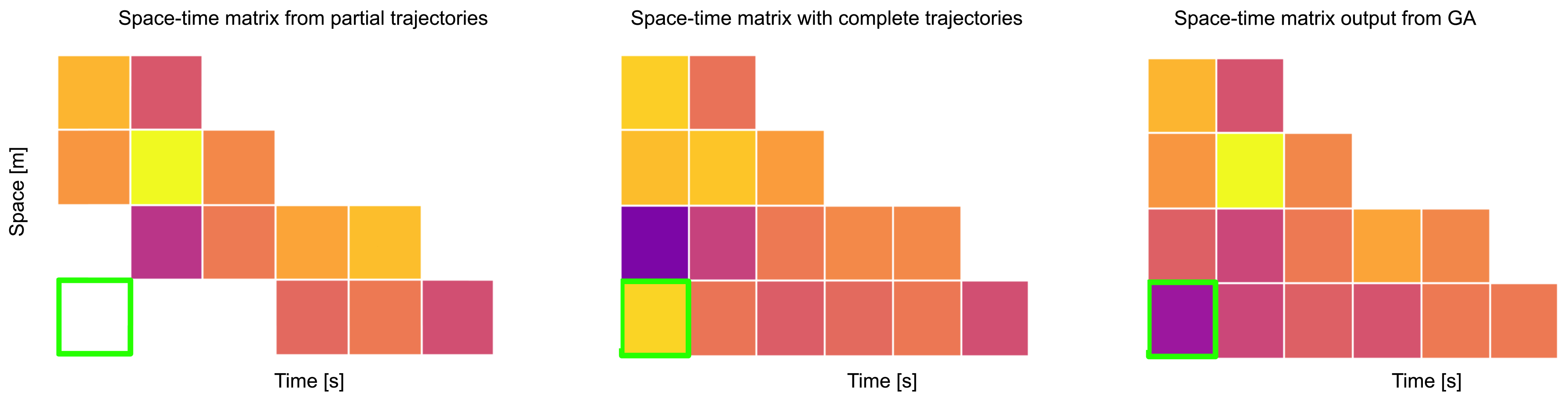
Figure 17: Illustration with an example of deviations from initial density highlighted by ”green” box which leads to error propagation in other cells.

5 Conclusions

This paper introduces a novel approach to link-based TSE by utilizing space-time diagrams derived from street-view video sequences captured by a camera mounted on a moving vehicle. The proposed methodology combines the Genetic Algorithm (GA) procedure to estimate the parameters required for the link’s Fundamental Diagram (FD) and the boundary conditions needed for the Cell Transmission Model (CTM) to estimate densities in unobserved space-time regions. The use of space-time diagrams for traffic measurement offers several advantages over traditional sensors, including higher spatial resolution along the link and the elimination of the need for prior knowledge of the traffic penetration rate during analysis.

The evaluation results, obtained from simulated data generated by the SUMO traffic simulator, provide strong evidence supporting the effectiveness of our proposed methodology in accurately estimating both the FD parameters and boundary conditions. The proposed method achieves a low Root Mean Square Error (RMSE) value of 0.0079 veh/m/cell with a standard deviation of 0.0043 using a space and time cell dimension of 20 m and 2 sec, respectively. Furthermore, the proposed method successfully calibrates the FD parameters with minimal differences of 0.036 m/s in free-flow speed and 0.0045 veh/m in optimal density value. It should be noted that these errors mainly stem from the discretization process and the limited amount of input data used for estimation in the GA. Despite these challenges, the simplicity of the CTM employed yields satisfactory results. However, to further improve the estimation procedure, alternative CTM methods that do not assume cell homogeneity or rely on discrete cells can be explored.

Notation

Notation in article Variable Definition Unit $x$ space m $t$ time sec $k$ density veh/m $k_{c}$ optimal density veh/m $k_{j}$ jam density veh/m $v_{f}$ free flow speed m/sec $w_{c}$ backward wave speed m/sec $Q$ vehicle flow veh/m $L$ total link length m $T$ total time sec $\alpha$ total number of discrete space cells - $\beta$ total number of discrete time cells - $s_{min}$ minimum headway distance m $fov$ camera field of view m

6 References

Appendix A GA parameter search for FD estimation

In order to find the best set of GA parameters that can maximize Root Mean Square Value (RMSE) for $194$ different density quartets from 140 traffic scenarios, we ran a grid search on them. Using a fixed population size of $56$ and crossover fraction of $20$, the rest of the value are varied as follows. This results in total $60$ set of GA parameters.

• Generations = [20, 40, 60, 80, 100]

• k-tournament size = [2, 5, 7, 10]

• Adaptive mutation = [(0.9, 0.1), (0.75, 0.25), (0.5, 0.5)]

In Fig. 18 shows the variation in RMSE for different k-Tournament, Generation and Mutation values. Each plot the variation in RMSE with generation and k-tournament value with fix mutation value. For the analysis, finally the following values were chosen for the evaluation in the experiments: generations = $100$, k-tournament = $5$, adaptive mutation probabilities = $(0.65,0.35)$ and crossover fraction = $20$.

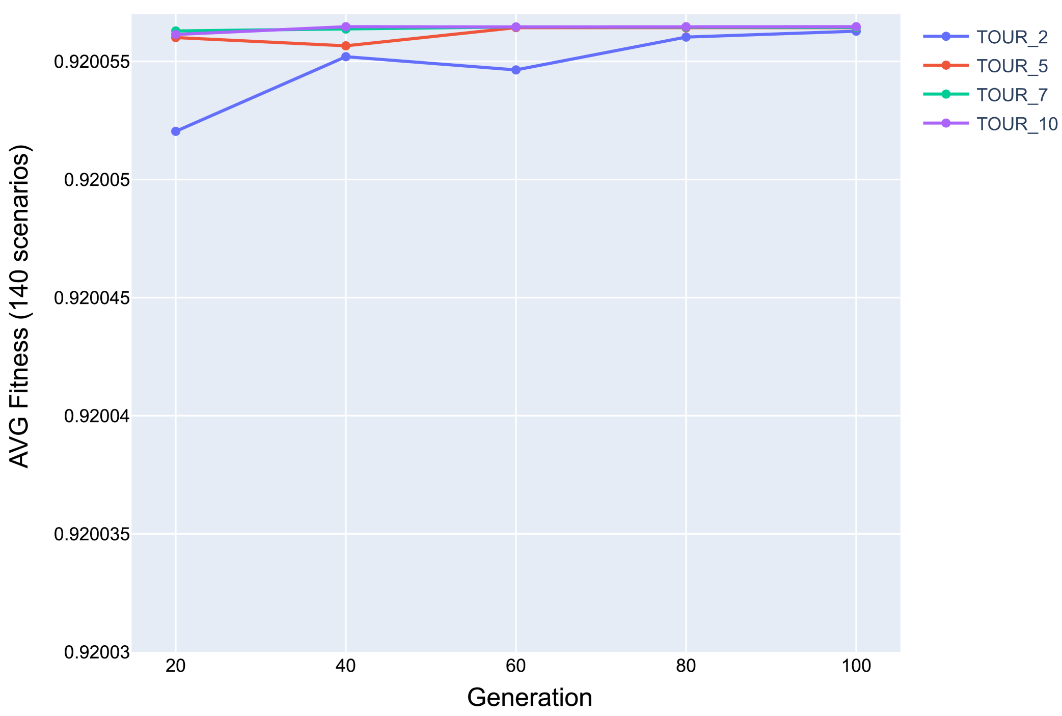
(a) Mutation=(0.5, 0.5)

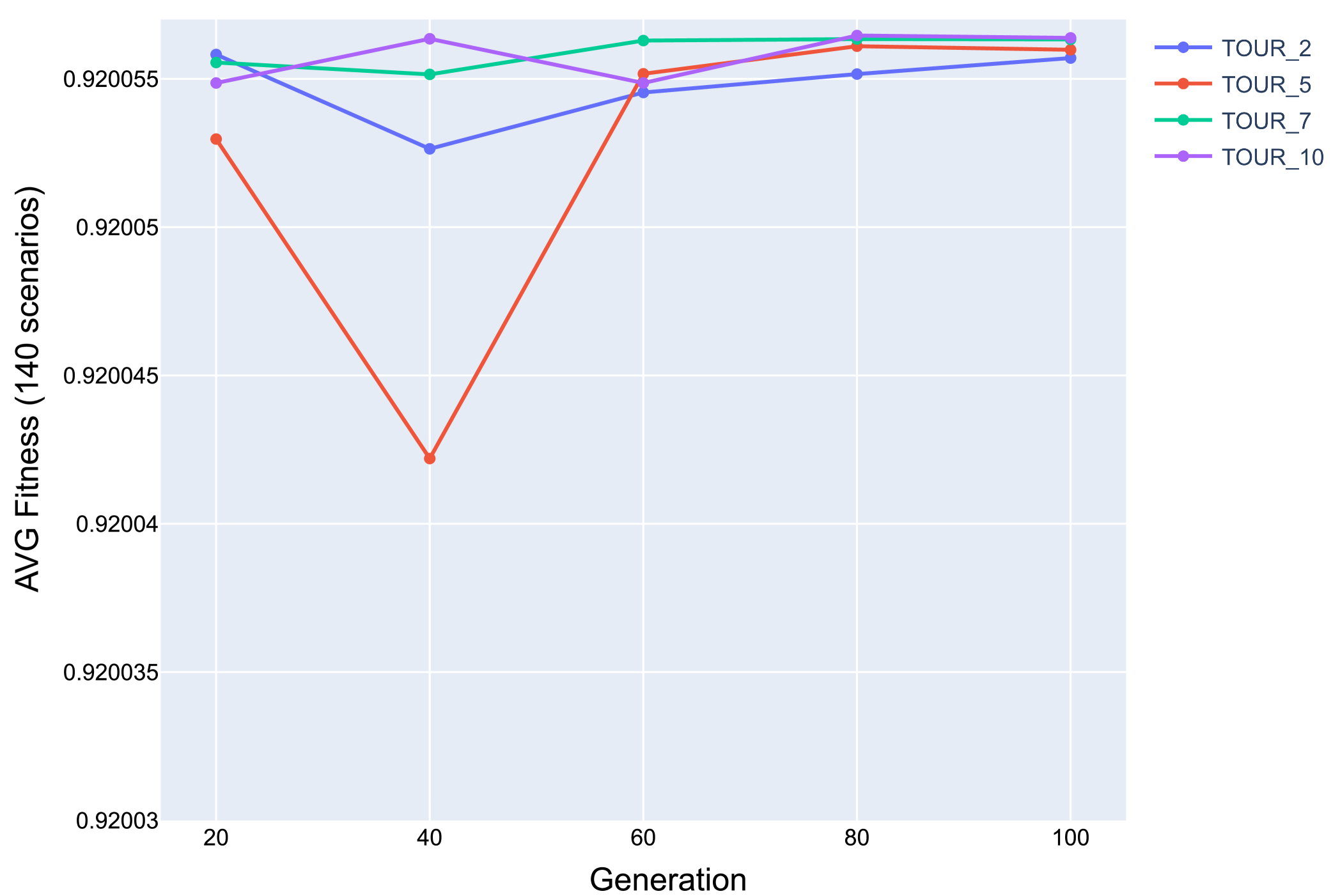
(b) Mutation=(0.75, 0.25)

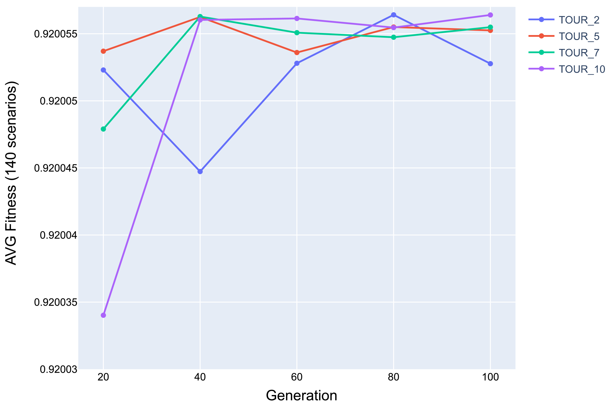
(c) Mutation=(0.9, 0.1)

Figure 18: GA parameter search for varying mutation, k-tournament and generation.

Appendix B GA parameter search for Density estimation

We ran a grid search to find the best set of GA parameters that results in the highest fitness value compared to partial data for all 140 scenarios. We did the search in two parts - varying across k-tournament selection value and mutation probabilities keeping all parameter fixed and later varying generation and population with all other parameter fixed.

For the first run, we use Generation = $60$, Population = $500$ and Crossover fraction = $250$. The other parameter values are varied as follows, resulting in $25$ set of GA parameters.

• K-tournament selection = [2, 4, 6, 8, 10]

• Mutation probabilities = [(0.9, 0.1), (0.8, 0.2), (0.7, 0.3), (0.6, 0.4), (0.5, 0.5)]

For the next run, we use Mutation = $(0.9,0.1)$ and k-tournament = $10$. the crossover fraction is fixed as half of population. The other parameter values are varied as follows, resulting in $25$ set of GA parameters.

• Population = [100, 200, 400, 600, 800]

• Generation = [40, 60, 80, 100, 120]

Fig.19 presents the result of the parameter search across all 140 traffic space-time diagrams. The figure to left shows the increase in fitness with both increase in mutation values and k-tournament size. Similarly, the figure to right shows increase of fitness level with increase in population and generation. For the analysis, finally the following values were chosen for the evaluation in the experiments: generations = 60, population size = 500, k-Tournament = 10, adaptive mutation probabilities = (0.9, 0.1), and crossover fraction = 50.

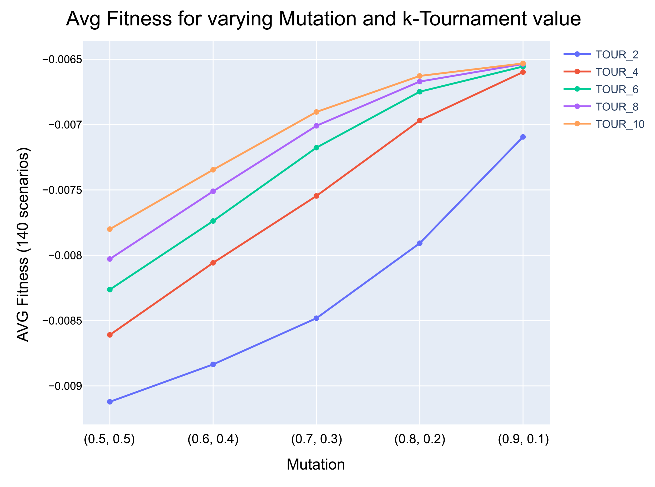
(a) Fitness vs Mutation

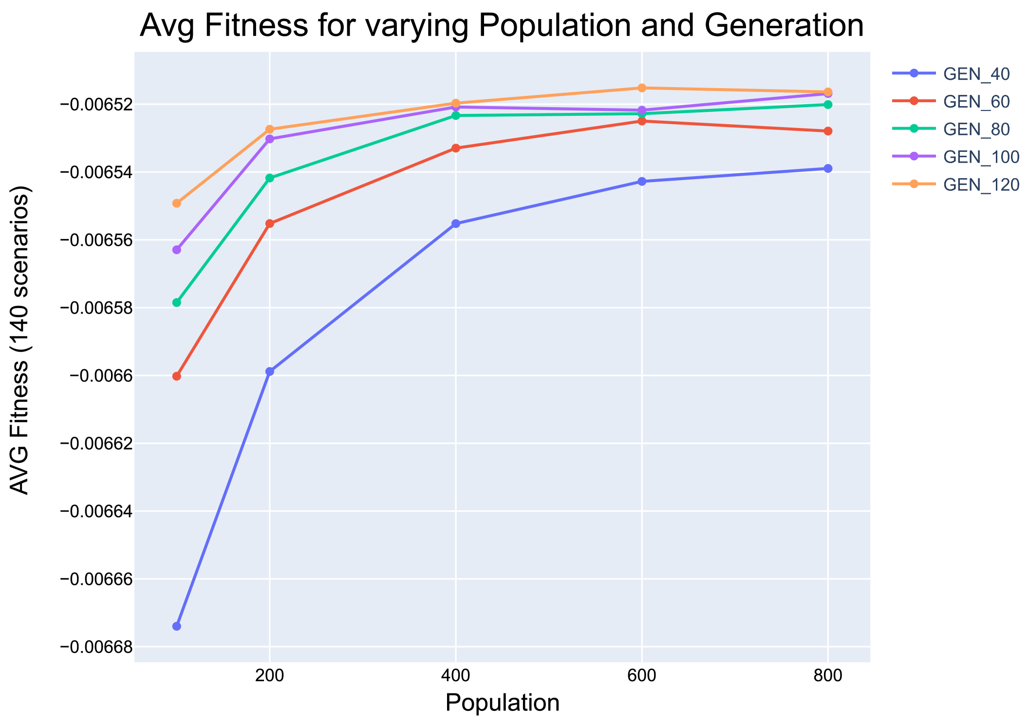
(b) Fitness vs Population

Figure 19: GA parameter search for varying mutation/k-tournament and population/generation.

References

- Coifman \BBA Kim (\APACyear2009) \APACinsertmetastarCoifman2009{APACrefauthors}Coifman, B.\BCBT \BBA Kim, S. \APACrefYearMonthDay20098. \BBOQ\APACrefatitleSpeed estimation and length based vehicle classification from freeway single-loop detectors Speed estimation and length based vehicle classification from freeway single-loop detectors.\BBCQ \APACjournalVolNumPagesTransportation Research Part C: Emerging Technologies174349–364. {APACrefURL} https://linkinghub.elsevier.com/retrieve/pii/S0968090X09000072 {APACrefDOI} 10.1016/j.trc.2009.01.004 \PrintBackRefs\CurrentBib
- Daganzo (\APACyear1994) \APACinsertmetastarDaganzo1994{APACrefauthors}Daganzo, C\BPBIF. \APACrefYearMonthDay19948. \BBOQ\APACrefatitleThe cell transmission model: A dynamic representation of highway traffic consistent with the hydrodynamic theory The cell transmission model: A dynamic representation of highway traffic consistent with the hydrodynamic theory.\BBCQ \APACjournalVolNumPagesTransportation Research Part B: Methodological284269–287. {APACrefURL} https://linkinghub.elsevier.com/retrieve/pii/0191261594900027 {APACrefDOI} 10.1016/0191-2615(94)90002-7 \PrintBackRefs\CurrentBib
- Edie (\APACyear1963) \APACinsertmetastarEdie1963{APACrefauthors}Edie, L. \APACrefYearMonthDay1963. \BBOQ\APACrefatitleDiscussion of Traffic Stream Measurements and Definitions Discussion of Traffic Stream Measurements and Definitions.\BBCQ \BIn \APACrefbtitle2nd International Symposium on the Theory of Traffic Flow. 2nd international symposium on the theory of traffic flow. \PrintBackRefs\CurrentBib
- Geiger \BOthers. (\APACyear2012) \APACinsertmetastarKITTI{APACrefauthors}Geiger, A., Lenz, P.\BCBL \BBA Urtasun, R. \APACrefYearMonthDay2012. \BBOQ\APACrefatitleAre we ready for autonomous driving? the KITTI vision benchmark suite Are we ready for autonomous driving? the KITTI vision benchmark suite.\BBCQ \BIn \APACrefbtitleProceedings of the IEEE Computer Society Conference on Computer Vision and Pattern Recognition Proceedings of the ieee computer society conference on computer vision and pattern recognition (\BPGS 3354–3361). {APACrefDOI} 10.1109/CVPR.2012.6248074 \PrintBackRefs\CurrentBib
- Herrera \BBA Bayen (\APACyear2010) \APACinsertmetastarHerrera2010{APACrefauthors}Herrera, J\BPBIC.\BCBT \BBA Bayen, A\BPBIM. \APACrefYearMonthDay2010. \BBOQ\APACrefatitleIncorporation of Lagrangian measurements in freeway traffic state estimation Incorporation of Lagrangian measurements in freeway traffic state estimation.\BBCQ \APACjournalVolNumPagesTransportation Research Part B: Methodological444460–481. {APACrefDOI} 10.1016/j.trb.2009.10.005 \PrintBackRefs\CurrentBib
- John H. Holland (\APACyear1992) \APACinsertmetastarJohnHolland1992{APACrefauthors}John H. Holland. \APACrefYear1992. \APACrefbtitleAdaptation in Natural and Artificial Systems: An Introductory Analysis with Applications to Biology, Control, and Artificial Intelligence Adaptation in Natural and Artificial Systems: An Introductory Analysis with Applications to Biology, Control, and Artificial Intelligence (\PrintOrdinal1 \BEd, \BVOL 1). \APACaddressPublisherMIT Press. {APACrefURL} https://ieeexplore.ieee.org/servlet/opac?bknumber=6267401 \PrintBackRefs\CurrentBib
- Katoch \BOthers. (\APACyear2021) \APACinsertmetastarKatoch2021{APACrefauthors}Katoch, S., Chauhan, S\BPBIS.\BCBL \BBA Kumar, V. \APACrefYearMonthDay20212. \BBOQ\APACrefatitleA review on genetic algorithm: past, present, and future A review on genetic algorithm: past, present, and future.\BBCQ \APACjournalVolNumPagesMultimedia Tools and Applications8058091–8126. {APACrefURL} http://link.springer.com/10.1007/s11042-020-10139-6 {APACrefDOI} 10.1007/s11042-020-10139-6 \PrintBackRefs\CurrentBib
- Kumar \BOthers. (\APACyear2021) \APACinsertmetastarKumar2021{APACrefauthors}Kumar, A., Kashiyama, T., Maeda, H.\BCBL \BBA Sekimoto, Y. \APACrefYearMonthDay202112. \BBOQ\APACrefatitleCitywide reconstruction of cross-sectional traffic flow from moving camera videos Citywide reconstruction of cross-sectional traffic flow from moving camera videos.\BBCQ \BIn \APACrefbtitle2021 IEEE International Conference on Big Data (Big Data) 2021 ieee international conference on big data (big data) (\BPGS 1670–1678). \APACaddressPublisherIEEE. {APACrefURL} https://ieeexplore.ieee.org/document/9671751/ {APACrefDOI} 10.1109/BigData52589.2021.9671751 \PrintBackRefs\CurrentBib
- X. Li \BOthers. (\APACyear2013) \APACinsertmetastarLi2013{APACrefauthors}Li, X., She, Y., Luo, D.\BCBL \BBA Yu, Z. \APACrefYearMonthDay201311. \BBOQ\APACrefatitleA Traffic State Detection Tool for Freeway Video Surveillance System A Traffic State Detection Tool for Freeway Video Surveillance System.\BBCQ \APACjournalVolNumPagesProcedia - Social and Behavioral Sciences962453–2461. {APACrefURL} https://linkinghub.elsevier.com/retrieve/pii/S1877042813024002 {APACrefDOI} 10.1016/j.sbspro.2013.08.274 \PrintBackRefs\CurrentBib
- Y. Li \BOthers. (\APACyear2018) \APACinsertmetastarLi2018{APACrefauthors}Li, Y., Martínez Mori, J\BPBIC.\BCBL \BBA Work, D\BPBIB. \APACrefYearMonthDay201811. \BBOQ\APACrefatitleEstimating traffic conditions from smart work zone systems Estimating traffic conditions from smart work zone systems.\BBCQ \APACjournalVolNumPagesJournal of Intelligent Transportation Systems: Technology, Planning, and Operations226490–502. {APACrefDOI} 10.1080/15472450.2018.1438274 \PrintBackRefs\CurrentBib
- Lighthill \BBA Whitham (\APACyear1955) \APACinsertmetastarLighthill1955{APACrefauthors}Lighthill, M\BPBIJ.\BCBT \BBA Whitham, G\BPBIB. \APACrefYearMonthDay19555. \BBOQ\APACrefatitleOn kinematic waves II. A theory of traffic flow on long crowded roads On kinematic waves II. A theory of traffic flow on long crowded roads.\BBCQ \APACjournalVolNumPagesProceedings of the Royal Society of London. Series A. Mathematical and Physical Sciences2291178317–345. {APACrefURL} https://royalsocietypublishing.org/doi/10.1098/rspa.1955.0089 {APACrefDOI} 10.1098/rspa.1955.0089 \PrintBackRefs\CurrentBib
- Lopez \BOthers. (\APACyear2018) \APACinsertmetastarLopez2018{APACrefauthors}Lopez, P\BPBIA., Wiessner, E., Behrisch, M., Bieker-Walz, L., Erdmann, J., Flotterod, Y\BHBIP.\BDBLWagner, P. \APACrefYearMonthDay201811. \BBOQ\APACrefatitleMicroscopic Traffic Simulation using SUMO Microscopic Traffic Simulation using SUMO.\BBCQ \BIn \APACrefbtitle2018 21st International Conference on Intelligent Transportation Systems (ITSC) 2018 21st international conference on intelligent transportation systems (itsc) (\BPGS 2575–2582). \APACaddressPublisherIEEE. {APACrefURL} https://ieeexplore.ieee.org/document/8569938/ {APACrefDOI} 10.1109/ITSC.2018.8569938 \PrintBackRefs\CurrentBib
- Marsili Libelli \BBA Alba (\APACyear2000) \APACinsertmetastarMarsiliLibelli2000{APACrefauthors}Marsili Libelli, S.\BCBT \BBA Alba, P. \APACrefYearMonthDay20007. \BBOQ\APACrefatitleAdaptive mutation in genetic algorithms Adaptive mutation in genetic algorithms.\BBCQ \APACjournalVolNumPagesSoft Computing4276–80. {APACrefURL} http://link.springer.com/10.1007/s005000000042 {APACrefDOI} 10.1007/s005000000042 \PrintBackRefs\CurrentBib
- Munoz \BOthers. (\APACyear2004) \APACinsertmetastarMunoz2004{APACrefauthors}Munoz, L., Xiaotian Sun, Dengfeng Sun, Gomes, G.\BCBL \BBA Horowitz, R. \APACrefYearMonthDay2004. \BBOQ\APACrefatitleMethodological calibration of the cell transmission model Methodological calibration of the cell transmission model.\BBCQ \BIn \APACrefbtitleProceedings of the 2004 American Control Conference Proceedings of the 2004 american control conference (\BVOL 1, \BPGS 798–803). \APACaddressPublisherIEEE. {APACrefURL} https://ieeexplore.ieee.org/document/1383703/ {APACrefDOI} 10.23919/ACC.2004.1383703 \PrintBackRefs\CurrentBib
- Panda \BOthers. (\APACyear2019) \APACinsertmetastarPanda2019{APACrefauthors}Panda, M., Ngoduy, D.\BCBL \BBA Vu, H\BPBIL. \APACrefYearMonthDay20198. \BBOQ\APACrefatitleMultiple model stochastic filtering for traffic density estimation on urban arterials Multiple model stochastic filtering for traffic density estimation on urban arterials.\BBCQ \APACjournalVolNumPagesTransportation Research Part B: Methodological126280–306. {APACrefDOI} 10.1016/j.trb.2019.06.009 \PrintBackRefs\CurrentBib
- Pletzer \BOthers. (\APACyear2012) \APACinsertmetastarPletzer2012{APACrefauthors}Pletzer, F., Tusch, R., Böszörmenyi, L.\BCBL \BBA Rinner, B. \APACrefYearMonthDay2012. \BBOQ\APACrefatitleRobust traffic state estimation on smart cameras Robust traffic state estimation on smart cameras.\BBCQ \BIn \APACrefbtitleProceedings - 2012 IEEE 9th International Conference on Advanced Video and Signal-Based Surveillance, AVSS 2012 Proceedings - 2012 ieee 9th international conference on advanced video and signal-based surveillance, avss 2012 (\BPGS 434–439). {APACrefDOI} 10.1109/AVSS.2012.63 \PrintBackRefs\CurrentBib
- Rastogi \BBA Björkman (\APACyear2023) \APACinsertmetastarTanay2023{APACrefauthors}Rastogi, T.\BCBT \BBA Björkman, M. \APACrefYearMonthDay2023. \APACrefbtitleAutomated Construction of Time-Space Diagrams for Traffic Analysis Using Street-View Video Sequence. Automated construction of time-space diagrams for traffic analysis using street-view video sequence. {APACrefURL} https://doi.org/10.48550/arXiv.2308.06098 \PrintBackRefs\CurrentBib
- Richards (\APACyear1956) \APACinsertmetastarRichards1956{APACrefauthors}Richards, P\BPBII. \APACrefYearMonthDay19562. \BBOQ\APACrefatitleShock Waves on the Highway Shock Waves on the Highway.\BBCQ \APACjournalVolNumPagesOperations Research4142–51. {APACrefURL} http://pubsonline.informs.org/doi/10.1287/opre.4.1.42 {APACrefDOI} 10.1287/opre.4.1.42 \PrintBackRefs\CurrentBib
- Robinson \BBA Polak (\APACyear2005) \APACinsertmetastarRobinson2005{APACrefauthors}Robinson, S.\BCBT \BBA Polak, J\BPBIW. \APACrefYearMonthDay20051. \BBOQ\APACrefatitleModeling Urban Link Travel Time with Inductive Loop Detector Data by Using the k-NN Method Modeling Urban Link Travel Time with Inductive Loop Detector Data by Using the k-NN Method.\BBCQ \APACjournalVolNumPagesTransportation Research Record: Journal of the Transportation Research Board1935147–56. {APACrefURL} http://journals.sagepub.com/doi/10.1177/0361198105193500106 {APACrefDOI} 10.1177/0361198105193500106 \PrintBackRefs\CurrentBib
- Seo \BOthers. (\APACyear2017) \APACinsertmetastarSeo2017{APACrefauthors}Seo, T., Bayen, A\BPBIM., Kusakabe, T.\BCBL \BBA Asakura, Y. \APACrefYearMonthDay2017. \BBOQ\APACrefatitleTraffic state estimation on highway: A comprehensive survey Traffic state estimation on highway: A comprehensive survey.\BBCQ \BIn \APACrefbtitleAnnual Reviews in Control Annual reviews in control (\BVOL 43, \BPGS 128–151). \APACaddressPublisherElsevier Ltd. {APACrefDOI} 10.1016/j.arcontrol.2017.03.005 \PrintBackRefs\CurrentBib
- Seo \BOthers. (\APACyear2015\APACexlab\BCnt1) \APACinsertmetastarSeo2015PV{APACrefauthors}Seo, T., Kusakabe, T.\BCBL \BBA Asakura, Y. \APACrefYearMonthDay2015\BCnt14. \BBOQ\APACrefatitleEstimation of flow and density using probe vehicles with spacing measurement equipment Estimation of flow and density using probe vehicles with spacing measurement equipment.\BBCQ \APACjournalVolNumPagesTransportation Research Part C: Emerging Technologies53134–150. {APACrefDOI} 10.1016/j.trc.2015.01.033 \PrintBackRefs\CurrentBib
- Seo \BOthers. (\APACyear2015\APACexlab\BCnt2) \APACinsertmetastarSeo2015TSE{APACrefauthors}Seo, T., Kusakabe, T.\BCBL \BBA Asakura, Y. \APACrefYearMonthDay2015\BCnt210. \BBOQ\APACrefatitleTraffic State Estimation with the Advanced Probe Vehicles Using Data Assimilation Traffic State Estimation with the Advanced Probe Vehicles Using Data Assimilation.\BBCQ \BIn \APACrefbtitleIEEE Conference on Intelligent Transportation Systems, Proceedings, ITSC Ieee conference on intelligent transportation systems, proceedings, itsc (\BVOL 2015-October, \BPGS 824–830). \APACaddressPublisherInstitute of Electrical and Electronics Engineers Inc. {APACrefDOI} 10.1109/ITSC.2015.139 \PrintBackRefs\CurrentBib
- Sumalee \BOthers. (\APACyear2011) \APACinsertmetastarSumalee2011{APACrefauthors}Sumalee, A., Zhong, R., Pan, T.\BCBL \BBA Szeto, W. \APACrefYearMonthDay20113. \BBOQ\APACrefatitleStochastic cell transmission model (SCTM): A stochastic dynamic traffic model for traffic state surveillance and assignment Stochastic cell transmission model (SCTM): A stochastic dynamic traffic model for traffic state surveillance and assignment.\BBCQ \APACjournalVolNumPagesTransportation Research Part B: Methodological453507–533. {APACrefURL} https://linkinghub.elsevier.com/retrieve/pii/S0191261510001189 {APACrefDOI} 10.1016/j.trb.2010.09.006 \PrintBackRefs\CurrentBib
- Sunderrajan \BOthers. (\APACyear2016) \APACinsertmetastarSunderrajan2016{APACrefauthors}Sunderrajan, A., Viswanathan, V., Cai, W.\BCBL \BBA Knoll, A. \APACrefYearMonthDay2016. \BBOQ\APACrefatitleTraffic state estimation using floating car data Traffic state estimation using floating car data.\BBCQ \BIn \APACrefbtitleProcedia Computer Science Procedia computer science (\BVOL 80, \BPGS 2008–2018). \APACaddressPublisherElsevier B.V. {APACrefDOI} 10.1016/j.procs.2016.05.521 \PrintBackRefs\CurrentBib
- Takenouchi \BOthers. (\APACyear2019) \APACinsertmetastarTakenouchi2019{APACrefauthors}Takenouchi, A., Kawai, K.\BCBL \BBA Kuwahara, M. \APACrefYearMonthDay20197. \BBOQ\APACrefatitleTraffic state estimation and its sensitivity utilizing measurements from the opposite lane Traffic state estimation and its sensitivity utilizing measurements from the opposite lane.\BBCQ \APACjournalVolNumPagesTransportation Research Part C: Emerging Technologies10495–109. {APACrefDOI} 10.1016/j.trc.2019.04.016 \PrintBackRefs\CurrentBib
- Tampere \BBA Immers (\APACyear2007) \APACinsertmetastarTampere2007{APACrefauthors}Tampere, C\BPBIM.\BCBT \BBA Immers, L\BPBIH. \APACrefYearMonthDay20079. \BBOQ\APACrefatitleAn Extended Kalman Filter Application for Traffic State Estimation Using CTM with Implicit Mode Switching and Dynamic Parameters An Extended Kalman Filter Application for Traffic State Estimation Using CTM with Implicit Mode Switching and Dynamic Parameters.\BBCQ \BIn \APACrefbtitle2007 IEEE Intelligent Transportation Systems Conference 2007 ieee intelligent transportation systems conference (\BPGS 209–216). \APACaddressPublisherIEEE. {APACrefURL} http://ieeexplore.ieee.org/document/4357755/ {APACrefDOI} 10.1109/ITSC.2007.4357755 \PrintBackRefs\CurrentBib
- Timotheou \BOthers. (\APACyear2015) \APACinsertmetastarTimotheou2015{APACrefauthors}Timotheou, S., Panayiotou, C\BPBIG.\BCBL \BBA Polycarpou, M\BPBIM. \APACrefYearMonthDay201512. \BBOQ\APACrefatitleMoving horizon fault-tolerant traffic state estimation for the Cell Transmission Model Moving horizon fault-tolerant traffic state estimation for the Cell Transmission Model.\BBCQ \BIn \APACrefbtitle2015 54th IEEE Conference on Decision and Control (CDC) 2015 54th ieee conference on decision and control (cdc) (\BPGS 3451–3456). \APACaddressPublisherIEEE. {APACrefURL} http://ieeexplore.ieee.org/document/7402753/ {APACrefDOI} 10.1109/CDC.2015.7402753 \PrintBackRefs\CurrentBib
- Tyagi \BOthers. (\APACyear2012) \APACinsertmetastarTyagi2012{APACrefauthors}Tyagi, V., Kalyanaraman, S.\BCBL \BBA Krishnapuram, R. \APACrefYearMonthDay20124. \BBOQ\APACrefatitleVehicular Traffic Density State Estimation Based on Cumulative Road Acoustics Vehicular Traffic Density State Estimation Based on Cumulative Road Acoustics.\BBCQ \APACjournalVolNumPagesIEEE Transactions on Intelligent Transportation Systems1331156–1166. {APACrefDOI} 10.1109/tits.2012.2190509 \PrintBackRefs\CurrentBib
- Ua-Areemitr \BOthers. (\APACyear2019) \APACinsertmetastarUa-Areemitr2019{APACrefauthors}Ua-Areemitr, E., Sumalee, A.\BCBL \BBA Lam, W\BPBIH. \APACrefYearMonthDay20199. \BBOQ\APACrefatitleLow-Cost Road Traffic State Estimation System Using Time-Spatial Image Processing Low-Cost Road Traffic State Estimation System Using Time-Spatial Image Processing.\BBCQ \APACjournalVolNumPagesIEEE Intelligent Transportation Systems Magazine11369–79. {APACrefDOI} 10.1109/MITS.2019.2919634 \PrintBackRefs\CurrentBib
- Van Erp \BOthers. (\APACyear2017) \APACinsertmetastarVanErp2017{APACrefauthors}Van Erp, P\BPBIB., Knoop, V\BPBIL.\BCBL \BBA Hoogendoorn, S\BPBIP. \APACrefYearMonthDay2017. \BBOQ\APACrefatitleMacroscopic Traffic State Estimation: Understanding Traffic Sensing Data-Based Estimation Errors Macroscopic Traffic State Estimation: Understanding Traffic Sensing Data-Based Estimation Errors.\BBCQ \APACjournalVolNumPagesJournal of Advanced Transportation2017. {APACrefDOI} 10.1155/2017/5730648 \PrintBackRefs\CurrentBib
- Yuan \BOthers. (\APACyear2021) \APACinsertmetastarYuan2021{APACrefauthors}Yuan, Y., Zhang, W., Yang, X., Liu, Y., Liu, Z.\BCBL \BBA Wang, W. \APACrefYearMonthDay2021. \BBOQ\APACrefatitleTraffic state classification and prediction based on trajectory data Traffic state classification and prediction based on trajectory data.\BBCQ \APACjournalVolNumPagesJournal of Intelligent Transportation Systems: Technology, Planning, and Operations. {APACrefDOI} 10.1080/15472450.2021.1955210 \PrintBackRefs\CurrentBib