Finding Influencers in Complex Networks: An Effective Deep Reinforcement Learning Approach

Abstract

Maximizing influences in complex networks is a practically important but computationally challenging task for social network analysis, due to its NP-hard nature. Most current approximation or heuristic methods either require tremendous human design efforts or achieve unsatisfying balances between effectiveness and efficiency. Recent machine learning attempts only focus on speed but lack performance enhancement. In this paper, different from previous attempts, we propose an effective deep reinforcement learning model that achieves superior performances over traditional best influence maximization algorithms. Specifically, we design an end-to-end learning framework that combines graph neural network as the encoder and reinforcement learning as the decoder, named DREIM. Through extensive training on small synthetic graphs, DREIMoutperforms the state-of-the-art baseline methods on very large synthetic and real-world networks on solution quality, and we also empirically show its linear scalability with regard to the network size, which demonstrates its superiority in solving this problem.

1 Introduction

Social networks refer to a relatively stable system formed by various interactive relationships among individual members of society. Influence maximization problem is an important issue for social networks analysis, which has wide spread application in practice, including word-of-mouth marketing, crowd mobilization and public opinion monitoring [1, 2]. This problem can be formally described as finding out $k$ seeds (influencers) to maximize their influences under certain propagation model, e.g., the independent cascade model (IC) or the linear threshold model (LT) [3].

Traditional attempts towards this problem can be categorized into two types [4, 5, 6, 7, 8, 9, 10, 11, 12, 13, 14, 15, 16, 17, 18, 19, 20, 21, 22, 23, 3, 24, 25, 26, 27]. First are approximate algorithms [20, 21, 22, 23], which are bounded with theoretical guarantees, and can be applied to medium sized graphs. However the design of these algorithms often requires extensive expert error-and-trials and their scalability often suffers. Second ones are heuristic methods, including random heuristics  [3], evolution-based ones [24], e.g., genetic algorithms, centrality-based ones [25, 26] and degree discount heuristics [27]. These methods are often fast and easy to design, and they can usually produce a feasible solution in a short time.They do not, however, offer any theoretical assurances, and the quality of the solutions can be very poor in some circumstances. Note that both approximate and heuristic methods are ad hoc in nature, with little cross-scenario flexibility.

To our best knowledge, the advantages of data-driven models such as deep reinforcement learning have not been well exploited for tackling the influence maximization problem. Recently, some works have proposed that reinforcement learning can be used to solve the combinatorial optimization problems on graphs [28, 29, 30]. The intuition behind these works is that the model can be trained in a graph distribution $\mathcal{D}$, and the solution set for a new graph can be obtained using the trained model. Dai et al. [28] first implemented this idea. They applied this idea to solve the traditional combinatorial optimization problems such as minimum vertex coverage and maximum coverage problem. However, their method is difficult to apply to large-scale graphs. Later on, this method was improved by Li et al. [30]. Akash et al. [29] first use this idea to solve the problem of influence maximization. Although the calculation speed has been improved, the performance of their algorithm i.e., selecting k seed nodes, and the proportion of nodes finally activated, is not better than the traditional best approximation algorithm IMM. Moreover, their model is trained via supervised learning, however, in real life, providing labels for supervised training is time-consuming and laborious. And supervised training will limit the ability of their model to obtain higher-quality solutions.

Inspired by current existing machine learning attempts in solving combinatorial optimization problems, here, we design DREIM (Deep REinforcement learning for Influence Maximizations), an end-to-end deep reinforcement learning based influence maximization model. More concretely, DREIMincorporates the graph neural network to represent nodes and graphs, and the Q-learning technique to update the trainable parameters. We train DREIMwith large amounts of synthetic graphs, and the learned strategy could be applied on much larger instances, including both synthetic networks and real-world ones. DREIMachieves better solution quality than current state-of-the-art methods, for example, when selecting 100 seed nodes from the Facebook network, DREIMactivates 26700 nodes while IMM activates 20180 nodes. Meanwhile, DREIMcan also be very efficient through a batch nodes selection strategy.

In summary, we make four main contributions:

• We formulate the seed nodes selection process of influence maximization (IM) problem as a Markov decision process.

• We present an end-to-end deep reinforcement learning framework to solve the classical IM problem. We design a novel state representation for reinforcement learning by inducing a virtual node, which can capture system state information more accurately.

• We propose a reasonable and effective termination condition of reinforcement learning, leading to the superior generalization capacity of DREIM.

• We evaluate DREIMthrough extensive experiments on different sizes of large graphs. Our results demonstrate that DREIMis effective and efficient as well as its linear scalability on large networks.

The remaining parts are organized as follows. We systematically review related work in Section 2. After that, we present the preliminaries and problem formalization in Section 3. We then introduce the details of DREIM architecture in Section 4. Section 5 presents the evaluation of DREIMon both large synthetic graphs and real-world networks. In section 6, we first intuitively discuss the policies learned by DREIMand then discuss the effect of our novel Q-learning setting. Finally, we conclude the paper in Section 7.

2 RELATED WORK

2.1 Influence maximization

Domingos and Richardson [31, 32] perform the first study of influence maximization problem, and Kempe et al. [3] first formulate the problem as a discrete optimization problem. Since then influence maximization has been extensively studied [4, 5, 6, 7, 8, 9, 10, 11, 12, 13, 14, 15, 16, 17, 18, 19, 20, 21, 22, 23, 3, 24, 25, 26, 27]. The existing solution methodologies can be classified into three categories.

Approximation methods. Kempe et al. [3] proposed a hill-climbing greedy algorithm with a $1-1/e-\epsilon$ approximation rate, which uses tens of thousands of Monte Carlo simulations to obtain the solution set. Leskovec et al. [20] then proposed a cost-effective delayed forward selection (CELF) algorithm. Experimental results show that the execution time of CELF is 700 times faster than that of the greedy algorithm. Borgs et al. [21] Borgs et al. proposed a IM sampling method called RIS. A threshold is set to determine how many reverse reachable sets are generated by the network and the node that covers the most of these sets is selected. TIM/TIM+ [22] greatly improves the efficiency of [21], and is the first RIS-based approximation algorithm that achieves efficiency comparable to that of heuristic algorithms. Later, IMM [23] employs the concept of martingale to reduce computation time while retaining TIM’s $1-1/e-\epsilon$ approximation guarantee. According to a benchmark study [33], IMM is known as the state-of-the-art approximation algorithm for solving IM problem.In addition, Tang et al. [4] proposed OPIM to improve interactivity and flexibility for a better online user experience. The disadvantages of most approximation methods are that they suffer from scalability problems and rely heavily on expert knowledge.

Heuristic methods. Unlike approximation methods, heuristic don’t give any worst-case bound on the influence spread. These methods include the random heuristic [3], which randomly selects seed nodes; the centrality-based heuristic [25, 26], which selects nodes with high centrality; the evolution-based heuristic [24] and the degree-discounting heuristic proposed by Chen et al. [27] which has similar effectiveness to the greedy algorithm and improves efficiency.

Machine learning methods. Akash et al. [29] first leveraged reinforcement learning method to solve the influence maximization problem. Their model includes a supervised component that uses the greedy algorithm to generate solutions to supervise the neural network. However, generating the training data is a big challenge and supervised learning often suffers from the over-fitting issue.

2.2 Graph representation learning

Graph representation learning (GRL) tries to find $d$-dimensional $(d\ll{|\mathcal{V}|})$ dense vectors to capture the graph information. The obtained vectors can be easily fed to downstream machine learning models to solve various tasks like node classification [34], link prediction [35], graph visualization [36], graph property prediction [37], to name a few. $\mathrm{GNNs}$ are among the most popular graph representation learning methods which adopt a massage passing paradigm [38, 39]. Let $\mathbf{h}_{v}^{(l)}$ denote the embedding vector of node $v$ at layer $l$, a typical $\mathrm{GNN}$ includes two steps: (i) Every node aggregates the embedding vectors from its neighbors at layer $l-1$; (ii) Every node updates its embedding through combining its embedding in last layer and the aggregated neighbor embedding:

$$\mathbf{h}_{\mathcal{N}(v)}^{(l)}=\operatorname{AGGREGATE}\left(\left\{\mathbf{h}_{u}^{(l-1)},\forall u\in\mathcal{N}(v)\right\}\right),$$ (1)

$$\mathbf{h}_{v}^{(l)}=\beta\left(\mathbf{W}^{(l)}\cdot\operatorname{COMBINE}\left(\mathbf{h}_{v}^{(l-1)},\mathbf{h}_{\mathcal{N}(v)}^{(l)}\right)\right),$$ (2)

where $\mathcal{N}(\cdot)$ denotes a set of neighboring nodes of a given node, $W^{(l)}$ is a trainable weight matrix of the $lth$ layer shared by all nodes, and $\beta$ is an activation function, e.g., ReLU.

2.3 Deep reinforcement learning

The reinforcement learning framework [40] considers tasks in which the agent interacts with a dynamic environment through a sequence of observations, actions and rewards. Different from supervised learning, the agent in reinforcement learning is never directly told the best action under certain state, but learns by itself to realize whether its previous sequence of actions are right or not only when an episode ends. The goal of reinforcement learning is to select actions in a fashion that maximizes the long-term performance metric. More formally, it uses a deep neural network to approximate the optimal state-action value function

$$\begin{split}&Q^{*}(s,a)=\\ &\mathrm{max}_{\pi}\mathbb{E}\left[r_{t}+\gamma r_{t+1}+\gamma^{2}r_{t+2}+\ldots\mid s_{t}=s,a_{t}=a,\pi\right],\end{split}$$ (3)

where $\gamma$ is the discounted factor, $\pi=P(a|s)$ is the behaviour policy, which means taking action $a$ at state $s$.

2.4 Machine learning for combinatorial optimization

In a recent survey, Bengio et al. [41] summarize three algorithmic structures for solving combinatorial optimization problems using machine learning: end to end learning that treats the solution generation process as a whole [28, 42, 43], learning to configure algorithms [44, 45], and learning in parallel with optimization algorithms [46, 47]. Dai et al. [28] firstly highlight that it is possible to learn combinatorial algorithms on graphs using deep reinforcement learning. Then, Li et al. [30] and Akash et al. [29] propose improvements from different aspects. Recently, Fan et al. [48] have proposed an deep reinforcement learning framework to solve the key player finding problem on social networks. Most of these algorithms are based on two observations. First, although all kinds of social networks in real life are complex and changeable, the underlying generation models of these networks are unified, such as BA model [49], WS model [50], ER model [51], and powerlaw-cluster model [52], etc. Second, the nodes in the solution set selected by the approximation algorithms should have similar characteristics, such as high betweenness centrality.

3 PRELIMINARIES AND PROBLEM FORMALIZATION

In this section, we first introduce some preliminaries of the influence maximization problem and then give its formalization.

3.1 Preliminaries

Let $\mathcal{G}=(\mathcal{V},\mathcal{E},\mathbf{W})$ be a social network, where $\mathcal{V}$ is a set of nodes (users), $\mathcal{E}$ is a set of edges (relationships), $|\mathcal{V}|=N$ and $|\mathcal{E}|=M$. $(u,v)\in{\mathcal{E}}$ represents an edge from node $u$ to node $v$. Let $\mathbf{W}$ denote the weight matrix of edges indicating the degree of influence. $\mathcal{V}_{a}$ denotes the active nodes set.

• Seed node: A node $v\in{\mathcal{V}}$ that is initially activated as the information source of the entire graph $\mathcal{G}$. The set of seed nodes is denoted by ${\mathcal{S}}$, and $\bar{{\mathcal{S}}}$ is the complementary set of ${\mathcal{S}}$.

• Active node: A node $v\in{\mathcal{V}}$ is regarded as active if it is a seed node ($v\in{{\mathcal{S}}}$) or it is influenced by previously active node $u\in{\mathcal{V}_{a}}$.

• Spread: The expected proportion of activated nodes after the process of influence propagation terminates, denoted as $\sigma({\mathcal{S}})=\frac{|\mathcal{V}_{a}|}{|\mathcal{V}|}$.

• Linear threshold model: LT model simulates the common herd mentality phenomenon in social networks. In this model, each node $v$ in a graph has a threshold $\theta_{v}$. Let $\mathcal{N}(v)$ be the set of neighbors of node $v$ and $\mathcal{N}^{\alpha}(v)$ be the set of activated neighbors of node $v$. For each node $u\in\mathcal{N}(v)$, the edge $(u,v)$ has a non-negative weight $\mathbf{w}(u,v)\leq 1$. Given a graph $\mathcal{G}$ and a seed set ${\mathcal{S}}$, and the threshold for each node, this model first activates the nodes in ${\mathcal{S}}$. Then information starts spreading in discrete timestamps following the following rule. An inactive node $v$ will be activated if $\sum_{u\in\mathcal{N}^{\alpha}(v)}{\mathbf{w}(u,v)}\geq\theta_{v}$. The newly activated nodes attempt to activate their neighbors. This process stops when no new nodes are activated.

3.2 Problem formalization

The influence maximization problem is formally defined as follows:

$$\mathrm{argmax}_{|{\mathcal{S}}|=k,{\mathcal{S}}\subseteq\mathcal{V}}\sigma({\mathcal{S}}),$$ (4)

where ${\mathcal{S}}$ is the solution set, $\sigma$ is the spread calculation function and $k$ is the budget.

We set the threshold of each node as a random real number between $0\sim 1$. And for every node $v\in{\mathcal{V}}$, we set the influence weight of its neighbors as $\frac{1}{|\mathcal{N}_{v}|}$ where $|\mathcal{N}_{v}|$ denotes the number of neighbors of node $v$. To our best knowledge, we are the first who utilize deep learning method to tackle the influence maximization problem under LT diffusion model.

4 PROPOSED MODEL: DREIM

In this section, we introduce the proposed model named DREIM. We begin with the overview and then introduce the architecture by parts as well as the training procedure. We also analyze the time complexity of DREIMin the end of this section.

4.1 Overview

The proposed deep learning model called DREIMcombines graph neural network (GNN) and deep reinforcement learning (DRL) together in an end-to-end manner. As illustrated in Fig. 1, DREIMhas two phases: offline training and online inference. In the offline training phase (top), we train DREIMusing synthetic graphs drawn from a network distribution $\mathcal{D}$, like powerlaw-cluster model adopted here. At first we generate a batch of graphs scaling in a range, like $30\sim 50$. Then we sample one (or a mini-batch) of them as the environment, and let DREIMinteract with it. When the interaction process terminates, the experiences in the form of 4-tuple $\left[S_{i},A_{i},R_{(i,i+n)},S_{(i+n)}\right]$ will be stored in the experience replay buffer with a size of 500000. At the same time, the agent is getting more intelligent by performing mini-batch gradient descents over Eq. $\left(\ref{eq:6}\right)$. During the online inference phase (bottom), we applied the well-trained model to large synthetic and real-world networks with sizes scaling from thousands to millions. In order to decrease the computation time, we adopt a batch nodes selection strategy which selects a batch of highest $Q$-value nodes at each adaptive step. We use the notion DREIM-X to denote different variants of DREIM, where X denotes the number of nodes selected at each step. DREIMrefers to DREIM-1 and DREIM-All means we select k nodes as seed nodes at the very first step.

There are three key parts in DREIM: (i) Encoding, which utilizes the GraphSAGE [39] architecture to learn the nodes’ representations incorporating their structural information and feature information; (ii) Decoding, which generates a scalar $Q$-value for

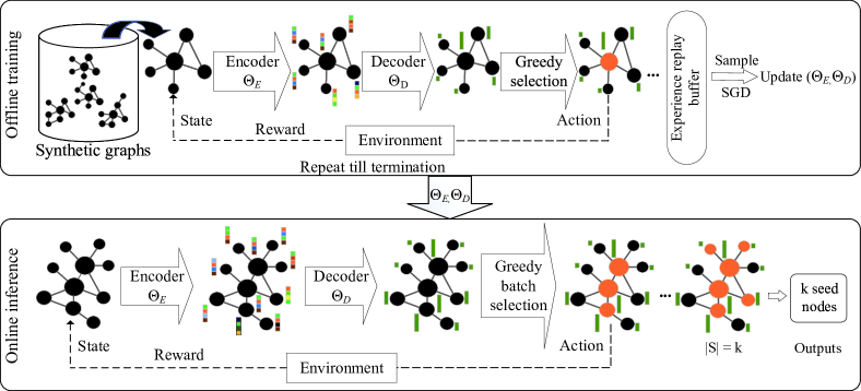
Figure 1: The pipeline of DREIMas a combination of the graph embedding and DQN process. The top half of the figure represents the training phase, and the bottom half is the testing phase. The colour bar denotes each node’s embedding obtained after the encoding process and the green bar shows the Q-value of each node after the 2-layer MLP decoding process. Orange nodes indicate that they have been selected as seed nodes, and black nodes are not selected by DREIM.

each node; (iii) Greedy selection, which adopts the $\epsilon$-greedy strategy in the training phase and the batch nodes selection strategy in the inference phase, to make actions based on the $Q$ values of nodes. In what follows, we will describe each part in detail.

4.2 Encoder

Traditional hand-crafted features, such as node degree centrality, clustering coefficient, etc., can hardly describe the complex nonlinear graph structure. Therefore, we exploit the GraphSAGE [39] architecture to represent complex structure and node attributes using $d$-dimensional dense vectors. Alg. 1 presents the pseudo code of GraphSAGE. The input node attributes vector $\mathbf{X}_{v}$ should include some raw structural information of a node. In this paper, we utilize a 2-tuple [out-degree, isseed] to set the input node attributes, where “out-degree” denotes the summation of outgoing edge weights of node $v$, and “isseed” denotes whether a node $v$ is already selected as seed node, i.e., this feature is set 1 if node $v$ is already a seed node and 0 if node $v$ is not a seed node. For the representation of the entire graph, we use the embedding of a virtual node that has connections to all the nodes in unique direction.

Algorithm 1 Encoding algorithm

0:  $\mathcal{G}=(\mathcal{V},\mathcal{E},\mathbf{W})$; node attributes $\mathbf{X}_{v}\in{\mathbf{R}^{1\times c}},\forall v\in\mathcal{V}\cup\{s\}$; iteration depth $L$; weight parameters $\mathbf{W}_{1}\in\mathbf{R}^{c\times d},\mathbf{W}_{2}\in$ $\mathbf{R}^{d\times(d/2)},\mathbf{W}_{3}\in\mathbf{R}^{d\times(d/2)}$

0:  Embedding vector $\mathbf{z}_{v},\forall v\in\mathcal{V}\cup\{s\}$

1:  Create a virtual node $s$ which connects all nodes in the graph, denoted as the graph state

2:  Initialize $\mathbf{h}_{v}^{(0)}\leftarrow\operatorname{ReLU}\left(\mathbf{X}_{v}\cdot\mathbf{W}_{1}\right),\mathbf{h}_{v}^{(0)}\leftarrow\mathbf{h}_{v}^{(0)}/\left\|\mathbf{h}_{v}^{(0)}\right\|_{2},\forall v\in\mathcal{V}\cup\{s\}$

3:  for $l=1$ to $L$ do

4:     for $v\in{\mathcal{V}}\cup\left\{s\right\}$ do

5:        $\mathbf{h}_{\mathcal{N}(v)}^{(l-1)}\leftarrow\sum_{j\in\mathcal{N}(v)}\mathbf{h}_{j}^{(l-1)}$

6:        $\mathbf{h}_{v}^{(l)}\leftarrow\operatorname{ReLU}\left(\left[\mathbf{W}_{2}\cdot\mathbf{h}_{v}^{(l-1)},\mathbf{W}_{3}\cdot\mathbf{h}_{\mathcal{N}(v)}^{(l-1)}\right]\right)$

7:     end for

8:     $\mathbf{h}_{v}^{(l)}\leftarrow\mathbf{h}_{v}^{(l)}/\left\|\mathbf{h}_{v}^{(l)}\right\|_{2},\forall v\in\mathcal{V}\cup\{s\}$

9:  end for

10:  $\mathbf{z}_{v}\leftarrow\mathbf{h}_{v}^{(K)},\forall v\in\mathcal{V}\cup\{s\}$

4.3 Decoder

In the previous step, we obtain the embeddings, in which the virtual node’s embedding can be regarded as the state while other nodes’ embeddings as the potential actions. In the decoding step, we aim to learn a function that can transfer the state-action pair $\left(s,a\right)$ to a scalar value $Q\left(s,a\right)$. The scalar value indicates the expected maximal rewards after taking action $a$ given state s. In DREIM, the embeddings of state and actions are fed into a 2-layer MLP. We employ rectified linear unit $\left(\mathrm{ReLU}\right)$ as the activation function. Formally, the decoding process can be defined as follows:

$$Q(s,a)=\mathbf{W}_{5}^{\top}\operatorname{ReLU}\left(\mathbf{z}_{a}^{\top}\cdot\mathbf{z}_{s}\cdot\mathbf{W}_{4}\right),$$ (5)

where $\mathbf{W}_{4}\in\mathbf{R}^{d\times 1},\mathbf{W}_{5}\in\mathbf{R}^{d\times 1}$ are weight parameters between two neural network layers, $\mathbf{z}_{s}$ and $\mathbf{z}_{a}\in\mathbf{R}^{1\times d}$ are the output embeddings for state and action respectively. We present how we define the elements of $Q$-learning as follows:

• State: We create a virtual node to represent the state $s$. $s$ updates its embedding in the same way as other nodes do, i.e., message aggregation and combination.

• Action: Action is the process of adding a node $v\notin{{\mathcal{S}}}$ to the solution set ${\mathcal{S}}$.

• Transition: When a node $v$ is selected to join the solution set ${\mathcal{S}}$, the “isseed” attribute of it will change from 0 to 1.

  

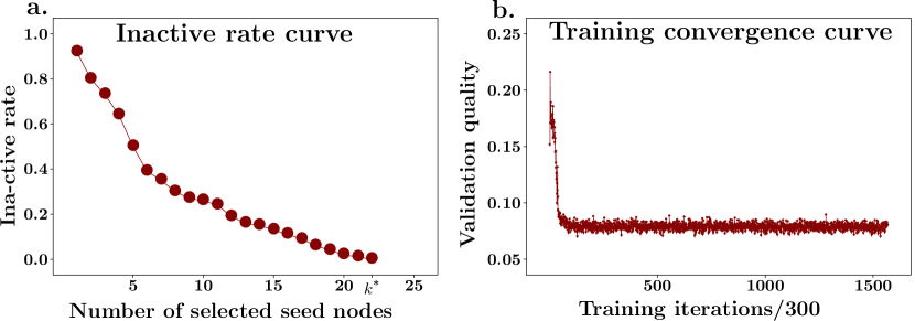
  Figure 2: Training analysis of DREIM. (a). Remaining inactive rate decreases as the number of seed nodes increases. $k^{*}$ seed nodes are selected to activate all the nodes in a network. (b). The training process convergences fast measured by validation quality, i.e., area under the inactive rate curve.

• Reward: After the agent makes an action, it will receive a feedback from the environment, which represents reward or punishment. In DREIM, we use negative inactive rate $-\frac{|\mathcal{V}|-|\mathcal{V}_{a}|}{|\mathcal{V}|}$, i.e., $\sigma-1$ to denote the reward after adding a node into ${\mathcal{S}}$.

• Policy: Policy is the rule the agent obeys to pick the next action. In this work, we adopts different policies during training and inference, and we introduce it concretely in section 4.4

• Termination: The interaction process terminates when all nodes are activated. We choose this termination condition to improve DREIM’s generalization ability. Previous works set the termination condition as $|{\mathcal{S}}|=k$ [29, 53], we argue this will hinder the model’s generalization ability. For example, when the budget $k=10$, there will be 90 nodes left for a graph with 100 nodes, but there will be 990 nodes left for a graph with 1000 nodes, which will confuse the agent, since the terminal state is totally different for graphs with different sizes.

4.4 Greedy Selection

Based on the above two steps, we adopt a greedy selection process to make actions based on the $Q$ values of nodes. In the training phase, since the model has not been trained well, we adopt the $\epsilon$-greedy strategy to balance exploration and exploitation. In the inference phase, since we have already trained DREIMwell, we only exploit the learned $Q$ function to take the highest $Q$ value action. In order to speed up the solution set generation process, we also adopt a batch nodes selection strategy, which takes the top-$k$ nodes with the highest $Q$-value at each adaptive step. Extensive analysis shows that this strategy can bring a significant speed increase without compromising much on solution quality.

Algorithm 2 Training algorithm

0:  number of episodes $e$, replay buffer size $b$,

1:  Initialize DQN $\Theta$ and target DQN $\hat{\Theta}$

2:  Initialize $n$-step experience replay buffer $B$

3:  for episode =1 to $e$ do

4:     Draw random graphs from distribution $D$, like powerlaw-cluster model

5:     Initialize the solution set $S$ as an empty set $\emptyset$

6:     for t=1 to Termination do

7:        Compute embeddings and $Q$ values

8:        c $\leftarrow$ random number between 0 and 1

9:        $v_{t}=\left\{\begin{array}[]{ll}\text{random node }v\in\bar{{\mathcal{S}}},&c<\varepsilon\\ \operatorname{argmax}_{v\in\bar{{\mathcal{S}}}}Q(v,{\mathcal{S}};\Theta),&c\geq\varepsilon\end{array}\right.$

10:        ${\mathcal{S}}_{t+1}={\mathcal{S}}_{t}\cup v_{t}$, get reward $r_{t}$

11:        if $t\geq n$ then

12:           Add tuple $\left(s_{t-n},a_{t-n},r_{t-n,t},s_{t}\right)$ to $\mathcal{B}$

13:           Sample random batch experiences from $B$

14:           Perform stochastic gradient descents for $\Theta$

15:           Every $C$ steps reset $\hat{\Theta}=\Theta$

16:        end if

17:     end for

18:  end for

4.5 Training and inference

During training, there are two sets of parameters to be learned, including $\Theta_{\mathrm{E}}=\left\{\mathbf{W}_{1},\mathbf{W}_{2},\mathbf{W}_{3}\right\}$ and $\Theta_{\mathrm{D}}=\left\{\mathbf{W}_{4},\mathbf{W}_{5}\right\}$. Thus total parameters to be trained can be denoted as $\Theta=\left\{\Theta_{\mathrm{E}},\Theta_{\mathrm{D}}\right\}$. To avoid the inefficiency of Monte Carlo method [40], we adopt the Temporal Difference method [54] which leads to faster convergence. To better estimate the future reward, we utilize the $n$-step $Q$-learning [40]. We use an experience replay buffer to increase the training data diversity. We not only consider the $Q$-learning loss like other works do [29, 53] but also the graph reconstruction loss to enhance topology information preservation. Alg. 2 presents the whole set of training process of DREIM. The loss function can be formalized as follows:

$$\begin{split}\operatorname{Loss}\left(\Theta\right)=&y-Q\left(s_{t},a_{t};\Theta_{Q}\right)^{2}+\\ &\alpha\sum_{i=1}^{N}\sum_{j=1}^{N}s_{i,j}\left\|z_{i}-z_{j};\Theta_{\text{E }}\right\|_{2}^{2},\end{split}$$ (6)

where $y=r_{t,t+n}+\gamma\max_{a^{\prime}}\hat{Q}\left(s_{t+n},a^{\prime};\hat{\Theta}_{Q}\right)$, $\Theta_{Q}=\left\{\Theta_{\mathrm{E}},\Theta_{\mathrm{D}}\right\}$ and $\hat{\Theta}_{Q}$ is the parameters of the target network, which are only updated as $\Theta_{Q}$ every C iterations. $\alpha$ is a hyper-parameter to balance the two losses. $\gamma$ is the discounting factor. We validate DREIMusing the metric Return:

$$Return\left(v_{1},v_{2},\ldots,v_{k^{*}}\right)=\frac{1}{N}\sum_{k=1}^{k^{*}}\left(1-\sigma\left(\left\{v_{1},v_{2},\ldots,v_{k}\right\}\right)\right),$$ (7)

where $k^{*}$ is the number of seed nodes needed to activate all the nodes in a network. Return can be regarded approximately as the area under the inactive rate curve as shown in Fig. 2 (a).

Table 1: Active rate comparison of different methods on synthetic networks for $k=50$, $k=100$, $k=200$ (%). All the results are the average value for 100 networks of the same scale.

Scale	$k=50$			$k=100$			$k=200$
	IMM	GCOMB	DREIM	IMM	GCOMB	DREIM	IMM	GCOMB	DREIM
10000	$39.84\pm 0.39$	$39.47\pm 0.61$	$\boldsymbol{40.89\pm 0.42}$	$30.37\pm 0.41$	$29.43\pm 0.25$	$\boldsymbol{30.41\pm 0.32}$	$60.14\pm 0.44$	$58.12\pm 0.12$	$\boldsymbol{60.29\pm 0.21}$
20000	$30.37\pm 0.41$	$29.43\pm 0.25$	$\boldsymbol{30.41\pm 0.32}$	$39.28\pm 0.41$	$38.69\pm 0.17$	$\boldsymbol{40.59\pm 0.48}$	$49.36\pm 0.37$	$48.36\pm 0.41$	$\boldsymbol{49.98\pm 0.41}$
50000	$21.96\pm 0.35$	$20.61\pm 0.34$	$\boldsymbol{21.98\pm 0.21}$	$29.24\pm 0.32$	$28.55\pm 0.39$	$\boldsymbol{30.43\pm 0.11}$	$37.55\pm 0.28$	$37.33\pm 0.46$	$\boldsymbol{37.86\pm 0.16}$
100000	$16.50\pm 0.25$	$16.39\pm 0.38$	$\boldsymbol{17.56\pm 0.37}$	$22.22\pm 0.28$	$21.99\pm 0.16$	$\boldsymbol{23.72\pm 0.15}$	$29.14\pm 0.24$	$28.81\pm 0.16$	$\boldsymbol{29.89\pm 0.40}$
500000	$8.74\pm 0.11$	$8.75\pm 0.46$	$\boldsymbol{9.22\pm 0.68}$	$12.03\pm 0.14$	$12.16\pm 0.24$	$\boldsymbol{12.53\pm 0.18}$	$16.08\pm 0.12$	$16.48\pm 0.19$	$\boldsymbol{17.01\pm 0.34}$

In the inference phase, we adopt the batch nodes selection strategy, i.e., instead of one-by-one iteratively selecting and recomputing the embeddings and $Q$ values, we pick a batch of highest-$Q$ nodes at each adaptive step.

4.6 Complexity analysis

The complexity of DREIMconsists of two processes, i.e., training process and inference process.

Training complexity. The complexity of the training process depends on the training iterations, which is hard to be theoretically analyzed. Experimental results show that DREIMconvergences fast, which indicates that we don’t need many iterations for training. For example, as shown in Fig. 2 (b), we train DREIMon synthetic graphs with a scale range of $30\sim 50$, DREIMconvergences at the iteration about 60000 meaning that the training procedure is not much time-consuming.
Inference complexity. The inference complexity is determined by three parts, encoding, decoding and node selection, with a complexity of $O(M)$, $O(N)$, and $O(N\mathrm{log}N)$ respectively, which results in a total complexity of $O(M+N+N\mathrm{log}N)$. Since most real-world social networks are sparse, thus we can say DREIMhas linear scalability concerning the network size. Note that DREIMis once-training multi-testing, i.e., the training phase is just performed only once, and can be used for any input network in the inference phase.

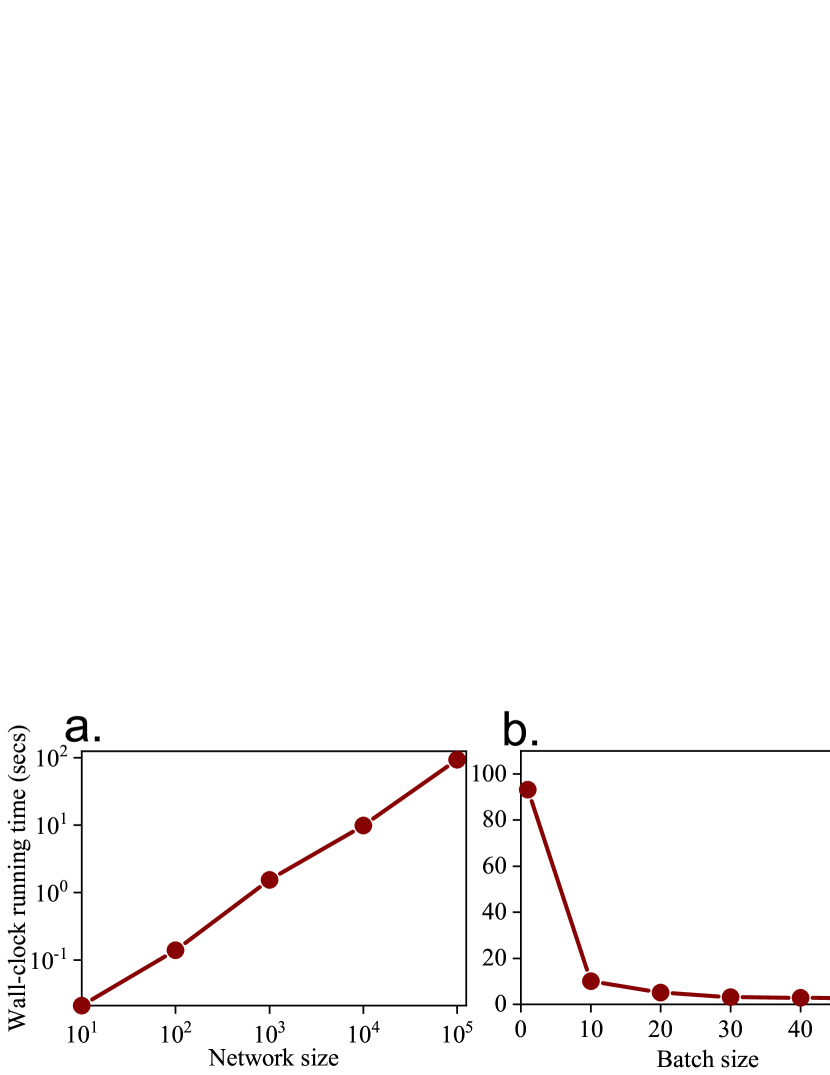
Figure 3: Wall-clock running time analysis. (a). Liner scalability of DREIM. (b). For Facebook network with budget $k=50$, the wall-clock running time decreases quickly as the batch size increases.

Table 2: Basic statistics of real-world networks. $\gamma$ denotes the exponent of the power-law degree distribution.

Network	# Nodes	# Edges	$\gamma$	Avg.Degree
Digg	29.6K	84.8K	2.79	5.72
Facebook	63.3K	816.8K	2.43	25.77
Youtube	1.13M	2.99M	2.14	5.27
LiveJournal	4.85M	69M	2.43	6.5

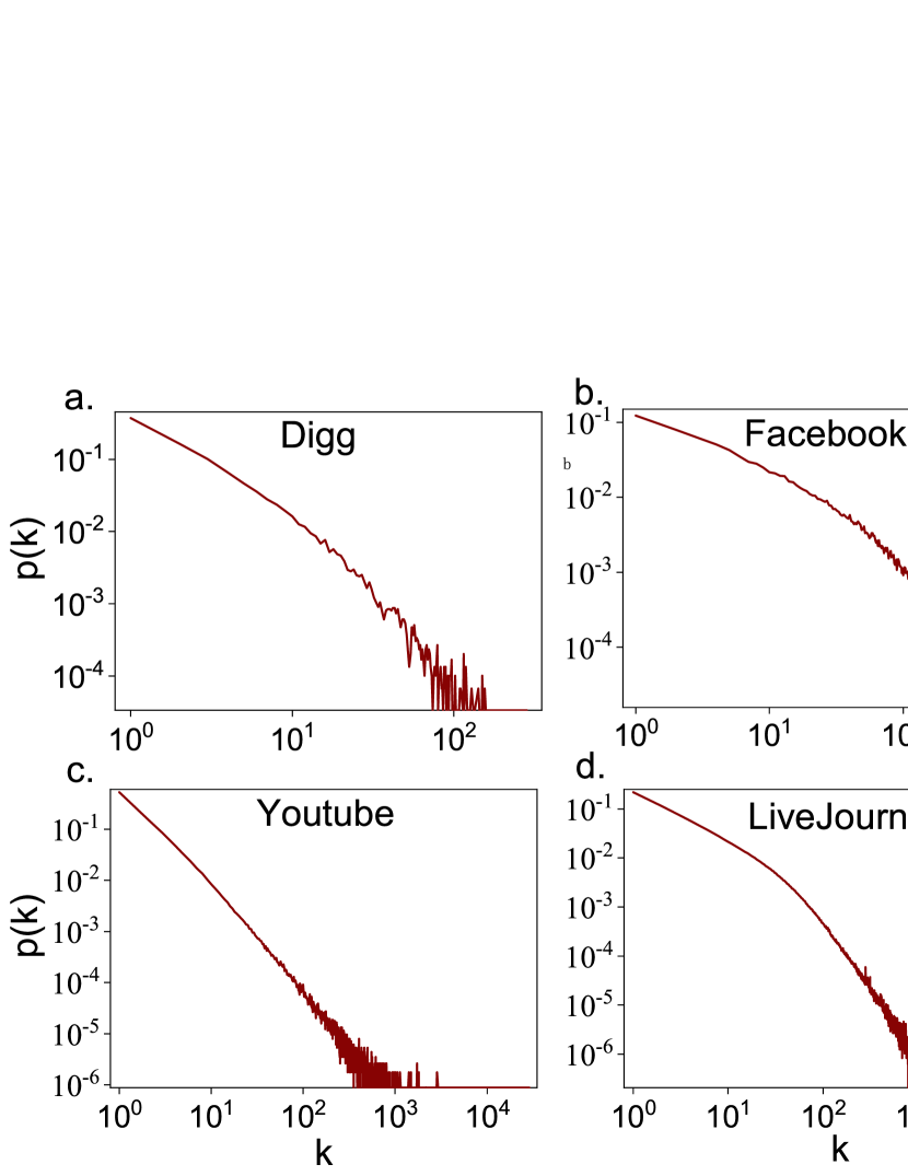
Figure 4: Degree distribution of real-world networks.

5 EXPERIMENT

We train and validate DREIMusing synthetic graphs generated by the powerlaw-cluster model as it captures two important features of the vast majority of real-world networks, i.e., small-world phenomenon [50] and power-law degree distribution [49]. And we test DREIMon both large synthetic and real-world social networks of different scales. To our best knowledge, this is the first work that considers learning for IM problem under the LT diffusion model, moreover, DREIMexceeds the spread quality of all the baselines.

5.1 Experimental setup

5.1.1 Baselines

We compare the effectiveness and efficiency of DREIMwith other baselines. IMM is the state-of-the-art approximation method according to a benchmarking study [33]. Previous work GCOMB [29] tries to solve the IM problem using reinforcement learning method and obtains similar performance to IMM. So we compare DREIMwith IMM and GCOMB. We use the code of IMM and GCOMB shared by the authors. For IMM, we set $\epsilon=0.5$ throughout the experiment as suggested by the authors. For GCOMB, to make it comparable, we change the diffusion model from IC to LT. We train and validate GCOMB on subgraphs sampled from Youtube by randomly selecting 30% of its edges, and we test GCOMB on the remaining subgraph of Youtube and the entire graphs of other networks. To reduce the randomness of the LT diffusion model, we ran 10000 diffusion processes and report the average value as the final spread.

5.1.2 Datasets

We adopt the powerlaw-cluster model to generate synthetic networks with different scales. Table 2 summarize the basic statistics of real-world networks [55] and Fig. 4 illustrates the degree distribution of them.

5.1.3 Evaluation metrics

To evaluate DREIMquantitatively, we consider the following three aspects to report DREIM’s effectiveness and efficiency.

Spread quality. We adopt the metric active rate, i.e., the proportion of active nodes to total nodes under a specific seed nodes budget $k$ to compare the spread quality with baselines.
Scalability. As analyzed before, the inference complexity of DREIMis $O(kM)$, where $k$ is the given budget and $M$ is the number of edges. We test DREIMon large networks scaling up to millions of nodes. We can see in Fig. 5 that DREIMcan effectively solve the problem of networks size up to 4.85 million.
Time complexity. We theoretically compare the time complexity of DREIMand all the baselines.

Table 3: Active rate comparison of different DREIMvariants, i.e., using distinct batch sizes on synthetic networks for $k=50$, $k=100$, $k=200$ (%). All the results are the average value for 100 networks of the same scale.

Scale	$k=50$			$k=100$			$k=200$
	DREIM-1	DREIM-10	DREIM-All	DREIM-1	DREIM-10	DREIM-All	DREIM-1	DREIM-10	DREIM-All
10000	$40.89\pm 0.42$	$\boldsymbol{41.70\pm 0.62}$	$38.72\pm 0.67$	$30.41\pm 0.32$	$\boldsymbol{34.19\pm 0.21}$	$29.62\pm 0.18$	$\boldsymbol{60.29\pm 0.21}$	$59.16\pm 0.41$	$60.20\pm 0.62$
20000	$30.41\pm 0.32$	$\boldsymbol{34.19\pm 0.21}$	$29.62\pm 0.18$	$\boldsymbol{40.59\pm 0.48}$	$38.73\pm 0.73$	$39.25\pm 0.42$	$\boldsymbol{49.98\pm 0.41}$	$49.76\pm 0.29$	$47.71\pm 0.32$
50000	$\boldsymbol{21.98\pm 0.21}$	$20.25\pm 0.56$	$21.28\pm 0.53$	$\boldsymbol{30.43\pm 0.11}$	$29.01\pm 0.65$	$28.99\pm 0.28$	$37.86\pm 0.16$	$\boldsymbol{37.94\pm 0.36}$	$36.63\pm 0.26$
100000	$\boldsymbol{17.56\pm 0.37}$	$16.76\pm 0.47$	$16.70\pm 0.37$	$\boldsymbol{23.72\pm 0.15}$	$21.03\pm 0.43$	$21.86\pm 0.68$	$\boldsymbol{29.89\pm 0.40}$	$29.39\pm 0.76$	$28.68\pm 0.47$
500000	$9.22\pm 0.68$	$9.12\pm 0.37$	$\boldsymbol{10.38\pm 0.25}$	$12.53\pm 0.18$	$\boldsymbol{12.75\pm 0.24}$	$12.57\pm 0.39$	$\boldsymbol{17.01\pm 0.34}$	$15.95\pm 0.61$	$16.46\pm 0.39$

5.2 Results on synthetic graphs

We report the active rate under different budget $k$ of DREIMand other baselines on synthetic networks scaling from 10000 to 500000 generated by the powerlaw-cluster model. Since the network generation process is stochastic, we generate 100 networks for each scale and report the mean and standard deviation. As shown in Table 1, DREIMachieves superior performance over both IMM and GCOMB in terms of active rate. One important observation is that even we train DREIMon small graphs with a scale range of $30\sim 50$, it still performs well on networks with several orders of magnitude larger scales. This is because DREIMuses the inductive graph embedding method whose parameters are independent of the network size, and for reinforcement learning, it adopts the uniform termination condition for networks with different sizes. Another observation is that the batch nodes selection strategy can bring higher solution quality. For example, as shown in Table 3, when the network scale is 10000 and 20000, DREIM-10 even obtains a higher active rate than DREIM-1. And when the network size is 500000, DREIM-All performs better than DREIM-1. This phenomenon indicates that our batch nodes selection strategy could not only decrease the time complexity, but also enhance the effectiveness of DREIM. And from Fig. 3 (a) we can also see that for budget $k=30$, the running time increases linearly with regard to the network size.

5.3 Results on real-world networks

In the last section, we see that DREIMperforms well on large synthetic graphs generated by the same model as it is trained on. In this section, we test whether DREIMcan still perform well on large real-word networks. In Fig. 5 we plot the active rate curve using different methods under different budget k for every network we test. We can see that DREIMcan always surpass all the baselines in terms of active rate for all the experiment settings, i.e., different networks and budgets. For example, when initially activating 50 nodes for Youtube, DREIMfinally activates 16.3% of the total nodes while IMM and GCOMB activate 16.1% and 15.4% of the total nodes respectively. In Fig. 3 (b), we plot the wall-clock running time curve for Facebook network with $k=50$ using different batch sizes. We can see that DREIM-10 takes 10 times less time than DREIM-1 meanwhile, as shown in Fig. 6, activates 24.5% of the total nodes, clearly higher than 23.2% and 23.0% obtained by IMM and GCOMB, meaning that the running time can be dramatically reduced by exploiting the batch nodes selection strategy and the effectiveness of DREIMis not greatly affected.

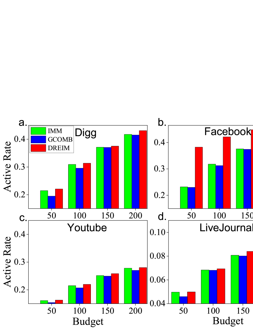
Figure 5: Active rate on real-world networks under different budget $k$.

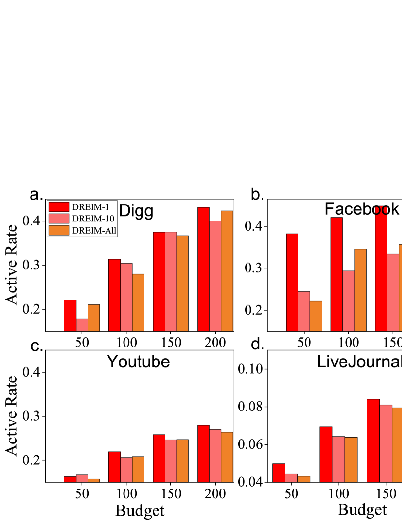
Figure 6: Active rate on real-world networks under different budget $k$ using distinct batch sizes.

5.4 Comparison of time complexity

As analyzed before, the time complexity of DREIMis $O(M+N+N\mathrm{log}N)$, for sparse real-world networks, we can say DREIMhas a linear time complexity $O(kM)$ when budget is k. And the empirical results in Fig. 3 (a) also support our theoretical analysis. For IMM, as reported by the authors, its time complexity is $O\left((k+\ell)(n+m)\log n/\varepsilon^{2}\right)$, i.e., IMM also has a near linear scalability with regard to the network size. For GCOMB, its time complexity is $O\left(|V|+\left|V^{g,K}\right|\left(dm_{G}+m_{G}^{2}\right)+\left|V^{g}\right|b\left(d+m_{Q}\right)\right)$, see [29] for details. DREIMhas a comparatively lower time complexity among all the methods. Moreover, the time complexity can be mitigated through the batch nodes selection strategy to $O(k/bM)$ supported by results in Fig. 3 (b), where $b$ is the batch size.

Table 4: Hyper-parameter values.

Hyper-parameter	Value	Description
learning rate	$1\times 10^{-4}$	the learning rate used by Adam optimizer
embedding dimension	64	dimension of node embedding vector
maximum episodes	$1\times 10^{6}$	maximum episodes for the training process
layer iterations	3	number of message-passing iterations
reconstruction loss weight	$1\times 10^{-3}$	weight of graph reconstruction loss

5.5 Other settings

All experiments are performed on a 32-core sever with 64GB memory. We conduct the validation process every 300 iterations and conduct the play game process every 10 iterations. For the $n$-step $Q$-learning, we set $n=5$ and 64 experiences are sampled uniformly random from the experience replay buffer. We implement the model using Tensorflow and use the Adam optimizer, and the hyper-parameters are summarized in Table 4.

To reduce the randomness of the diffusion process, we run a large number (e.g., 10000) of diffusion process and use the average value as the final spread value.

6 DISCUSSION

In this section, we try to interpret what heuristics DREIMhas learned. We further discuss the effect of different termination conditions on DREIM’s performance.

6.1 Policy analysis of DREIM

In this section, we try to interpret DREIM’s success through two observations. Firstly, the agent learns to minimize the Return. To make it clear, we draw the inactive rate curve, as shown in Fig. 2 (a), where the Return can be approximately computed by the area under the curve. Note that minimizing the Return guides the agent to become more and more intelligent in two folds. One is that it tries to select seed nodes as few as possible to activate all the nodes, and the other one is that it prefers to select nodes that bring more decrease on inactive rate at each step. These two aspects coordinate together to guide the agent to find better influencers. Secondly, in terms of the seed nodes, DREIMtends to find the influencers which have a balance of connectivity based centrality, e.g., degree centrality and distance based centrality, e.g. betweenness centrality.

6.2 Different termination conditions

In what follows, we discuss the influences of using different termination conditions of the interaction process for training and inference.

During the training phase, the interaction process ends when all nodes are activated, which is a uniform state for networks of different scales while during the inference phase, we use the batch nodes selection strategy, and terminates when $|{\mathcal{S}}|=k$, where $k$ is the budget. Previous works like [29, 53] adopt $|{\mathcal{S}}|=k$ as the termination condition for both training and inference. We argue this setting will restrict DREIM’s generalization ability because the termination state can be very different for networks of different scales. One concern is that, using different termination condition seems to be unreasonable, since traditionally researchers usually apply their model to similar problem instances. However, the empirical results in Table 1 and Fig. 5 do show that though we use different termination conditions for training and inference, we still obtain better spread quality for all budgets. We will leave exploring explanations for this phenomenon as a future direction.

7 CONCLUSION

In this paper, we formalize the influence maximization problem as a Markov decision process, and we design a novel reinforcement learning framework DREIMto tackle this problem. To our best knowledge, DREIMis the first work that obtains significant superior spread quality over traditional state-of-the-art method IMM. We combine the graph neural network and deep reinforcement learning together. We treat the embedding of the virtual node and the embeddings of real nodes as the state and action of the reinforcement learning. By exploiting a batch nodes selection strategy, the computational time is greatly reduced without compromising much on solution quality.

We use synthetic graphs generated by the powerlaw-cluster model to train DREIMand test DREIMon several large synthetic and real-world social networks of different sizes from thousands to millions. And the empirical results show that DREIMhas exceeded the performance of all the baselines.

For future work, one possible direction is to seek theoretical guarantees. Another important direction is to design more powerful and interpretable graph representation learning methods to better preserve graph information.

FUNDING

This work was supported in part by the National Natural Science Foundation of China (Nos. 61803248, 61872093, and U20B2051), the National Key R & D Program of China (No. 2018YFB1305104), Shanghai Municipal Science and Technology Major Project (Nos. 2018SHZDZX01 and 2021SHZDZX03), ZJ Lab, and Shanghai Center for Brain Science and Brain-Inspired Technology.

DATA AVAILABILITY STATEMENT

The data underlying this article are available in SNAP, at http://snap.stanford.edu/data.

References

- [1] Nguyen, H. T., Thai, M. T., and Dinh, T. N. (2016) Stop-and-stare: Optimal sampling algorithms for viral marketing in billion-scale networks. Proceedings of the International Conference on Management of Data, San Francisco, California, 26 June-01 July, pp. 695–710. ACM, New York.
- [2] Chen, W., Wang, C., and Wang, Y. (2010) Scalable influence maximization for prevalent viral marketing in large-scale social networks. Proceedings of the 16th International Conference on Knowledge Discovery and Data Mining, Washington, D.C., 25-28 July, pp. 1029–1038. ACM, New York.
- [3] Kempe, D., Kleinberg, J., and Tardos, E. (2003) Maximizing the spread of influence through a social network. Proceedings of the 9th International Conference on Knowledge Discovery and Data Mining, Washington, D.C., 24-27 August, pp. 137–146. ACM, New York.
- [4] Tang, J., Tang, X., Xiao, X., and Yuan, J. (2018) Online processing algorithms for influence maximization. Proceedings of the International Conference on Management of Data, Houston, TX, USA, 10-15 June, pp. 991–1005. ACM, New York.
- [5] Chen, W., Yuan, Y., and Zhang, L. (2010) Scalable influence maximization in social networks under the linear threshold model. Proceedings of the International Conference on Data Mining, Sydney, Australia, 14-17 December, pp. 88–97. IEEE.
- [6] Cheng, S., Shen, H., Huang, J., Zhang, G., and Cheng, X. (2013) Staticgreedy: solving the scalability-accuracy dilemma in influence maximization. Proceedings of the 22nd International Conference on Information and Knowledge Management, San Francisco, California, 27 October-1 November, pp. 509–518. ACM, New York.
- [7] Cheng, S., Shen, H., Huang, J., Chen, W., and Cheng, X. (2014) Imrank: Influence maximization via finding self-consistent ranking. Proceedings of the 37th International Conference on Research Development in Information Retrieval, Gold Coast, Queensland, 06-11 July, pp. 475–484. ACM, New York.
- [8] Cohen, E., Delling, D., Pajor, T., and Werneck, R. F. (2014) Sketch-based influence maximization and computation: Scaling up with guarantees. Proceedings of the 23rd International Conference on Information and Knowledge Management, Shanghai, China, 3-7 November, pp. 629–638. ACM, New York.
- [9] Galhotra, S., Arora, A., Virinchi, S., and Roy, S. (2015) Asim: A scalable algorithm for influence maximization under the independent cascade model. Proceedings of the 24th International Conference on World Wide Web, Florence, Italy, 18-22 May, pp. 35–36. ACM, New York.
- [10] Galhotra, S., Arora, A., and Roy, S. (2016) Holistic influence maximization: Combining scalability and efficiency with opinion-aware models. Proceedings of the International Conference on Management of Data, San Francisco, California, 26 June-01 July, pp. 743–758. ACM, New York.
- [11] Goyal, A., Lu, W., and Lakshmanan, L. V. (2011) Simpath: An efficient algorithm for influence maximization under the linear threshold model. Proceedings of the International Conference on Data Mining, Vancouver, BC, Canada, 11-14 December, pp. 211–220. IEEE.
- [12] Goyal, A., Bonchi, F., and Lakshmanan, L. V. S. (2011) A data-based approach to social influence maximization. Proc. VLDB Endow., 5, 73–84.
- [13] Jung, K., Heo, W., and Chen, W. (2012) Irie: Scalable and robust influence maximization in social networks. Proceedings of the International Conference on Data Mining, Brussels, Belgium, 10-13 December, pp. 918–923. IEEE.
- [14] Lee, J.-R. and Chung, C.-W. (2014) A fast approximation for influence maximization in large social networks. Proceedings of the 23rd International Conference on World Wide Web, Seoul, Korea, 7-11 April, pp. 1157–1162. ACM, New York.
- [15] Ohsaka, N., Akiba, T., Yoshida, Y., and Kawarabayashi, K.-I. (2014) Fast and accurate influence maximization on large networks with pruned monte-carlo simulations. Proceedings of the 28th AAAI Conference on Artificial Intelligence, Québec City, Québec, Canada, 27-31 July, pp. 138–144. AAAI Press.
- [16] Song, G., Zhou, X., Wang, Y., and Xie, K. (2015) Influence maximization on large-scale mobile social network: A divide-and-conquer method. IEEE Trans. Parallel Distrib. Syst., 26, 1379–1392.
- [17] Tang, J., Tang, X., and Yuan, J. (2017) Influence maximization meets efficiency and effectiveness: A hop-based approach. Proceedings of the International Conference on Advances in Social Networks Analysis and Mining, Sydney, Australia, 31 July-03 August, pp. 64–71. ACM, New York.
- [18] Zhou, C., Zhang, P., Guo, J., Zhu, X., and Guo, L. (2013) Ublf: An upper bound based approach to discover influential nodes in social networks. Proceedings of the International Conference on Data Mining, Dallas, TX, USA, 7-10 December, pp. 907–916. IEEE.
- [19] Zhou, C., Zhang, P., Guo, J., and Guo, L. (2014) An upper bound based greedy algorithm for mining top-k influential nodes in social networks. Proceedings of the 23rd International Conference on World Wide Web, Seoul, Korea, 7-11 April, pp. 421–422. ACM, New York.
- [20] Leskovec, J., Krause, A., Guestrin, C., Faloutsos, C., VanBriesen, J., and Glance, N. (2007) Cost-effective outbreak detection in networks. Proceedings of the 13th International Conference on Knowledge Discovery and Data Mining, San Jose, California, 12-15 August, pp. 420–429. ACM, New York.
- [21] Borgs, C., Brautbar, M., Chayes, J. T., and Lucier, B. (2014) Maximizing social influence in nearly optimal time. In Chekuri, C. (ed.), Proceedings of the 25th Annual ACM-SIAM Symposium on Discrete Algorithms, Portland, Oregon, 5-7 January, pp. 946–957. SIAM.
- [22] Tang, Y., Xiao, X., and Shi, Y. (2014) Influence maximization: Near-optimal time complexity meets practical efficiency. Proceedings of the International Conference on Management of Data, Snowbird, Utah, USA, 22-27 June, pp. 75–86. ACM, New York.
- [23] Tang, Y., Shi, Y., and Xiao, X. (2015) Influence maximization in near-linear time: A martingale approach. Proceedings of the International Conference on Management of Data, Melbourne, Victoria, Australia, 31 May-04 June, pp. 1539–1554. ACM, New York.
- [24] Bucur, D. and Iacca, G. (2016) Influence maximization in social networks with genetic algorithms. In Squillero, G. and Burelli, P. (eds.), Applications of Evolutionary Computation, Cham, 30 March-1 April, pp. 379–392. Springer International Publishing.
- [25] Tabak, B. M., Takami, M., Rocha, J. M., Cajueiro, D. O., and Souza, S. R. (2014) Directed clustering coefficient as a measure of systemic risk in complex banking networks. Physica A, 394, 211–216.
- [26] Wilson, C., Boe, B., Sala, A., Puttaswamy, K. P., and Zhao, B. Y. (2009) User interactions in social networks and their implications. Proceedings of the 4th European Conference on Computer Systems, Nuremberg, Germany, 1-3 April, pp. 205–218. ACM, New York.
- [27] Chen, W., Wang, Y., and Yang, S. (2009) Efficient influence maximization in social networks. Proceedings of the 15th International Conference on Knowledge Discovery and Data Mining, Paris, France, 28 June-1 July, pp. 199–208. ACM, New York.
- [28] Dai, H., Khalil, E. B., Zhang, Y., Dilkina, B., and Song, L. (2017) Learning combinatorial optimization algorithms over graphs. Proceedings of the 31st International Conference on Neural Information Processing Systems, Long Beach, California, 4-9 December, pp. 6351–6361. Curran Associates Inc., Red Hook, NY, USA.
- [29] Manchanda, S., MITTAL, A., Dhawan, A., Medya, S., Ranu, S., and Singh, A. (2020) Gcomb: Learning budget-constrained combinatorial algorithms over billion-sized graphs. Proceedings of the 34th International Conference on Neural Information Processing Systems, Online Event, 6-12 December, pp. 20000–20011. Curran Associates, Inc., Red Hook, NY, USA.
- [30] Li, Z., Chen, Q., and Koltun, V. (2018) Combinatorial optimization with graph convolutional networks and guided tree search. Proceedings of the 32nd International Conference on Neural Information Processing Systems, Montréal, Canada, 3-8 December, pp. 537–546. Curran Associates Inc., Red Hook, NY, USA.
- [31] Richardson, M. and Domingos, P. (2002) Mining knowledge-sharing sites for viral marketing. Proceedings of the 8th International Conference on Knowledge Discovery and Data Mining, Edmonton, Alberta, Canada, 23-26 July, pp. 61–70. ACM, New York.
- [32] Domingos, P. and Richardson, M. (2001) Mining the network value of customers. Proceedings of the International 7th Conference on Knowledge Discovery and Data Mining, San Francisco, California, 26-29 August, pp. 57–66. ACM, New York.
- [33] Arora, A., Galhotra, S., and Ranu, S. (2017) Debunking the myths of influence maximization: An in-depth benchmarking study. Proceedings of the International Conference on Management of Data, Chicago, Illinois, USA, 14-19 May, pp. 651–666. ACM, New York.
- [34] Sen, P., Namata, G., Bilgic, M., Getoor, L., Galligher, B., and Eliassi-Rad, T. (2008) Collective classification in network data. AI Mag., 29, 93.
- [35] Liben-Nowell, D. and Kleinberg, J. (2003) The link prediction problem for social networks. Proceedings of the 12th International Conference on Information and Knowledge Management, New York, NY, 2-8 November, pp. 556–559. ACM, New York.
- [36] Herman, I., Melançon, G., and Marshall, M. S. (2000) Graph visualization and navigation in information visualization: A survey. IEEE Trans. Vis. Comput. Graph., 6, 24–43.
- [37] Fan, C., Zeng, L., Ding, Y., Chen, M., Sun, Y., and Liu, Z. (2019) Learning to identify high betweenness centrality nodes from scratch: A novel graph neural network approach. Proceedings of the 28th International Conference on Information and Knowledge Management, Beijing, China, 3-7 November, pp. 559–568. ACM, New York.
- [38] Kipf, T. N. and Welling, M. (2017) Semi-supervised classification with graph convolutional networks. Proceedings of the 5th International Conference on Learning Representations, Toulon, France, 24-26 April. OpenReview.net.
- [39] Hamilton, W. L., Ying, R., and Leskovec, J. (2017) Inductive representation learning on large graphs. Proceedings of the 31st International Conference on Neural Information Processing Systems, Long Beach, California, 4-9 December, pp. 1025–1035. Curran Associates Inc., Red Hook, NY, USA.
- [40] Sutton, R. S. and Barto, A. G. (2018) Reinforcement learning: An introduction. MIT press.
- [41] Bengio, Y., Lodi, A., and Prouvost, A. (2021) Machine learning for combinatorial optimization: A methodological tour d’horizon. Eur. J. Oper. Res., 290, 405–421.
- [42] Bello, I., Pham, H., Le, Q. V., Norouzi, M., and Bengio, S. (2016) Neural combinatorial optimization with reinforcement learning. CoRR, abs/1611.09940.
- [43] Selsam, D., Lamm, M., Bünz, B., Liang, P., de Moura, L., and Dill, D. L. (2019) Learning a SAT solver from single-bit supervision. Proceedings of the 7th International Conference on Learning Representations, New Orleans, LA, USA, 6-9 May. OpenReview.net.
- [44] Bonami, P., Lodi, A., and Zarpellon, G. (2018) Learning a classification of mixed-integer quadratic programming problems. In van Hoeve, W.-J. (ed.), Integration of Constraint Programming, Artificial Intelligence, and Operations Research, Delft, The Netherlands, 26-29 June, pp. 595–604. Springer International Publishing.
- [45] Wilder, B., Dilkina, B., and Tambe, M. (2019) Melding the data-decisions pipeline: Decision-focused learning for combinatorial optimization. Proceedings of the 23rd AAAI Conference on Artificial Intelligence, Honolulu, Hawaii, USA, 27 January-1 February, pp. 1658–1665. AAAI Press.
- [46] Lodi, A. and Zarpellon, G. (2017) On learning and branching: a survey. TOP, 25, 207–236.
- [47] Cappart, Q., Goutierre, E., Bergman, D., and Rousseau, L.-M. (2019) Improving optimization bounds using machine learning: Decision diagrams meet deep reinforcement learning. Proceedings of the 23rd AAAI Conference on Artificial Intelligence, Honolulu, Hawaii, USA, 27 January-1 February, pp. 1443–1451. AAAI Press.
- [48] Fan, C., Zeng, L., Sun, Y., and Liu, Y.-Y. (2020) Finding key players in complex networks through deep reinforcement learning. Nat. Mach. Intell., 2, 317–324.
- [49] Barabási, A.-L. and Albert, R. (1999) Emergence of scaling in random networks. Science, 286, 509–512.
- [50] Watts, D. J. and Strogatz, S. H. (1998) Collective dynamics of ‘small-world’ networks. Nature, 393, 440–442.
- [51] Erdös, P. and Rényi, A. (1959) On random graphs i. Publ. Math.-Debr., 6, 290.
- [52] Holme, P. and Kim, B. J. (2002) Growing scale-free networks with tunable clustering. Phys. Rev. E, 65, 026107.
- [53] Sun, Y., Wang, S., Tang, X., Hsieh, T.-Y., and Honavar, V. (2020) Adversarial attacks on graph neural networks via node injections: A hierarchical reinforcement learning approach. Proceedings of The Web Conference, Taipei, Taiwan, 20-24 April, pp. 673–683. ACM, New York.
- [54] Riedmiller, M. (2005) Neural fitted q iteration – first experiences with a data efficient neural reinforcement learning method. In Gama, J., Camacho, R., Brazdil, P. B., Jorge, A. M., and Torgo, L. (eds.), Machine Learning: ECML, Porto, Portugal, 3-7 October, pp. 317–328. Springer Berlin Heidelberg.
- [55] Leskovec, J. and Krevl, A. (2014). SNAP Datasets: Stanford large network dataset collection. http://snap.stanford.edu/data.