Self-Supervised Blind Source Separation via Multi-Encoder Autoencoders

Abstract

The task of blind source separation (BSS) involves separating sources from a mixture without prior knowledge of the sources or the mixing system. This is a challenging problem that often requires making restrictive assumptions about both the mixing system and the sources. In this paper, we propose a novel method for addressing BSS of non-linear mixtures by leveraging the natural feature subspace specialization ability of multi-encoder autoencoders with fully self-supervised learning without strong priors. During the training phase, our method unmixes the input into the separate encoding spaces of the multi-encoder network and then remixes these representations within the decoder for a reconstruction of the input. Then to perform source inference, we introduce a novel encoding masking technique whereby masking out all but one of the encodings enables the decoder to estimate a source signal. To this end, we also introduce a so-called pathway separation loss that encourages sparsity between the unmixed encoding spaces throughout the decoder’s layers and a so-called zero reconstruction loss on the decoder for coherent source estimations. In order to carefully evaluate our method, we conduct experiments on a toy dataset and with real-world biosignal recordings from a polysomnography sleep study for extracting respiration.

1 Introduction

Source separation is the process of separating a mixture of sources into their unmixed source components. Blind source separation (BSS) aims to perform source separation without any prior knowledge of the sources or the mixing process and is widely applied in various fields such as biomedical engineering, audio processing, image processing, and telecommunications. Classical approaches to blind source separation such as those incorporating independent component analysis (ICA) [14, 16, 15, 2], principal component analysis (PCA) [20] or non-negative matrix factorization (NMF) [23, 41] are effective at separating sources only under specific conditions. For example, these approaches make assumptions such as statistical independence or linear dependency between sources, which limits their potential applications and effectiveness [21].

Blind source separation has a long-standing shared connection with deep learning as they both originally take inspiration from biological neural networks [23, 15, 3]. The connection between these two fields exists since even before the advancement of modern deep learning approaches. Of course, with the explosive rise of deep learning, recent approaches to source separation often incorporate deep neural architectures employing supervised learning, semi-supervised learning, or transfer learning [19, 42, 18]. Further, in deep neural network architectures such as transformers with multi-headed attention [51], or the pivotal AlexNet model [22], originally trained with two sparsely connected convolutional encoders, the tendency for separated encoding structures that share the same inputs to specialize in feature subspaces has been observed. Several works have shown feature subspace specialization to be a crucial aspect of the learning process in the case of transformers [53, 52, 46]. Generally, the previous work focuses primarily on the interpretability of the representations that arise from this phenomenon of feature subspace specialization.

Artificial neural networks are proven to be a successful approach for many source separation tasks in the literature [40, 39, 43, 7, 44, 5, 35, 57, 26, 9, 58]. In this paper, we utilize the natural feature subspace specialization of neural networks with multiple encoder-like structures for BSS. Our proposed method employs a fully self-supervised training process such that the network is given no examples of the sources or information about the feature distribution of the sources, and therefore, is fully compatible with the problem statement of BSS in which we do not have any prior knowledge of the sources or the mixing process and only have access to the mixture for separation. Our proposed method utilizes a convolutional multi-encoder-single-decoder autoencoder that learns to separate the feature subspaces of the given mixture’s sources within the encoding space of the network. The network decoder learns to remix the concatenated outputs of the multiple encoders to predict the original input mixture. This is achieved with a simple reconstruction loss between the network’s input and output without making any strong assumptions about the source signals or the mixing process. Significantly, no assumption of linear separability from the mixture is made for the sources; an assumption that many other works incorporate as a key component of the loss design. In addition, we propose two key regularization methods for enabling source estimation: the pathway separation loss and the zero reconstruction loss. The pathway separation loss aims to keep the weight connections shared by source encoding spaces and subsequent mappings sparse throughout the decoder by decaying the submatrices in the weights that connect separate encoding spaces toward zero. In other words, we encourage learned pathways in the weights of the decoder that each decode a specific encoding space such that all of the pathways are sparsely connected. The degree of sparseness can be controlled by a hyperparameter which scales the contribution of the loss term with respect to the total loss. After training, source estimations are produced using a novel encoding masking technique where all but a single encoding are masked with zero arrays and then the resulting output of the decoder is the source estimation associated with the active encoding i.e. the encoding that is not masked. The quality of source estimations is ensured by applying the zero reconstruction loss on the decoder during the training phase. The zero reconstruction loss reduces the impact that parameters unrelated to the target source have on the decoding of the active encoding space for source estimations by having the decoder construct a zero output when given an all-zero encoding.

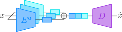
(a) Blind source separation training procedure.

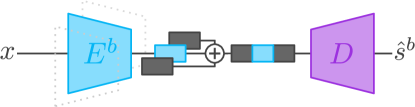
(b) Blind source separation inference procedure.

Figure 1: Illustration of the general training and inference procedure for the proposed method.

To the best of our knowledge, our proposed method is the first in the literature to employ fully self-supervised multi-encoder autoencoders for performing BSS with a special focus on non-linearly mixed sources. The effectiveness of the proposed method is evaluated on a toy dataset of non-linear mixtures, and on raw real-world electrocardiogram (ECG) and photoplethysmogram (PPG) signals for extracting respiratory signals. The results demonstrate that (a) the encoders of the multi-encoder autoencoder trained with our method can effectively discover and separate the sources of the proposed toy dataset, consisting of non-linearly mixed triangle and circle shapes, and (b) our method can be successfully applied to estimate a respiratory signal from ECG and PPG signals in a fully self-supervised manner where it shows comparable results with existing methods.

We summarize our contributions in this paper as follows:

• We propose a novel method for BSS by employing fully self-supervised multi-encoder autoencoders for the first time in the literature.

• We propose a novel encoding masking technique for source separation inference, and two novel model regularization techniques, the pathway separation loss and the zero reconstruction loss for implicit source separation learning and source estimation.

• We demonstrate the ability of the proposed method to extract meaningful respiratory signals from raw ECG and PPG recordings using a fully self-supervised learning scheme.

2 Related Work

In the audio domain, source separation is applied to various fields; for example, in speech separation where the voices of different individuals are the source signals, and also in music source separation, where the individual instruments that comprise the mixed audio are the target sources. In the literature, different methods for source separation based on deep learning algorithms have been proposed. Wave-U-Net [43] brings end-to-end source separation using time-domain waveforms. The deep attractor network (DANet), [7] uses an LSTM network to map mixtures in the time-frequency domain into an embedding space which is then used with so-called attractors, taking inspiration from cognitive speech perception theories in neuroscience, to create masks for each source.

Generating masks on a per-source basis makes the assumption that the source is linearly separable from the mixture which is a reasonable and often necessary assumption to make for many problems. Deep clustering [10] starts by embedding time-frequency representations of a mixed audio signal, then using K-means clustering to segment multiple sources, and lastly with the informed segmentation uses sparse non-negative matrix factorization to perform source separation. TaSNet [28] uses a three-stage network with an encoder that estimates a mixture weight, a separation module that estimates source masks, and a decoder for reconstructing source signals. Other works make extensions to TaSNet such as the dual-path RNN [27] that improves performance while reducing the model size, Conv-TasNet [29] which brings a fully convolutional approach to the prior method, or Meta-TaSNet [38] which introduces meta-learning to generate the weights for source extraction models. As is the current trend in deep learning research, transformer models also show an impressive capability for audio source separation due to their explicit design for sequence modeling [44, 5, 35, 57].

Deep learning approaches to separating superimposed images, shadow and shading separation, or reflection separation are areas of active research within the domain of computer vision. One work [13] approaches the task of separating superimposed handwritten digits from the MNIST dataset and superimposed images of handbags and shoes by learning a single mask to separate two sources. For the first source, the mixed signal is multiplied by the mask, and for the second source, the mixed signal is multiplied by one minus the mask, which inverts the values of the mask. In another work, [32] a self-supervised BSS approach based on variational autoencoders makes the assumption that the summation of the extracted sources is equal to the mixed signal. The authors have demonstrated the effectiveness of the approach for separating linearly mixed handwritten digits and for separating mixed audio spectrograms where two sources are assumed to be the summation of the given mixture. Liu Y et al. [26] use a dual encoder-generator architecture with a cycle consistency loss to separate linear mixtures, more specifically the addition of two sources, using self-supervision. They explore the tasks of separating backgrounds and reflections, and separating albedo and shading. The Double-DIP method [9] seeks to solve image segmentation, image haze separation, and superimposed image separation with coupled deep-image-prior networks to predict a mask for separating two image layers. Separation techniques that use a single mask to separate two sources make the assumption that there is a solution that can linearly separate a sample of mixed sources even though the process of generating said mask may be non-linear. Zou Z et al. [58] propose their own method for separating superimposed images which uses a decomposition encoder with additional supervision from a separation critic and a discriminator to improve the quality of the source estimations.

Other domains where deep learning approaches to source separation are in use include biosignals processing tasks [40, 39, 24, 33, 1], finance [40], and communication signals processing [56]. There are many challenges surrounding source separation and BSS tasks, but data-driven solutions, such as deep learning, are shown to be an effective strategy for solving these problems.

3 Proposed method

3.1 Preliminaries

Multi-Encoder Autoencoders

Autoencoders are a class of self-supervised neural networks that compress high-dimensional data into a low-dimensional latent space $z$ using an encoder network $E_{\theta}$, parameterized by $\theta$, and then reconstruct the input data from the latent space using a decoder network $D_{\phi}$, parameterized by $\phi$. During the training process, the encoder must learn to preserve the most salient information of the original data in order to make accurate reconstructions [11].

$$z=E_{\theta}(x),\ \hat{x}=D_{\phi}(z)$$ (1)

$$\min_{\theta,\phi}\mathcal{L}_{\text{recon.}}(x,D_{\phi}(E_{\theta}(x)))$$ (2)

Multi-encoder autoencoders [47] use a total of $N$ encoders $\bm{E_{\theta}}=\left[E^{0}_{\theta_{0}}\ E^{1}_{\theta_{1}}\ \ldots\ E^{N}_{\theta_{N}}\right]$, which all take the same input $x$ for this paper, unlike prior works, such that their separate encodings $\bm{z}=\left[z_{0}\ \ldots\ z_{N}\right]$ are combined in some manner before being passed into the decoder $D_{\phi}$ for reconstruction.

$$\bm{z}=\bm{E_{\theta}}(x)=\left[E^{0}_{\theta_{0}}(x)\ E^{1}_{\theta_{1}}(x)\ \ldots\ E^{N}_{\theta_{N}}(x)\right],\ \hat{x}=D_{\phi}(\bm{z})$$ (3)

$$\min_{\bm{\theta},\phi}\mathcal{L}_{recon.}(x,D_{\phi}(\bm{E_{\theta}}(x)))$$ (4)

Blind Source Separation

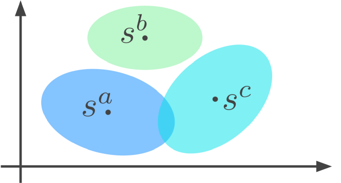
(a)

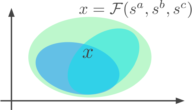
(b)

Figure 2: Illustration showing the mixing of source feature subspaces by a mixing system $\mathcal{F}$.

A formal definition of blind source separation is given as follows: For some set of $N$ source signals $\bm{s}(t)$ and some set of $K$ noise signals $\bm{n}(t)$, a mixing system $\mathcal{F}$ operates on $\bm{s}(t)$ and $\bm{n}(t)$ to produce a mixed signal $x(t)$. Further, the mixing system $\mathcal{F}$ may be non-linear and non-stationary in time or space $t$.

$$\bm{s}(t)=\left[s_{0}(t)\ s_{1}(t)\ \ldots\ s_{N}(t)\right]$$ (5)

$$\bm{n}(t)=\left[n_{0}(t)\ n_{1}(t)\ \ldots\ n_{K}(t)\right]$$ (6)

$$x(t)=\mathcal{F}(\bm{s}(t),\bm{n}(t),t)$$ (7)

In BSS, the goal is either to find an inverse mapping of the mixing system $\mathcal{F}^{-1}$ or extract the source signals $\bm{s}(t)$ given only the mixture $x$. Since the mixing system $\mathcal{F}$ is often non-linear and time-variant for many real-world problems, the problem of BSS is especially challenging due to the additional ambiguity it creates in the mapped feature space as illustrated in Figure 2. 2(a) shows a graph with three well-separated feature subspaces, $s^{a}$, $s^{b}$, and $s^{c}$, that correspond to the sources in some set of mixtures. 2(b) shows a graph where the mixing system $\mathcal{F}$ maps the source feature subspaces into a new feature space where there may be increased ambiguity between the source feature subspaces or in the worst case complete ambiguity.

3.2 Blind Source Separation with Multi-Encoder Autoencoders

In this paper, we train a multi-encoder autoencoder for reconstructing input mixtures where the encoders specialize in the feature subspaces of different sources as an emergent property. Specifically, the encoders unmix the sources within the encoding space of the network, and the decoder remixes the sources such that each source component removed in the encoding space results in the source being removed from the output reconstruction. In 1(a), the training phase is shown during which all encoders $\bm{E}$ are active and the expected output of the network is a reconstruction $\hat{x}$ of the input signal $x$. However during inference, shown in 1(b), only one encoder is active and the expected output is the source signal $s^{n}$ that corresponds to the source feature subspace that the active encoder $E^{n}$ specializes in. In place of the encodings from non-active encoders, zero matrices of the same size are concatenated to the active encoder’s output encoding, keeping the position of the active encoding in place.

Multi-Encoder Design and Regularization

As stated in the description of multi-encoder autoencoders (i.e., subsection 3.1), $N$ encoders $\bm{E_{\theta}}=\left[E^{0}_{\theta_{0}}\ E^{1}_{\theta_{1}}\ \ldots\ E^{N}_{\theta_{N}}\right]$, parameterized by $\bm{\theta}=\left[\theta_{0}\ \theta_{1}\ \ldots\ \theta_{N}\right]$, are chosen and produce encodings $\bm{z}=\left[z^{0}\ z^{1}\ \ldots\ z^{N}\right]$ for input variables $x\in\mathbb{R}^{C\times M}$ where $M$ represents an arbitrary number of dimensions. Prior knowledge of the number of sources is not strictly necessary for choosing the number of encoders as overestimating can result in dead encoders that have no contribution to the final source reconstruction though they may still contribute information about the mixing system. An occurrence of such dead encoders is exemplified later in subsection 4.1.

Batch normalization [17] is applied to all layers with the exception of the output of each encoder. We apply an L2 regularization loss (8) to the output of each encoder during training as follows to prevent these values from growing too large and causing exploding gradients, a role that batch normalization fills for the hidden layers of each encoder.

$$\mathcal{L}_{\text{z}}=\lambda_{\bm{z}}\frac{1}{Nh}\sum_{z^{n}\in\bm{z}}\|z^{n}\|_{2}^{2}$$ (8)

where $\|z^{n}\|_{2}^{2}$ represents the Euclidean norm of some encoding $z^{n}$ squared, the coefficient $\lambda_{\bm{z}}$ controls the penalty strength, and $h$ represents the size of the encoding (product of the channel size and spatial size).

$$Z=E^{0}(x)\oplus E^{1}(x)\oplus\ldots\oplus E^{N}(x)$$ (9)

where the $\oplus$ operator represents concatenation along the appropriate dimension. As the final step of the encoding phase, the encodings $\bm{z}$ are concatenated either along the channel dimension for fully convolutional networks or along the width dimension for linear encodings to produce the input for the decoder $Z$. One final important consideration for designing the encoders is choosing a proper encoding size. The size should not be so small as to prevent good reconstructions but also not so large that every encoder generalizes to the entire feature space rather than specializing.

Decoder Design and Regularization

The proposed method uses a standard single decoder architecture $D_{\phi}$ parameterized by $\phi$, as described previously in subsection 3.1, with input $Z$ such that the reconstruction $\hat{x}=D_{\phi}(Z)$. In this paper, two novel regularization techniques are designed for guiding the network toward conducting blind source separation. Other considerations include the use of weight normalization on the output layer and the use of group normalization.

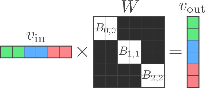
(a)

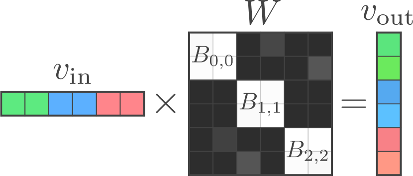
(b)

Figure 3: Illustration of the effect that the pathway separation loss has on weight matrices while decoding separate encoding spaces.

A so-called pathway separation loss is proposed for each layer in the decoder, with the exception of the output layer, to encourage sparse mixing of the encodings and their mappings throughout the decoder. Each pathway consists of a subset of corresponding submatrices in each layer that are not only responsible for decoding their respective source encodings but also control how much information from other encoding spaces is allowed to be mixed. The result is source encodings are allowed to flow through the decoder with varying degrees of influence from other encoding spaces. For a given layer the weights are first segmented into a set of blocks or non-overlapping submatrices $\bm{B}$ where the number of blocks is equal to the number of encoders squared i.e. $N^{2}$. For each block $B_{i,j}$ in the weight $W$, with elements $w\in W$, the height and width are equal to the input size $C_{\text{in}}$ and the output size $C_{\text{out}}$ of $W$ divided by the number of encoders $N$. For convolutional layers, this process is generalized with respect to the channel dimensions. Then all submatrices $B_{i,j}$ in the set of submatrices $\bm{B}$, where $i\neq j$ i.e. off-diagonal blocks, are decayed towards zero using the L1 norm leading to a partial or full separation of the encoding spaces in the decoder. This is to say that blocks on the diagonal are responsible for decoding specific encodings and the blocks not on the diagonal are responsible for the remixing of encoding spaces. The impacts of the pathway separation loss for a fully connected layer are illustrated in Figure 3. In the case that all off-diagonal weights are exactly zero 3(a), there is no mixing across the encoding spaces shown. However, if the off-diagonal blocks are exactly zero for all layers in the decoder this is a hard assumption of linear separability. To make a soft assumption of linear separability, the off-diagonal blocks are rather decayed towards zero giving the network the option to use the mixing weights when necessary as shown in 3(b).

$$W=\bm{B}=\begin{bmatrix}B_{0,0}&B_{0,1}&\cdots&B_{0,N}\\ B_{1,0}&B_{1,1}&\cdots&B_{1,N}\\ \vdots&\vdots&\ddots&\vdots\\ B_{N,0}&B_{N,1}&\cdots&B_{N,N}\\ \end{bmatrix},\ B_{i,j}=\begin{bmatrix}w_{\frac{C_{\text{in}}}{N}i,\frac{C_{\text{out}}}{N}j}&\cdots&w_{\frac{C_{\text{in}}}{N}i,\frac{C_{\text{out}}}{N}(j+1)}\\ \vdots&\ddots&\vdots\\ w_{\frac{C_{\text{in}}}{N}(i+1),\frac{C_{\text{out}}}{N}j}&\cdots&w_{\frac{C_{\text{in}}}{N}(i+1),\frac{C_{\text{out}}}{N}(j+1)}\\ \end{bmatrix}$$ (10)

$$\mathcal{L}_{\text{pathway}}=\lambda_{pathway}\ \sum_{B_{i,j}\in\bm{B}}^{i\neq j}\alpha\|B_{i,j}\|_{1}$$ (11)

$$\alpha=\frac{1}{\frac{C_{\text{in}}}{N}\frac{C_{\text{out}}}{N}},\ \text{or}$$ (12)

$$\alpha=\begin{cases}\ \frac{1}{(N-i)\frac{C_{\text{in}}}{N}\frac{C_{\text{out}}}{N}},&\quad\textrm{if }j>i\\ \ \frac{1}{(N-(N-i))\frac{C_{\text{in}}}{N}\frac{C_{\text{out}}}{N}},&\quad\textrm{if }j<i\end{cases}$$ (13)

where $\lambda_{pathway}$ denotes the penalty strength of the weight decay applied to the off-diagonal blocks, and $\|B_{i,j}\|_{1}$ denotes the L1 norm of some block $B_{i,j}$. The pathway separation loss is not applied to the final output layer of the network. Instead, weight normalization [37] is applied to the output layer at each step for training stability. In our standard formulation, the scalar $\alpha$ is an additional term equal to the reciprocal of the number of elements in each block $B_{i,j}$. However, for our experiments with PPG and ECG signals, another scaling scheme that assigns different penalties depending on each block’s position is devised in consideration of the highly non-linear relationships between sources in PPG or ECG signals, as is seen in Equation 13. The role of the proposed pathway separation loss is illustrated in Figure 3. For the weight matrix $W$, the brighter squares represent weights further from zero and darker squares represent weights closer to zero. In the input and output vectors, $v_{\text{in}}$ and $v_{\text{out}}$, the colors represent the different encoding spaces. In 3(a), no mixing occurs between the encoding spaces because the off-diagonal blocks are exactly zero. In 3(b), some mixing between the encoding spaces due to the presence of weights larger than zero in the off-diagonal blocks. The mixing of information across encoding spaces is visualized as the mixing of the colors that correspond to each encoding.

During source inference, all encodings except the encoding associated with the source of interest are masked out with zero arrays. However, even when the encodings are masked, the biases and weights that do not decode the target source may still contribute to the final output causing undesirable artifacts. Thus, a zero reconstruction loss is proposed to ensure that masked source encodings have minimal contribution to the final source estimation. For the zero reconstruction loss, an all-zero encoding vector $Z_{\text{zero}}$ is passed into the decoder, and the loss between the reconstruction $\hat{x}_{\text{zero}}$ and the target $x_{\text{zero}}$, an all-zero vector equal to the output size, is minimized. This encourages the network to adjust the weights and bias terms of each layer in a way that encourages inactive encoding spaces to have little or no contribution to the output reconstruction. This loss is implemented as a second forward pass through the network, but the gradients are applied in the same optimization step as the other losses. While conducting this second forward pass for the decoder, the affine parameters of each normalization layer are frozen i.e. no gradient is calculated for the affine parameters when calculating the zero reconstruction loss at each step.

$$\min_{\phi}\mathcal{L}_{\text{zero recon.}}(x_{\text{zero}},D_{\phi}(Z_{\text{zero}}))$$ (14)

As for the normalization layers in the decoder, group normalization [54] is used such that the number of groups matches the number of encoders. Group normalization is applied to all layers in the decoder except the output layer. Group normalization and similar approaches are ideal as they can independently normalize each encoding pathway in the decoder.

Training and Inference

The entire training process can be summarized as minimizing the reconstruction loss between the input and output of the multi-encoder-single-decoder autoencoder model with additional regularization losses that help ensure quality source separation during inference: encoding regularization $\mathcal{L}_{\text{z}}$, pathway separation $\mathcal{L}_{\text{pathway}}$, and zero reconstruction loss $\mathcal{L}_{\text{zero recon.}}$.The training process is also summarized in Algorithm 1. The final training loss is summarized with the formula below.

$$\mathcal{L}_{\text{total}}=\mathcal{L}_{\text{recon.}}+\mathcal{L}_{\text{pathway}}+\mathcal{L}_{\text{zero recon.}}+\mathcal{L}_{\text{z}}$$ (15)

In this paper, only min-max scaling on the input $x$ and a binary cross-entropy loss for the reconstruction terms $\mathcal{L}_{\text{recon.}}$ and $\mathcal{L}_{\text{zero recon.}}$ are considered.

During inference, source separation is performed by leaving the $n^{\text{th}}$ encoder $E^{n}_{\theta_{n}}$ active and masking out all other encodings with zero vectors $\bm{0}$. The concatenation of the active encoding with the masked encodings $Z^{n}$ are passed into the decoder to give the source estimation $\hat{s}^{n}$ as shown in 1(b) and in Algorithm 2.

$$Z^{n}=\left[\bm{0}\oplus\ldots\oplus E^{n}_{\theta_{n}}(x)\oplus\ldots\oplus\bm{0}\right]$$ (16)

$$\hat{s}^{n}=D_{\phi}(Z^{n})$$ (17)

For all encoders, this step is repeated to get each source prediction $\hat{s}^{n}$ for some input $x$. Cropping the edges of the predicted source when using convolutional architectures may be necessary due to information loss at the edges of convolutional maps which more significantly impacts source signals that have only a minor contribution to the mixed signal $x$. For the circle and triangles dataset there is no need for cropping source estimations because the two sources have equal contributions to the mixture in terms of amplitude, however, this step is necessary for the ECG and PPG experiments.

3.3 Implementation and Algorithm

Algorithm 1 Training loop for proposed method

1:$\bm{E}_{\bm{\theta}}$ is comprised of $N$ encoder networks $E_{\theta_{n}}^{n}$ parameterized by $\bm{\theta}=\left[\theta_{0}\ \theta_{1}\ \ldots\ \theta_{N}\right]$.

2:$D_{\phi}$ is the decoder network parameterized by $\phi$.

3:$x$ is a batch of samples in the dataset $X$.

4:Choose scaling term(s) $\alpha$ (see Equation 13).

5:for $x$ in $X$ do

6:     $\bm{z}\leftarrow\bm{E}_{\theta}(x)$ $\triangleright$ Get encodings, $\bm{z}=\left[z^{0}\ z^{1}\ \ldots\ z^{N}\right]$.

7:     $Z\leftarrow\left[z^{0}\oplus z^{1}\oplus\ldots\oplus z^{N}\right]$ $\triangleright$ Concatenate encodings along channel dimension.

8:     $\hat{x}\leftarrow D_{\phi}(Z)$ $\triangleright$ Get reconstruction.

9:     $\mathcal{L}_{\text{recon.}}\leftarrow\text{BCE}(x,\hat{x})$

10:     for $z^{n}$ in $\bm{z}$ do $\triangleright$ Calculate $\mathcal{L}_{\text{z}}$

11:         $\mathcal{L}_{\text{z}}\leftarrow\mathcal{L}_{\text{z}}+\frac{1}{Nh}\|z^{n}\|_{2}^{2}$ $\triangleright$ See Equation 8.

12:     end for

13:     for $W$ in $\phi$ do

14:         for $B_{i,j}$ in $W$ do $\triangleright$ For definition of $W$ and $B_{i,j}$ see Equation 10.

15:              if $i\neq j$ then

16:                  $\mathcal{L}_{\text{pathway}}\leftarrow\mathcal{L}_{\text{pathway}}+\alpha\|B_{i,j}\|_{1}$ $\triangleright$ $\alpha$ must be chosen from Equation 12 or Equation 13.

17:              end if

18:         end for

19:     end for

20:     $Z_{\text{zero}}\leftarrow\left[0\ 0\ 0\ \ldots\ 0\right]$ $\triangleright$ $Z_{\text{zero}}$ has same shape as $Z$.

21:     $\mathcal{L}_{\text{zero recon.}}\leftarrow\text{BCE}(0,D_{\phi}(Z_{\text{zero}}))$

22:     $\mathcal{L}_{\text{total}}=\mathcal{L}_{\text{recon.}}+\lambda_{\text{pathway}}\mathcal{L}_{\text{pathway}}+\lambda_{\text{zero recon.}}\mathcal{L}_{\text{zero recon.}}+\lambda_{\text{z}}\mathcal{L}_{\text{z}}$

23:     Update $\theta$ and $\phi$ by minimizing $\mathcal{L}_{\text{total}}$ via gradient descent.

24:end for

All experiments were coded using Python (3.10.6) using the PyTorch (1.13.1) machine learning framework, and the PyTorch Lighting (2.0.0) library which is a high-level interface for PyTorch.

Training Procedure

Algorithm 1 shows the basic training loop for the proposed method. In lines 1-2, we construct our architecture which has $N$ encoders $\bm{E}_{\bm{\theta}}$ and a single decoder $D_{\phi}$, parameterized by $\theta$ and $\phi$ respectively. In line 4, the scaling term for the pathway separation loss $\alpha$ is chosen, two examples of which are shown in Equation 13. From line 5 to line 24, for each batch of samples $x$ in the given dataset, the losses are calculated and the weights are updated. In line 6, the encodings $\bm{z}$ are produced by forward propagating our batch of samples through each encoder $E_{\theta_{n}}^{n}$. In lines 7-9, the resulting set of encodings is concatenated along the channel dimension to create a combined representation which is forward propagated through the decoder to produce the reconstructions $\hat{x}$ and the binary cross entropy loss is calculated between the batch of reconstructions $\hat{x}$ and the batch of inputs $x$. In lines 10-12, for each encoding $z^{n}$ in $\bm{z}$, the L2 norm is calculated and the mean is taken. In lines 13-19, the pathway separation loss is calculated such that the L1 norm, scaled by $\alpha$, is calculated for each block $B_{i,j}$ in each layer weight $W$ of the decoder (see Equation 10). In lines 20-21, we forward propagate a second time through the decoder with an all-zero matrix $Z_{zero}$ the same size as our concatenated encodings $Z$, calculating the binary cross entropy between the decoded all-zero encoding and an all-zero matrix the same size as our input. In lines 22-23, the losses are summed to give the total loss $\mathcal{L}_{\text{total}}$, and then the loss is minimized to update the parameters via gradient descent. The described training loop is repeated until convergence or acceptable results are achieved.

Algorithm 2 Inference procedure for proposed method

1:$\bm{E}_{\bm{\theta}}$ is comprised of $N$ encoder networks $E_{\theta_{n}}^{n}$ parameterized by $\bm{\theta}=\left[\theta_{0}\ \theta_{1}\ \ldots\ \theta_{N}\right]$.

2:$D_{\phi}$ is the decoder network parameterized by $\phi$.

3:$x$ is a sample or a batch of samples in the dataset $X$.

4:$\bm{z}\leftarrow\bm{E}_{\theta}(x)$ $\triangleright$ Get encodings, $\bm{z}=\left[z^{0}\ z^{1}\ \ldots\ z^{N}\right]$.

5:Choose encoding $z^{n}$ to decode.

6:$Z^{n}=\left[\bm{0}\oplus\ldots\oplus z^{n}\oplus\ldots\oplus\bm{0}\right]$ $\triangleright$ $\bm{0}$ is an all-zero matrix with the same shape as $z^{n}$

7:$\hat{s}^{n}=D_{\phi}(Z^{n})$ $\triangleright$ Get source estimation.

Inference Procedure

Algorithm 2 describes the general inference procedure for producing source estimations with the proposed method. In line 4, the set of encodings $\bm{z}$ for some input or batch of inputs are produced. In lines 5-6, a single encoding $z^{n}$ (the active encoding) is left for decoding and all other encodings are replaced with all-zero matrices $\bm{0}$ of the same size as their original size. These encodings, keeping the order of the chosen encoding in place, are concatenated along the channel dimension. In line 7, the resulting combined encoding is forward propagated through the decoder $D_{\phi}$ to produce the source estimation $\hat{s}^{n}$ associated with the encoding $z^{n}$.

4 Experimental Evaluation

In this section, we evaluate the effectiveness of our proposed methodology in comparison to existing methods. In Sections 4.1 and 4.2, we conduct experiments with the triangles & circles toy dataset and on ECG and PPG data for respiratory source extraction, respectively.

4.1 Triangles & Circles Toy Dataset

The toy dataset comprised of non-linear mixtures of triangle and circle shapes is generated for analysis of the proposed method. Our approach to generating a synthetic dataset for BSS is distinct from similar works [26] as it does not use a linear mixing system which better reflects many real-world source separation tasks.

Data Specifications

The Python Imaging Library [48] is used to generate the training and validation sets of non-linearly mixed single-channel triangles and circles. $150,000$ triangle and circle image pairs, $x_{\triangle}$ and $x_{\bigcirc}$, are generated such that they both have uniform random positions within the bounds of the final image and uniform random scale between 40% and 60% the width of the image. Where the triangle and circle shapes exist within the image the luminance value is 100% or a value of $1.0$, and everywhere else within the image is a luminance of 0% or a value of $0.0$. After resampling, the values of the edges of shapes may exist anywhere within this range. The images are generated with a height and width of $128$ pixels and then downsampled to a height and width of $64$ pixels using bilinear resampling. Then for each pair of triangle and circle images, the following mixing system is applied.

$$x_{\text{mixed}}=\text{{Scaled}}(\sigma(\frac{\beta}{2}(x_{\triangle}+x_{\bigcirc})))\ast\text{{Distort. Kernel}}$$ (18)

$$\text{{Scaled}}(x)=\frac{{x-\text{{min}}(x)}}{{\text{{max}}(x)-\text{{min}}(x)}}$$ (19)

where $\sigma$ refers to the sigmoid function, Scaled refers to a min-max scaling function, and $\ast$ refers to the convolution operation. The distortion kernel is designed such that the edges of the combined shapes become distorted in a shifted and blurred manner. The $\beta$ argument controls the degree to which the luminance of non-overlapping regions matches overlapping regions. In the final triangles & circles dataset experiment, $\beta$ equals 6. In addition, the kernel is vertically flipped with a $50\%$ probability to create more variation. Specifics on the implementation and the distortion kernel are included in the project repository that accompanies this work. To create the training and test splits, 80% of the generated data is reserved for training and the remaining 20% of the data becomes the test set.

Model Specifications

For this experiment, a fully convolutional multi-encoder autoencoder, detailed in 6(b), is trained on the introduced toy dataset using the proposed method. Though there are only two sources for this dataset, three encoders are implemented to show the emergence of a dead encoder. The Adam optimizer is used for optimization with a learning rate of $1\times 10^{-3}$, and a step learning rate scheduler is applied, multiplying the current learning rate by $0.1$ every 50 epochs. The model trains for 100 epochs in total, and a batch size of $256$ is used. In addition, a weight decay of $1\times 10^{-5}$ over all parameters is used. Lastly, three scalars (in addition to the global learning rate) are used to control the contribution of the encoding regularization loss, the pathway separation loss, and the zero reconstruction loss which are denoted as $\lambda_{\text{pathway}}$, $\lambda_{\text{zero recon.}}$, and $\lambda_{\text{z}}$. For this experiment, $\lambda_{\text{zero recon.}}$ and $\lambda_{\text{z}}$ are set to be $1\times 10^{-2}$ and $\lambda_{\text{pathway}}$ is set to $5\times 10^{-1}$.

$$\mathcal{L}_{\text{total}}=\mathcal{L}_{\text{recon.}}+\lambda_{\text{pathway}}\mathcal{L}_{\text{pathway}}+\lambda_{\text{zero recon.}}\mathcal{L}_{\text{zero recon.}}+\lambda_{\text{z}}\mathcal{L}_{\text{z}}$$ (20)

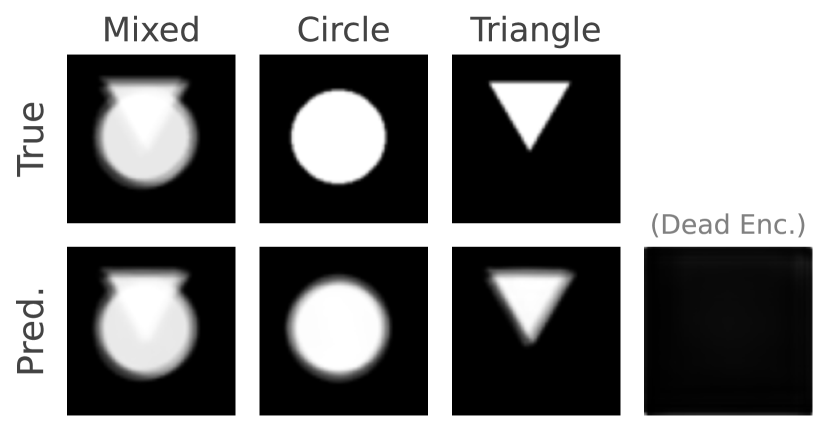
(a)

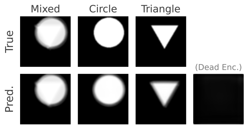
(b)

Figure 4: Sample predictions from the triangles & circles dataset experiment.

Evaluation and Analysis

Figure 4 shows two samples with the predicted reconstruction and source estimations from the trained model along with the ground truth mixture and sources (a video showing the training progression can be found in the supplementary material). Despite the non-linear mixing of sources and never having any direct or indirect supervision that uses the ground truth circle and triangle sources, the network learns to reconstruct a surprisingly accurate representation of the sources. Nevertheless, the distortion caused by the design of the mixing system is still somewhat present. Displayed along with the triangle and circle source estimations is the output that results from decoding the output of the third encoder. As expected, this third encoding pathway ultimately becomes a dead encoding space because there are only two sources that can be modeled. In terms of source reconstruction error, an average absolute validation error of $0.021$ between the true and predicted triangle sources and an average absolute validation error of $0.025$ between the true and predicted circle sources is achieved (a worst-case mean absolute error would be a value of $1.0$). For reference, the average absolute validation error of the mixed signal reconstruction is $0.006$ an order of magnitude smaller than the source reconstructions but the results are still acceptable. The final errors and the results shown in Figure 4 highlight a key limitation of the proposed method: Source estimations are in part limited by the features that the decoder can express. However, this is a common limitation of many BSS techniques as the features of the true source signals may not be knowable or fully expressed for non-linear mixtures.

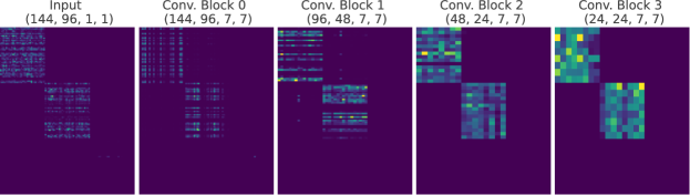
Figure 5: Visualization of weights in the decoder after training a model on the triangles & circles dataset with the proposed method.

In Figure 5, the absolute values of the weights for each layer in the decoder are summed along the spatial dimensions, and the decoder input layer is transposed. The application of the pathway separation loss is apparent, but in the second convolutional block’s weights (labeled Conv. Block 1) there are clear sparse connections shared between the encoding pathway blocks associated with the triangle and circle sources. These shared connections establish the relationship between the two source encoding spaces within the remixing or decoding process. The third encoding pathway (bottom right of each weight) is also noted to have absolute values close to zero relative to the other pathway blocks throughout the decoder indicating a dead encoding space as described in subsection 3.2.

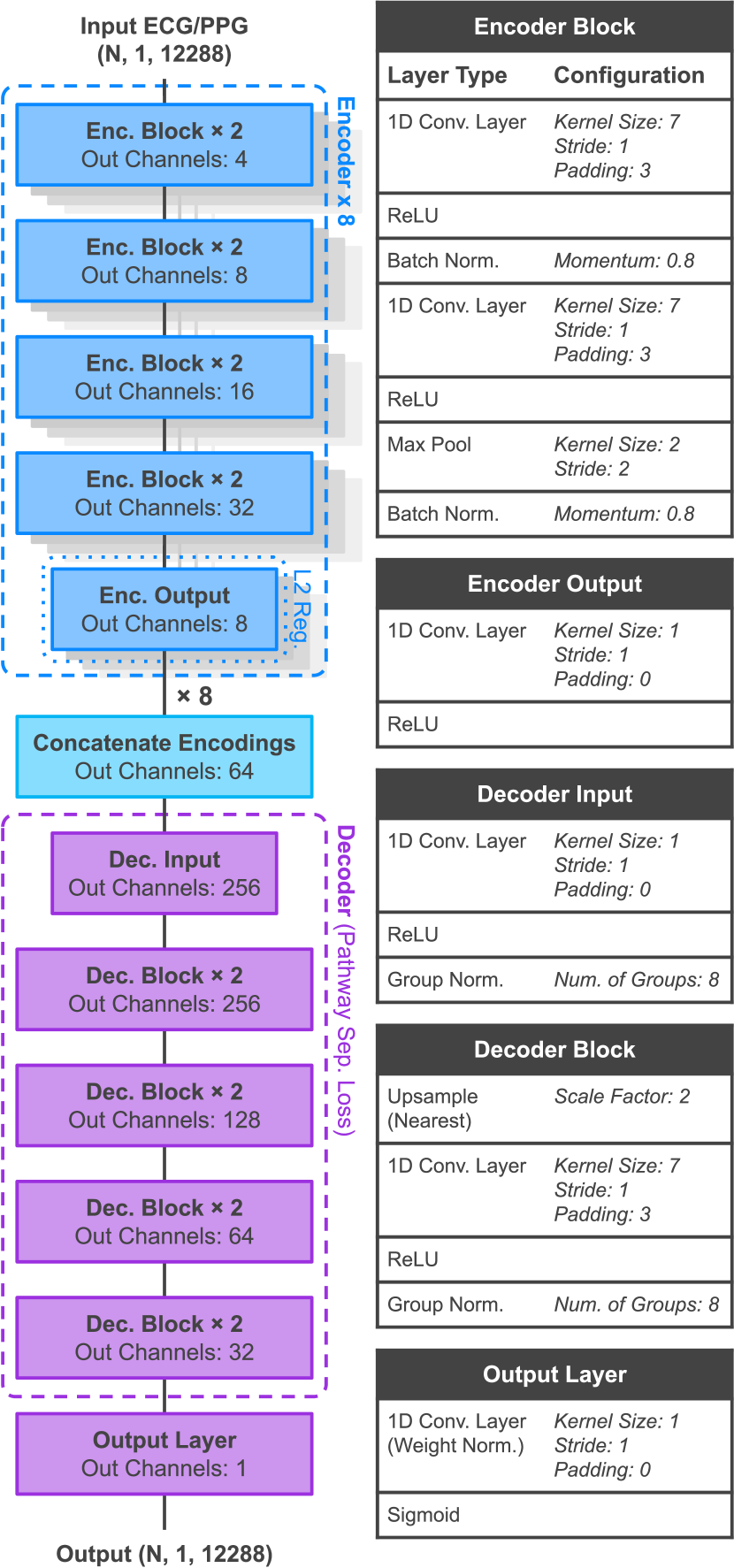
(a) ECG/PPG model experiment specifications.

(b) Triangles & circles dataset experiment model specifications.

Figure 6: Model specifications for the ECG/PPG experiments and the triangles & circles dataset experiments.

4.2 ECG and PPG Respiratory Source Extraction

Two practical experiments using real-world biosignal recordings from a polysomnography sleep study are conducted using the proposed method. Specifically, the blind source separation of respiration source signals from raw electrocardiogram (ECG) and photoplethysmography (PPG) signals, which are typically used for the analyses of cardiovascular health, are considered. There is a vast literature on extracting respiratory rate or respiration signals from ECG and PPG using various heuristic, analytical, or source separation techniques [31, 4, 49, 36, 1, 8, 34, 25, 50]. However, BSS methods applied to respiration extraction from ECG or PPG are challenging because the cardiovascular and respiratory sources may not be assumed linearly separable and may be correlated in time. ECG or PPG signals may be influenced by respiratory-induced amplitude modulation, frequency modulation, or baseline wander at different times in a signal depending on a number of physiological factors such as respiratory sinus arrhythmia [12], or the various mechanical effects of respiration on the position and orientation of the heart [45]. For these reasons, many BSS methods would fail to separate the cardiovascular and respiratory sources in a meaningful way, and thus heuristics and strong priors are often relied upon for respiration signal extraction. The proposed method has an advantage in that highly non-linear mixtures can be modeled without strong priors.

Data Specifications

The Multi-Ethnic Study of Atherosclerosis (MESA) [55, 6] is a research project funded by the NHLBI that involves six collaborative centers and investigates the factors associated with the development and progression of cardiovascular disease. The MESA Sleep study provides raw polysomnography data which includes simultaneously measured ECG, PPG, and other respiratory-related signals. Photoplethysmography (PPG) signals capture changes in blood volume and are used for measuring heart rate, oxygen saturation, and other cardiovascular parameters. Electrocardiography (ECG) signals record the heart’s electrical activity and are used to assess cardiac rhythm, detect abnormalities, and diagnose cardiac conditions. Both PPG and ECG signals play important roles in monitoring and diagnosing cardiovascular health.

From the polysomnography data, raw PPG and ECG signals are extracted for the purpose of separating a respiratory source using the proposed method which is done without the supervision of a reference respiratory source or the use of any heuristics or strong priors. Thoracic excursion recordings, which measure the expansion of the chest cavity, and nasal pressure recordings, which measure the change in airflow through the nasal passage, are extracted as reference respiratory signals for verifying the quality of the predicted respiratory source separations. For this work, $1,000$ recordings of the total $2,056$ polysomnography recordings are randomly selected from the MESA polysomnography dataset. Then, after randomly shuffling the recordings, the first $500$ recordings of this subset are used for training and the remainder are used for validation. As a first step, the PPG and ECG recordings for each polysomnography recording are resampled from the original 256hz to 200hz. Then each recording is divided into segments that are $12,288$ samples in length, or approximately $60$ seconds. As a final step, the segments are scaled using min-max scaling. No other processing or filtering is applied to the segments, however, some segments are removed if the segment appears to have physiologically impossible characteristics i.e. the extracted heart rate is too high or too low. For evaluation of the extracted respiratory sources, the NeuroKit2 open source library [30] is used to process the respiratory signals and then extract the respiratory rate. For inference, the two ends of the source estimations are clipped as the edges tend to produce noise that is much higher in amplitude than source signal representations found towards the center.

Model Specifications

For both the ECG and PPG experiments, the same fully convolutional multi-encoder autoencoder, detailed in 6(a), is trained using the proposed method. The Adam optimizer with a learning rate of $1\times 10^{-3}$ is used for optimizing the model weights. Additionally, a weight decay of $1\times 10^{-6}$ is applied over all parameters. The scalars for the additional regularization terms, $\lambda_{\text{pathway}}$, $\lambda_{\text{zero recon.}}$, and $\lambda_{\text{z}}$, are set to $1\times 10^{-3}$, $1\times 10^{-2}$, and $1\times 10^{-2}$, respectively. The batch size is set to $256$ segments. The models for both PPG and ECG are trained for $50$ epochs, and then the best-performing model from these runs is chosen for the final evaluation on the test set.

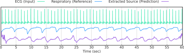
(a) ECG respiration extraction via proposed BSS method.

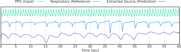
(b) PPG respiration extraction via proposed BSS method.

Figure 7: Sample graphs showing our extracted respiration sources from PPG and ECG along with a simultaneously measured reference respiratory signal.

Evaluation and Analysis

In Figure 7, a simultaneously measured reference respiration signal, and the extracted respiration source signal using our method are visualized for both ECG and PPG experiments (more samples are in the supplementary material). In 7(a) the reference respiration signal shown is thoracic excursion, and for 7(b) the reference respiratory signal is nasal pressure. While the predicted respiratory source and the thoracic excursion signal are often well correlated, they represent slightly different physiological processes. The predicted source is an estimated representation of the respiratory-related movement feature subspace within the mixed input signals, ECG or PPG. Thus the predicted respiratory source and a reference respiration signal may have subtle or obvious differences in feature expression. For example, the predicted respiration source may have unique amplitude modulation patterns or appear flipped relative to the respiration reference as seen in 7(a). For these reasons, the proposed method is evaluated by extracting respiratory rate from the predicted source signals and for two reference respiratory signals, nasal flow and thoracic excursion, which is achieved by measuring the periods between inhalation onsets or troughs for one-minute segments. Then the mean absolute error (MAE) between the respiratory rates of each of the source estimations and each of the reference signals is calculated to determine the degree to which the predicted respiration sources preserve respiratory information.

Table 1: The test mean absolute error (MAE) in breaths per minute between each method of respiratory signal extraction (our method, the competing heuristic approaches, and two additional baselines), and the two reference respiratory signals.

Method (Type)	Breaths/Min. MAE $\downarrow$		Method (Type)	Breaths/Min. MAE $\downarrow$
BSS	Nasal Press.	Thor.	Heuristic	Nasal Press.	Thor.
Ours (PPG)	1.51	1.50	[31] (ECG)	2.38	2.04
Ours (ECG)	1.73	1.59	[4] (ECG)	2.38	2.05
			[49] (ECG)	2.27	1.95
			[36] (ECG)	2.26	1.94
Supervised			Direct Comparison
AE (PPG)	0.46 (0.87)	2.07 (1.71)	Thor.	1.33	–
AE (ECG)	0.48 (1.03)	2.16 (1.69)

The experimental results in Table 1 show the test mean absolute error (MAE) in breaths per minute between each method of respiratory signal extraction and the two reference respiratory signals, nasal pressure and thoracic excursion (abbreviated as nasal press. and thor.) where type refers to the input signal that the method extracts the respiratory signal from, either ECG or PPG. The primary result shows that the proposed method for BSS performs better than the competing heuristic approaches designed specifically for the task of respiratory signal extraction. Two additional baselines are included as a point of reference: the results of a supervised model trained to predict the nasal pressure signal from the two types of input signals (similar to other works [1, 8, 34]) and a direct comparison between the thoracic excursion signal and nasal flow signal. The supervised approach, employing a standard autoencoder (AE) architecture, generally performs well at predicting the reference respiratory signal it is trained to reconstruct, nasal pressure, but generalizes poorly to the other reference respiratory signal, thoracic excursion. Early-stopping does result in better generalization (shown in parenthesis next to the primary result). However, for many tasks where BSS is applied, a supervised approach is usually not viable because reference signals for sources may not be available, though having reference signals was essential for the evaluation of our method in this paper.

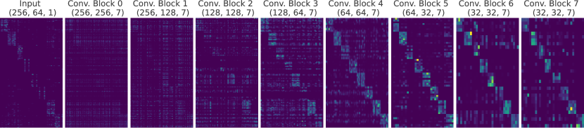
(a) Absolute values of ECG model decoder weights.

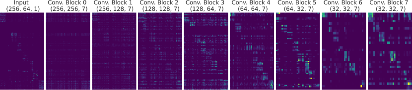
(b) Absolute values of PPG model decoder weights.

Figure 8: The absolute values of the decoder weights summed along the spatial dimension for the PPG and ECG models showing the application of the pathway separation loss.

The absolute values of the decoder weights summed along the spatial dimension for the PPG and ECG models are shown in Figure 8. Due to the complex non-linear relationships that occur between sources in a PPG or ECG signal, a lower penalty is applied to the pathway separation loss, and the alternative $\alpha$ scalar (13) is applied. Thus, the weights within the off-diagonal pathway blocks have generally higher values in comparison to the model trained for the triangles & circles dataset experiment.

4.3 Code Availability

Our implementation of the experiments described in this paper is available on GitHub at the following link: github.com/webstah/self-supervised-bss-via-multi-encoder-ae.

5 Conclusion

The method for BSS using multi-encoder autoencoders introduced in this paper presents a novel data-driven solution to BSS without strong application-specific priors or the assumption that sources are linearly separable from the given mixture. The ability of the separate encoders to discover the feature subspaces of sources and of the decoder to reconstruct those sources was demonstrated. In addition, this work demonstrates that the proposed method does not have a limitation in the number of sources that can be separated. Overestimating the number of sources with more encoders than is truly necessary simply leads to dead encoders, however, there are some key limitations. Due to the nature of the BSS task, it is not possible to know if the extracted sources are true representations of the sources. As seen in the triangles & circles dataset experiment, the distortion applied by the mixing system is not fully removed from the reconstructed sources. Future works exploring these issues can lead to improved results as well as enhance the understanding of the proposed method in relation to the BSS task.

5.1 Broader Impact Statement

While this work shows that meaningful source separation occurs with the ECG and PPG experiments, the ability of the proposed method, or any BSS approach, to reconstruct exact sources should not be overstated and this fact must be taken into consideration before applying the proposed method in any real-world context especially those involving medical diagnosis or decisions that may negatively impact any individuals, demographics, or society as a whole. Further investigation is necessary to understand the shortcomings of the proposed method despite the positive results presented in this paper.

5.2 Acknowledgements

We want to express our sincere thanks to Dr. Masoud R. Hamedani and Dr. M. Dujon Johnson for their help in editing and providing valuable suggestions to enhance the clarity and flow of this paper. Additionally, we thank Dr. Jeremy Wurbs for their engaging discussions that helped kick-start our research journey.

This work was supported by the Technology Development Program (S3201499) funded by the Ministry of SMEs and Startups (MSS, Korea).

The Multi-Ethnic Study of Atherosclerosis (MESA) Sleep Ancillary study was funded by NIH-NHLBI Association of Sleep Disorders with Cardiovascular Health Across Ethnic Groups (RO1 HL098433). MESA is supported by NHLBI funded contracts HHSN268201500003I, N01-HC-95159, N01-HC-95160, N01-HC-95161, N01-HC-95162, N01-HC-95163, N01-HC-95164, N01-HC-95165, N01-HC-95166, N01-HC-95167, N01-HC-95168 and N01-HC-95169 from the National Heart, Lung, and Blood Institute, and by cooperative agreements UL1-TR-000040, UL1-TR-001079, and UL1-TR-001420 funded by NCATS. The National Sleep Research Resource was supported by the National Heart, Lung, and Blood Institute (R24 HL114473, 75N92019R002).

References

- [1] Aqajari, S. A. H., Cao, R., Zargari, A. H. A., and Rahmani, A. M. An end-to-end and accurate ppg-based respiratory rate estimation approach using cycle generative adversarial networks. In 2021 43rd Annual International Conference of the IEEE Engineering in Medicine & Biology Society (EMBC) (2021), pp. 744–747.
- [2] Barros, A. K., Mansour, A., and Ohnishi, N. Removing artifacts from electrocardiographic signals using independent components analysis. Neurocomputing 22, 1 (1998), 173–186.
- [3] Bell, A., and Sejnowski, T. An information-maximization approach to blind separation and blind deconvolution. Neural computation 7 (12 1995), 1129–59.
- [4] Charlton, P. H., Bonnici, T., Tarassenko, L., Clifton, D. A., Beale, R., and Watkinson, P. J. An assessment of algorithms to estimate respiratory rate from the electrocardiogram and photoplethysmogram. Physiological Measurement 37, 4 (mar 2016), 610.
- [5] Chen, J., Mao, Q., and Liu, D. Dual-Path Transformer Network: Direct Context-Aware Modeling for End-to-End Monaural Speech Separation. In Proc. Interspeech 2020 (2020), pp. 2642–2646.
- [6] Chen, X., Wang, R., Zee, P., Lutsey, P. L., Javaheri, S., Alcántara, C., Jackson, C. L., Williams, M. A., and Redline, S. Racial/ethnic differences in sleep disturbances: The multi-ethnic study of atherosclerosis (mesa). Sleep 38, 6 (06 2015), 877–888.
- [7] Chen, Z., Luo, Y., and Mesgarani, N. Deep attractor network for single-microphone speaker separation. 2017 IEEE International Conference on Acoustics, Speech and Signal Processing (ICASSP) (2016), 246–250.
- [8] Davies, H. J., and Mandic, D. P. Rapid extraction of respiratory waveforms from photoplethysmography: A deep corr-encoder approach. Biomedical Signal Processing and Control 85 (2023), 104992.
- [9] Gandelsman, Y., Shocher, A., and Irani, M. "double-dip": Unsupervised image decomposition via coupled deep-image-priors. In Proceedings of the IEEE/CVF Conference on Computer Vision and Pattern Recognition (CVPR) (June 2019).
- [10] Hershey, J. R., Chen, Z., Le Roux, J., and Watanabe, S. Deep clustering: Discriminative embeddings for segmentation and separation. In 2016 IEEE International Conference on Acoustics, Speech and Signal Processing (ICASSP) (2016), pp. 31–35.
- [11] Hinton, G. E., and Salakhutdinov, R. R. Reducing the dimensionality of data with neural networks. Science 313, 5786 (2006), 504–507.
- [12] Hirsch, J. A., and Bishop, B. P. Respiratory sinus arrhythmia in humans: how breathing pattern modulates heart rate. The American journal of physiology 241 4 (1981), H620–9.
- [13] Hoshen, Y. Towards unsupervised single-channel blind source separation using adversarial pair unmix-and-remix. In ICASSP 2019 - 2019 IEEE International Conference on Acoustics, Speech and Signal Processing (ICASSP) (2019), pp. 3272–3276.
- [14] Hyvarinen, A. Fast and robust fixed-point algorithms for independent component analysis. IEEE Transactions on Neural Networks 10, 3 (1999), 626–634.
- [15] Hyvärinen, A. Independent component analysis: recent advances. Philosophical Transactions of the Royal Society A: Mathematical, Physical and Engineering Sciences 371, 1984 (2013), 20110534.
- [16] Hyvärinen, A., and Oja, E. Independent component analysis: algorithms and applications. Neural Networks 13, 4 (2000), 411–430.
- [17] Ioffe, S., and Szegedy, C. Batch normalization: Accelerating deep network training by reducing internal covariate shift. In Proceedings of the 32nd International Conference on Machine Learning (Lille, France, 07–09 Jul 2015), F. Bach and D. Blei, Eds., vol. 37 of Proceedings of Machine Learning Research, PMLR, pp. 448–456.
- [18] Jayaram, V., and Thickstun, J. Source separation with deep generative priors. In Proceedings of the 37th International Conference on Machine Learning (13–18 Jul 2020), H. D. III and A. Singh, Eds., vol. 119 of Proceedings of Machine Learning Research, PMLR, pp. 4724–4735.
- [19] Kameoka, H., Li, L., Inoue, S., and Makino, S. Supervised determined source separation with multichannel variational autoencoder. Neural Computation 31, 9 (09 2019), 1891–1914.
- [20] Karhunen, J., Pajunen, P., and Oja, E. The nonlinear pca criterion in blind source separation: Relations with other approaches. Neurocomputing 22, 1 (1998), 5–20.
- [21] Kofidis, E. Blind source separation: Fundamentals and recent advances (a tutorial overview presented at sbrt-2001), 2016.
- [22] Krizhevsky, A., Sutskever, I., and Hinton, G. E. Imagenet classification with deep convolutional neural networks. Communications of the ACM 60, 6 (2012), 84–90.
- [23] Lee, D. D., and Seung, H. S. Learning the parts of objects by non-negative matrix factorization. Nature 401, 6755 (1999), 788–791.
- [24] Lee, K. J., and Lee, B. End-to-end deep learning architecture for separating maternal and fetal ecgs using w-net. IEEE Access 10 (2022), 39782–39788.
- [25] Lipsitz, L. A., Hashimoto, F., Lubowsky, L. P., Mietus, J. E., Moody, G. B., Appenzeller, O., and Goldberger, A. L. Heart rate and respiratory rhythm dynamics on ascent to high altitude. British Heart Journal 74 (1995), 390 – 396.
- [26] Liu, Y., and Lu, F. Separate in latent space: Unsupervised single image layer separation. In Proceedings of the AAAI Conference on Artificial Intelligence (2020), vol. 34, pp. 11661–11668.
- [27] Luo, Y., Chen, Z., and Yoshioka, T. Dual-path rnn: Efficient long sequence modeling for time-domain single-channel speech separation. In ICASSP 2020 - 2020 IEEE International Conference on Acoustics, Speech and Signal Processing (ICASSP) (2020), pp. 46–50.
- [28] Luo, Y., and Mesgarani, N. Tasnet: Time-domain audio separation network for real-time, single-channel speech separation. 2018 IEEE International Conference on Acoustics, Speech and Signal Processing (ICASSP) (2017), 696–700.
- [29] Luo, Y., and Mesgarani, N. Conv-tasnet: Surpassing ideal time-frequency magnitude masking for speech separation. IEEE/ACM Transactions on Audio, Speech, and Language Processing PP (05 2019), 1–1.
- [30] Makowski, D., Pham, T., Lau, Z. J., Brammer, J. C., Lespinasse, F., Pham, H., Schölzel, C., and Chen, S. H. A. NeuroKit2: A python toolbox for neurophysiological signal processing. Behavior Research Methods 53, 4 (feb 2021), 1689–1696.
- [31] Muniyandi, M., and Soni, R. Breath rate variability (brv) - a novel measure to study the meditation effects. International Journal of Yoga Accepted (01 2017).
- [32] Neri, J., Badeau, R., and Depalle, P. Unsupervised blind source separation with variational auto-encoders. In 2021 29th European Signal Processing Conference (EUSIPCO) (2021), pp. 311–315.
- [33] Ong, Y. Z., Chui, C. K., and Yang, H. Cass: Cross adversarial source separation via autoencoder. ArXiv abs/1905.09877 (2019).
- [34] Ravichandran, V., Murugesan, B., Balakarthikeyan, V., Ram, K., Preejith, S., Joseph, J., and Sivaprakasam, M. Respnet: A deep learning model for extraction of respiration from photoplethysmogram. In 2019 41st Annual International Conference of the IEEE Engineering in Medicine and Biology Society (EMBC) (2019), pp. 5556–5559.
- [35] Rouard, S., Massa, F., and Défossez, A. Hybrid transformers for music source separation, 2022.
- [36] S. Sarkar, S. Bhattacherjee, S. P. Extraction of respiration signal from ecg for respiratory rate estimation. IET Conference Proceedings (January 2015), 58 (5 .)–58 (5 .)(1).
- [37] Salimans, T., and Kingma, D. P. Weight normalization: A simple reparameterization to accelerate training of deep neural networks, 2016.
- [38] Samuel, D., Ganeshan, A., and Naradowsky, J. Meta-learning extractors for music source separation. ICASSP 2020 - 2020 IEEE International Conference on Acoustics, Speech and Signal Processing (ICASSP) (2020), 816–820.
- [39] Shokouhmand, A., and Tavassolian, N. Fetal electrocardiogram extraction using dual-path source separation of single-channel non-invasive abdominal recordings. IEEE Transactions on Biomedical Engineering 70, 1 (2023), 283–295.
- [40] Singh, A., and Ogunfunmi, T. An overview of variational autoencoders for source separation, finance, and bio-signal applications. Entropy 24, 1 (2022).
- [41] Stadlthanner, K., Theis, F. J., Lang, E. W., Tomé, A. M., Puntonet, C. G., Vilda, P. G., Langmann, T., and Schmitz, G. Sparse nonnegative matrix factorization applied to microarray data sets. In Independent Component Analysis and Blind Signal Separation (Berlin, Heidelberg, 2006), J. Rosca, D. Erdogmus, J. C. Príncipe, and S. Haykin, Eds., Springer Berlin Heidelberg, pp. 254–261.
- [42] Stoller, D., Ewert, S., and Dixon, S. Adversarial semi-supervised audio source separation applied to singing voice extraction. In 2018 IEEE International Conference on Acoustics, Speech and Signal Processing (ICASSP) (2018), IEEE, pp. 2391–2395.
- [43] Stoller, D., Ewert, S., and Dixon, S. Wave-u-net: A multi-scale neural network for end-to-end audio source separation. In Proceedings of the 19th International Society for Music Information Retrieval Conference, ISMIR 2018, Paris, France, September 23-27, 2018 (2018), E. Gómez, X. Hu, E. Humphrey, and E. Benetos, Eds., pp. 334–340.
- [44] Subakan, C., Ravanelli, M., Cornell, S., Bronzi, M., and Zhong, J. Attention is all you need in speech separation. In ICASSP 2021 - 2021 IEEE International Conference on Acoustics, Speech and Signal Processing (ICASSP) (2021), pp. 21–25.
- [45] Surawicz, B., and Knilans, T. Chou’s electrocardiography in clinical practice: adult and pediatric. Elsevier Health Sciences, 2008.
- [46] Tang, G., Müller, M., Rios, A., and Sennrich, R. Why self-attention? a targeted evaluation of neural machine translation architectures. In Proceedings of the 2018 Conference on Empirical Methods in Natural Language Processing (Brussels, Belgium, Oct.-Nov. 2018), Association for Computational Linguistics, pp. 4263–4272.
- [47] Ternes, L., Dane, M., Gross, S., and et al. A multi-encoder variational autoencoder controls multiple transformational features in single-cell image analysis. Commun Biol 5 (2022), 255.
- [48] Umesh, P. Image processing in python. CSI Communications 23 (2012).
- [49] van Gent, P., Farah, H., van Nes, N., and van Arem, B. Heartpy: A novel heart rate algorithm for the analysis of noisy signals. Transportation Research Part F: Traffic Psychology and Behaviour 66 (2019), 368–378.
- [50] Varon, C., Morales, J., Lazaro, J., Orini, M., Deviaene, M., Kontaxis, S., Testelmans, D., Buyse, B., Borzée, P., Sörnmo, L., Laguna, P., Gil, E., and Bailón, R. A comparative study of ecg-derived respiration in ambulatory monitoring using the single-lead ecg. Scientific Reports 10 (03 2020), 5704.
- [51] Vaswani, A., Shazeer, N., Parmar, N., Uszkoreit, J., Jones, L., Gomez, A. N., Kaiser, Ł., and Polosukhin, I. Attention is all you need. In Proceedings of the 31st International Conference on Neural Information Processing Systems (2017), pp. 6000–6010.
- [52] Voita, E., Serdyukov, P., Sennrich, R., and Titov, I. Context-aware neural machine translation learns anaphora resolution. In Proceedings of the 56th Annual Meeting of the Association for Computational Linguistics (Volume 1: Long Papers) (Melbourne, Australia, July 2018), Association for Computational Linguistics, pp. 1264–1274.
- [53] Voita, E., Talbot, D., Moiseev, F., Sennrich, R., and Titov, I. Analyzing multi-head self-attention: Specialized heads do the heavy lifting, the rest can be pruned. In Proceedings of the 57th Annual Meeting of the Association for Computational Linguistics (Florence, Italy, jul 2019), Association for Computational Linguistics, pp. 5797–5808.
- [54] Wu, Y., and He, K. Group normalization. In Proceedings of the European Conference on Computer Vision (ECCV) (September 2018).
- [55] Zhang, G.-Q., Cui, L., Mueller, R., Tao, S., Kim, M., Rueschman, M., Mariani, S., Mobley, D., and Redline, S. The national sleep research resource: Towards a sleep data commons. Journal of the American Medical Informatics Association 25, 10 (10 2018), 1351–1358.
- [56] Zhao, M., Yao, X., Wang, J., Yan, Y., Gao, X., and Fan, Y. Single-channel blind source separation of spatial aliasing signal based on stacked-lstm. Sensors 21, 14 (2021).
- [57] Zhao, S., and Ma, B. Mossformer: Pushing the performance limit of monaural speech separation using gated single-head transformer with convolution-augmented joint self-attentions. CoRR abs/2302.11824 (2023).
- [58] Zou, Z., Lei, S., Shi, T., Shi, Z., and Ye, J. Deep adversarial decomposition: A unified framework for separating superimposed images. In Proceedings of the IEEE/CVF Conference on Computer Vision and Pattern Recognition (CVPR) (June 2020).