Masked Transformer for Electrocardiogram Classification

Abstract

Electrocardiogram (ECG) is one of the most important diagnostic tools in clinical applications. With the advent of advanced algorithms, various deep learning models have been adopted for ECG tasks. However, the potential of Transformers for ECG data is not yet realized, despite their widespread success in computer vision and natural language processing. In this work, we present a useful masked Transformer method for ECG classification referred to as MTECG, which expands the application of masked autoencoders to ECG time series. We construct a dataset comprising 220,251 ECG recordings with a broad range of diagnoses annoated by medical experts to explore the properties of MTECG. Under the proposed training strategies, a lightweight model with 5.7M parameters performs stably well on a broad range of masking ratios (5%-75%). The ablation studies highlight the importance of fluctuated reconstruction targets, training schedule length, layer-wise LR decay and DropPath rate. The experiments on both private and public ECG datasets demonstrate that MTECG-T significantly outperforms the recent state-of-the-art algorithms in ECG classification.

Keywords: Electrocardiogram, Transformer, Masked autoencoders, Classification

1 Introduction

The electrocardiogram (ECG) is one of the most commonly used non-invasive tools in clinical applications, recording the cardiac electrical activity and providing valuable diagnostic clues for systemic conditions (Siontis et al., 2021). With the algorithmic advances in computer vision (CV) several years ago, convolutional neural networks (CNN) have been adapted to solve various ECG classification tasks, such as detecting arrhythmia (Hannun et al., 2019; Ribeiro et al., 2020; Hughes et al., 2021), left ventricular systolic dysfunction (Attia et al., 2019, 2022; Yao et al., 2021) and hypertrophic cardiomyopathy (Ko et al., 2020).

The field of CV has been transformed recently by the excellent performance of Transformer models (Vaswani et al., 2017; Dosovitskiy et al., 2020). However, the progress of Transformer methods for ECG tasks lags behind those in CV. CNN remain the most common architecture for ECG data analysis (Siontis et al., 2021; Somani et al., 2021). A natural question is that can Transformer also be leveraged for ECG tasks. We attempt to answer the question in this paper.

One challenge is to adapt Transformers to effectively model ECG data. Commonly used ECG data are time-series signals with a unique temporal and spatial structure. For example, the standard 10 seconds 12-lead ECG signals with 500Hz sampling rate have 5000 time points. These signals typically consist of several beats with multiple waves, such as the P wave, QRS complex, T wave, and sometimes U wave (Sharma and Sunkaria, 2021). Directly modeling each time step individually in Transformer might ruin the structural information and lead to heavy computation. One possible solution is to split the signal into a sequence of non-overlapping segments (Li et al., 2021). The structural information could be preserved in the segments and the sequence length could be remarkably reduced. Treating these segments as tokens or image patches, we can easily utilize the design of Vision Transformer (ViT, Dosovitskiy et al., 2020).

Another challenge is the lack of available labeled datasets. It is known that the successful training of Transformers requires a large-scale dataset with labeled data, e.g., ImageNet-21k (Deng et al., 2009), due to the lack of inductive bias (Dosovitskiy et al., 2020). However, creating labeled ECG datasets at scale is challenging since accurate annotation requires medical experts and considerable time. Although recent advancements have introduced larger ECG datasets like PTB-XL (Wagner et al., 2020) and Chapman-Shaoxing (Zheng et al., 2020b), they still contain only a few tens of thousands of data points, making the Transformer model prone to overfitting (Li et al., 2021). To address this limitation, we build a comprehensive dataset comprising 220,251 ECG recordings with a broad range of ECG diagnoses annotated by medical experts.

Although the constructed dataset is much larger than publicly available ECG datasets, our experiments show that naively training Transformers yields unsatisfactory results. We still encoder overfitting, even for a lightweight Transformer with 5.7M parameters. This problem might caused by the information redundancy (Wei et al., 2019), which typically exists in ECG time series. For example, each time point can be inferred from neighboring points, and some heartbeat cycles could be inferred from neighboring heartbeat cycles. For natural image, the information redundancy has been effectively addressed by masked modeling methods (He et al., 2022; Xie et al., 2022), a popular class of self-supervised learning method.

Inspired by their success, we propose a masked Transformer method for ECG classification, referred as MTECG. We split the ECG signal into a sequence of non-overlapping segments and adopt learnable positional embeddings to preserve the sequential order information and distinguish the segments. The masked pre-training on the unlabeled ECG data is used to reduce information redundancy. To encourage the encoder learning useful wave shape features, we adopt a lightweight decoder and a fluctuated reconstruction target in the pre-training stage. To further reduce overfitting, we explore the regularization strategies such as layer-wise LR decay (Bao et al., 2021; Clark et al., 2020) and DropPath (Huang et al., 2016) rate in the fine-tuning stage. Noting that the model capacity matters to the generalization ability and the clinical application, we also conduct experiments on the encoder of different sizes to explore an appropriate setting.

The main contributions of this work are summarized as follows.

1. Novel Application: We propose MTECG, a useful masked Transformer method for ECG time series, as the extension of MAE originally proposed for the natural image analysis (He et al., 2022). The derived lightweight models stemming from the vanilla ViT demonstrate the ability to classify a wide range of ECG diagnoses effectively, while remaining convenient for deployment in the clinical environment.

2. New Dataset: We build a comprehensive ECG dataset to evaluate the deep learning algorithms. The dataset consists of 220,251 recordings with 28 common ECG diagnoses annotated by medical experts and significantly surpasses the sample size of publicly available ECG datasets.

3. Strong Pre-training and Fine-tuning Recipe: We conduct comprehensive experiments to explore the training strategies on the proposed ECG dataset. The key components contributing to the proposed method are presented, including the masking ratio, training schedule length, fluctuated reconstruction target, layer-wise LR decay and DropPath rate.

4. Excellent Performance: We compare the proposed method with three recent state-of-the-art algorithms on a wide variety of tasks in both private and public ECG datasets. The experiments demonstrate that the proposed algorithm outperforms others significantly.

The rest of this article is organized as follows. Section 2 briefly outlines the related works. Section 3 introduces the proposed method. The experiment setting, the properties and the practical performance of the proposed method can be founded in Section 4. We provide the additional discussion in Section 5. The conclusion of this work is summarized in Section 6.

2 Related work

2.1 ECG classification

ECG classification is one of the most important ECG data analysis tasks (Pyakillya et al., 2017; Somani et al., 2021; Siontis et al., 2021). Traditionally, the classification for ECG signals is mainly based on expert features and conventional machine learning methods (Hong et al., 2020). However, the algorithm performance is limited by data quality and expert knowledge (Hong et al., 2020), precluding the usage in clinical applications (Ribeiro et al., 2020). To overcome these limitations, numerous works have adapted end-to-end deep learning approaches to ECG tasks (Hannun et al., 2019). In comparison to the traditional methods, the deep learning approach can automatically learn useful features from raw ECG signals and achieve better performance in many classification tasks (Strodthoff et al., 2023).

2.2 Transformer

Transformer is an attention-based architecture which rapidly becomes the dominant choice in natural language processing (NLP) since it was proposed (Vaswani et al., 2017; Devlin et al., 2019; Radford et al., 2018). Due to the excellent performance, the filed of CV has also been transformed recently by Transformer (Han et al., 2022; Khan et al., 2022). Compared to CNN, Transformer can better utilize the global structure of the data and share shape recognition properties of the human visual system (Naseer et al., 2021). However, CNN still remains the most common architecture for ECG data analysis (Somani et al., 2021). Although some works have made attempts on Transformer-based models, such as BaT (Li et al., 2021) and MaeFE (Zhang et al., 2022), the comprehensive evaluation remains lacking and the potential is still not fully realized. We will compare the performance of the proposed method with BaT and MaeFE.

2.3 Self-supervised learning

Self-supervised learning is a popular method to utilize the unlabeled data and enhance the algorithm performance (Liu et al., 2021). Contrastive and generative learning are two main self-supervised learning approaches (Krishnan et al., 2022), and various contrastive learning methods have been proposed for ECG data analysis (Chen et al., 2021; Kiyasseh et al., 2021; Oh et al., 2022; Mehari and Strodthoff, 2022). This type of methods aim at modeling the sample similarity and dissimilarity through a contrastive estimation objective (Gutmann and Hyvärinen, 2010; Liu et al., 2021) and the performance heavily relies on the data augmentation strategy (He et al., 2022; Wang et al., 2023b). Generative learning, such as GPT (Radford et al., 2018), BERT(Devlin et al., 2019), BEiT (Bao et al., 2021) and MAE (He et al., 2022), is another main self-supervised learning method. Although it gains steadily increasing attention in NLP and CV, the number of works for ECG tasks is limited. A recent work has made attempts on masked modeling for ECG data and proposed MaeFE (Zhang et al., 2022).

3 Methodology

Our approach expands image MAE (He et al., 2022) to ECG time series and follows the pretrain-and-finetune paradigm. The framework consists of 5 major components, i.e., segment operation, mask operation, encoder, decoder, and reconstruction target. As shown in Figure 1, the pre-training stage involves all components. As for fine-tuning, the decoder, reconstruction target and mask operation will be discarded. In the subsequent subsections, we detail each component and the training strategy.

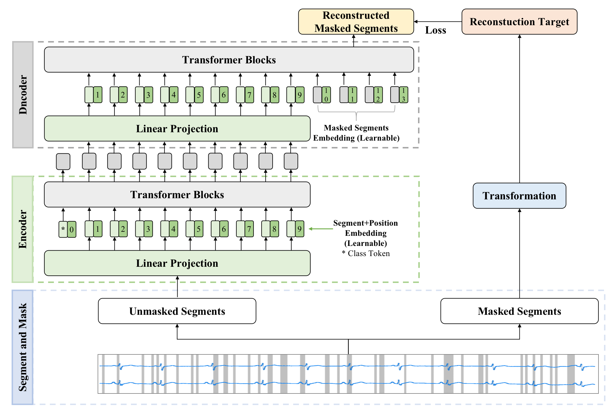
Figure 1: An example of the masked pre-training method. The original ECG signals are split to non-overlapping segments and a subset of these segments is masked out. The unmasked segments were used to reconstruct the fluctuated transformation of the masked segments through Transformer blocks. The lead and sequence information of the ECG signals are preserved by learnable positional embeddings. The masked segments are represented by learnable embeddings in the reconstruction task.

3.1 Segment operation

For simplicity, this paper focuses on fixed-length ECG data. This type of ECG signal can be denoted as $\bm{X}^{\sharp}=(X_{k,q}^{\sharp})\in\mathbb{R}^{K\times Q}$, where $K$ is the number of leads and $Q$ is the length of ECG. In many applications, $Q$ is much larger than $K$. For example, in the case of standard 12-lead ECGs, with a duration of 10 seconds and a sampling frequency of 500 Hz, we have $Q=5000$ and $K=12$. When dealing with ECG signals of this length, directly modeling each time step individually using a Transformer would lead to heavy computation due to the quadratic cost of the self-attention operation. Moreover, ECG signals comprise multiple beats, each of which typically consists of various components such as the P wave, QRS complex, T wave, and U wave. If we were to model the signals at the individual time point level, we might ignore the wave shape information.

Alternatively, we split the ECG signal $\bm{X}^{\sharp}$ into a sequence of non-overlapping segments $\mathcal{S}=\{\bm{X}_{1},\ldots,\bm{X}_{T}\}$, where $T$ is the sequence length. The structural information of waves could be preserved in the segments and the sequence length could be remarkably reduced. Each segment $\bm{X}_{t}=(X_{k,q}^{t})\in\mathbb{R}^{K\times(Q/T)}$ represents a subset of the original signal, where $\bm{X}_{t}=(X_{k,q}^{t})\in\mathbb{R}^{K\times(Q/T)}$ and $X_{k,q}^{t}=X_{k,\{(t-1)*Q/T+q\}}^{\sharp}$ for $t=1,\ldots,T$, $k=1,\ldots,K,q=1,\ldots,Q/T$. These ECG segments can be regarded as image patches in computer vision, or tokens (words) in natural language processing. Similar to image MAE (He et al., 2022), we utilize a linear projection to resize the vectorization of the ECG segments. However, unlike their work, we incorporate learnable positional embeddings to preserve the sequential order information and distinguish the segments, as shown in (1) and (2).

3.2 Mask operation

As mentioned in Section 1, we employ a masked pre-training method to address information redundancy and overfitting. Specifically, we employ a uniform random sampling technique to select segments from $\mathcal{S}$ without replacement, while the remaining segments are masked. For notational simplicity, we denote the unmasked segments as

$$\mathcal{S}_{unmask}=\{\bm{X}_{i_{1}},\ldots,\bm{X}_{i_{S}}\},$$

and the masked segments as

$$\mathcal{S}_{mask}=\{\bm{X}_{j_{1}},\ldots,\bm{X}_{j_{S^{\prime}}}\},$$

Here, $i_{s}$ and $j_{s^{\prime}}$ are chosen from the set $\{1,\ldots,T\}$, with $s=1,\ldots,S$ and $s^{\prime}=1,\ldots,S^{\prime}$. The segments in $\mathcal{S}_{unmask}$ are sent to the encoder, while those in $\mathcal{S}_{mask}$ will be transformed into the reconstruction targets. Although the case $T=S+S^{\prime}$ is the main focus of this paper, the entire framework is also applicable to the case where $T<S+S^{\prime}$.

3.3 Encoder

In our settings, we can easily utilize the design of ViT (Dosovitskiy et al., 2020). We use a stack of standard Transformers (Vaswani et al., 2017; Dosovitskiy et al., 2020) as the encoder. For the natural image, MAE (He et al., 2022) incorporates vanilla positional embeddings (the sine-cosine version) to extract location information. However, previous studies demonstrate that this vanilla positional approach might be unable to fully exploit the important features of times series data (Wen et al., 2022). Therefore, we utilize learnable positional embeddings to effectively model the lead and sequence information in the ECG time series.

We briefly introduce the encoder below. Denote the layer normalization (Ba et al., 2016), the multi-headed self-attention and multi-linear perception blocks used in ViT (Dosovitskiy et al., 2020) as $LN(\cdot)$ , $MSA(\cdot)$ and $MLP(\cdot)$, respectively. We use $\bm{x}_{i_{s}}^{\intercal}\in\mathbb{R}^{KQ/T}$ to denote the vectorization of $\bm{X}_{i_{s}}$ for $s=1,\ldots,S$. Suppose $D$ is the latent vector size. Let the linear projection matrix $\bm{E}\in\mathbb{R}^{(KQ/T)\times D}$, the auxiliary token $\bm{x}_{class}^{\intercal}\in\mathbb{R}^{D}$ , and the positional embedding $\bm{e}_{pos}=(\bm{e}_{0},\bm{e}_{1},\cdots,\bm{e}_{T})^{\intercal}\in\mathbb{R}^{D(T+1)}$ be learnable. Here $\bm{e}_{t}^{\intercal}\in\mathbb{R}^{D},t=0,1,\ldots,T$ are used to preserve the sequential order information and distinguish the segments. During pre-training, only the unmasked segments are fed to the encoder, which can be written as

$$\bm{z}_{0} =[\bm{x}_{class};\bm{x}_{i_{1}}\bm{E},\cdots,\bm{x}_{i_{S}}\bm{E}]+[\bm{e}_{0};\bm{e}_{i_{1}};\ldots;\bm{e}_{i_{S}}],$$ (1)

$$\bm{z}_{l}^{\prime} =MSA(LN(\bm{z}_{l-1}))+\bm{z}_{l-1},l=1,\ldots,L,$$

$$\bm{z}_{l} =MSA(LN(\bm{z}_{l}^{\prime}))+\bm{z}_{l}^{\prime},l=1,\ldots,L,$$

where $L$ is the number of blocks. For simplicity, we denote the output $\bm{z}_{L}$ as

$$\bm{z}_{L}=[\bm{z}_{L}^{0};\bm{z}^{i_{1}}_{L},\cdots;\bm{z}^{i_{S}}_{L}],$$

where the encoded auxiliary token $(\bm{z}^{0}_{L})^{\intercal}\in\mathbb{R}^{D}$ is discarded and the encoded unmasked segments $(\bm{z}^{i_{s}}_{L})^{\intercal}\in\mathbb{R}^{D},s=1,\ldots,S$ are used for the reconstruction targets in pre-training. In contrast, during fine-tuning, the encoder is applied to all segments and both the encoded auxiliary token and segments could be used for the downstream task.

3.4 Decoder

To encourage the encoder learning useful wave shape features and reduce the computation cost, we adopt a lightweight decoder. Suppose $D^{\prime}$ is the latent vector size. Let $\bm{E}^{\prime}\in\mathbb{R}^{D\times D^{\prime}}$, $\bm{E}_{0}\in\mathbb{R}^{D^{\prime}\times(KQ/T)}$, $\bm{e}_{m}^{\intercal}\in\mathbb{R}^{D^{\prime}}$ and $\bm{e}_{pos}^{\prime}=(\bm{e}_{1}^{\prime},\cdots,\bm{e}_{T}^{\prime})^{\intercal}\in\mathbb{R}^{TD^{\prime}}$ be learnable components. Here $(\bm{e}_{t}^{\prime})^{\intercal}\in\mathbb{R}^{D^{\prime}}$ for $t=1,\ldots,T$ serve as the positional embeddings and $\bm{e}_{m}$ is used to denote the masked segments. The decoder can be written as

$$\tilde{\bm{z}}_{0} =[\bm{z}^{i_{1}}_{L}\bm{E}^{\prime};\cdots;\bm{z}_{L}^{i_{S}}\bm{E}^{\prime};\bm{e}_{m};\cdots;\bm{e}_{m}]+[\bm{e}_{i_{1}}^{\prime};\ldots;\bm{e}_{i_{S}}^{\prime};\bm{e}_{j_{1}}^{\prime};\cdots;\bm{e}_{j_{S^{\prime}}}^{\prime}]$$ (2)

$$\tilde{\bm{z}}^{\prime}_{1} =MSA(LN(\tilde{\bm{z}}_{0}))+\tilde{\bm{z}}_{0},$$

$$\tilde{\bm{z}}_{1} =MSA(LN(\bm{z}^{\prime}_{1}))+\bm{z}^{\prime}_{1},$$

where $\tilde{\bm{z}}_{1}^{\prime}$ can be written as $\tilde{\bm{z}}_{1}^{\prime}=[\tilde{\bm{z}}^{i_{1}}_{1};\cdots;\tilde{\bm{z}}^{i_{S}}_{1};\tilde{\bm{z}}^{j_{1}}_{1};\cdots;\tilde{\bm{z}}^{j_{S^{\prime}}}_{1}]$. Here $(\tilde{\bm{z}}_{1}^{i_{s}})^{\intercal},(\tilde{\bm{z}}_{1}^{j_{s^{\prime}}})^{\intercal}\in\mathbb{R}^{D^{\prime}}$ for $s=1,\ldots,S$, $s^{\prime}=1,\ldots,S^{\prime}$ and $\tilde{\bm{z}}_{1}^{j_{s^{\prime}}}$ will be used to generate the output $\tilde{\bm{x}}_{j_{s^{\prime}}}$ though

$$\tilde{\bm{x}}_{j_{s^{\prime}}}=\tilde{\bm{z}}_{1}^{j_{s^{\prime}}}\bm{E}_{0},s^{\prime}=1,\ldots,S^{\prime}.$$ (3)

3.5 Reconstruction target

The art of masked modeling lies in the choice of pretext tasks (Liu et al., 2021). Due to the cyclic nature of the ECG signals, directly reconstructing the original signal might weaken the learning of wave shape features. To encourage the encoder learning useful features, we adopt a fluctuated reconstruction target in pre-training. To be more specific, we denote $f:\mathbb{R}^{QW/T}\to\mathbb{R}^{QW/T}$ as a pre-defined fluctuated mapping. We utilize the following mean square error (MSE) as the pre-training loss function

$$MSE=\sum_{s^{\prime}=1}^{S^{\prime}}\|\tilde{\bm{x}}_{j_{s^{\prime}}}-f(\bm{x}_{j_{s}^{\prime}})\|_{2}^{2}.$$

Here $\tilde{\bm{x}}_{j_{s^{\prime}}}$ is defined in (3), $\bm{x}_{j_{s}^{\prime}}=(x_{j_{s}^{\prime},j})_{j=1}^{KQ/T}$ is the vectorization of $\bm{X}_{j_{s^{\prime}}}$, where $\bm{X}_{j_{s^{\prime}}}\in\mathcal{S}_{mask}$ is a masked segment. In this paper, we explore two options for the fluctuated mapping $f$. The first one is per-segment normalization and the $j$-th element of $f(\bm{x}_{j_{s}^{\prime}})$ is defined as

$$f(\bm{x}_{j_{s}^{\prime}})_{j}=\frac{x_{j_{s}^{\prime},j}-\mu_{j_{s}^{\prime}}}{\sqrt{\sigma^{2}_{j_{s}^{\prime}}+\epsilon}},$$ (4)

where

$$\mu_{j_{s}^{\prime}}=\frac{T}{KQ}\sum_{j=1}^{KQ/T}x_{j_{s}^{\prime},j},\quad\sigma_{j_{s}^{\prime}}^{2}=\frac{T}{KQ}\sum_{j=1}^{KQ/T}(x_{j_{s}^{\prime},j}-\mu_{j_{s}^{\prime}}),$$

and $\epsilon$ is a constant used for the numerical stability. The second choice is just a a simple squaring operation. We define the $j$-th element of $f(\bm{x}_{j_{s}^{\prime}})$ as

$$f(\bm{x}_{j_{s}^{\prime}})_{j}=sign(x_{j_{s}^{\prime},j})|x_{j_{s}^{\prime},j}|^{0.5}.$$ (5)

Both of these options have been demonstrated to enhance local contrast in time-series ECG data. The per-segment normalization (4) is the counterpart of the per-patch normalization employed in MAE (He et al., 2022), whereas the squaring operation (5) is a simple and effective approach proposed in this study.

3.6 Training strategy

Our approach follows the the pretrain-and-finetune paradigm. Firstly, we pre-train the model to learn a useful ECG representation through masked modeling, as illustrated in Figure 1. Secondly, we follow MAE (He et al., 2022) and fine-tune the pre-trained encoder with an added classification head for the downstream tasks. Since ECG signals have a distinct nature compared to images and language, directly applying the training recipe of images or language might lead to poor results. We investigate several components such as masking ratio and reconstruction targets to effectively train the model. Moreover, considering the heavier redundancy in ECG signals, we also dive into the regularization hyper-parameters, such as layer-wise LR decay (Bao et al., 2021; Clark et al., 2020) and DropPath (Huang et al., 2016) rate, during fine-tuning to further reduce overfitting.

4 Experiments

In this section, we explore the property of the proposed method based on the Fuwai dataset consisting 220,251 ECG recordings with a broad range of diagnoses annotated by medical experts. Additionally, we evaluate the prediction performance of the proposed method on both private and public ECG datasets.

4.1 Datasets

The Fuwai dataset consists of 220,251 ECG recordings from 173,951 adult patients in Fuwai Hospital of Chinese Academy of Medical Sciences. This dataset encompasses 28 different diagnoses, and the diagnoses for each ECG recording were annotated by two certified ECG physicians. The dataset was split into three sets based on patients, with a ratio of 8:1:1 for the training, validation, and testing sets, respectively. This study was approved by the Ethics Committee at Fuwai Hospital, and no identifiable personal data of patients were used.

The PCinC dataset was collected from the PhysioNet/Computing in Cardiology Challenge 2021 (Reyna et al., 2021). The public portion of the challenge datasets contains 88253 12-lead ECG recordings gathered from 8 datasets, including PTB (Bousseljot et al., 1995), PTB-XL (Wagner et al., 2020), Chapman-Shaoxing (Zheng et al., 2020b), Ningbo (Zheng et al., 2020a), CPSC (Liu et al., 2018), CPSC-Extra (Liu et al., 2018), INCART (Tihonenko et al., 2007), and G12EC(Reyna et al., 2021). The diagnoses of these ECG datasets were encoded to 133 diagnoses using approximate Systematized Nomenclature of Medicine Clinical Terms (SNOMED-CT) codes, with 30 diagnoses were selected as being of clinical interest (Reyna et al., 2022). Following the competition, we merged 8 diagnoses into 4 labels. We then consider subjects with complete 12-lead signals, sampled at a rate of 500 Hz over a duration of 10 seconds, resulting in a total of 79,574 ECG recordings. Furthermore, we refine the dataset by selecting only labels with an incidence rate of at least 0.5%, further reducing the number of labels to 25. To evaluate the algorithms, we randomly divided the entire dataset into training, validation, and testing sets in a ratio of 7:1:2, respectively.

The PTB-XL dataset is a commonly used dataset to evaluation ECG classification algorithms (Strodthoff et al., 2020). It is a part of the aforementioned challenge datasets and includes 21837 ECG recordings. Consistently, we utilize SNOMED-CT labels with an incidence of at least 0.5% and remove the sample without complete 12-lead signals, resulting in the consideration of 21836 recordings with 22 labels. We follow the suggested 10-fold split by Strodthoff et al. (2020), where folds 1-8, 9 and 10 are training, validation, testing sets, respectively.

4.2 Metrics

Our clinical objective is to detect the majority of positive cases while minimizing the occurrence of false alarms. In binary classification, the F1 score is commonly used valuable performance metric that takes this trade-off into account. It is calculated as the harmonic mean of sensitivity (recall) and precision. When dealing with multi-label classification in imbalanced data, such as our ECG datasets, the macro metrics can provide a better assessment of the overall classification performance (Bagui and Li, 2021). Therefore, we use the macro F1 score as the major evaluation metric throughout this paper.

4.3 Default setting

We adopt MTECG-T as the default backbone, a lightweight Transformer architecture, which will be introduced in Section 4.5. Following Li et al. (2021), we use 25 as the default segment size, which yields the sequence length $T=200$ in our experiments. In addition, we use a mask ratio of 25%, a per-segment normalization reconstruction target, a light weight decoder with a latent dimension $D^{\prime}=128$ alongside a self-attention head of 4, and a global pooling classifier as the default setting.

Initially, we pre-train the model on the training set. During pre-training, we utilize an AdamW optimizer with a cosine learning rate schedule. The default hyperparameters include a momentum of $(\beta_{1},\beta_{2})=(0.9,0.95)$, a weight decay of 0.05, a learning rate of 0.001, a batch size of 256, and a total of 1600 training epochs with a warm-up epoch of 40.

After pre-training, we fine-tune the pre-trained encoder on the same dataset. For fine-tuning, we also use the AdamW optimizer and the cosine learning rate schedule. The default hyperparameters includes a momentum of $(\beta_{1},\beta_{2})=(0.9,0.999)$, a weight decay of 0.05, a learning rate of 0.001, a batch size of 256, a DropPath rate of 0.4, a layer decay rate of 0.6, and a warm-up epoch of 5. We train the model for 50 epochs using the binary cross entropy loss and select the one corresponding to the highest macro F1 scores on the validation set as our final model.

For comparison, we also train the model from scratch for 200 epochs using the same recipe as the fine-tuning process. Figure 2 depicts the comparison result, from which we can see the masked pre-training significantly improve the classification performance.

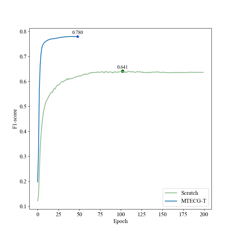
Figure 2: Performance comparison between masked pre-training and training from scratch on the Fuwai dataset. The optimal epoch for masked pre-training is found to be 48, whereas for training from scratch, it is 102.

4.4 Ablation study

In the ablation study, we explore the properties of important components for the proposed method on the Fuwai dataset, and report the marco F1 score on the validation set.

4.4.1 Masking ratio

The validation marco F1 scores of the proposed MTECG-T under multiple masking ratios are summarized in Figure 3 (A). The optimal masking ratio of the proposed method is 25% and it performs stably well across a broad range of ratios (5%-75%). Interestingly, we observed that even at the extreme ratios of 1% and 99%, our proposed method significantly outperforms the model trained from scratch. These findings highlight the effectiveness of the masked pre-training.

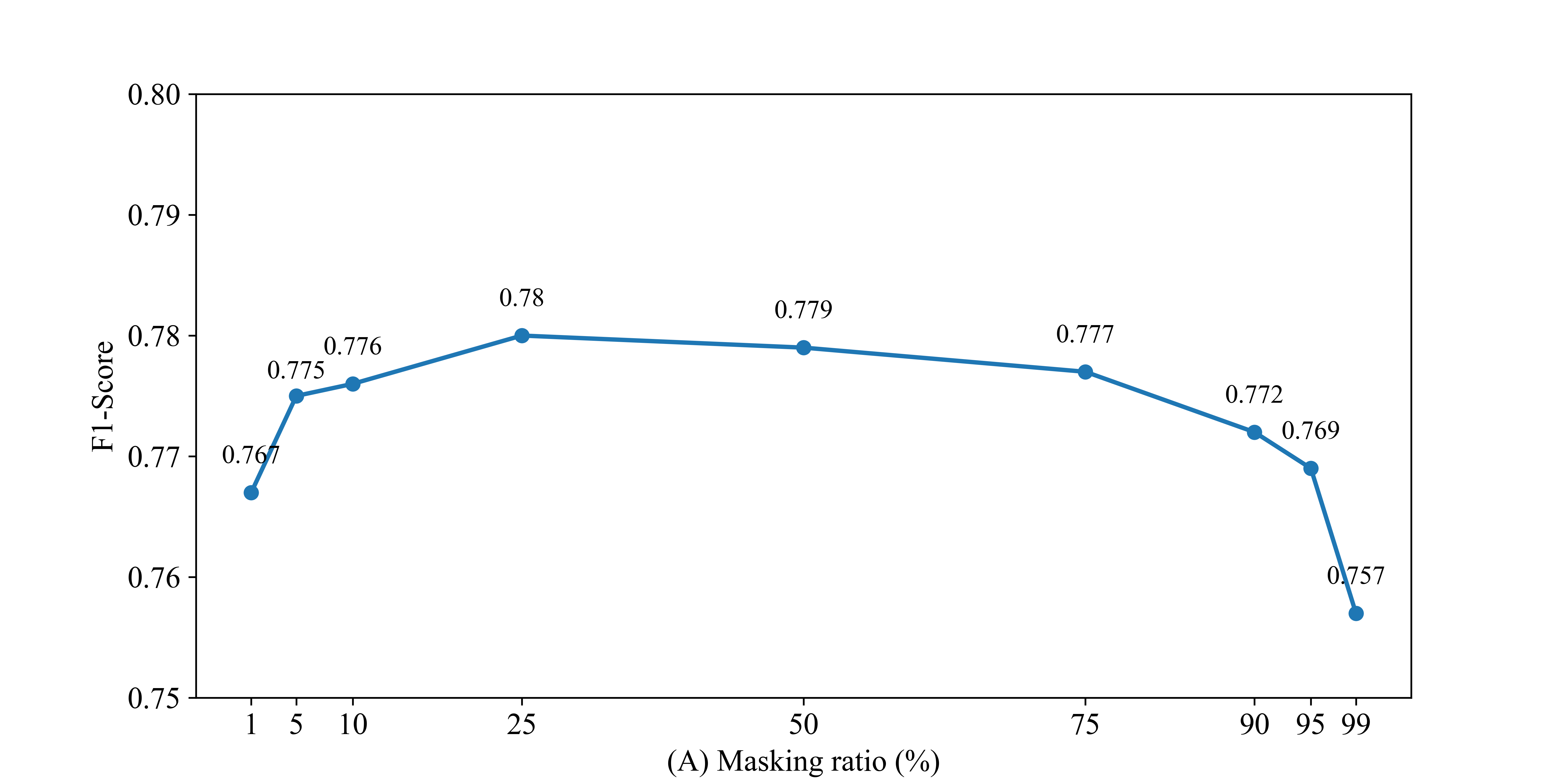
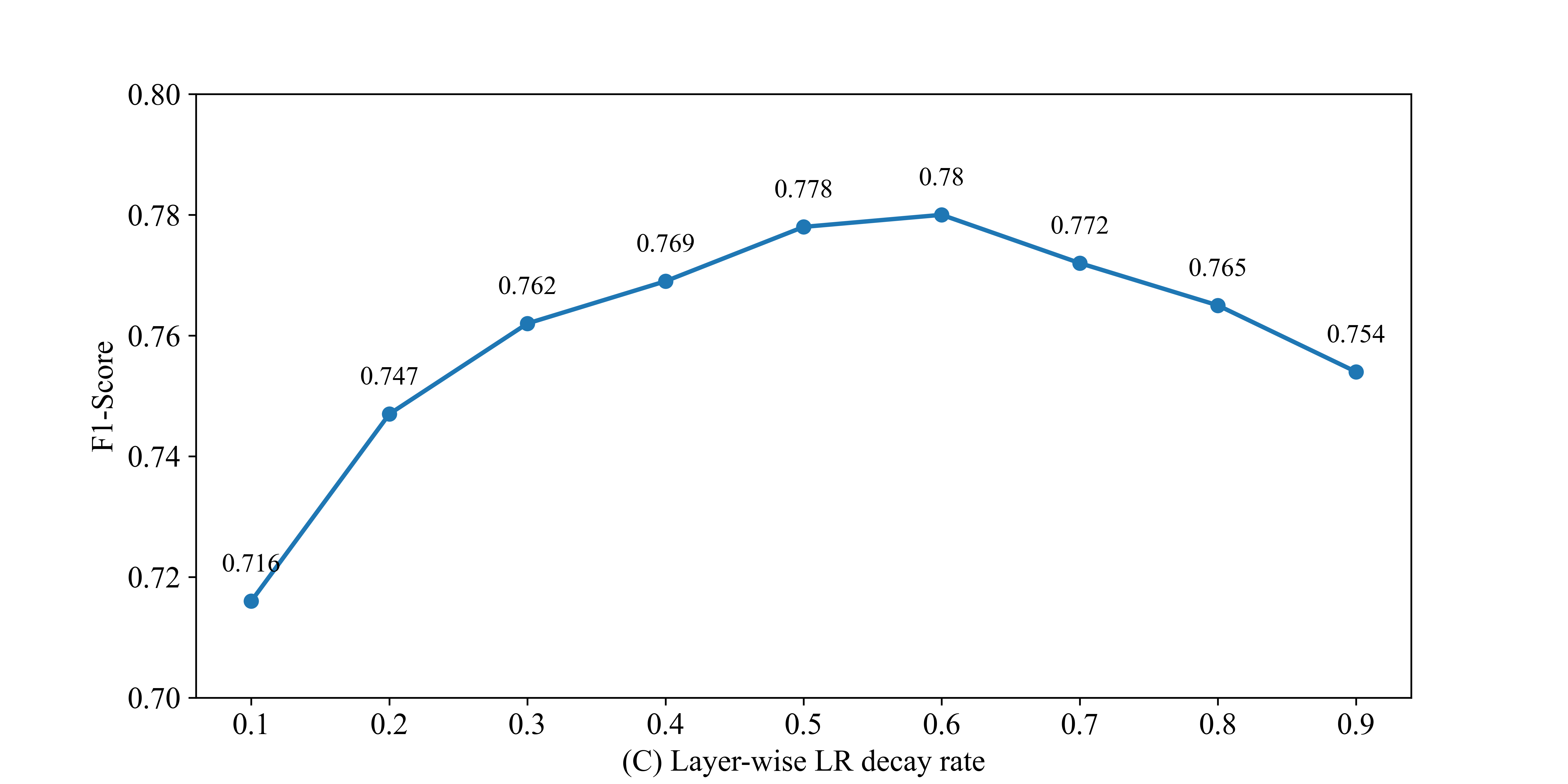
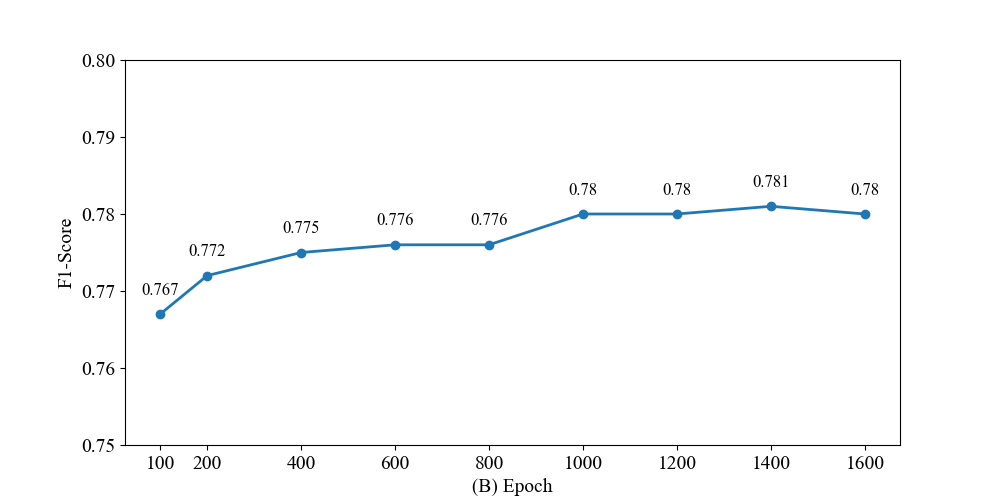
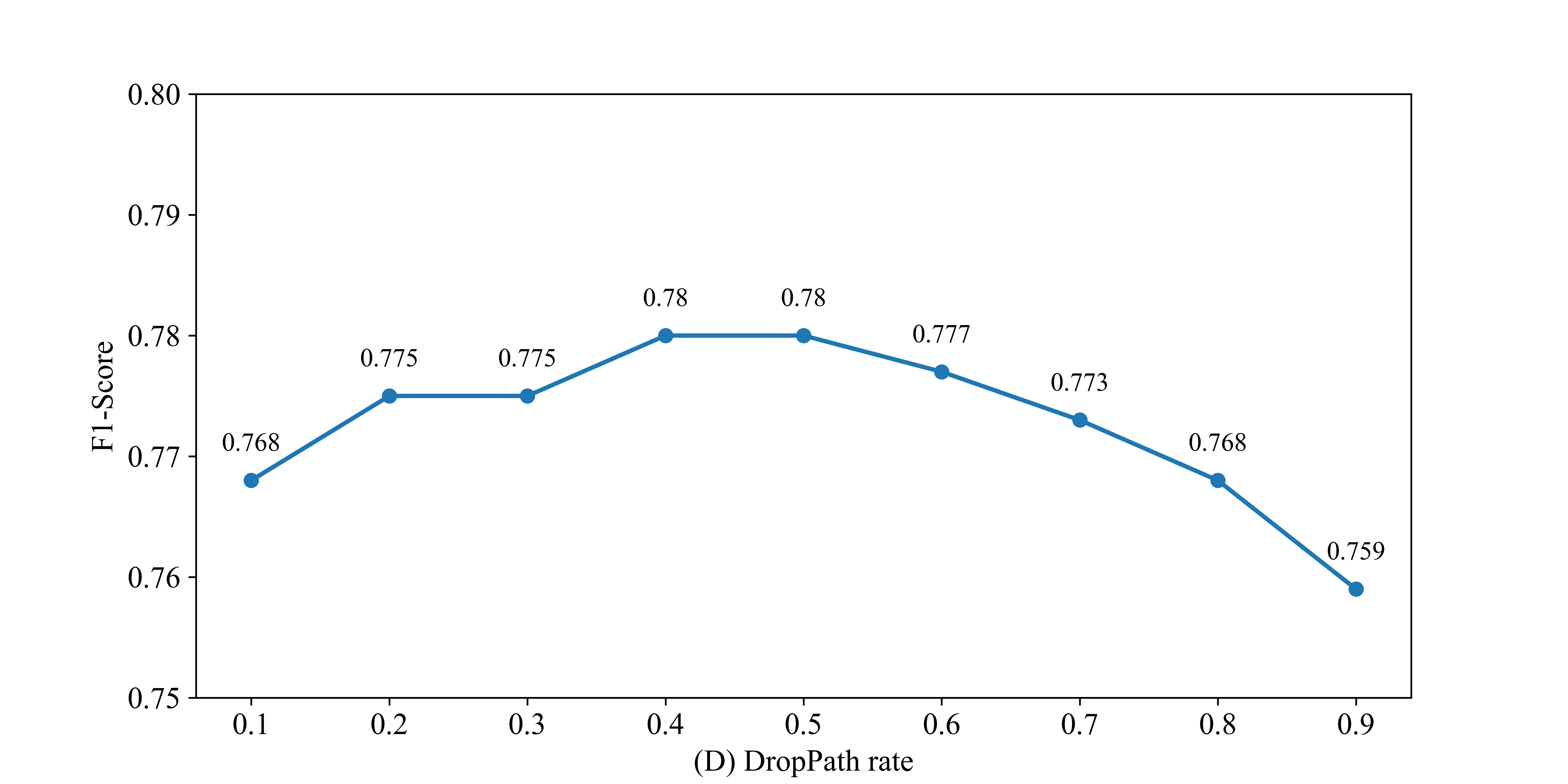
Figure 3: Classification performance in the ablation study. The first column, from top to bottom, corresponds to masking ratio and pre-training schedule lengths, respectively. Similarly, the second column, from top to bottom, corresponds to layer-wise LR decay and DropPath rate, respectively.

4.4.2 Training schedule

We investigate the influence of the pre-training schedule length on the fine-tuning performance. Figure 3 (B) presents our findings. The performance improves with longer training and begins to saturate at 1000 epochs. Interestingly, even with shorter training schedules that had not yet reached saturation, such as the 100-epoch pre-training case, the proposed method exhibits significantly superior performance compared to the model trained from scratch.

4.4.3 Reconstruction target

In this subsection, we compare different reconstruction targets. Figure 4 presents the reconstruction examples from one patient in the validation set and the corresponding fine-tuning performance. Our experimental results clearly demonstrate the beneficial impact of two transformation operations, i.e., per-segment normalization and squaring operation. We observe that both operations fluctuate the original signals, which might enhance the local contrast and amplify subtle changes.

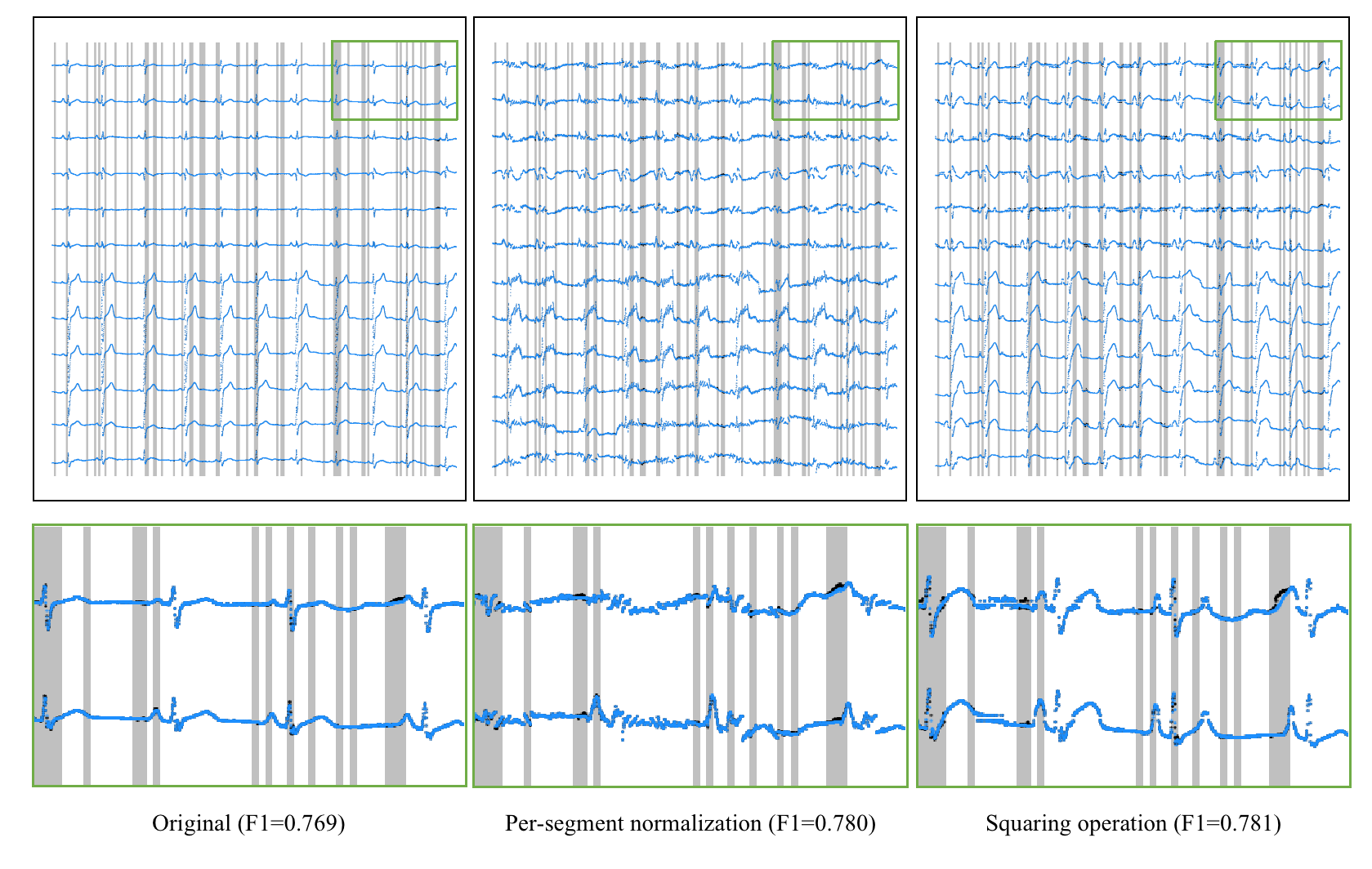
Figure 4: Reconstruction examples from one patient in the validation set under different reconstruction targets. The first row corresponds to the whole ECG signal, while the second row corresponds to a sequence of signal segments. The columns represent the original, per-segment normalization (4), and squaring operation (5) targets, respectively. The gray regions indicate the masked segments. The black point represents the original signal, while the blue point within the masked region represents the reconstructed signal.

4.4.4 Fine-tuning strategy

We investigate the effects of regularization hyper-parameters, layer-wise LR decay (Bao et al., 2021; Clark et al., 2020) and DropPath (Huang et al., 2016) rate on the fine-tuning performance. The results are presented in Figure 3 (C and D), which show the performance across a range of hyper-parameter values from 0.1 to 0.9. The layer-wise LR decay rate of 0.6 is identified as the optimal setting, while for the DropPath rate, options of 0.4 and 0.5 are considered. However, for simplicity, a DropPath rate of 0.4 is utilized later on. Interestingly, we observe that the performance is slightly more sensitive to these hyper-parameters than to the masking ratio.

Furthermore, we conducted experiments on the encoded auxiliary token and segments for classification and found that their performances are comparable. Specifically, when using all encoded segments for classification through global pooling, the macro validation F1 score is 0.780, while using the auxiliary token directly yields a macro F1 score of 0.779.

4.5 Scaling experiments

Noting that the model capacity matters to the generalization ability and the clinical application, we adopt Transformer of different model size for experiments, including MTECG-A (Atomic), MTECG-M (Molecular), MTECG-T(Tiny), MTECG-S (Small) and MTECG-B (Base), for which we change the number of heads $h$ for the encoder, keeping $D/h=64$ and the layers $L=12$. Table 1 summarizes the architectures and their fine-tuning performance in the experiments. The fine-tuning performance initially increase and then fall as the model size increases.

Table 1: Variants of our MTECG architecture and their fine-tuning performance. The #params column represents the number of trainable parameters.

Model Segment size $D$ $h$ $L$ #params F1 MTECG-A 25 64 1 12 0.9M 0.752 MTECG-M 25 128 2 12 2.7 M 0.775 MTECG-T 25 192 3 12 5.7 M 0.780 MTECG-S 25 384 6 12 21. 8M 0.775 MTECG-B 25 768 12 12 85.8M 0.776

4.6 Comparison with the state-of-the-art algorithms

We compare our proposed MTECG-T with three state-of-the-art approaches. Those are (i) CLECG(Chen et al., 2021), (ii) MaeFE (Zhang et al., 2022), and (iii) BaT (Li et al., 2021). These methods represent distinct techniques in the domain of ECG classification, with CLECG utilizing contrastive learning, MaeFE employing masked modeling, and BaT leveraging a Transformer-based model. MTECG-T, CLECG and MaeFE follows the pretraining-finetuning paradigm, while BaT can be trained from scratch. For CLECG, we adopt xresnet1d101 (Strodthoff et al., 2020) as the backbone. For MaeFE, we use MTAE masking strategy and the suggested ViT backbone (Zhang et al., 2022).

We conduct experiments using 3 settings, denoted by Fuwai, PTB-XL and PCinC in Table 2. For the two stage methods, including MTECG-T, CLECG and MaeFE, we develop the algorithm as follow. In the first setting, we pre-train and fine-tune on the training set of Fuwai dataset. In the second setting, we pre-train on the PCinC dataset excluding PTB-XL and then fine-tune on the training set of PTB-XL. In the third setting, we pre-train and fine-tune on the training set of PCinC dataset. For the one stage method, i.e., BaT, we train the model from scratch on Fuwai, PTB-XL and PCinC separately. We adopt the hyper-parameters suggested in the reference papers (Chen et al., 2021; Zhang et al., 2022; Li et al., 2021; Strodthoff et al., 2020) . Particularly, the training epochs of MaeFE in pre-training and fine-tuning are 9000 and 2000, respectively, both of which are much larger than that of the proposed method. The algorithm comparison is demonstrated in Table 2, from which we can see MTECG-T significantly outperforms the alternatives across all datasets.

Table 2: Prediction performance on 3 real datasets. Reported are the macro F1 scores on the testing set of each dataset.

Datasets CLECG MaeFE BaT MTECG-T (Chen et al., 2021) (Zhang et al., 2022) (Li et al., 2021) Fuwai 0.740 0.705 0.702 0.765 PTB-XL 0.518 0.533 0.462 0.586 PCinC 0.590 0.605 0.561 0.662

5 Discussion

The application of deep learning for ECG classification has gained significant popularity in the domains of medicine and computer science. In this study, we extensively evaluate and explore the application of the innovative Transformer architecture and masked modeling methods, leveraging both private and publicly available ECG datasets. Our experiments demonstrate promising performance of the proposed methods, which also underscore their potential effectiveness in clinical applications. Moreover, our findings raise several questions as follows.

1. A standard ECG is worth 200 words? In this paper, the segments, architectures and training strategies are similar to techniques used in NLP. One may wonder whether the deep learning methods for ECG will also follow a similar trajectory as NLP. It is important to acknowledge that the simple self-supervised learning method in NLP enables benefits through model scaling. However, our scaling experiments demonstrate that the masked pre-training method fails to sustain scalable benefits, with performance exhibiting an initial rise followed by a subsequent decline as the model size increases. One potential explanation could be the insufficient size of the training data. Although larger than almost all publicly available ECG datasets, our dataset is still relatively small compared to the datasets commonly used in NLP and CV pre-training tasks.

2. The Transformer is suitable for ECG time series in lightweight regimes? On the other hand, our experiments show that lightweight Transformers could achieve excellent performance in ECG classification if proper training strategies are adopted. Note that our networks stem from the vanilla ViT. The findings break the popular conception that vanilla Transformers are not suitable for classification tasks in lightweight regimes, which is consistent with the observation of Wang et al. (2023a). These facts also suggest that employing appropriate pre-training techniques the naive network architectures could be better than specifically designed ones. It is worth to mention the naive lightweight model are friendly to deployment in the clinical environment.

3. How important the training recipe is in the masked modeling? Previous emphasis was primarily on the masking strategy, training schedule length, and reconstruction target. However, in this work, we demonstrate that the fine-tuning performance is not only sensitive to the those components, but also to other components such as the layer-wise LR decay and DropPath rate. These findings indicate that the successful application of masked modeling in domain-specific tasks might rely on the implementation of proper pre-training and fine-tuning recipes.

4. Transformers or CNNs for ECG classification? Transformers have shown remarkable performance in various visual benchmarks, often matching or surpassing that of CNNs. One may curious about whether Transformers could potentially replace CNNs for ECG classification tasks. We compare the Transformer-based model with masked pre-training (MTECG-T) with the benchmark CNN-based model with contrastive pre-training (CLECG), and observe that the Transformer-based model achieve significantly better performance. However, we cannot conclude that Transformer is a better architecture than CNN for ECG classification due to the different pre-training strategy. It would be interesting to investigate whether CNNs could achieve a comparable performance by developing an appropriate masked pre-training method.

5. Can the proposed method be utilized in novel clinical scenarios? In recent years, the field of ECG has experienced remarkable advancements, particularly in the area of deep learning. Numerous studies have revealed the ability of deep learning models to identify subtle changes in ECG signals that are unrecognizable by the human eye (Siontis et al., 2021). Remarkably, these subtle patterns may be indicative of asymptomatic diseases, such as asymptomatic left ventricular systolic dysfunction (Attia et al., 2019, 2022; Yao et al., 2021). The detection of these patterns introduces novel clinical scenarios for ECG analysis (Somani et al., 2021), where the labels for ECG are obtained from alternative modalities such as echocardiogram and computed tomography. However, a significant challenge lies in the large number of ECG signals that lack corresponding labels from other modalities. Previous research has typically excluded these unlabeled ECG records (Siontis et al., 2021; Somani et al., 2021). Our proposed method, characterized by its self-supervised nature, could effectively utilize these unlabeled ECG records. Consequently, it becomes intriguing to explore the performance of the proposed method in such scenarios.

6 Conclusion

In conclusion, the paper presents a useful masked Transformer method which expands the application of MAE to time-series ECG data. A comprehensive ECG dataset, annotated by medical experts, is constructed to optimize training strategies for the proposed method. The experiments show that even the naive Transformer architecture can achieves remarkable results in ECG classification when proper training strategies are adopted. The results verify the effectiveness of masked modeling and highlight the importance of factors including fluctuated reconstruction targets, training schedule length, layer-wise LR decay, and DropPath rate. In addition, the experiments on both private and public datasets confirm the merits of the proposed MTECG-T, which primary stems from vanilla ViT and offers deployment-friendly features. These facts underscore the promising potential of our approach for ECG classification and its applicability in the clinical environment.

References

- Attia et al. (2022) Attia, Z. I., Harmon, D. M., Dugan, J., Manka, L., Lopez-Jimenez, F., Lerman, A., Siontis, K. C., Noseworthy, P. A., Yao, X., Klavetter, E. W. et al. (2022) Prospective evaluation of smartwatch-enabled detection of left ventricular dysfunction. Nature Medicine, 1–7.
- Attia et al. (2019) Attia, Z. I., Kapa, S., Lopez-Jimenez, F., McKie, P. M., Ladewig, D. J., Satam, G., Pellikka, P. A., Enriquez-Sarano, M., Noseworthy, P. A., Munger, T. M. et al. (2019) Screening for cardiac contractile dysfunction using an artificial intelligence–enabled electrocardiogram. Nature Medicine, 25, 70–74.
- Ba et al. (2016) Ba, J. L., Kiros, J. R. and Hinton, G. E. (2016) Layer normalization. arXiv preprint arXiv:1607.06450.
- Bagui and Li (2021) Bagui, S. and Li, K. (2021) Resampling imbalanced data for network intrusion detection datasets. Journal of Big Data, 8, 1–41.
- Bao et al. (2021) Bao, H., Dong, L., Piao, S. and Wei, F. (2021) Beit: Bert pre-training of image transformers. arXiv preprint arXiv:2106.08254.
- Bousseljot et al. (1995) Bousseljot, R., Kreiseler, D. and Schnabel, A. (1995) Nutzung der ekg-signaldatenbank cardiodat der ptb über das internet.
- Chen et al. (2021) Chen, H., Wang, G., Zhang, G., Zhang, P. and Yang, H. (2021) Clecg: A novel contrastive learning framework for electrocardiogram arrhythmia classification. IEEE Signal Processing Letters, 28, 1993–1997.
- Clark et al. (2020) Clark, K., Luong, M.-T., Le, Q. V. and Manning, C. D. (2020) Electra: Pre-training text encoders as discriminators rather than generators. arXiv preprint arXiv:2003.10555.
- Deng et al. (2009) Deng, J., Dong, W., Socher, R., Li, L.-J., Li, K. and Fei-Fei, L. (2009) Imagenet: A large-scale hierarchical image database. In 2009 IEEE Conference on Computer Vision and Pattern Recognition, 248–255. IEEE.
- Devlin et al. (2019) Devlin, J., Chang, M.-W., Lee, K. and Toutanova, K. (2019) Bert: Pre-training of deep bidirectional transformers for language understanding. NAACL.
- Dosovitskiy et al. (2020) Dosovitskiy, A., Beyer, L., Kolesnikov, A., Weissenborn, D., Zhai, X., Unterthiner, T., Dehghani, M., Minderer, M., Heigold, G., Gelly, S. et al. (2020) An image is worth 16x16 words: Transformers for image recognition at scale. arXiv preprint arXiv:2010.11929.
- Gutmann and Hyvärinen (2010) Gutmann, M. and Hyvärinen, A. (2010) Noise-contrastive estimation: A new estimation principle for unnormalized statistical models. In Proceedings of the thirteenth international conference on artificial intelligence and statistics, 297–304. JMLR Workshop and Conference Proceedings.
- Han et al. (2022) Han, K., Wang, Y., Chen, H., Chen, X., Guo, J., Liu, Z., Tang, Y., Xiao, A., Xu, C., Xu, Y. et al. (2022) A survey on vision transformer. IEEE Transactions on Pattern Analysis and Machine Intelligence, 45, 87–110.
- Hannun et al. (2019) Hannun, A. Y., Rajpurkar, P., Haghpanahi, M., Tison, G. H., Bourn, C., Turakhia, M. P. and Ng, A. Y. (2019) Cardiologist-level arrhythmia detection and classification in ambulatory electrocardiograms using a deep neural network. Nature Medicine, 25, 65–69.
- He et al. (2022) He, K., Chen, X., Xie, S., Li, Y., Dollár, P. and Girshick, R. (2022) Masked autoencoders are scalable vision learners. In Proceedings of the IEEE/CVF Conference on Computer Vision and Pattern Recognition, 16000–16009.
- Hong et al. (2020) Hong, S., Zhou, Y., Shang, J., Xiao, C. and Sun, J. (2020) Opportunities and challenges of deep learning methods for electrocardiogram data: A systematic review. Computers in Biology and Medicine, 122, 103801.
- Huang et al. (2016) Huang, G., Sun, Y., Liu, Z., Sedra, D. and Weinberger, K. Q. (2016) Deep networks with stochastic depth. In Computer Vision–ECCV 2016: 14th European Conference, Amsterdam, The Netherlands, October 11–14, 2016, Proceedings, Part IV 14, 646–661. Springer.
- Hughes et al. (2021) Hughes, J. W., Olgin, J. E., Avram, R., Abreau, S. A., Sittler, T., Radia, K., Hsia, H., Walters, T., Lee, B., Gonzalez, J. E. et al. (2021) Performance of a convolutional neural network and explainability technique for 12-lead electrocardiogram interpretation. JAMA Cardiology, 6, 1285–1295.
- Khan et al. (2022) Khan, S., Naseer, M., Hayat, M., Zamir, S. W., Khan, F. S. and Shah, M. (2022) Transformers in vision: A survey. ACM Computing Surveys (CSUR), 54, 1–41.
- Kiyasseh et al. (2021) Kiyasseh, D., Zhu, T. and Clifton, D. A. (2021) Clocs: Contrastive learning of cardiac signals across space, time, and patients. In International Conference on Machine Learning, 5606–5615. PMLR.
- Ko et al. (2020) Ko, W.-Y., Siontis, K. C., Attia, Z. I., Carter, R. E., Kapa, S., Ommen, S. R., Demuth, S. J., Ackerman, M. J., Gersh, B. J., Arruda-Olson, A. M. et al. (2020) Detection of hypertrophic cardiomyopathy using a convolutional neural network-enabled electrocardiogram. Journal of the American College of Cardiology, 75, 722–733.
- Krishnan et al. (2022) Krishnan, R., Rajpurkar, P. and Topol, E. J. (2022) Self-supervised learning in medicine and healthcare. Nature Biomedical Engineering, 1–7.
- Li et al. (2021) Li, X., Li, C., Wei, Y., Sun, Y., Wei, J., Li, X. and Qian, B. (2021) Bat: Beat-aligned transformer for electrocardiogram classification. In 2021 IEEE International Conference on Data Mining (ICDM), 320–329. IEEE.
- Liu et al. (2018) Liu, F., Liu, C., Zhao, L., Zhang, X., Wu, X., Xu, X., Liu, Y., Ma, C., Wei, S., He, Z. et al. (2018) An open access database for evaluating the algorithms of electrocardiogram rhythm and morphology abnormality detection. Journal of Medical Imaging and Health Informatics, 8, 1368–1373.
- Liu et al. (2021) Liu, X., Zhang, F., Hou, Z., Mian, L., Wang, Z., Zhang, J. and Tang, J. (2021) Self-supervised learning: Generative or contrastive. IEEE Transactions on Knowledge and Data Engineering, 35, 857–876.
- Mehari and Strodthoff (2022) Mehari, T. and Strodthoff, N. (2022) Self-supervised representation learning from 12-lead ecg data. Computers in Biology and Medicine, 141, 105114.
- Naseer et al. (2021) Naseer, M. M., Ranasinghe, K., Khan, S. H., Hayat, M., Shahbaz Khan, F. and Yang, M.-H. (2021) Intriguing properties of vision transformers. Advances in Neural Information Processing Systems, 34, 23296–23308.
- Oh et al. (2022) Oh, J., Chung, H., Kwon, J.-m., Hong, D.-g. and Choi, E. (2022) Lead-agnostic self-supervised learning for local and global representations of electrocardiogram. In Conference on Health, Inference, and Learning, 338–353. PMLR.
- Pyakillya et al. (2017) Pyakillya, B., Kazachenko, N. and Mikhailovsky, N. (2017) Deep learning for ecg classification. In Journal of physics: conference series, vol. 913, 012004. IOP Publishing.
- Radford et al. (2018) Radford, A., Narasimhan, K., Salimans, T., Sutskever, I. et al. (2018) Improving language understanding by generative pre-training.
- Reyna et al. (2021) Reyna, M. A., Sadr, N., Alday, E. A. P., Gu, A., Shah, A. J., Robichaux, C., Rad, A. B., Elola, A., Seyedi, S., Ansari, S. et al. (2021) Will two do? varying dimensions in electrocardiography: the physionet/computing in cardiology challenge 2021. In 2021 Computing in Cardiology (CinC), vol. 48, 1–4. IEEE.
- Reyna et al. (2022) — (2022) Issues in the automated classification of multilead ecgs using heterogeneous labels and populations. Physiological Measurement, 43, 084001.
- Ribeiro et al. (2020) Ribeiro, A. H., Ribeiro, M. H., Paixão, G. M., Oliveira, D. M., Gomes, P. R., Canazart, J. A., Ferreira, M. P., Andersson, C. R., Macfarlane, P. W., Meira Jr, W. et al. (2020) Automatic diagnosis of the 12-lead ecg using a deep neural network. Nature Communications, 11, 1760.
- Sharma and Sunkaria (2021) Sharma, L. D. and Sunkaria, R. K. (2021) Detection and delineation of the enigmatic u-wave in an electrocardiogram. International Journal of Information Technology, 13, 2525–2532.
- Siontis et al. (2021) Siontis, K. C., Noseworthy, P. A., Attia, Z. I. and Friedman, P. A. (2021) Artificial intelligence-enhanced electrocardiography in cardiovascular disease management. Nature Reviews Cardiology, 18, 465–478.
- Somani et al. (2021) Somani, S., Russak, A. J., Richter, F., Zhao, S., Vaid, A., Chaudhry, F., De Freitas, J. K., Naik, N., Miotto, R., Nadkarni, G. N. et al. (2021) Deep learning and the electrocardiogram: review of the current state-of-the-art. EP Europace, 23, 1179–1191.
- Strodthoff et al. (2023) Strodthoff, N., Mehari, T., Nagel, C., Aston, P. J., Sundar, A., Graff, C., Kanters, J. K., Haverkamp, W., Dössel, O., Loewe, A. et al. (2023) Ptb-xl+, a comprehensive electrocardiographic feature dataset. Scientific Data, 10, 279.
- Strodthoff et al. (2020) Strodthoff, N., Wagner, P., Schaeffter, T. and Samek, W. (2020) Deep learning for ecg analysis: Benchmarks and insights from ptb-xl. IEEE Journal of Biomedical and Health Informatics, 25, 1519–1528.
- Tihonenko et al. (2007) Tihonenko, V., Khaustov, A., Ivanov, S., Rivin, A. et al. (2007) St.-petersburg institute of cardiological technics 12-lead arrhythmia database. Dataset on Physionet. org.
- Vaswani et al. (2017) Vaswani, A., Shazeer, N., Parmar, N., Uszkoreit, J., Jones, L., Gomez, A. N., Kaiser, Ł. and Polosukhin, I. (2017) Attention is all you need. Advances in Neural Information Processing Systems, 30.
- Wagner et al. (2020) Wagner, P., Strodthoff, N., Bousseljot, R.-D., Kreiseler, D., Lunze, F. I., Samek, W. and Schaeffter, T. (2020) Ptb-xl, a large publicly available electrocardiography dataset. Scientific Data, 7, 1–15.
- Wang et al. (2023a) Wang, S., Gao, J., Li, Z., Zhang, X. and Hu, W. (2023a) A closer look at self-supervised lightweight vision transformers. In International Conference on Machine Learning, 35624–35641. PMLR.
- Wang et al. (2023b) Wang, Z., Wang, Y., Hu, H. and Li, P. (2023b) Contrastive learning with consistent representations. arXiv preprint arXiv:2302.01541.
- Wei et al. (2019) Wei, Y., Wang, X., Guan, W., Nie, L., Lin, Z. and Chen, B. (2019) Neural multimodal cooperative learning toward micro-video understanding. IEEE Transactions on Image Processing, 29, 1–14.
- Wen et al. (2022) Wen, Q., Zhou, T., Zhang, C., Chen, W., Ma, Z., Yan, J. and Sun, L. (2022) Transformers in time series: A survey. arXiv preprint arXiv:2202.07125.
- Xie et al. (2022) Xie, Z., Zhang, Z., Cao, Y., Lin, Y., Bao, J., Yao, Z., Dai, Q. and Hu, H. (2022) Simmim: A simple framework for masked image modeling. In Proceedings of the IEEE/CVF Conference on Computer Vision and Pattern Recognition, 9653–9663.
- Yao et al. (2021) Yao, X., Rushlow, D. R., Inselman, J. W., McCoy, R. G., Thacher, T. D., Behnken, E. M., Bernard, M. E., Rosas, S. L., Akfaly, A., Misra, A. et al. (2021) Artificial intelligence–enabled electrocardiograms for identification of patients with low ejection fraction: a pragmatic, randomized clinical trial. Nature Medicine, 27, 815–819.
- Zhang et al. (2022) Zhang, H., Liu, W., Shi, J., Chang, S., Wang, H., He, J. and Huang, Q. (2022) Maefe: Masked autoencoders family of electrocardiogram for self-supervised pretraining and transfer learning. IEEE Transactions on Instrumentation and Measurement, 72, 1–15.
- Zheng et al. (2020a) Zheng, J., Chu, H., Struppa, D., Zhang, J., Yacoub, S. M., El-Askary, H., Chang, A., Ehwerhemuepha, L., Abudayyeh, I., Barrett, A. et al. (2020a) Optimal multi-stage arrhythmia classification approach. Scientific Reports, 10, 1–17.
- Zheng et al. (2020b) Zheng, J., Zhang, J., Danioko, S., Yao, H., Guo, H. and Rakovski, C. (2020b) A 12-lead electrocardiogram database for arrhythmia research covering more than 10,000 patients. Scientific Data, 7, 1–8.